Replica Symmetry Breaking for the Integrable Two-Site Sachdev-Ye-Kitaev Model

Abstract

We analyze a two-body nonhermitian two-site Sachdev-Ye-Kitaev model with the couplings of one site complex conjugated to the other site. This model, with no explicit coupling between the sites, shows an infinite number of second order phase transitions which is a consequence of the factorization of the partition function into a product over Matsubara frequencies. We calculate the quenched free energy in two different ways, first in terms of the single-particle energies, and second by solving the Schwinger-Dyson equations of the two-site model. The first calculation can be done entirely in terms of a one-site model. The conjugate replica enters due to non-analyticities when Matsubara frequencies enter the spectral support of the coupling matrix. The second calculation is based on the replica trick of the two-site partition function. Both methods give the same result. The free-fermion partition function can also be rephrased as a matrix model for the coupling matrix. Up to minor details, this model is the random matrix model that describes the chiral phase transition of QCD, and the order parameter of the two-body model corresponds to the chiral condensate of QCD. Comparing to the corresponding four-body model, we are able to determine which features of the free energy are due to chaotic nature of the four-body model. The high-temperature phase of both models is entropy dominated, and in both cases the free energy is determined by the spectral density. The chaotic four-body SYK model has a low-temperature phase whose free energy is almost temperature-independent, signaling an effective gap of the theory even though the actual spectrum does not exhibit a gap. On the other hand the low-temperature free energy of the two-body SYK model is not flat, in fact it oscillates to arbitrarily low temperature. This indicates a less desirable feature that the entropy of the two-body model is not always positive in the low-temperature phase, which most likely is a consequence of the nonhermiticity.

I Introduction

In 1971 George Uhlenbeck asked Freeman Dyson “Which nucleus has levels distributed according to the semi-circle law?” dyson1996selected . As answer to his criticism, Dyson published his last paper on Random Matrix Theory Dyson:1972tm in which he introduced a Brownian motion process to construct an ensemble of random matrices with an arbitrary level density, in particular the nuclear level density given by the Bethe formula bethe1936 ,

$$\rho(E)=be^{c\sqrt{E}}.$$ (1)

Uhlenbeck could have asked a different question, namely “Is the nuclear force an all–to–all many-body interaction?” which is the case for the Wigner-Dyson ensembles. This question led French, Wong, Bohigas, Flores and Mon french1970 ; french1971 ; bohigas1971 ; bohigas1971a ; mon1975 around the same time to the introduction of the two-body (which in the SYK literature is known as a four-body interaction) random ensemble which reflects the two-body nature of the nuclear interaction. It took until 2015, through the seminal work of Kitaev kitaev2015 ; maldacena2016 , to realize that Uhlenbeck’s criticism could also have been addressed by this work. The two-body random ensemble, in particular the version of the model introduced by Mon and French mon1975 , is now known as the complex Sachdev-Ye-Kitaev (SYK) model sachdev1993 ; sachdev2015 .

Since the pioneering work of Wigner, Dyson, Gaudin and Mehta wigner1951 ; mehta1960density ; dyson1962statistical ; dyson1962statisticalII ; dyson1962statisticalIII ; dyson1963statisticalI ; mehta1963statisticalII ; dyson1962threefold ; Dyson:1972tm random matrix theory has been applied to virtually all areas of physics and even outside of physics, see the comprehensive review by Guhr, Müller Groeling and Weidenmüller guhr1998 . In this paper we study nonhermitian random matrix theories which were first introduced by Ginibre ginibre1965 , but have also been applied to many areas of physics. For example, the distribution of poles of S-matrices Verbaarschot1984a ; Verbaarschot:1985jn ; sommers1999s , the Hatano-Nelson model hatano1996localization ; efetov1997directed ; brouwer1998delocalization , dissipative quantum systems fyodorov1997 ; akemann2019universal ; li2021spectral ; sa2021lindbladian , QCD at nonzero chemical potential stephanov1996 ; Janik:1996va ; Verbaarschot:2000dy ; Osborn:2004rf ; Akemann:2004dr ; Osborn:2005ss ; Kanazawa:2009en ; kanazawa2021new ; kanazawa2021complex and PT-symmetric systems bender1998 , to mention a few. Nonhermitian random matrices were classified halasz:1997fc ; bernard2002classification ; Magnea:2007yk ; kawabata2019symmetry ; Garcia-Garcia:2021rle along the lines of the classification of Hermitian random matrices dyson1962threefold ; Dyson:1972tm ; Verbaarschot:1994qf ; Altland:1997zz . A recent review of nonhermitian physics was given by Ashida, Gong and Ueda ashida2020non .

The possibility of a nonhermitian version of the Sachdev-Ye-Kitaev (SYK) model was originally suggested by Maldacena and Qi maldacena2018 ; Garcia-Garcia:2019poj as a two-site SYK model for Euclidean wormholes without explicit coupling between the two SYK models (the only coupling is through the randomness) and was studied in detail in subsequent papers Garcia-Garcia:2020ttf ; Garcia-Garcia:2021elz ; Garcia-Garcia:2021rle ; Garcia-Garcia:2022 . In this model, the Left (L) and Right (R) partition functions are complex conjugate to each other, and each of them has $N/2$ Majorana fermions so that energy levels of the $q$-body Hamiltonian

$$H=H_{L}\otimes\mathbb{1}+\mathbb{1}\otimes H_{R},$$ (2)

are given $\{E_{k}+E_{l}^{*}\}$ if the $\{E_{k}\}$ are the eigenvalues of $H_{L}$. Therefore the partition function factorizes as

$$Z=Z_{L}Z_{R}=Z_{L}Z_{L}^{*}$$ (3)

and is necessarily positive definite.

One of the main conclusions from these studies is that the chaotic model has a first order phase transition which separates the low-temperature phase from the high-temperature phase. In the high-temperature phase, the average of the partition function factorizes

$$\langle Z\rangle=\langle Z_{L}\rangle\langle Z_{L}^{*}\rangle$$ (4)

and the free energy follows from the eigenvalue density of the one-site Hamiltonian. Because of the complex phases of the eigenvalues the average partition function is exponentially suppressed due to cancellations. In the case of maximum nonhermiticity, when the eigenvalue density is isotropic in the complex plane, the partition function $\langle Z_{L}\rangle$ becomes temperature independent and the free energy is determined by the total number of states $F=-T\frac{N}{2}\log 2$. It is clear that this result cannot be correct at low temperature when $F\to-|E_{0}|$ with $E_{0}$ the ground state energy. The only possibility is that the low-temperature phase receives contributions from the correlations of the eigenvalues of the $L$ and $R$ Hamiltonians. Indeed, for the $q=4$ SYK model the free energy in the low-temperature phase is entirely determined by the two-point correlations of the eigenvalues Garcia-Garcia:2021elz ; Garcia-Garcia:2022 . The reason that this can happen is the exponential suppression of the single site partition function due to the complex phase of the eigenvalues. The dynamics of the $q=4$ SYK model is chaotic with eigenvalue correlations in the universality class of the Ginibre model. The universal two-point correlations give rise to a temperature-independent free energy at low temperatures. This also explains that results obtained by solving the Schwinger-Dyson equations are very close to the results for the Ginibre random matrix ensemble. We conclude that the quantum chaotic nature of the model is responsible for a nearly temperature-independent free energy in the low-temperature phase when an actual spectral gap is absent. As a consequence, the free energy of the low-temperature phase of the $q=2$ SYK model, which is integrable and has no spectral gap, has to be different. The goal of this paper is to solve the $q=2$ nonhermitian SYK model to study the effects of chaos and integrability on the phase diagram.

As was the case for the $q=4$ SYK model Garcia-Garcia:2021elz ; Garcia-Garcia:2022 , in this paper we evaluate the quenched free energy in two structurally different ways. First, from the eigenvalues of the SYK Hamiltonian giving the quenched free energy, and second, from the solution of the Schwinger-Dyson equations dyson1949s ; schwinger1951green of the SYK model in $\Sigma G$ formulation, giving the annealed free energy of the two-site SYK model. For $q=2$ it is possible to perform the spectral calculation both analytically and numerically, while for $q=4$ this could only be done numerically by an explicit diagonalization of the SYK Hamiltonian. Also the Schwinger-Dyson equation can be solved analytically for $q=2$ Maldacena:2015waa ; Cotler:2016fpe while for $q=4$ we had to rely on numerical techniques.

The $\Sigma G$ formulation of the SYK model is based on the replica trick for the quenched free energy edwards1971statistical

$$\log Z=\lim_{n\to 0}\frac{Z^{n}-1}{n},$$ (5)

which is known to fail sherrington1972 ; verbaarschot1985 ; zirnbauer1999critique in particular for nonhermitian theories Barbour:1986jf . However, by now it has been well understood how to refine the replica method so that its results can be trusted parisi1979 ; girko2012theory ; stephanov1996 ; mezard1999 ; nishigaki2002a ; kanzieper2002 ; splittorff:2003cu ; sedrakyan2005toda . For Hermitian models the naive replica trick usually gives the correct result for a mean field analysis. This is also the case for the $\Sigma G$ formulation of the SYK model arefeva2018 ; wang2018 . However, as should be clear from the arguments given above, the naive application of the replica trick to the one-site nonhermitian SYK model gives an incorrect result for the quenched free energy of the low-temperature phase. Instead, the quenched free energy of the one-site Hamiltonian is given by the replica limit of the product of the partition function and its complex conjugate. In the case of the one-site partition function, the replica symmetry is broken in the sense that the conjugate replica emerges due to quenching and couples to the original replica. The emergence of conjugate replicas for quenched replicas is well-known in nonhermitian RMT girko2012theory ; efetov1997directed ; feinberg1997non and QCD at nonzero chemical potential stephanov1996 ; Janik:1996va ; Janik:1996xm ; splittorff:2003cu .

We start this paper with a short introduction of the SYK model and the replica trick. Since the $q=2$ SYK model is a Fermi liquid, we can calculate the quenched free energy from a free-fermion formulation of the model, see section III. In section IV we calculate annealed free energy for the $\Sigma G$ formulation of the SYK model for one replica and one conjugate replica. The final result is in complete agreement with the result from the free-fermion calculation. The $\Sigma G$ action of the $q=2$ SYK model is quadratic in $G$ so that it can be integrated out exactly. The result resembles a random matrix $\sigma$-model. In section V, we show that this $\sigma$-model can also directly obtained from the free-fermion description of the $q=2$ SYK model. Concluding remarks are made in section VI and some technical details are worked out in two appendices. In Appendix A we show that the occupation number representation also applies to the nonhermitian SYK model, and in Appendix B, we work out the free-fermion calculation for the case the nonhermiticity is not maximal.

II The $q=2$ nonhermitian SYK model

The Hamiltonian of the $q=2$ nonhermitian SYK model is given by

$$H =i\sum_{i<j}^{N/2}\left(J_{ij}+i\,kM_{ij}\right)\psi_{L}^{i}\psi_{L}^{j}-i\sum_{i<j}^{N/2}\left(J_{ij}-i\,kM_{ij}\right)\psi_{R}^{i}\psi_{R}^{j}$$

$$\equiv H_{L}\otimes\mathbb{1}+\mathbb{1}\otimes H_{R},$$ (6)

where $\psi$ are Majorana fermions and $J,M$ are random couplings. A general $q$-body Hamiltonian would have products of $q$ Majorana fermions. The tensor product structure on the second line of equation (II) follows from an explicit Dirac-matrix representation of $\psi$:

$$\begin{split}\psi_{L}^{i}&=\frac{1}{\sqrt{2}}\gamma_{i}\otimes\mathbb{1},\\ \psi_{R}^{i}&=\frac{1}{\sqrt{2}}\gamma_{c}\otimes\gamma_{i},\end{split}$$ (7)

where $\gamma_{i}$ are the Dirac matrices in $N/2$ dimensions and $\gamma_{c}$ is the corresponding chirality matrix (assuming $N/2$ is even). The variances of the couplings are given by

$$\langle J_{ij}^{2}\rangle=\langle M_{ij}^{2}\rangle={v^{2}}/{(N/2)}$$ (8)

where $v$ is a dimensionful parameter that sets the physical scale. In a representation where the left gamma matrices are real and the right gamma matrices are purely imaginary, the Hamiltonian of a single SYK is anti-symmetric under transposition. The eigenvalues, which are representation independent thus occur in pairs $\pm\lambda_{k}$. In this representation we also have that $H_{L}=H_{R}^{*}$ (with the minus sign from the sum included in $H_{R}$). The spectrum of the Hamiltonian (II) is given by $\pm\lambda_{k}\pm\lambda_{l}^{*}$ if the $\lambda_{k}$ are the eigenvalues of $H_{L}$ with a positive real part. The partition function of this Hamiltonian is necessarily positive

$$Z=Z_{L}Z_{R}=|Z_{L}|^{2},$$ (9)

where $Z_{L(R)}$ is the partition function of the $L(R)$ Hamiltonian. The average partition function will be denoted $\langle Z\rangle$ with the appropriate subscripts. Contrary to $q>2$ the SYK Hamiltonian for $q=2$ is a Fermi liquid with single particle energies $\pm\varepsilon_{k}$ given by the eigenvalues of the coupling matrix, which is an anti-symmetric nonhermitian random matrix. Therefore the quenched partition function is given by

$$\langle\log Z\rangle = \left\langle\log\left[\prod_{k}(e^{-\beta\varepsilon_{k}}+e^{\beta\varepsilon_{k}})\prod_{k}(e^{-\beta\varepsilon_{k}^{*}}+e^{\beta\varepsilon_{k}^{*}})\right]\right\rangle$$ (10)

$$= \sum_{k}\left\langle\log(e^{-\beta\varepsilon_{k}}+e^{\beta\varepsilon_{k}})\right\rangle+\sum_{k}\left\langle\log(e^{-\beta\varepsilon_{k}^{*}}+e^{\beta\varepsilon_{k}^{*}})\right\rangle,$$

and

$$\langle\log Z\rangle=\langle\log Z_{L}\rangle+\langle\log Z_{R}\rangle=2\langle\log Z_{L}\rangle.$$ (11)

For the last equality we have used that the average density of the single particle energies satisfies $\langle\rho_{L}^{\rm sp}(z)\rangle=\langle\rho_{R}^{\rm sp}(z^{*})\rangle$. Therefore, the quenched free energy can be obtained from the one-site partition function, which is a direct consequence of the Fermi-liquid nature of the $q=2$ SYK model.

When we evaluate the quenched free energy of the SYK partition function in the $\Sigma G$ formulation, we will employ the replica trick

$$-\beta F=\langle\log Z\rangle=\lim_{n\to 0}\left\langle\frac{Z^{n}-1}{n}\right\rangle.$$ (12)

For large $N$, the partition function can be evaluated by a saddle point approximation. As was argued in Garcia-Garcia:2021elz ; Garcia-Garcia:2022 , since the partition function $Z=Z_{L}Z_{L}^{*}$ is positive definite, the replica trick is expected to give the correct mean field result with unbroken replica symmetry,

$$\langle Z^{n}\rangle=\langle Z\rangle^{n}.$$ (13)

Therefore, the quenched free energy is equal to the annealed free energy

$$\langle\log Z\rangle=\log\langle Z\rangle,$$ (14)

and it can be calculated by evaluating the partition function for one replica of the two-site Hamiltonian, in other words one replica and one conjugate replica in terms of the one-site Hamiltonian. If the (left-right) replica symmetry is broken, we have that

$$\langle(Z_{L}Z^{*}_{L})^{n}\rangle=\langle Z_{L}Z^{*}_{L}\rangle^{n}\neq\langle Z_{L}\rangle^{n}\langle Z^{*}_{L}\rangle^{n}$$ (15)

so that it is not guaranteed that the quenched free energy can be obtained from the one-site annealed free energy. We will see in section IV that is the case for the low-temperature phase of the $\Sigma G$ formulation of the SYK model. In the literature, the coupling between replicas has been related to the formation of wormholes between black holes Saad:2019lba ; Altland:2021rqn .

Before calculating the annealed free energy from the $\Sigma G$ formulation of the SYK model, in the next section, we will evaluate the average partition function, using the properties of the spectra of anti-symmetric nonhermitian random matrices.

III The free energy of the two-site non-hermitian SYK for $q=2$

Results for the $q=4$ nonhermitian SYK model Garcia-Garcia:2021elz ; Garcia-Garcia:2022 suggest that quantum chaotic dynamics is responsible for a replica-symmetry-breaking (RSB) phase at low temperatures with a temperature-independent free energy. Indeed, the free energy of an integrable nonhermitian model of random uncorrelated energies Garcia-Garcia:2022 exhibits a distinct low-temperature phase with a temperature-dependent free energy. However, the random energy model lacks a natural interpretation as a many-body model. In this section, we test this hypothesis by evaluating quenched free energy of the two-site $q=2$ non-Hermitian SYK model which is a Fermi liquid with energies given by sums of single particle energies. Therefore the many-body eigenvalues obey Poisson statistics which is consistent with a vanishing Lyapunov exponent garcia2018chaotic (obtained by calculating the Out of Time Order Correlator). We will calculate the quenched free energy from the single-particle energy density which is constant inside an ellipse in the complex plane. As argued in previous section, the quenched free energy can be obtained from the one-site partition function. In section IV we will see that the same result can be obtained from the SD equation of the two-site model.

After a change of basis (see appendix A for a demonstration), the one-site Hamiltonian can be expressed as a free Fermi liquid with single-particle energies which are the eigenvalues of the antisymmetric coupling matrix . To be concrete, the Hamiltonian $H_{L}$ in (II) becomes

$$H_{L}=\sum_{k=1}^{N/4}\varepsilon_{k}(2\tilde{c}_{k}c_{k}-1),$$ (16)

where $\varepsilon_{k}$ are the eigenvalues of the coupling matrix $i(J_{ij}+ikM_{ij})/2$ with positive real parts and hence the sum runs up to $k=N/4$ instead of $N/2$. Just as in the Hermitian case Cotler:2016fpe , we have

$$[H_{L},\tilde{c}_{k}]=\varepsilon_{k}\tilde{c}_{k},\quad[H_{L},c_{k}]=-\varepsilon_{k}c_{k}.$$ (17)

with

$$\tilde{c}_{k}^{2}=0,\quad,c_{k}^{2}=0,\quad\{c_{k},\tilde{c}_{l}\}=\delta_{kl}.$$ (18)

Hence, we conclude the many-body energies of $H_{L}$ are given by filling $N/4$ free fermions into the single particle states of (16). We note that generally $c_{k}$ is not the Hermitian conjugate of $\tilde{c}_{k}$, and hence the energy eigenstates are not necessarily orthogonal to each other, which is consistent with the nonhermiticity of the Hamiltonian.

In this free-fermion representation, the quenched free energy of the one-site SYK model, which we shall see to be identical to half the two-site model, is simply

$$\begin{split}F_{L}=-T\langle\log Z_{L}\rangle&=-T\left\langle\sum_{k=1}^{N/4}\log\left(e^{-\varepsilon_{k}/T}+e^{\varepsilon_{k}/T}\right)\right\rangle\\ &=-\frac{T}{2}\int d^{2}z\langle\rho(z)\rangle\log\left(2\cosh\frac{z}{T}\right),\end{split}$$ (19)

where $\langle\rho(z)\rangle$ is the averaged spectral density of the coupling matrix $i(J_{ij}+ikM_{ij})/2$. Notice that since $\varepsilon_{k}$ are only half of the levels of $i(J_{ij}+ikM_{ij})/2$ (those with positive real parts), the integral in the second equality should have only covered half of the support of $\rho(z)$. However, since the integrand is invariant under $z\mapsto-z$, we simply integrate over the whole support and compensate it by a pre-factor of $1/2$.

At large $N$, the averaged spectral density $\langle\rho(z)\rangle$ is a constant inside the ellipse fyodorov1997 ; hastings2001 ; hamazaki2020 ; akemann2022spacing

$$\rho(z)=\frac{N/2}{\pi\epsilon_{0}\upsilon_{0}}\theta\left(1-\frac{x^{2}}{\epsilon_{0}^{2}}-\frac{y^{2}}{\upsilon_{0}^{2}}\right),$$ (20)

where

$$\epsilon_{0}=\frac{1}{\sqrt{1+k^{2}}}v,\quad\upsilon_{0}=\frac{k^{2}}{\sqrt{1+k^{2}}}v$$ (21)

and $v$ is the physical scale introduced in equation (8).

For $k=0$ the eigenvalues are real with spectral density given by

$$\rho(x)=\frac{N}{\pi\epsilon_{0}^{2}}\sqrt{\epsilon_{0}^{2}-x^{2}}.$$ (22)

The free energy was already calculated before maldacena2016 and is given by

$$-\frac{\beta F}{N/2}=\frac{T}{\pi\epsilon_{0}^{2}}\int_{-\epsilon_{0}}^{\epsilon_{0}}\sqrt{\epsilon_{0}^{2}-x^{2}}\log\left(2\cosh\frac{x}{T}\right).$$ (23)

Using the Weierstrass product formula for $\cosh x$, this can be expressed as

$$-\frac{\beta F}{N/2}=\frac{1}{\pi\epsilon_{0}^{2}}\int_{-\epsilon_{0}}^{\epsilon_{0}}\sqrt{\epsilon_{0}^{2}-x^{2}}\left(\log 2+\sum_{n=0}^{\infty}\log\left(1+\frac{4x^{2}}{\omega_{n}^{2}}\right)\right),$$ (24)

where $\omega_{n}$ are the Matsubara frequencies

$$\omega_{n}=\frac{2\pi(n+\frac{1}{2})}{\beta}.$$ (25)

The integral over $x$ is known analytically resulting in

$$-\frac{\beta F}{N/2}=\frac{1}{2}\log 2+\sum_{n\geq 0}\left\{\log\left[\frac{1}{2}+\frac{1}{2}\sqrt{1+\frac{4v^{2}}{\omega_{n}^{2}}}\right]+\frac{\sqrt{1+4v^{2}/\omega_{n}^{2}}-1-4v^{2}/\omega_{n}^{2}}{4v^{2}/\omega_{n}^{2}}\right\}.$$ (26)

We recognize the expressions for the Green’s function and the self-energy in the $\Sigma G$ formulation Cotler:2016fpe suggesting that this result can also be obtained from the solution of the SD equations, see section IV.

Next we discuss the case $k=1$ where the ellipse becomes a circle with $\epsilon_{0}=\upsilon_{0}$ (for the general elliptic case see appendix A). The free energy (19) can be expressed as

$$\begin{split}-\frac{F_{L}}{(N/4)T}&=\frac{1}{\pi\upsilon_{0}^{2}}\int_{D_{\upsilon_{0}}}d^{2}z\log\left(2\cosh\frac{z}{T}\right)\\ &=\int_{0}^{1}rI(r)dr,\end{split}$$ (27)

where $D_{\upsilon_{0}}$ represents a disk of radius $\upsilon_{0}$ centered at the origin, and in the second equality we have scaled the integral to the unit disk where

$$\begin{split}I(r)=&\frac{1}{\pi}\int_{0}^{2\pi}d\phi\log\left(2\cosh\frac{\upsilon_{0}r\cos\phi+i\upsilon_{0}r\sin\phi}{T}\right)\\ =&\frac{1}{\pi i}\oint_{S_{r}}\frac{dz}{z}\log\left(2\cosh\frac{\upsilon_{0}z}{T}\right),\end{split}$$ (28)

where $S_{r}$ is a circle of radius $r$. We can directly evaluate $I(r)$ by expressing the cosh as a product over Matsubara frequencies using the Weierstrass formula,

$$I(r)=2\log 2+\sum_{n=0}^{\infty}I_{n}(r),$$ (29)

where

$$I_{n}(r)=\frac{1}{\pi i}\oint_{S_{r}}\frac{dz}{z}\log\left(1+\frac{4\upsilon_{0}^{2}z^{2}}{\omega_{n}^{2}}\right).$$ (30)

We note that the integrand of $I_{n}$ has two cuts and no pole: the two cuts start at $\pm i\omega_{n}/2\upsilon_{0}$ and extend horizontally to the negative infinity. If the circle $S_{r}$ does not touch the cuts ($r<\omega_{n}/2\upsilon_{0}$), then $I_{n}=0$; if $S_{r}$ intersects with the cuts ($r>\omega_{n}/2\upsilon_{0}$), then we choose the contour to narrowly avoid the cuts (see figure 1), then we have that the sum of $I_{n}$ and the cut contributions vanishes, so that the problem reduces to evaluating the contributions from the parts that surround the cuts. Hence we conclude

Figure 1: A contour that gives $I_{n}(r)+$branch cut contributions. The integrand of (30) is analytic in the interior of this contour.

$$I_{n}(r)=\begin{cases}\displaystyle-2\int_{-\sqrt{r^{2}-\omega_{n}^{2}/4\upsilon_{0}^{2}}}^{0}dx\left(\frac{1}{x+i\omega_{n}/2\upsilon_{0}}+\frac{1}{x-i\omega_{n}/2\upsilon_{0}}\right)=2\log\left(\frac{4\upsilon_{0}^{2}r^{2}}{\omega_{n}^{2}}\right)\quad\text{if $\omega_{n}<2\upsilon_{0}r$},\\ \displaystyle 0\hskip 277.41437pt\text{if $\omega_{n}>2\upsilon_{0}r.$}\end{cases}$$ (31)

Equation (29) finally truncates to

$$I(r)=2\log 2+2\sum_{0<\omega_{n}<2\upsilon_{0}r}\log\left(\frac{4\upsilon_{0}^{2}r^{2}}{\omega_{n}^{2}}\right).$$ (32)

The free energy in (27) is then given by

$$\begin{split}-\frac{F_{L}}{(N/4)T}=&\int_{0}^{1}rI(r)dr\\ =&\log 2+\int_{\frac{\omega_{n}}{2\upsilon_{0}}}^{1}\sum_{0<\omega_{n}<2\upsilon_{0}r}2r\log\left(\frac{4\upsilon_{0}^{2}r^{2}}{\omega_{n}^{2}}\right)dr\\ =&\log 2+\sum_{0<\omega_{n}<2\upsilon_{0}}\left[-1+\frac{\omega_{n}^{2}}{4\upsilon_{0}^{2}}-\log\frac{\omega_{n}^{2}}{4\upsilon_{0}^{2}}\right].\\ \end{split}$$ (33)

In section IV we will show that this result can also be obtained from the solutions of the Schwinger-Dyson equations.

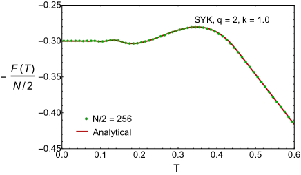
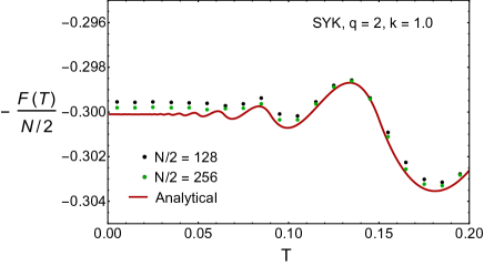
Figure 2: The free energy of the $q=2$ SYK model for $k=0.1$ (top), $k=0.5$ (middle) and $k=1$ (bottom). The dots denote the results obtained by averaging over an ensemble of 1000 configurations for $N/2=128$ (black) and $N/2=256$ (green) Majorana fermions. The right figure is magnification of the left figure. The $N/2=128$ data are only shown in the right figure. The red curve represents the analytical result for the free energy.

We observe that a phase transition occurs at temperatures for which an additional Matsubara frequency enters in the sum of equation (33). This happens for $\frac{\upsilon_{0}}{\pi T}-\frac{1}{2}=m$ ($m$ being non-negative integers) resulting in a series of critical temperatures parameterized by $m$:

$$T_{c,m}=\frac{2\upsilon_{0}/\pi}{2m+1},$$ (34)

where $\upsilon_{0}=v/\sqrt{2}$ according to equation (21). For $T>T_{c,0}$, there are no Matsubara frequency satisfying $0<\omega_{n}<2\upsilon_{0}$, and no more phase transitions can occur.

We re-iterate that, because of the complex-conjugation invariance of the average single-particle spectral density, we have

$$\langle\log Z_{L}\rangle=\langle\log Z_{L}^{*}\rangle,$$ (35)

so that the two-site quenched free energy just doubles that of the one-site and the free energy density remains the same, that is, $F/N=F_{L}/(N/2)$.

To determine the order of the phase transition it is useful to study the first derivative of the free-energy. Indeed, we observe, see figure  3, that it has kinks that point toward a family of second-order phase transitions, each time a new pair of Matsubara frequencies enters in the sum. This can be shown analytically by expanding the free energy around $T_{c,m}$. We find that the contribution at this new critical temperature scales as $\sim(T-T_{c,m})^{2}$ so, as depicted in figure 2, the free energy (33) is smooth around this critical temperature and therefore the transition cannot be of first order. However, one can easily show that the derivative of the free energy is not smooth at $T_{c,m}$ as is also clear from figure 3.

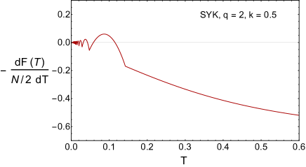
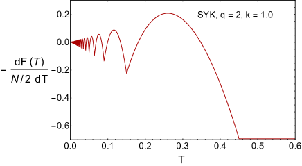
Figure 3: Derivative of the free energy per particle of the non-Hermitian $q=2$ SYK model for $k=0.5$ (left) and $k=1$ (right). The kinks, which indicate the existence of second-order phase transitions, are located at the temperatures (34) where a new Matsubara frequency contributes to the free energy (36). The last kink appears at a temperature $\sim k^{2}$ and would be barely visible for $k=0.1$ which is not shown. The physical scale is set to $v=1$.

Using similar methods, the integrals can also be calculated for $0<k<1$, see appendix B,

$$-\frac{F_{L}}{(N/2)T} = \frac{1}{2}\log 2+\sum_{\omega_{n}\geq 2\upsilon_{0}}^{\infty}\left\{\log\left[\frac{1}{2}\left(1+\sqrt{1+\frac{\epsilon_{0}^{2}-\upsilon_{0}^{2}}{\omega_{n}^{2}/4}}\right)\right]-\frac{1}{2}\frac{\omega_{n}^{2}/4}{\epsilon_{0}^{2}-\upsilon_{0}^{2}}\left(1-\sqrt{1+\frac{\epsilon_{0}^{2}-\upsilon_{0}^{2}}{\omega_{n}^{2}/4}}\right)^{2}\right\}$$ (36)

$$+\frac{1}{2}\sum_{0<\omega_{n}<2\upsilon_{0}}\left\{\log\frac{(\epsilon_{0}+\upsilon_{0})^{2}}{\omega_{n}^{2}}-1-\frac{\omega_{n}^{2}(1-\epsilon_{0}/\upsilon_{0})}{2(\epsilon_{0}^{2}-\upsilon_{0}^{2})}\right\}.$$

Each term contributing to the sum in the first line is equal to the corresponding term in the free energy of the Hermitian SYK model (26) with $\epsilon_{0}\to\sqrt{\epsilon_{0}^{2}-\upsilon_{0}^{2}}$. In figures 2 and 3 we show the temperature dependence of the free energy and its derivative for various values of $k$. It is disturbing that the entropy becomes negative which cannot be due to the failure of the replica trick since it is not used in free-fermion method. Most likely it is a consequence of the nonhermiticity which will become more clear in section V.

The critical temperatures are given by the same expression as for $k=1$,

$$T_{\mathrm{crit}}^{(n)}=\frac{2v_{0}/\pi}{2n+1}\ ,\qquad,n=0,1,2,\cdots$$ (37)

but with $\upsilon_{0}=k^{2}v/\sqrt{1+k^{2}}$ according to equation (21). One can easily show that the derivative of the free energy is continuous at the critical points while its second derivative is discontinuous. The appearance of an infinite number of critical points is a direct consequence of the factorization of the partition function into a product over positive Matsubara frequencies. For each Matsubara frequency we have exactly one critical temperature.

IV Free energy from the Schwinger-Dyson equations

We now turn to confirm these results by an explicit large $N$ calculation from the solutions of the Schwinger-Dyson (SD) equations of the SYK model. In this case, the calculation is also analytical, though very different from the one carried out in the previous section. However, we shall see that ultimately the expression for the free energy is the same. In the Schwinger-Dyson approach, replica symmetry breaking between conjugate replicas plays a crucial role. Indeed, we shall see that for $k=1$ the free energy is determined by the Green’s function $G_{LR}$ (equivalently its self energy $\Sigma_{LR}$) related to the effective coupling of the two sites. However, it is assumed that the replica symmetry of a conjugate pair remains unbroken so that the quenched free energy can be obtained from just one replica and one conjugate replica.

The Euclidean $\Sigma G$ action for the $q$-body SYK model takes the form maldacena2018

$$-\frac{2S_{E}}{N} = \log\mathrm{Pf}(\partial_{t}\delta_{ab}-\Sigma_{ab})-\frac{1}{2}\int d\tau_{1}d\tau_{2}\sum_{a,b}\left[\Sigma_{ab}(\tau_{1},\tau_{2})G_{ab}(\tau_{1},\tau_{2})-s_{ab}\frac{\mathcal{J}_{ab}^{2}}{2q^{2}}[2G_{ab}(\tau_{1},\tau_{2})]^{q}\right]$$ (38)

$$-\frac{i}{2}\epsilon\int d\tau(G_{LR}(\tau,\tau)-G_{RL}(\tau,\tau))\ ,$$

where the indices $a,\,b$ can be equal to $R$ or $L$. The integrations over $\tau$ variables are on the interval $[0,\beta]$. The factor $s_{ab}$ is equal to 1 for $a=b$ and equal to $(-1)^{q/2}=-1$ for $a\neq b$. The couplings take the value ${\mathcal{J}}_{LL}={\mathcal{J}}_{RR}={\mathcal{J}}$ when $a=b$ and ${\mathcal{J}}_{LR}={\mathcal{J}}_{RL}=\mathcal{\widetilde{J}}$ when $a\neq b$. The term proportional to $\epsilon$ is included to break the symmetry that requires $G_{LR}$ to vanish (more details are given in the analysis of the $q=4$ modelGarcia-Garcia:2022 ). In terms of the random coupling couplings of the $L$ and $R$ gamma matrices, $J_{ij}^{L}$ and $J_{ij}^{R}$, for $q=2$ the constants ${\mathcal{J}}$ and $\widetilde{\mathcal{J}}$ are defined by

$$\mathcal{J}^{2}:=\frac{N}{2}\langle(J^{L}_{ij})^{2}\rangle=\frac{N}{2}\langle(J^{R}_{ij})^{2}\rangle=(1-k^{2})v^{2}\ ,$$

$$\widetilde{\mathcal{J}}^{2}:=\frac{N}{2}\langle J^{L}_{ij}J^{R}_{ij}\rangle=(1+k^{2})v^{2}\ ,$$ (39)

where the left and right couplings are related to the couplings $J_{ij}$ and $M_{ij}$ by

$$J^{L}_{ij}\equiv J_{ij}+i\,kM_{ij}\ ,$$

$$J^{R}_{ij}\equiv J_{ij}-i\,kM_{ij}\ .$$ (40)

For a discussion of the symmetries of $G_{ab}\sim\Sigma_{ab}$ we refer to a study of the $q=4$ model Garcia-Garcia:2022 . As it stands the integrals over $\Sigma$ and $G$ for the action (38) are not convergent which is required to perform the integrations over $G_{ab}$. Convergence can be achieved by rotating

$$G_{RR}(\tau_{1},\tau_{2})\to iG_{RR}(\tau_{1},\tau_{2}),\qquad G_{LL}(\tau_{1},\tau_{2})\to iG_{LL}(\tau_{1},\tau_{2})$$

$$\Sigma_{RL}(\tau_{1},\tau_{2})\to i\Sigma_{RL}(\tau_{1},\tau_{2}),\qquad\Sigma_{LR}(\tau_{1},\tau_{2})\to i\Sigma_{LR}(\tau_{1},\tau_{2}).$$ (41)

The rotations do not affect the saddle-point evaluation of the action integral, but as we shall see below, explicitly integrating out $G$ for $q=2$ simplifies the saddle-point analysis and we prefer to use a convergent definition for this reason. The action that gives a convergent path integral is then

$$-\frac{2S_{E}}{N} = \log\mathrm{Pf}(\partial_{\tau}\delta_{ab}-\xi_{ab}\Sigma_{ab})-\frac{1}{2}\int d\tau_{1}d\tau_{2}\sum_{ab}\left[i\Sigma_{ab}(\tau_{1},\tau_{2})G_{ab}(\tau_{1},\tau_{2})+\frac{\mathcal{J}_{ab}^{2}}{2}G_{ab}(\tau_{1},\tau_{2})^{2}\right]$$ (42)

$$-\frac{i}{2}\epsilon\int d\tau(G_{LR}(\tau,\tau)-G_{RL}(\tau,\tau))\ ,$$

with $\xi_{LL}=\xi_{RR}=1$ and $\xi_{LR}=\xi_{RL}=i$. Contrary to $q=4$, the integrals over $G_{ab}(\tau_{1},\tau_{2})$ are Gaussian and can be carried out exactly. This results in the effective action for $\Sigma_{ab}$

$$-\frac{2S_{E}(\Sigma)}{N} = \log\mathrm{Pf}(\partial_{\tau}\delta_{ab}-\xi_{ab}\Sigma_{ab})-\frac{1}{4}\int d\tau_{1}d\tau_{2}\sum_{a,b}\left(\frac{\Sigma_{ab}(\tau_{1},\tau_{2})}{\mathcal{J}_{ab}}\right)^{2}$$ (43)

$$-\frac{1}{2}\epsilon\int d\tau(\Sigma_{LR}(\tau,\tau)-\Sigma_{RL}(\tau,\tau)),\ .$$

At the saddle point, $\Sigma$ should be translation-invariant and hence only a function of $\tau_{1}-\tau_{2}$. For the purpose of saddle-point analysis, we can express the action in terms of Fourier modes of the $\Sigma_{ab}$ which is now a single-variable anti-periodic function:

$$\Sigma_{ab}(\tau) = \frac{1}{\beta}\sum_{\omega_{n}}e^{-i\omega_{n}\tau}\Sigma_{ab}(\omega_{n}),$$ (44)

where $\omega_{n}=(2n+1)\pi/\beta$ are Matsubara frequencies defined already in equation (25). This results in

$$-\frac{2S_{E}(\Sigma)}{N} = \sum_{\omega_{n}}\frac{1}{2}\log\det(-i\omega_{n}\delta_{ab}-\xi_{ab}\Sigma_{ab}(\omega_{n}))-\frac{1}{4}\sum_{ab}\frac{\Sigma_{ab}(\omega_{n})\Sigma_{ab}(-\omega_{n})}{\mathcal{J}_{ab}^{2}}$$ (45)

$$-\frac{1}{2}\epsilon\sum_{\omega_{n}}(\Sigma_{LR}(\omega_{n})-\Sigma_{RL}(\omega_{n}))\ .$$

As already emphasized, contrary to the $q=4$ case, in the $q=2$ case the SD equation simplify to second order equations (we took the limit $\epsilon\to 0$)

$$\frac{i\omega_{n}+\Sigma_{RR}(\omega_{n})}{(i\omega_{n}+\Sigma_{LL}(\omega_{n}))(i\omega_{n}+\Sigma_{RR}(\omega_{n}))+\Sigma_{LR}(\omega_{n})\Sigma_{RL}(\omega_{n})} = \frac{\Sigma_{LL}(-\omega_{n})}{\mathcal{J}^{2}},$$

$$\frac{\Sigma_{RL}(\omega_{n})}{(i\omega_{n}+\Sigma_{LL}(\omega_{n}))(i\omega_{n}+\Sigma_{RR}(\omega_{n}))+\Sigma_{LR}(\omega_{n})\Sigma_{RL}(\omega_{n})} = \frac{\Sigma_{LR}(-\omega_{n})}{\widetilde{\mathcal{J}}^{2}},$$ (46)

and anther two equations with subscripts $L$ and $R$ interchanged. At the saddle point we have that $\Sigma_{RL}(\omega_{n})=-\Sigma_{LR}(\omega_{n})$ and $\Sigma_{RR}(\omega_{n})=\Sigma_{LL}(\omega_{n})$. The saddle point equations couple positive and negative frequencies, but the solutions are simply related by

$$\Sigma_{LL}(-\omega_{n})=-\Sigma_{LL}(\omega_{n}),\qquad\Sigma_{LR}(-\omega_{n})=\Sigma_{LR}(\omega_{n}).$$ (47)

Using these relations the saddle point equations are easily solved with a trivial solution given by (the symmetries of $G_{ab}$ and $\Sigma_{ab}$ are discussed in detail in the analysis of the $q=4$ model Garcia-Garcia:2022 ),

$$\Sigma_{LR}(\omega_{n}) = 0,$$

$$\Sigma_{LL}(\omega_{n}) = -\frac{i}{2}\omega_{n}\pm\frac{i}{2}{\rm sign}(\omega_{n})\sqrt{4\mathcal{J}^{2}+\omega_{n}^{2}},$$ (48)

and a nontrivial solution that couples the Left and Right SYK models breaking the replica symmetry between them:

$$\Sigma_{LR}(\omega_{n}) = \pm\widetilde{\mathcal{J}}\sqrt{1-\frac{\omega_{n}^{2}}{{\omega_{\rm cr}}^{2}}},$$

$$\Sigma_{LL}(\omega_{n}) = \frac{i\mathcal{J}^{2}\omega_{n}}{\widetilde{\mathcal{J}}^{2}-\mathcal{J}^{2}},$$ (49)

where we have introduced the critical frequency

$$\omega_{\rm cr}=\frac{\widetilde{\mathcal{J}}^{2}-\mathcal{J}^{2}}{\widetilde{\mathcal{J}}}\;.$$ (50)

This frequency will play an important role in the analysis of the partition function.

Pairing the positive and negative Matsubara frequencies allows us to write the free energy as a sum over only positive Matsubara frequencies:

$$-\frac{2F}{NT}=\sum_{\omega_{n}>0}\left\{\frac{1}{2}\log\left[\left(i\omega_{n}+\Sigma_{LL}(\omega_{n})\right)^{2}-\Sigma_{LR}(\omega_{n})^{2}\right]^{2}+\frac{\Sigma_{LL}(\omega_{n})^{2}}{\mathcal{J}^{2}}-\frac{\Sigma_{LR}(\omega_{n})^{2}}{\widetilde{\mathcal{J}}^{2}}\right\}.$$ (51)

For unbroken saddles we have two solutions, and it turns out one solution gives a larger $-S_{E}$ hence is the dominant saddle. This is the solution with $+\rm sign(\omega_{n})$ term for $\Sigma_{LL}$. The free energy of this solution is equal to the free energy of two uncoupled SYK models Cotler:2016fpe (but with $\mathcal{J}^{2}=(1-k^{2})v^{2}$). For each (positive) Matsubara frequency this gives

$$-\frac{2F_{\rm\;2\;SYK}(\omega_{n})}{NT}=-\frac{\omega_{n}^{2}}{4\mathcal{J}^{2}}\left(1-\sqrt{1+\frac{4\mathcal{J}^{2}}{\omega_{n}^{2}}}\right)^{2}+\log\left[\frac{1}{4}\left(1+\sqrt{1+\frac{4\mathcal{J}^{2}}{\omega_{n}^{2}}}\right)^{2}\right]+\log(\omega_{n}^{2}),$$

while the free energy of the broken solution reduces to

$$-\frac{2F_{\rm Broken}(\omega_{n})}{NT}=-1+\frac{\omega_{n}^{2}}{\widetilde{\mathcal{J}}^{2}-\mathcal{J}^{2}}+\log\widetilde{\mathcal{J}}^{2}.$$ (53)

The broken solution always gives the dominant action, but as we will see next, it does not always determine the free energy. The saddle point of $\Sigma_{LL}(\omega_{n})$ is always purely imaginary, but the saddle point of $\Sigma_{LR}(\omega_{n})$ switches from real to imaginary at $\omega_{n}=\omega_{\rm cr}$ where the free energy of the trivial and the nontrivial solution coincides. For $\omega_{n}>\omega_{cr}$ the imaginary part of the action is zero at the saddle point, but the action becomes complex along the integration manifold. In order to apply the steepest descent method, the integration manifold must be directed along the Picard-Lefschetz thimble. Otherwise we will have large cancellations that may suppress the action of the saddle point minimizes the the free energy. It is a complicated problem to find the Lefschetz thimbles in a multidimensional space, but we can analyze the problem along the trajectory where $\Sigma_{LL}(\omega_{n})$ and $\Sigma_{RR}(\omega_{n})$ are at the saddle point while for the off-diagonal $\Sigma_{ab}(\omega_{n})$ variables we restrict ourselves to the sub-manifold $\Sigma_{RL}(\omega_{n})=-\Sigma_{LR}(\omega)_{n}$ and $\Sigma_{RL}(-\omega_{n})=-\Sigma_{LR}(\omega_{n})$ which intersects with the saddle-point. Combining positive and negative Matsubara frequencies, the action on this sub-manifold is given by

$$\frac{-2S_{E}(\omega_{n})}{N}=-\frac{\mathcal{J}^{2}\omega_{n}^{2}}{(\widetilde{\mathcal{J}}^{2}-\mathcal{J}^{2})^{2}}-\frac{\Sigma_{LR}^{2}(\omega_{n})}{\widetilde{\mathcal{J}}^{2}}+\log\left(\frac{\widetilde{\mathcal{J}}^{4}\omega_{n}^{2}}{(\widetilde{\mathcal{J}}^{2}-\mathcal{J}^{2})^{2}}+\Sigma_{LR}^{2}(\omega_{n})\right),\qquad\omega_{n}>0.$$

This action also arises in the study of a zero-dimensional Gross-Neveu-like model, and its saddle point analysis Kanazawa:2014qma ; Tanizaki:2015gpl , which we will apply here. The saddle points of this effective action are still given by the $\Sigma_{LR}$ of (IV) and (IV) of the full action, namely $\Sigma_{LR}=0$ and $\Sigma_{LR}(\omega_{n})=\pm\widetilde{\mathcal{J}}\sqrt{1-{\omega_{n}^{2}}/{\omega_{\rm cr}}^{2}}$. At all the saddle points the action is real and the Lefschetz thimble of these saddle points are the real axis if the saddle point solution for $\Sigma_{LR}$ is real, and along the imaginary axis when this saddle point is imaginary. In the the latter case, i.e. for $\omega_{n}>\omega_{\rm cr}$, the thimble ends are the zeros of the logarithm, and it is not possible to deform the real axis continuously into the thimble. Of course we can deform the initial integration over the real axis to an integration path in the complex plane that goes over the saddle point on the imaginary axis. As long as we do not cross any singularities, by Cauchy’s theorem, the value of the integral along the deformed path will be the same in spite of the fact that the integrand at the saddle point on the imaginary axis is much larger than that of the saddle points on the real axis. The phase of the integrand together with the Jacobian will assure that the contributions to the integral combine to the correct result. However, if we integrate only over the Gaussian fluctuations about the imaginary saddle point, we do $not$ get the correct result. In order words, we cannot apply the saddle-point approximation to the imaginary saddle points. Instead, the integral can be evaluated at the trivial saddle point which has its thimble on the real axis. For $\omega_{n}<\omega_{\rm cr}$ the $\Sigma_{LR}(\omega_{n})$ integral runs over both real saddle-points but one of them is suppressed by the $\epsilon$ term in the action.

Strictly speaking, the $\Sigma_{LR}=0$ saddle of the effective action (IV) does not quite correspond to the $\Sigma_{LR}=0$ saddle of the full action, because in writing down the effective action we already assumed a $\Sigma_{LL}$ of the form in solution (IV), but the $\Sigma_{LR}=0$ saddle of the full action belongs to solution (IV) where $\Sigma_{LL}$ takes a different form. Thus $\Sigma_{LR}=0$ solution for the effective action should be viewed as a spurious saddle due to the sub-manifold constraint. Therefore a more definitive analysis should be performed on the full action (the full action is quite similar, though not exactly the same, as the action of a zero-dimensional Nambu-Jona-Lasinio-like model Kanazawa:2014qma ; Tanizaki:2015gpl ). However, our analysis on the sub-manifold is indicative of the inaccessibility of nonzero imaginary $\Sigma_{LR}$ solutions. We thus conclude that

$$\omega_{n} < \omega_{\rm cr}\;:\quad\Sigma_{LR}(\omega_{n})\neq 0\quad\text{(Broken Replica Symmetry)}$$

$$\omega_{n} > \omega_{\rm cr}\;:\quad\Sigma_{LR}(\omega_{n})=0\quad\text{(Replica Diagonal Solution)}$$ (55)

The corresponding partition function is given by

$$F(\omega_{n}<\omega_{\rm cr}) = F_{\rm\;2\;SYK}(\omega_{n}),$$

$$F(\omega_{n}>\omega_{\rm cr}) = F_{\rm\;Broken}(\omega_{n}).$$ (56)

The free energy of the replica diagonal solution is just the free energy of two decoupled SYK models Cotler:2016fpe .

Summing over all Matsubara frequencies we obtain the total free energy

$$F = \sum_{\omega_{\rm cr}>\omega_{n}>0}F_{\rm\;Broken}(\omega_{n})+\sum_{\omega_{n}\geq\omega_{\rm cr}}F_{\;2\;SYK}(\omega_{n})$$ (57)

$$= \sum_{\omega_{n}>0}\log\omega_{n}^{2}+\sum_{\omega_{\rm cr}>\omega_{n}>0}(F_{\rm\;Broken}-\log\omega_{n}^{2})+\sum_{\omega_{n}\geq\omega_{\rm cr}}(F_{\;2\;SYK}-\log\omega_{n}^{2})$$

The first term can be evaluated using zeta function regularization:

$$\sum_{\omega_{n}>0}\log\omega_{n}^{2} = -2\left.\frac{d}{ds}\left[\frac{1}{(2\pi T)^{s}}\sum_{n>0}\frac{1}{(n+1/2)^{s}}\right]\right|_{s=0}$$ (58)

$$= \log 2.$$

This result gives the entropy of noninteracting Majorana particles. Our final expression for the free energy is given by

$$-\frac{2F}{NT} = \log 2+\sum_{\omega_{\rm cr}>\omega_{n}>0}\left\{\frac{\omega_{n}^{2}}{\widetilde{\mathcal{J}}^{2}-\mathcal{J}^{2}}-1+\log\left(\frac{\widetilde{\mathcal{J}}^{2}}{\omega_{n}^{2}}\right)\right\}$$ (59)

$$+\sum_{\omega_{n}\geq\omega_{\rm cr}}\left\{-\frac{\omega_{n}^{2}}{4\mathcal{J}^{2}}\left(1-\sqrt{1+\frac{4\mathcal{J}^{2}}{\omega_{n}^{2}}}\right)^{2}+\log\left[\frac{1}{4}\left(1+\sqrt{1+\frac{4\mathcal{J}^{2}}{\omega_{n}^{2}}}\right)^{2}\right]\right\}.$$

For $k=1$ we have that $\mathcal{J}=0$ and the last term vanishes. We note that the free-fermion expression (36) agrees with (59) after identifying the parameters by

$$\epsilon_{0}^{2}-\upsilon_{0}^{2}=\mathcal{J}^{2},\ (\epsilon_{0}+\upsilon_{0})^{2}=\tilde{\mathcal{J}}^{2},\ 1-\frac{\epsilon_{0}}{\upsilon_{0}}=\frac{2\mathcal{J}^{2}}{\mathcal{J}^{2}-\tilde{\mathcal{J}}^{2}},\ \upsilon_{0}=\frac{\tilde{\mathcal{J}}^{2}-\mathcal{J}^{2}}{2\tilde{\mathcal{J}}}.$$ (60)

The order parameter of the phase transition is given by $\Sigma_{LR}$. In figure 4 we show the analytical result (IV) compared with a numerical calculation for $N/2=256$ that will be discussed in section V.

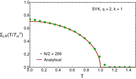
Figure 4: The order parameter $\Sigma_{LR}$ versus the temperature in units of the critical temperature compared to the value of $\Sigma_{LR}$ calculated from the eigenvalues of the hermiticized coupling matrix (see section V).

The $\Sigma$ model that is obtained after integration over the $G$ variables resembles the usual random matrix theory $\sigma$-model. In the next section we will derive basically same the $\sigma$-model directly starting from a partition function that is factorized into a product over Matsubara frequencies.

V Nonlinear $\sigma$-Model for $q=2$ partition function

From equation (16), we can express the partition function of the $q=2$ Hamiltonian as

$$\langle Z\rangle=\left\langle\prod_{k=1}^{N/4}2\cosh\beta\varepsilon_{k}\prod_{k=1}^{N/4}2\cosh\beta\varepsilon_{k}^{*}\right\rangle,$$ (61)

where $\varepsilon_{k}$ are the eigenvalues of $i(J_{ij}+ikM_{ij})/2$ with positive real parts. Using the Weierstrass formula this can rewritten in terms of a product over Matsubara frequencies $\omega_{n}=2\pi(n+\frac{1}{2})/\beta$ :

$$\langle Z\rangle = 2^{N/2}\left\langle\prod_{\omega_{n}>0}\omega_{n}^{-N}\prod_{\pm\varepsilon_{k}}\left(\omega_{n}-2i\varepsilon_{k}\right)\prod_{\pm\varepsilon_{k}}\left(\omega_{n}+2i\varepsilon_{k}^{*}\right)\right\rangle$$ (62)

$$= \left\langle\prod_{\omega_{n}>0}\det\left(\omega_{n}+h\right)\det\left(\omega_{n}+h^{\dagger}\right)\right\rangle,$$

where the product $\prod_{n}\omega_{n}$ has been evaluated to be $\sqrt{2}$ by zeta function regularization (see equation (58)), and $h$ is the $N/2\times N/2$ skew-symmetric matrix $J+ikM$. To leading order in $1/N$ we have

$$\langle Z\rangle=\left\langle\prod_{\omega_{n}>0}Z(\omega_{n})\right\rangle=\prod_{\omega_{n}>0}\langle Z(\omega_{n})\rangle+O(1/N).$$ (63)

Let us first consider a one-site SYK at frequency $\omega_{n}$. The average partition function is given by

$$\langle Z\rangle=\left\langle\prod_{\omega_{n}>0}\det\left(\omega_{n}+h\right)\right\rangle.$$ (64)

The determinant can be expressed Liao:2021ofk as an integral over Grassmann variables $\phi$ and $\phi^{*}$:

$$\langle Z(\omega_{n})\rangle=\left\langle\int\prod_{i}d\phi_{i}d\phi_{i}^{*}e^{\sum_{ij}\phi^{*}_{i}(\omega_{n}\delta_{ij}+h_{ij})\phi_{j}}\right\rangle$$ (65)

We recall that $\langle J_{ij}^{2}\rangle=\langle M_{ij}^{2}\rangle={\cal J}^{2}/(1-k^{2})$, so the Gaussian average over $h$ can be performed by a cumulant expansion resulting in

$$\langle Z(\omega_{n})\rangle = \int\prod_{i}d\phi_{i}d\phi_{i}^{*}e^{\omega_{n}(\phi^{*}\cdot\phi)+\frac{1}{N}{\cal J}^{2}\sum_{i<j}(\phi_{i}^{*}\phi_{j}-\phi_{j}^{*}\phi_{i})^{2}}$$ (66)

$$= \int\prod_{i}d\phi_{i}d\phi_{i}^{*}e^{\omega_{n}(\phi^{*}\cdot\phi)-\frac{1}{N}{\cal J}^{2}\sum_{ij}\phi_{i}^{*}\phi_{j}\phi_{j}^{*}\phi_{i}}$$

$$= \int\prod_{i}d\phi_{i}d\phi_{i}^{*}e^{\omega_{n}(\phi^{*}\cdot\phi)+\frac{1}{N}{\cal J}^{2}(\phi^{*}\cdot\phi)^{2}}$$

where we have used $\phi_{i}^{2}=0$ due to their Grassmannian nature. Using the Hubbard-Stratonovich transformation

$$e^{\alpha^{2}A^{2}/2}=\frac{1}{\sqrt{2\pi\alpha^{2}}}\int d\Sigma e^{-\frac{\Sigma^{2}}{2\alpha^{2}}-\Sigma A}$$ (67)

we obtain

$$\langle Z(\omega_{n})\rangle = \int\prod_{i}d\phi_{i}d\phi_{i}^{*}d\Sigma e^{\omega_{n}(\phi^{*}\cdot\phi)-\frac{N}{4}\frac{\Sigma^{2}}{\mathcal{J}^{2}}-\Sigma(\phi^{*}\cdot\phi)}.$$ (68)

$$= \int d\Sigma\ (\omega_{n}-\Sigma)^{N/2}e^{-\frac{N}{4}\frac{\Sigma^{2}}{\mathcal{J}^{2}}}.$$

The saddle point equation is

$$\Sigma^{2}-\omega_{n}\Sigma-\mathcal{J}^{2}=0.$$ (69)

The dominant solution is given by (we have $\omega_{n}>0$ to start with)

$$\Sigma=\frac{\omega_{n}}{2}-\frac{1}{2}\sqrt{\omega^{2}_{n}+4\mathcal{J}^{2}}.$$ (70)

with leads to the one-site free energy

$$-\frac{F(\omega_{n})}{TN/2}=\log\left(\frac{\omega_{n}}{2}+\frac{1}{2}\sqrt{\omega_{n}^{2}+4\mathcal{J}^{2}}\right)-\frac{1}{2\mathcal{J}^{2}}\left(\frac{\omega_{n}}{2}-\frac{1}{2}\sqrt{\omega_{n}^{2}+4\mathcal{J}^{2}}\right)^{2}.$$ (71)

This is exactly half of the the Schwinger-Dyson result for the two-site model using only the replica-symmetric saddles. The total free energy is given by

$$-\frac{F}{TN/2}=\sum_{\omega_{n}>0}-\frac{F_{\;2\;SYK}(\omega_{n})}{TN}.$$ (72)

This shows explicitly that the one-site annealed partition function gives the quenched result for the high-temperature phase of the of the nonhermitian SYK model as is the case for the $q=4$ SYK model. For $T<T_{c}$ the replica limit of the one-site partition function fails to give the quenched result. In order to get the correct result we have to take the replica limit of the partition function and the conjugate partition function, which is well-known from the $\sigma$-model formulation of nonhermitian random matrix theories girko2012theory ; efetov1997directed ; feinberg1997non and QCD at nonzero chemical potential stephanov1996 ; Janik:1996va ; Janik:1996xm ; splittorff:2003cu .

Next we consider the two-site non-Hermitian model and also assume that the ensemble average factorizes in the large $N$ limit so that we can evaluate the partition function for a single frequency

$$\langle Z(\omega_{n})\rangle = \left\langle\det\big{(}\omega_{n}+h\big{)}\det\big{(}\omega_{n}+h^{\dagger}\big{)}\right\rangle,$$ (73)

$$= \int\left(\prod_{i}^{N/2}d\phi^{i}_{L}d\phi^{i*}_{L}d\phi^{i}_{R}d\phi^{i*}_{R}\right)e^{\phi_{L}^{*}\cdot(\omega_{n}+h)\cdot\phi_{L}+\phi_{R}^{*}\cdot(\omega_{n}+h^{\dagger})\cdot\phi_{R}}.$$

We can again average over $h$ by a cumulant expansion using that

$$\langle h_{ij}^{2}\rangle = \langle h_{ij}^{2}\rangle=\frac{{\cal J}^{2}}{N/2},$$

$$\langle h_{ij}h_{ij}^{*}\rangle = \frac{\widetilde{\cal J}^{2}}{N/2}.$$ (74)

This results in the quartic action

$$-S_{4}=\frac{\mathcal{J}^{2}}{N}\left[(\phi_{R}^{*}\cdot\phi_{R})^{2}+(\phi_{L}^{*}\cdot\phi_{L})^{2}\right]+\frac{2\widetilde{\mathcal{J}}^{2}}{N}\left[(\phi_{L}^{*}\cdot\phi_{R}^{*})(\phi_{L}\cdot\phi_{R})+(\phi_{L}^{*}\cdot\phi_{R})(\phi_{L}\cdot\phi_{R}^{*})\right].$$ (75)

This action is invariant under

$$\phi_{L}\to e^{i\varphi}\phi_{L},\qquad\phi_{R}\to e^{i\psi}\phi_{R}.$$ (76)

In addition to the Hubbard-Stratonovich transformation (67) we use the identity

$$e^{\alpha^{2}AA^{*}}\sim e^{-\frac{\Sigma\Sigma^{*}}{\alpha^{2}}-\Sigma A^{*}-\Sigma^{*}A}$$ (77)

to decouple the quartic terms. This results in

$$Z(\omega_{n})=\int d\Sigma d\rho e^{-\frac{N}{4\mathcal{J}^{2}}\left[\Sigma_{RR}^{2}+\Sigma_{LL}^{2}\right]-\frac{N}{2\widetilde{\mathcal{J}}^{2}}\left[\Sigma^{*}_{LR}\Sigma_{LR}+\rho_{LR}\rho_{LR}^{*}\right]}I^{N/2}(\{\Sigma,\rho\}),$$ (78)

where $d\Sigma=d\Sigma_{LL}d\Sigma_{RR}d\Sigma_{LR}d\Sigma^{*}_{LR}$ and $d\rho=d\rho_{LR}d\rho^{*}_{LR}$ and we have used that the integral over the $\phi^{i}_{a}$ variables factorizes into a product over $I$. Each of these factors is equal to

$$I = \int d\phi_{L}d\phi^{*}_{L}d\phi_{R}d\phi^{*}_{R}\exp[(\omega_{n}-\Sigma_{LL})\phi_{L}^{*}\phi_{L}+(\omega_{n}-\Sigma_{RR})\phi_{R}^{*}\phi_{R}$$ (79)

$$\hskip 113.81102pt-\Sigma_{LR}\phi_{L}^{*}\phi_{R}-\Sigma_{LR}^{*}\phi_{L}\phi_{R}^{*}-\rho_{LR}\phi_{L}^{*}\phi_{R}^{*}-\rho_{LR}^{*}\phi_{L}\phi_{R}],$$

where the $\phi_{a}$ no longer carry an index $i$. This integral can be evaluated by simply expanding the exponential in the integrand and collecting the terms that are proportional to $\phi_{L}\phi^{*}_{L}\phi_{R}\phi^{*}_{R}$. We get

$$I=(\omega_{n}-\Sigma_{LL})(\omega_{n}-\Sigma_{RR})+\Sigma_{LR}^{*}\Sigma_{LR}-\rho_{LR}^{*}\rho_{LR}.$$ (80)

The saddle points can be grouped in to the following three classes:

$$\rho_{LR}=0,\quad\Sigma_{LR}=0,\quad\Sigma_{LL}=\Sigma_{RR}=\frac{\omega_{n}}{2}-\frac{1}{2}\rm sign(\omega_{n})\sqrt{\omega_{n}^{2}+4\mathcal{J}^{2}},$$ (81)

$$\rho_{LR}=0,\quad|\Sigma_{LR}|^{2}=\widetilde{\mathcal{J}}^{2}\left(1-\frac{\omega_{n}^{2}}{\omega_{\rm cr}^{2}}\right),\quad\Sigma_{LL}=\Sigma_{RR}=-\frac{\mathcal{J}^{2}\omega_{n}}{\widetilde{\mathcal{J}}^{2}-\mathcal{J}^{2}},$$ (82)

$$|\rho_{LR}|^{2}=\widetilde{\mathcal{J}}^{2}\left[1+\frac{\widetilde{\mathcal{J}}^{2}\omega_{n}^{2}}{(\widetilde{\mathcal{J}}^{2}+\mathcal{J}^{2})^{2}}\right],\quad\Sigma_{LR}=0,\quad\Sigma_{LL}=\Sigma_{RR}=-\frac{\mathcal{J}^{2}\omega_{n}}{\widetilde{\mathcal{J}}^{2}+\mathcal{J}^{2}}.$$ (83)

Now the first two saddles are simply the ones we found in the SD equations in section IV, and if the third saddle can be discarded they would reproduce the same saddle-point analysis, which we recall here: although the second saddle (symmetry-breaking saddle) has a dominant action (larger $-S_{E}$) for all values of $\omega_{n}$, thimble analysis requires us to pick the second saddle only for $\omega_{n}<\omega_{\rm cr}$ and for $\omega_{n}>\omega_{\rm cr}$ we must pick the first saddle (unbroken saddle). Let us now show why the third saddle can be discarded: the third saddle’s action ($-S_{E}$) is smaller than that of the second saddle for all $\omega_{n}$, so we do not need to worry about it for $\omega_{n}<\omega_{\rm cr}$; its action is smaller than that of the first saddle for $\omega_{n}>\omega_{\rm cr}$ (its action can be larger than that of the first saddle only for $\omega_{n}<\omega_{\rm cr}$), hence we do not need to worry about the third saddle for $\omega_{n}>\omega_{\rm cr}$ either. Thus, the third saddle drops out of our consideration for all values of $\omega_{n}$ and we reproduce the same free energy found in section IV.

The order parameter of the phase transition of the coupled SYK model is given by the expectation value of $\Sigma_{LR}$. This is equal to

$$\langle\Sigma_{LR}\rangle=-\frac{2\widetilde{\mathcal{J}}^{2}}{N}\langle\phi_{L}\cdot\phi_{R}^{*}\rangle$$ (84)

This is the chiral condensate corresponding to the spectral density of

$${\cal H}=\left(\begin{array}[]{cc}0&h+\omega_{n}\\ h^{\dagger}+\omega_{n}&0\end{array}\right).$$ (87)

It is given by the Banks-Casher formula Banks:1979yr

$$\Sigma_{LR}=-\lim_{\epsilon\to 0}\lim_{N\to\infty}\frac{2\widetilde{\mathcal{J}}^{2}}{N}\textrm{Tr}\frac{1}{{\cal H}+i\epsilon}=\lim_{N\to\infty}\frac{\pi\rho_{\cal H}(0)}{N}.$$ (88)

The critical temperature is determined by the value of $\omega_{n}$ at which a gap opens and the spectrum becomes gapped for $T>T_{c}$. Another interpretation of the critical temperature is that $T_{c}$ is the point at which $\omega_{n}$ enters the spectral support of $h$. The spectral density of ${\cal H}$ can be obtained analytically and follows from the solution of a cubic equation Jackson:1995nf ; Jackson:1996xt . The phase transition is a typical Landau-Ginsberg phase transition with mean field critical exponents.

The partition function $Z(\omega_{n})$ with $h$ replaced by a complex matrix was first introduced as a random matrix model for chiral symmetry breaking in QCD Jackson:1995nf and further analytical results were obtained in a subsequent paper Jackson:1996xt .

VI Outlook and conclusions

In conclusion, the free energy of the integrable $q=2$ SYK model is qualitatively different from the $q>2$ case. Not only is the order of the transition is different, but also there is an infinite series of transitions while for $q>2$ there is only one. This goes back to the factorization of partition function into a product over Matsubara frequencies. Each of the factors undergoes a phase transition from a replica symmetric solution to a solution with broken replica symmetry with a critical temperature that depends on the Matsubara frequency. For the full partition function this results into an infinite sequence of phase transitions.

We have calculated the quenched free energy in two structurally different ways. First, a quenched calculation based on the free-fermion description of the $q=2$ SYK model, and second, an annealed calculation based on the solution of the Schwinger-Dyson equations in the $\Sigma G$ formulation of the SYK model using the replica trick. The two methods give the same result which shows that despite the nonhermiticity of the model, the replica limit gives the correct result provided that the starting point is the product of the one-site partition function and its complex conjugate before averaging. On the other hand, in the quenched free-fermion calculation, we did start from the one-site partition function without having to include the conjugate partition function. The reason this gives the correct result is the factorization of the partition function in a product over single particle energies.

The $q=4$ nonhermitian SYK model behaves quite differently. It is not a Fermi liquid and the usual free-fermion description is invalid which is most notable in the zero temperature entropy which is extensive Sachdev:2001 . The nonhermitian two-site $q=4$ SYK model has a single first order phase transition which separates a low-temperature phase from a high-temperature phase. The high-temperature phase is entropy dominated while the low-temperature phase is energy dominated. The free energy in the high-temperature phase follows from the many-body eigenvalue density and is entirely determined by the one-site partition function. This is also the case for the $q=2$ SYK model. In the low-temperature phase, the replica limit of the one-site partition function breaks down and the quenched one-site partition function is given by the replica limit of the one-site partition function and its complex conjugate. In terms of the many-body spectral density, the two-point spectral correlation function determines the free-energy of the low-temperature phase. For this reason there is large difference between the $q=4$ case and the $q=2$ case. The dynamics of the $q=4$ partition function is chaotic with universal eigenvalue correlations given by the Ginibre model, which as a consequence gives rise to a temperature-independent free energy in the low-temperature phase. On the other hand, the $q=2$ SYK model is integrable with mostly but not entirely uncorrelated eigenvalues. We can distinguish two contributions from the two-point correlation function. One contribution is due to self-correlations, and the second one is due to the many-body correlation resulting from the fact that the $2^{N/2}$ many-body eigenvalues are determined by $N/2$ single-particle energies. It is simple to evaluate the contribution from the self-correlations but this only reproduces the free-energy at zero temperature and is smooth as a function of the temperature. This implies that the infinite series of second-order phase transitions are due to correlations of the many-body eigenvalues.

The phase transitions of the $q=2$ nonhermitian SYK model can also be understood in terms of the spectral properties of the coupling matrix. Using a random matrix theory like $\sigma$-model calculation we have related the order parameter of the phase transition $\Sigma_{LR}$ to the formation of a gap of the hermiticized two-site Hamiltonian. In terms of the one-site Hamiltonian, this is the point where the Matsubara frequency enters the support of the spectrum of $H_{L}$. The starting point of the $\sigma$-model calculation is closely related to a random matrix model for the chiral phase transition in QCD where $\Sigma_{LR}$ plays the role of the chiral condensate.

A natural question is whether the free energy of the $q=2$ SYK model can also be understood in terms of the many-body spectral density and the many-body spectral correlations. The cancellations that are responsible for the high-temperature phase of the $q=4$ model are still at work for $q=2$. For example, at high temperatures and for maximum nonhermiticity the free energy of the $q=2$ SYK model and the $q=4$ SYK model is the same ($-\frac{T}{2}\log 2$ per particle). From the solutions of the SD equations it is clear that the two-point correlation function determines the low-temperature phase. In particular, the transitions observed in the low-temperature phase are due to the coupling between left and right sites but not by the dynamics within each of the sites.

In conclusion, the nature of the quantum dynamics plays a role for the replica symmetry breaking mechanism which also induces phase transitions for the $q=2$ nonhermitian SYK model. However, while the replica dynamics of quantum chaotic systems is universal, there is a broad variety of dynamical behavior associated with integrable systems, and we cannot conclude that the behavior we have observed for the nonhermitian $q=2$ SYK model is generic.

Appendix A Free-fermion representation of the $q=2$ SYK model

We write the $q=2$ one-site Hamiltonian as

$$H_{L}=\frac{1}{2}\sum_{ij}W_{ij}\gamma_{i}\gamma_{j}=\frac{1}{2}\vec{\gamma}^{T}W\vec{\gamma}.$$ (89)

where gamma matrices $\vec{\gamma}=(\gamma_{1},\gamma_{2},\ldots,\gamma_{M})$ with even $M$ and $W$ is a random antisymmetric complex matrix. In the main text we have the convention that $M=N/2$. By matching with definitions (II) and (7), we know

$$W=\frac{1}{2}i(J_{ij}+ikM_{ij}).$$ (90)

In the Hermitian SYK model ($k=0$), $W$ is an antisymmetric Hermitian matrix, and the Hamiltonian can be transformed into a fermion-filling form thanks to the fact that an $M$-dimensional antisymmetric Hermitian matrix has the normal form

$$O\begin{pmatrix}i\varepsilon_{1}\sigma_{2}&0&\cdots&0\\ 0&i\varepsilon_{2}\sigma_{2}&\cdots&\vdots\\ \vdots&\cdots&\cdots&\vdots\\ 0&\cdots&\cdots&i\varepsilon_{\frac{M}{2}}\sigma_{2}\end{pmatrix}O^{T},$$ (91)

where $O$ is a real orthogonal matrix. Using a new basis for the $\gamma$ matrices defined by $O^{T}\vec{\gamma}$, one can easily write the Hermitian Hamiltonian in a fermion-filling form. Although a generic complex antisymmetric matrix does not have a normal form of equation (91), there exists a parallel of it which allows us to write the non-Hermitian Hamiltonian (89) in a modified fermion-filling form. We will demonstrate this now.

We consider a diagonalizable complex antisymmetric matrix $W$ with all eigenvalues being nonzero, which is almost always the case for our ensemble. The eigenvalues of $W$ come in opposite pairs $\pm\varepsilon$, so we can diagonalize $W$ as

$$W=S\Lambda S^{-1},$$ (92)

where

$$\Lambda=\begin{pmatrix}\varepsilon_{1}\sigma_{3}&0&\cdots&0\\ 0&\varepsilon_{2}\sigma_{3}&\cdots&\vdots\\ \vdots&\cdots&\cdots&\vdots\\ 0&\cdots&\cdots&\varepsilon_{\frac{M}{2}}\sigma_{3}\end{pmatrix}.$$ (93)

The column vectors of $S$ are the eigenvectors of $W$, namely

$$S=\begin{pmatrix}\vline&\vline&\cdots&\vline&\vline\\ \vline&\vline&\cdots&\vline&\vline\\ v_{1}&v_{2}&\cdots&v_{M-1}&v_{M}\\ \vline&\vline&\cdots&\vline&\vline\\ \vline&\vline&\cdots&\vline&\vline\\ \end{pmatrix},$$ (94)

where

$$Wv_{2k-1}=\varepsilon_{k}v_{2k-1},\quad Wv_{2k}=-\varepsilon_{k}v_{2k}.$$ (95)

To completely fix the sign convention, we choose $\varepsilon_{k}\ (k=1,\ldots,M/2)$ to have a positive real part. Because $W^{T}=-W$, we have

$$0=v_{i}^{T}\left(W+W^{T}\right)v_{j}=(\varepsilon_{i}+\varepsilon_{j})v_{i}^{T}v_{j}$$ (96)

which implies

$$v_{i}^{T}v_{j}=0\text{ unless }\{i,j\}=\{2k-1,2k\}.$$ (97)

So if we scale the eigenvectors to redefine $S$ as

$$S=\begin{pmatrix}\vline&\vline&\cdots&\vline&\vline\\ \vline&\vline&\cdots&\vline&\vline\\ \frac{v_{1}}{\sqrt{v_{1}^{T}v_{2}}}&\frac{v_{2}}{\sqrt{v_{1}^{T}v_{2}}}&\cdots&\frac{v_{D-1}}{\sqrt{v_{M-1}^{T}v_{M}}}&\frac{v_{M}}{\sqrt{v_{M-1}^{T}v_{M}}}\\ \vline&\vline&\cdots&\vline&\vline\\ \vline&\vline&\cdots&\vline&\vline\\ \end{pmatrix},$$ (98)

we can easily see

$$S^{T}S=\begin{pmatrix}\sigma_{1}&0&\cdots&0\\ 0&\sigma_{1}&\cdots&\vdots\\ \vdots&\cdots&\cdots&\vdots\\ 0&\cdots&\cdots&\sigma_{1}\end{pmatrix}\equiv\Sigma_{1},$$ (99)

and hence $S^{-1}=\Sigma_{1}S^{T}$ (note in general $S^{T}S\neq SS^{T}$). Substituting this into equation (92), we obtain

$$W=S\Lambda\Sigma_{1}S^{T}=S\begin{pmatrix}i\varepsilon_{1}\sigma_{2}&0&\cdots&0\\ 0&i\varepsilon_{2}\sigma_{2}&\cdots&\vdots\\ \vdots&\cdots&\cdots&\vdots\\ 0&\cdots&\cdots&i\varepsilon_{\frac{M}{2}}\sigma_{2}\end{pmatrix}S^{T}.$$ (100)

We thus arrive at a normal form for complex antisymmetric matrices rather similar to that of the Hermitian antisymmetric ones (91), with the difference that $S$ is not orthogonal but satisfies $S^{T}S=\Sigma_{1}$. Now we define new set of operators $\{\tilde{c}_{k},c_{k}|k=1,2\ldots M/2\}$ by

$$\tilde{c}_{k}=\frac{1}{\sqrt{2}}\left(S^{T}\vec{\gamma}\right)_{2k-1},\quad c_{k}=\frac{1}{\sqrt{2}}\left(S^{T}\vec{\gamma}\right)_{2k}.$$ (101)

From the anti-commutation relation of $\gamma$ matrices we derive

$$\frac{1}{2}\left\{\left(S^{T}\vec{\gamma}\right)_{m},\left(S^{T}\vec{\gamma}\right)_{n}\right\}=(\Sigma_{1})_{mn}.$$ (102)

This in particular implies

$$\tilde{c}_{k}^{2}=0,\quad,c_{k}^{2}=0,\quad\{c_{k},\tilde{c}_{l}\}=\delta_{kl}.$$ (103)

Note this is just the algebra for the ladder operators of $M/2$ spinless fermions, except that $c_{k}$ and $\tilde{c}_{k}$ are not related by a Hermitian conjugation. In terms of these ladder operators, the Hamiltonian (89) becomes

$$H=\sum_{k=1}^{M/2}\varepsilon_{k}(2\tilde{c}_{k}c_{k}-1).$$ (104)

Just as the in Hermitian case, we have

$$[H,\tilde{c}_{k}]=\varepsilon_{k}\tilde{c}_{k},\quad[H,c_{k}]=-\varepsilon_{k}c_{k}.$$ (105)

Hence we conclude the many-body energies of $H$ are given by the filling of $M/2$ free fermions into the particle-hole symmetric levels of $W$: each fermion either occupies a “particle” level with energy $\varepsilon_{k}$, or occupies a ”hole” level with energy $-\varepsilon_{k}$. However since the raising and lowering operators are not Hermitian conjugate to each other, the eigenstates are not necessarily orthogonal to each other (at least not with the original inner product $\langle x,y\rangle\equiv x^{\dagger}y$), just as one would expect for a non-Hermitian Hamiltonian.

Appendix B Free energy from the free-fermion representation for $k<1$

Based on the free-fermion representation of the $q=2$ SYK model of appendix A, we proceed to the explicit analytical calculation of the free energy. The simpler spherical case $k=1$ was already discussed in the main text. The free energy for $k<1$ can be derived along the same lines which is the purpose of this appendix.

For $k<1$ ($\upsilon_{0}<\epsilon_{0}$), the large-$N$ single-particle spectral density becomes a constant inside an elliptical disk as in equation (20). The elliptical disk can be parameterized by

$$z=\epsilon_{0}r\cos\phi+i\upsilon_{0}r\sin\phi,\quad r\in[0,1],\;\phi\in[0,2\pi].$$ (106)

We write

$$-\frac{F_{L}}{(N/4)T}=\int_{0}^{1}rI_{E}(r)dr,$$ (107)

where

$$I_{E}(r)=\frac{1}{\pi}\int_{0}^{2\pi}\log\left(2\cosh\frac{\epsilon_{0}r\cos\phi+i\upsilon_{0}r\sin\phi}{T}\right)d\phi.$$ (108)

The subscript $E$ denotes “Ellipse”. On its face, we cannot interpret $I_{E}(r)$ as a complex contour integral like equation (28), because $dz/(iz)\neq d\phi$ with the elliptical parameterization (106). We can overcome this by considering the following conformal (Joukowski) transformation :

$$z=au+\frac{b}{u},$$ (109)

where

$$\quad a=\frac{\epsilon_{0}+\upsilon_{0}}{2}r,\quad b=\frac{\epsilon_{0}-\upsilon_{0}}{2}r.$$ (110)

In terms $u$, the ellipse in equation (106) at any given $r$ becomes a unit circle:

$$u=e^{i\phi}$$ (111)

We stress that the $\phi$ here is the same $\phi$ as in the parameterization (106). Now we can write

$$\begin{split}I_{E}(r)=&\frac{1}{\pi i}\oint_{S^{1}}\frac{du}{u}\log\left(2\cosh\frac{au+b/u}{T}\right)\\ =&2\log 2+\sum_{n=0}^{\infty}\frac{1}{\pi i}\oint_{S^{1}}\frac{du}{u}\log\left(1+\frac{4(au+b/u)^{2}}{\omega_{n}^{2}}\right)\\ \equiv&2\log 2+\sum_{n=0}^{\infty}I_{nE}(r),\end{split}$$ (112)

where to obtain second equality we applied Weierstrass factorization just as we did in the circular case and the third equality simply defines $I_{nE}$. Notice $S^{1}$ denotes the unit circle and the $r$-dependence of the integral comes from the $r$-dependence of $a$ and $b$.

To analyze the cut and pole structures of the integral $I_{nE}$, we rewrite its integrand as

$$\begin{split}\frac{1}{u}\log\left(1+\frac{4(au+b/u)^{2}}{\omega_{n}^{2}}\right)=\frac{1}{u}\log\left[\frac{4a^{2}}{\omega_{n}^{2}u^{2}}(u-u_{1+})(u-u_{1-})(u-u_{2+})(u-u_{2-})\right],\end{split}$$ (113)

where $u_{1\pm},u_{2\pm}$ are the four roots of the equation

$$1+\frac{4(au+b/u)^{2}}{\omega_{n}^{2}}=0,$$ (114)

namely

$$u_{1\pm}=\pm i\frac{\sqrt{\omega_{n}^{2}/4+4ab}-\omega_{n}/2}{2a},\quad u_{2\pm}=\pm i\frac{\sqrt{\omega_{n}^{2}/4+4ab}+\omega_{n}/2}{2a}.$$ (115)

Note that $4ab=(\epsilon_{0}^{2}-\upsilon_{0}^{2})r^{2}>0$, and since $a>b$, $u_{1\pm}$ are always inside the unit circle. We also note that for $u=e^{i\phi}$

$$\oint_{S^{1}}du\frac{\log u}{u}=0.$$ (116)

Hence

$$I_{nE}=\frac{1}{\pi i}\oint_{S^{1}}\frac{du}{u}\log\left[\frac{4a^{2}}{\omega_{n}^{2}}(u-u_{1+})(u-u_{1-})(u-u_{2+})(u-u_{2-})\right].$$ (117)

The integrand of $I_{nE}$ has one pole at the origin with the residue

$$\log\left[\frac{4a^{2}}{\omega_{n}^{2}}u_{1+}u_{1-}u_{2+}u_{2-}\right]=\log\left(\frac{4b^{2}}{\omega_{n}^{2}}\right).$$ (118)

The integrand of $I_{nE}$ has four branch cuts emanating from $u_{1\pm},u_{2\pm}$ horizontally to negative infinity. The $u_{1\pm}$ cuts always intersect with the unit circle, whereas $u_{2\pm}$ may or may not intersect with the unit circle depending on the values of $a$ and $b$. To summarize, the $u_{2\pm}$ cuts contribute to $I_{nE}$ only if $|u_{2\pm}|<1$ (which is to say $r>\omega_{n}/2\upsilon_{0}$), in much the same way as the $\pm i\omega_{n}/2\upsilon_{0}$ cuts contribute to $I_{n}$ in the circular case; what is new with the elliptical case are the $u_{1\pm}$ cuts and the pole at the origin, which always contribute to $I_{nE}$ regardless the value of $r$. Recycling the calculation done in the circular case, we obtain

$$I_{nE}(r)=2\log\left[\frac{1}{4}\left(1+\sqrt{1+\frac{4(\epsilon_{0}^{2}-\upsilon_{0}^{2})r^{2}}{\omega_{n}^{2}}}\right)^{2}\right]$$ (119)

if $r<\omega_{n}/2\upsilon_{0}$. which is the sum of one pole and two cut contributions. And

$$I_{nE}(r)=2\log\left[\frac{1}{4}\left(1+\sqrt{1+\frac{4(\epsilon_{0}^{2}-\upsilon_{0}^{2})r^{2}}{\omega_{n}^{2}}}\right)^{2}\right]+2\log\left(\frac{2(\epsilon_{0}+\upsilon_{0})r}{\omega_{n}+\sqrt{\omega_{n}^{2}+4(\epsilon_{0}^{2}-\upsilon_{0}^{2})r^{2}}}\right)$$ (120)

if $r>\omega_{n}/2\upsilon_{0}$, which is the sum of one pole and four cut contributions. With these results, we arrive at

$$\begin{split}-\frac{F_{L}}{(N/4)T}=&\log 2+\sum_{\omega_{n}>0}\int_{0}^{1}rI_{nE}(r)dr\\ &=\log 2+\sum_{n=0}^{\infty}\left\{\log\left[\frac{1}{4}\left(1+\sqrt{1+\frac{\epsilon_{0}^{2}-\upsilon_{0}^{2}}{\omega_{n}^{2}/4}}\right)^{2}\right]-\frac{\omega_{n}^{2}/4}{\epsilon_{0}^{2}-\upsilon_{0}^{2}}\left(1-\sqrt{1+\frac{\epsilon_{0}^{2}-\upsilon_{0}^{2}}{\omega_{n}^{2}/4}}\right)^{2}\right\}\\ &\qquad-\sum_{0<\omega_{n}<2\upsilon_{0}}\left\{\frac{2\omega_{n}^{2}/4}{\epsilon_{0}^{2}-\upsilon_{0}^{2}}\sqrt{1+\frac{\epsilon_{0}^{2}-\upsilon_{0}^{2}}{\omega_{n}^{2}/4}}+\log\left[\frac{\omega_{n}^{2}/4}{(\epsilon_{0}+\upsilon_{0})^{2}}\left(1+\sqrt{1+\frac{\epsilon_{0}^{2}-\upsilon_{0}^{2}}{\omega_{n}^{2}/4}}\right)^{2}\right]\right\}\\ &\qquad+\sum_{0<\omega_{n}<2\upsilon_{0}}\frac{2\omega_{n}^{2}\epsilon_{0}/4}{(\epsilon_{0}^{2}-\upsilon_{0}^{2})\upsilon_{0}}\\ =&\log 2+\sum_{\omega_{n}>2\upsilon_{0}}\left\{\log\left[\frac{1}{4}\left(1+\sqrt{1+\frac{\epsilon_{0}^{2}-\upsilon_{0}^{2}}{\omega_{n}^{2}/4}}\right)^{2}\right]-\frac{\omega_{n}^{2}/4}{\epsilon_{0}^{2}-\upsilon_{0}^{2}}\left(1-\sqrt{1+\frac{\epsilon_{0}^{2}-\upsilon_{0}^{2}}{\omega_{n}^{2}/4}}\right)^{2}\right\}\\ &\qquad+\sum_{0<\omega_{n}<2\upsilon_{0}}\left\{\log\frac{(\epsilon_{0}+\upsilon_{0})^{2}}{\omega_{n}^{2}}-1-\frac{\omega_{n}^{2}(1-\epsilon_{0}/\upsilon_{0})}{2(\epsilon_{0}^{2}-\upsilon_{0}^{2})}\right\}.\end{split}$$ (121)

The result on the last line exactly matches with the SD calculation provided that

$$\epsilon_{0}^{2}-\upsilon_{0}^{2}=\mathcal{J}^{2},\ (\epsilon_{0}+\upsilon_{0})^{2}=\tilde{\mathcal{J}}^{2},\ 1-\frac{\epsilon_{0}}{\upsilon_{0}}=\frac{2\mathcal{J}^{2}}{\mathcal{J}^{2}-\tilde{\mathcal{J}}^{2}},\ \upsilon_{0}=\frac{\tilde{\mathcal{J}}^{2}-\mathcal{J}^{2}}{2\tilde{\mathcal{J}}}.$$ (122)

References

- (1) F.J. Dyson et al., Selected papers of Freeman Dyson with commentary, vol. 5, American Mathematical Soc. (1996).
- (2) F.J. Dyson, A class of matrix ensembles, J. Math. Phys. 13 (1972) 90.
- (3) H.A. Bethe, An attempt to calculate the number of energy levels of a heavy nucleus, Phys. Rev. 50 (1936) 332.
- (4) J. French and S. Wong, Validity of random matrix theories for many-particle systems, Physics Letters B 33 (1970) 449 .
- (5) J. French and S. Wong, Some random-matrix level and spacing distributions for fixed-particle-rank interactions, Physics Letters B 35 (1971) 5 .
- (6) O. Bohigas and J. Flores, Two-body random hamiltonian and level density, Physics Letters B 34 (1971) 261 .
- (7) O. Bohigas and J. Flores, Spacing and individual eigenvalue distributions of two-body random hamiltonians, Physics Letters B 35 (1971) 383 .
- (8) K. Mon and J. French, Statistical properties of many-particle spectra, Annals of Physics 95 (1975) 90 .
- (9) A. Kitaev, A simple model of quantum holography, KITP strings seminar and Entanglement 2015 program, 12 February, 7 April and 27 May 2015, http://online.kitp.ucsb.edu/online/entangled15/ (2015) .
- (10) J. Maldacena and D. Stanford, Remarks on the Sachdev-Ye-Kitaev model, Phys. Rev. D 94 (2016) 106002 [1604.07818].
- (11) S. Sachdev and J. Ye, Gapless spin-fluid ground state in a random quantum heisenberg magnet, Phys. Rev. Lett. 70 (1993) 3339.
- (12) S. Sachdev, Bekenstein-hawking entropy and strange metals, Phys. Rev. X 5 (2015) 041025.
- (13) E. Wigner, On the statistical distribution of the widths and spacings of nuclear resonance levels, Math. Proc. Cam. Phil. Soc. 49 (1951) 790.
- (14) M.L. Mehta and M. Gaudin, On the density of eigenvalues of a random matrix, Nuclear Physics 18 (1960) 420.
- (15) F.J. Dyson, Statistical theory of the energy levels of complex systems. I, J. Math. Phys. 3 (1962) 140.
- (16) F.J. Dyson, Statistical theory of the energy levels of complex systems. ii, Journal of Mathematical Physics 3 (1962) 157.
- (17) F.J. Dyson, Statistical theory of the energy levels of complex systems. iii, Journal of Mathematical Physics 3 (1962) 166.
- (18) F.J. Dyson and M.L. Mehta, Statistical theory of the energy levels of complex systems. iv, Journal of Mathematical Physics 4 (1963) 701.
- (19) M.L. Mehta and F.J. Dyson, Statistical theory of the energy levels of complex systems. v, Journal of Mathematical Physics 4 (1963) 713.
- (20) F.J. Dyson, The threefold way. algebraic structure of symmetry groups and ensembles in quantum mechanics, Journal of Mathematical Physics 3 (1962) 1199.
- (21) T. Guhr, A. Muller-Groeling and H.A. Weidenmuller, Random matrix theories in quantum physics: Common concepts, Phys. Rept. 299 (1998) 189 [cond-mat/9707301].
- (22) J. Ginibre, Statistical ensembles of complex, quaternion, and real matrices, Journal of Mathematical Physics 6 (1965) 440.
- (23) J.J.M. Verbaarschot, H.A. Weidenmüller and M.R. Zirnbauer, Grassmann integration and the theory of compound-nucleus reactions, Phys. Lett. B 149 (1984) 263.
- (24) J.J.M. Verbaarschot, H.A. Weidenmuller and M.R. Zirnbauer, Grassmann Integration in Stochastic Quantum Physics: The Case of Compound Nucleus Scattering, Phys. Rept. 129 (1985) 367.
- (25) H.-J. Sommers, Y.V. Fyodorov and M. Titov, S-matrix poles for chaotic quantum systems as eigenvalues of complex symmetric random matrices: from isolated to overlapping resonances, Journal of Physics A: Mathematical and General 32 (1999) L77–L85 [chao-dyn/9807015].
- (26) N. Hatano and D.R. Nelson, Localization transitions in non-hermitian quantum mechanics, Physical Review Letters 77 (1996) 570–573 [cond-mat/9603165].
- (27) K.B. Efetov, Directed quantum chaos, Physical Review Letters 79 (1997) 491–494 [cond-mat/9702091].
- (28) P.W. Brouwer, C. Mudry, B.D. Simons and A. Altland, Delocalization in coupled one-dimensional chains, Physical Review Letters 81 (1998) 862–865 [cond-mat/9807189].
- (29) Y.V. Fyodorov, B.A. Khoruzhenko and H.-J. Sommers, Almost hermitian random matrices: Crossover from wigner-dyson to ginibre eigenvalue statistics, Physical Review Letters 79 (1997) 557–560.
- (30) G. Akemann, M. Kieburg, A. Mielke and T. Prosen, Universal signature from integrability to chaos in dissipative open quantum systems, Physical Review Letters 123 (2019) [arXiv:1910.03520].
- (31) J. Li, T. Prosen and A. Chan, Spectral Statistics of Non-Hermitian Matrices and Dissipative Quantum Chaos, Phys. Rev. Lett. 127 (2021) 170602 [2103.05001].
- (32) L. Sá, P. Ribeiro and T. Prosen, Lindbladian dissipation of strongly-correlated quantum matter, 2112.12109.
- (33) M.A. Stephanov, Random matrix model of QCD at finite density and the nature of the quenched limit, Phys. Rev. Lett. 76 (1996) 4472 [hep-lat/9604003].
- (34) R.A. Janik, M.A. Nowak, G. Papp and I. Zahed, Brezin-Zee universality: Why quenched QCD in matter is subtle?, Phys. Rev. Lett. 77 (1996) 4876 [hep-ph/9606329].
- (35) J.J.M. Verbaarschot and T. Wettig, Random matrix theory and chiral symmetry in QCD, Ann. Rev. Nucl. Part. Sci. 50 (2000) 343 [hep-ph/0003017].
- (36) J.C. Osborn, Universal results from an alternate random matrix model for QCD with a baryon chemical potential, Phys. Rev. Lett. 93 (2004) 222001 [hep-th/0403131].
- (37) G. Akemann, J.C. Osborn, K. Splittorff and J.J.M. Verbaarschot, Unquenched QCD Dirac operator spectra at nonzero baryon chemical potential, Nucl. Phys. B 712 (2005) 287 [hep-th/0411030].
- (38) J.C. Osborn, K. Splittorff and J.J.M. Verbaarschot, Chiral symmetry breaking and the Dirac spectrum at nonzero chemical potential, Phys. Rev. Lett. 94 (2005) 202001 [hep-th/0501210].
- (39) T. Kanazawa, T. Wettig and N. Yamamoto, Chiral random matrix theory for two-color QCD at high density, Phys. Rev. D 81 (2010) 081701 [0912.4999].
- (40) T. Kanazawa and T. Wettig, New universality classes of the non-Hermitian Dirac operator in QCD-like theories, Phys. Rev. D 104 (2021) 014509 [2104.05846].
- (41) T. Kanazawa and T. Wettig, Complex spacing ratios of the non-Hermitian Dirac operator in universality classes AI† and AII†, in 38th International Symposium on Lattice Field Theory, 11, 2021 [2111.04573].
- (42) C.M. Bender and S. Boettcher, Real spectra in nonHermitian Hamiltonians having PT symmetry, Phys. Rev. Lett. 80 (1998) 5243 [physics/9712001].
- (43) A.M. Halasz, J.C. Osborn and J.J.M. Verbaarschot, Random matrix triality at nonzero chemical potential, Phys. Rev. D 56 (1997) 7059 [hep-lat/9704007].
- (44) D. Bernard and A. LeClair, A classification of non-hermitian random matrices, Statistical Field Theories (2002) 207–214 [cond-mat/0110649].
- (45) U. Magnea, Random matrices beyond the Cartan classification, J. Phys. A 41 (2008) 045203 [0707.0418].
- (46) K. Kawabata, K. Shiozaki, M. Ueda and M. Sato, Symmetry and Topology in Non-Hermitian Physics, Phys. Rev. X 9 (2019) 041015 [1812.09133].
- (47) A.M. García-García, L. Sá and J.J.M. Verbaarschot, Symmetry classification and universality in non-Hermitian many-body quantum chaos by the Sachdev-Ye-Kitaev model, 2110.03444.
- (48) J.J.M. Verbaarschot, The Spectrum of the QCD Dirac operator and chiral random matrix theory: The Threefold way, Phys. Rev. Lett. 72 (1994) 2531 [hep-th/9401059].
- (49) A. Altland and M.R. Zirnbauer, Nonstandard symmetry classes in mesoscopic normal-superconducting hybrid structures, Phys. Rev. B 55 (1997) 1142 [cond-mat/9602137].
- (50) Y. Ashida, Z. Gong and M. Ueda, Non-Hermitian physics, Adv. Phys. 69 (2021) 249 [2006.01837].
- (51) J. Maldacena and X.-L. Qi, Eternal traversable wormhole, 1804.00491.
- (52) A.M. García-García, T. Nosaka, D. Rosa and J.J.M. Verbaarschot, Quantum chaos transition in a two-site Sachdev-Ye-Kitaev model dual to an eternal traversable wormhole, Phys. Rev. D 100 (2019) 026002 [1901.06031].
- (53) A.M. García-García and V. Godet, Euclidean wormhole in the Sachdev-Ye-Kitaev model, Phys. Rev. D 103 (2021) 046014 [2010.11633].
- (54) A.M. García-García, Y. Jia, D. Rosa and J.J.M. Verbaarschot, Replica Symmetry Breaking and Phase Transitions in a PT Symmetric Sachdev-Ye-Kitaev Model, 2102.06630.
- (55) A.M. García-García, Y. Jia, D. Rosa and J.J.M. Verbaarschot, Replica Symmetry Breaking in Random Non-Hermitian Systems, 2022.
- (56) F.J. Dyson, The S matrix in quantum electrodynamics, Phys. Rev. 75 (1949) 1736.
- (57) J.S. Schwinger, On the Green’s functions of quantized fields. 1., Proc. Nat. Acad. Sci. 37 (1951) 452.
- (58) J. Maldacena, S.H. Shenker and D. Stanford, A bound on chaos, JHEP 08 (2016) 106 [1503.01409].
- (59) J.S. Cotler, G. Gur-Ari, M. Hanada, J. Polchinski, P. Saad, S.H. Shenker et al., Black Holes and Random Matrices, JHEP 05 (2017) 118 [1611.04650].
- (60) S. Edwards, The statistical mechanics of rubbers, Polymer Networks (1971) 83.
- (61) D. Sherrington and S. Kirkpatrick, Solvable model of a spin-glass, Phys. Rev. Lett. 35 (1975) 1792.
- (62) J.J.M. Verbaarschot and M.R. Zirnbauer, Critique of the replica trick, Journal of Physics A: Mathematical and General 18 (1985) 1093.
- (63) M.R. Zirnbauer, Another critique of the replica trick, cond-mat/9903338.
- (64) I. Barbour, N.-E. Behilil, E. Dagotto, F. Karsch, A. Moreo, M. Stone et al., Problems with Finite Density Simulations of Lattice QCD, Nucl. Phys. B 275 (1986) 296.
- (65) G. Parisi, Toward a mean field theory for spin glasses, Physics Letters A 73 (1979) 203.
- (66) V.L. Girko, Theory of random determinants, vol. 45, Springer Science & Business Media (2012).
- (67) A. Kamenev and M. Mézard, Wigner-dyson statistics from the replica method, Journal of Physics A: Mathematical and General 32 (1999) 4373–4388.
- (68) S.M. Nishigaki and A. Kamenev, Replica treatment of non-hermitian disordered hamiltonians, Journal of Physics A: Mathematical and General 35 (2002) 4571–4590.
- (69) E. Kanzieper, Replica field theories, Painleve transcendents and exact correlation functions, Phys. Rev. Lett. 89 (2002) 250201 [cond-mat/0207745].
- (70) K. Splittorff and J.J.M. Verbaarschot, Factorization of correlation functions and the replica limit of the Toda lattice equation, Nucl. Phys. B 683 (2004) 467 [hep-th/0310271].
- (71) T.A. Sedrakyan, Toda lattice representation for random matrix model with logarithmic confinement, Nucl. Phys. B 729 (2005) 526 [cond-mat/0506373].
- (72) I. Aref’eva, M. Khramtsov, M. Tikhanovskaya and I. Volovich, Replica-nondiagonal solutions in the SYK model, JHEP 07 (2019) 113 [1811.04831].
- (73) H. Wang, D. Bagrets, A.L. Chudnovskiy and A. Kamenev, On the replica structure of Sachdev-Ye-Kitaev model, JHEP 09 (2019) 057 [1812.02666].
- (74) J. Feinberg and A. Zee, NonGaussian nonHermitian random matrix theory: Phase transition and addition formalism, Nucl. Phys. B 501 (1997) 643 [cond-mat/9704191].
- (75) R.A. Janik, M.A. Nowak, G. Papp and I. Zahed, NonHermitian random matrix models. 1., Nucl. Phys. B 501 (1997) 603 [cond-mat/9612240].
- (76) P. Saad, S.H. Shenker and D. Stanford, JT gravity as a matrix integral, 1903.11115.
- (77) A. Altland, D. Bagrets, P. Nayak, J. Sonner and M. Vielma, From operator statistics to wormholes, Phys. Rev. Res. 3 (2021) 033259 [2105.12129].
- (78) A.M. García-García, B. Loureiro, A. Romero-Bermúdez and M. Tezuka, Chaotic-integrable transition in the sachdev-ye-kitaev model, Physical Review Letters 120 (2018) [1707.02197].
- (79) M. Hastings, Eigenvalue distribution in the self-dual non-hermitian ensemble, Journal of Statistical Physics 103 (2001) 903 [cond-mat/9909234].
- (80) R. Hamazaki, K. Kawabata, N. Kura and M. Ueda, Universality classes of non-hermitian random matrices, Phys. Rev. Research 2 (2020) 023286 [1904.13082].
- (81) G. Akemann, A. Mielke and P. Päßler, Spacing distribution in the 2d coulomb gas: Surmise and symmetry classes of non-hermitian random matrices at non-integer , 2022.
- (82) T. Kanazawa and Y. Tanizaki, Structure of Lefschetz thimbles in simple fermionic systems, JHEP 03 (2015) 044 [1412.2802].
- (83) Y. Tanizaki, Study on sign problem via Lefschetz-thimble path integral, Ph.D. thesis, Tokyo U., 12, 2015. 10.15083/00073296.
- (84) Y. Liao and V. Galitski, Emergence of many-body quantum chaos via spontaneous breaking of unitarity, 2104.05721.
- (85) T. Banks and A. Casher, Chiral Symmetry Breaking in Confining Theories, Nucl. Phys. B 169 (1980) 103.
- (86) A.D. Jackson and J.J.M. Verbaarschot, A Random matrix model for chiral symmetry breaking, Phys. Rev. D 53 (1996) 7223 [hep-ph/9509324].
- (87) A.D. Jackson, M.K. Sener and J.J.M. Verbaarschot, Universality near zero virtuality, Nucl. Phys. B 479 (1996) 707 [hep-ph/9602225].
- (88) A. Georges, O. Parcollet and S. Sachdev, Quantum fluctuations of a nearly critical heisenberg spin glass, Physical Review B 63 (2001) .