Refined normal approximations for the Student distribution

Abstract

In this paper, we develop a local limit theorem for the Student distribution. We use it to improve the normal approximation of the Student survival function given in Shafiei & Saberali, (2015) and to derive asymptotic bounds for the corresponding maximal errors at four levels of approximation. As a corollary, approximations for the percentage points (or quantiles) of the Student distribution are obtained in terms of the percentage points of the standard normal distribution.

1 Introduction

For any $\nu>2$, the density function of the Student $t_{\nu}$ distribution is defined by

$$f_{\nu}(x)=\frac{\Gamma\big{(}\frac{\nu+1}{2}\big{)}}{\sqrt{\nu\pi}\,\Gamma\big{(}\frac{\nu}{2}\big{)}}\bigg{(}1+\frac{x^{2}}{\nu}\bigg{)}^{-\frac{\nu+1}{2}},\quad x\in\mathbb{R}.$$ (1)

For all $\nu>2$, the mean and variance of $X\sim t_{\nu}$ are well known to be

$$\mathbb{E}[X]=0\quad\text{and}\quad\mathbb{V}\mathrm{ar}(X)=\frac{\nu}{\nu-2}.$$ (2)

The first goal of our paper (Lemma 1) is to establish a local asymptotic expansion for the ratio of the Student density (1) to the normal density with the same mean and variance, namely:

$$\frac{1}{\sqrt{\nu/(\nu-2)}}\phi(\delta_{x}),\quad\text{where }\phi(z)\vcentcolon=\frac{e^{-z^{2}/2}}{\sqrt{2\pi}}~{}~{}\text{and}~{}~{}\delta_{x}\vcentcolon=\frac{x}{\sqrt{\nu/(\nu-2)}}.$$ (3)

The second goal of the paper (Theorem 1) is to prove a refined approximation of the survival function of the Student $t_{\nu}$ distribution and derive asymptotic bounds on the corresponding maximal errors. The most relevant publication in that direction is Shafiei & Saberali, (2015), where the authors prove that, as $\nu\to\infty$,

$$\max_{a\in\mathbb{R}}\Big{|}\int_{a}^{\infty}f_{\nu-1}(x){\rm d}x-\int_{a}^{\infty}\phi(x){\rm d}x\Big{|}\leq\frac{\widetilde{M}_{0}}{\nu}+\frac{\widetilde{C}_{0}}{\nu^{2}},$$ (4)

for some universal constant $\widetilde{C}_{0}>0$, where

$$\widetilde{M}_{0}=\frac{1}{4}\sqrt{\frac{7+5\sqrt{2}}{\pi e^{1+\sqrt{2}}}}=0.1582\dots$$ (5)

In Theorem 1, we expand on this result by adding (asymptotic) correction terms to the lower end point of the Gaussian integral in (4). In total, we present four levels of approximation, up to an $\mathcal{O}(\nu^{-4})$ precision.

The third goal of the paper (Theorem 2) is to obtain approximations for the percentage points (or quantiles) of the Student distribution in terms of the percentage points of the standard normal distribution, the latter of which is usually more readily available. van Eeden, (1961) makes a compendium of the known percentage point approximations for the noncentral Student distribution up to that point in time and compares them. Some of the approximations are based on the works of Jennett & Welch, (1939); Johnson & Welch, (1940); Hendricks, (1936); Goldberg & Levine, (1946); Resnikoff & Lieberman, (1957); Merrington & Pearson, (1958); Harley, (1957); Owen, (1958). The best approximations at that time turns out to be related to those in Hendricks, (1936), Jennett & Welch, (1939) and Goldberg & Levine, (1946).

Notation 1.

Throughout the paper, the notation $u=\mathcal{O}(v)$ means that $\limsup|u/v|<C$, as $\nu\to\infty$, where $C>0$ is a universal constant. Whenever $C$ might depend on some parameters, we add a subscript (for example, $u=\mathcal{O}_{\eta}(v)$).

2 Normal approximations to the Student distribution

First, we need local approximations for the ratio of the Student density to the normal density function with the same mean and variance.

Lemma 1 (Local approximation).

For any $\nu>2$ and $\eta\in(0,1)$, define

$$B_{\nu}(\eta)\vcentcolon=\bigg{\{}x\in\mathbb{R}:\bigg{|}\frac{\delta_{x}}{\sqrt{\nu-2}}\bigg{|}\leq\eta\,\nu^{-1/4}\bigg{\}},$$ (6)

denote the bulk of the Student distribution. Then, as $\nu\to\infty$ and uniformly for $x\in B_{\nu}(\eta)$, we have

$$\log\bigg{(}\frac{f_{\nu}(x)}{\frac{1}{\sqrt{\nu/(\nu-2)}}\phi(\delta_{x})}\bigg{)} =\nu^{-1}\bigg{\{}\frac{1}{4}\delta_{x}^{4}-\frac{3}{2}\delta_{x}^{2}+\frac{3}{4}\bigg{\}}$$ (7)

$$\quad+\nu^{-2}\bigg{\{}-\frac{1}{6}\delta_{x}^{6}+\frac{5}{4}\delta_{x}^{4}-3\delta_{x}^{2}+1\bigg{\}}$$

$$\quad+\nu^{-3}\bigg{\{}\frac{1}{8}\delta_{x}^{8}-\frac{7}{6}\delta_{x}^{6}+4\delta_{x}^{4}-6\delta_{x}^{2}+\frac{11}{8}\bigg{\}}+\mathcal{O}_{\eta}\bigg{(}\frac{1+|\delta_{x}|^{10}}{\nu^{4}}\bigg{)},$$

Furthermore,

$$\frac{f_{\nu}(x)}{\frac{1}{\sqrt{\nu/(\nu-2)}}\phi(\delta_{x})}=1 +\nu^{-1}\cdot\bigg{\{}\frac{1}{4}\delta_{x}^{4}-\frac{3}{2}\delta_{x}^{2}+\frac{3}{4}\bigg{\}}$$ (8)

$$+\nu^{-2}\cdot\bigg{\{}\frac{1}{32}\delta_{x}^{8}-\frac{13}{24}\delta_{x}^{6}+\frac{41}{16}\delta_{x}^{4}-\frac{33}{8}\delta_{x}^{2}+\frac{41}{32}\bigg{\}}$$

$$+\nu^{-3}\cdot\left\{\begin{array}[]{l}\frac{1}{384}\delta_{x}^{12}-\frac{17}{192}\delta_{x}^{10}+\frac{127}{128}\delta_{x}^{8}-\frac{457}{96}\delta_{x}^{6}\\[5.69054pt] +\frac{1357}{128}\delta_{x}^{4}-\frac{651}{64}\delta_{x}^{2}+\frac{281}{128}\end{array}\right\}+\mathcal{O}_{\eta}\bigg{(}\frac{1+|\delta_{x}|^{16}}{\nu^{4}}\bigg{)}.$$

For the interested reader, local approximations in the same vein as Lemma 1 were derived for the Poisson, binomial, negative binomial, multinomial, Dirichlet, Wishart and multivariate hypergeometric distributions in (Ouimet,, 2021a, Lemma 2.1), (Ouimet,, 2022a, Lemma 3.1), (Ouimet,, 2021c, Lemma 2.1), (Ouimet,, 2021b, Theorem 2.1), (Ouimet,, 2022b, Theorem 1), (Ouimet,, 2022d, Theorem 1), (Ouimet,, 2022c, Theorem 1), respectively. See also earlier references such as Govindarajulu, (1965) (based on Fourier analysis results from Esseen, (1945)) for the Poisson, binomial and negative binomial distributions, and Cressie, (1978) for the binomial distribution. Another approach, using Stein’s method, is used to study the variance-gamma distribution in Gaunt, (2014). Also, Kolmogorov and Wasserstein distance bounds are derived in Gaunt, (2021, 2020) for the Laplace and variance-gamma distributions.

By integrating the above local approximations, we can approximate the survival function of the Student $t_{\nu}$ distribution, i.e.,

$$S_{\nu}(a)\vcentcolon=\int_{a}^{\infty}f_{\nu}(x){\rm d}x,\quad a\in\mathbb{R},$$ (9)

using the survival function of the normal distribution with the same mean and variance.

Theorem 1 (Survival function approximations).

As $\nu\to\infty$, we have

Order 0 approximation:

$$E_{0}\vcentcolon=\max_{a\in\mathbb{R}}\Big{|}S_{\nu}(a)-\Psi(\delta_{a})\Big{|}\leq\frac{M_{0}}{\nu}+\frac{C_{0}}{\nu^{2}},$$ (10)

Order 1 approximation:

$$E_{1}\vcentcolon=\max_{a\in\mathbb{R}}\Big{|}S_{\nu}(a)-\Psi(\delta_{a-\frac{d_{1}}{\nu}})\Big{|}\leq\frac{M_{1}}{\nu^{2}}+\frac{C_{1}}{\nu^{3}},$$ (11)

Order 2 approximation:

$$E_{2}\vcentcolon=\max_{a\in\mathbb{R}}\Big{|}S_{\nu}(a)-\Psi(\delta_{a-(\frac{d_{1}}{\nu}+\frac{d_{2}}{\nu^{2}})})\Big{|}\leq\frac{M_{2}}{\nu^{3}}+\frac{C_{2}}{\nu^{4}},$$ (12)

Order 3 approximation:

$$E_{3}\vcentcolon=\max_{a\in\mathbb{R}}\Big{|}S_{\nu}(a)-\Psi(\delta_{a-(\frac{d_{1}}{\nu}+\frac{d_{2}}{\nu^{2}}+\frac{d_{3}}{\nu^{3}})})\Big{|}\leq\frac{C_{3}}{\nu^{4}},$$ (13)

where $\Psi$ denotes the survival function of the standard normal distribution, $C_{i},~{}i\in\{0,1,2,3\},$ are universal constants, and

$$d_{1} \vcentcolon=\frac{\delta_{a}}{4}(\delta_{a}^{2}-3),$$ (14)

$$d_{2} \vcentcolon=-\frac{\delta_{a}}{96}(13\delta_{a}^{4}-88\delta_{a}^{2}+195),$$

$$d_{3} \vcentcolon=-\frac{\delta_{a}}{384}(35\delta_{a}^{6}-293\delta_{a}^{4}+1025\delta_{a}^{2}-1767),$$

$$M_{0} \vcentcolon=\max_{y\in\mathbb{R}}\frac{|y|}{4}|y^{2}-3|\phi(y)=0.137647\dots,$$

$$M_{1} \vcentcolon=\max_{y\in\mathbb{R}}\frac{|y|}{96}|13y^{4}-88y^{2}+195|\phi(y)=0.353017\dots,$$

$$M_{2} \vcentcolon=\max_{y\in\mathbb{R}}\frac{|y|}{384}|35y^{6}-293y^{4}+1025y^{2}-1767|\phi(y)=0.758112\dots.$$

The constants $M_{1},M_{2},M_{3}$ are illustrated in Figure 1 along with the corresponding rates of convergence.

As a corollary to Theorem 1, we obtain asymptotic expansions for the percentage points (or quantiles) of the Student distribution in terms of the percentage points of the standard normal distribution.

Theorem 2 (Percentage point approximations).

Let $\nu>2$, and let $\alpha\in(0,1)$ be such that $\alpha=S_{\nu}(\lambda)$ for some $\lambda\in B_{\nu}(\eta)$ and $\eta\in(0,1)$. As $\nu\to\infty$, we have

$$\frac{\alpha}{\phi(\lambda)} =\frac{\Psi(\lambda)}{\phi(\lambda)}+\left(\frac{\lambda}{\nu}+\frac{d_{1}}{\nu}\right)+\mathcal{O}(\nu^{-2}),$$ (15)

$$\frac{\alpha}{\phi(\lambda)} =\frac{\Psi(\lambda)}{\phi(\lambda)}+\left(\frac{\lambda}{\nu}+\frac{\lambda}{2\nu^{2}}+\frac{d_{1}}{\nu}+\frac{d_{2}}{\nu^{2}}-\frac{d_{1}}{\nu^{2}}\right)$$

$$\quad+\frac{\lambda}{2}\left(\frac{\lambda^{2}}{\nu^{2}}+\frac{2\lambda d_{1}}{\nu^{2}}+\frac{d_{1}^{2}}{\nu^{2}}\right)+\mathcal{O}(\nu^{-3}),$$

$$\frac{\alpha}{\phi(\lambda)} =\frac{\Psi(\lambda)}{\phi(\lambda)}+\left(\frac{\lambda}{\nu}+\frac{\lambda}{2\nu^{2}}+\frac{\lambda}{2\nu^{3}}+\frac{d_{1}}{\nu}+\frac{d_{2}}{\nu^{2}}+\frac{d_{3}}{\nu^{3}}-\frac{d_{1}}{\nu^{2}}-\frac{d_{2}}{\nu^{3}}-\frac{d_{1}}{2\nu^{3}}\right)$$

$$\quad+\frac{\lambda}{2}\left(\frac{\lambda^{2}}{\nu^{2}}+\frac{2\lambda d_{1}}{\nu^{2}}+\frac{d_{1}^{2}}{\nu^{2}}+\frac{\lambda^{2}}{\nu^{3}}+\frac{2\lambda d_{2}}{\nu^{3}}-\frac{\lambda d^{1}}{\nu^{3}}+\frac{2d_{1}d_{2}}{\nu^{3}}-\frac{2d_{1}^{2}}{\nu^{3}}\right)$$

$$\quad+\frac{(\lambda^{2}-1)}{6}\left(\frac{\lambda^{3}}{\nu^{3}}+\frac{d_{1}^{3}}{\nu^{3}}\right)+\mathcal{O}(\nu^{-4}).$$

We approximate the $100\cdot(1-\alpha)\%$ percentile of the Student distribution by solving numerically for $\lambda$ in one of the three equations above (ignoring the $\mathcal{O}(\cdot)$ terms).

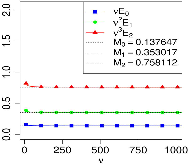
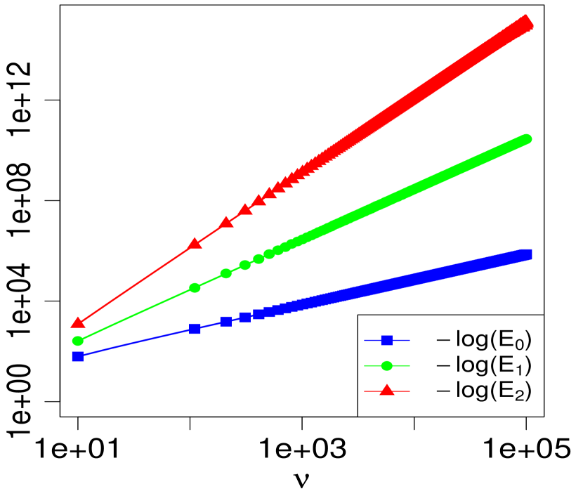
Figure 1: Numerical illustration of the asymptotic constants $M_{i}$ (on the left) and the log-log plot for the maximum absolute errors as a function of $\nu$ (on the right) for the first three levels of approximation.

3 Proofs

Proof of Lemma 1.

By taking the logarithm in (1), we have

$$\log\bigg{(}\frac{f_{\nu}(x)}{\frac{1}{\sqrt{\nu/(\nu-2)}}\phi(\delta_{x})}\bigg{)} =-\frac{1}{2}\log\Big{(}\frac{\nu-2}{2}\Big{)}-\frac{\nu+1}{2}\log\bigg{(}1+\Big{(}\frac{\delta_{x}}{\sqrt{\nu-2}}\Big{)}^{2}\bigg{)}$$ (16)

$$\quad+\log\Gamma\Big{(}\frac{\nu+1}{2}\Big{)}-\log\Gamma\Big{(}\frac{\nu}{2}\Big{)}+\frac{1}{2}\delta_{x}^{2}.$$

Using the expansions

$$\log\Gamma\Big{(}\frac{\nu+1}{2}\Big{)} =\Big{(}\frac{\nu}{2}\Big{)}\log\Big{(}\frac{\nu+1}{2}\Big{)}-\frac{\nu}{2}-\frac{1}{2}+\frac{1}{2}\log(2\pi)$$ (17)

$$\quad+\frac{2}{12(\nu+1)}-\frac{2^{3}}{360(\nu+1)^{3}}+\mathcal{O}(\nu^{-4}),$$

$$\log\Gamma\Big{(}\frac{\nu}{2}\Big{)} =\Big{(}\frac{\nu}{2}-\frac{1}{2}\Big{)}\log\Big{(}\frac{\nu}{2}\Big{)}-\frac{\nu}{2}+\frac{1}{2}\log(2\pi)$$

$$\quad+\frac{2}{12\nu}-\frac{2^{3}}{360\nu^{3}}+\mathcal{O}(\nu^{-5}),$$

(see, e.g., (Abramowitz & Stegun,, 1964, p.257)) and

$$\log\Gamma\Big{(}\frac{\nu+1}{2}\Big{)}-\log\Gamma\Big{(}\frac{\nu}{2}\Big{)} =\Big{(}\frac{\nu}{2}\Big{)}\log\Big{(}\frac{\nu+1}{2}\Big{)}-\Big{(}\frac{\nu}{2}-\frac{1}{2}\Big{)}\log\Big{(}\frac{\nu}{2}\Big{)}$$ (18)

$$\quad-\frac{1}{2}+\frac{2}{12(\nu+1)}-\frac{2}{12\nu}+\mathcal{O}(\nu^{-4})$$

$$=\frac{1}{2}\log\Big{(}\frac{\nu}{2}\Big{)}-\frac{1}{4\nu}+\frac{1}{24\nu^{3}}+\mathcal{O}(\nu^{-4}),$$

we can rewrite (16) as

$$\log\bigg{(}\frac{f_{\nu}(x)}{\frac{1}{\sqrt{\nu/(\nu-2)}}\phi(\delta_{x})}\bigg{)} =-\frac{1}{2}\log\Big{(}\frac{\nu-2}{2}\Big{)}-\frac{\nu+1}{2}\log\bigg{(}1+\Big{(}\frac{\delta_{x}}{\sqrt{\nu-2}}\Big{)}^{2}\bigg{)}$$ (19)

$$\quad+\frac{1}{2}\log\Big{(}\frac{\nu}{2}\Big{)}-\frac{1}{4\nu}+\frac{1}{24\nu^{3}}+\frac{1}{2}\delta_{x}^{2}+\mathcal{O}(\nu^{-4}).$$

Using the Taylor expansions

$$-\frac{1}{2}\log\Big{(}\frac{\nu-2}{2}\Big{)}+\frac{1}{2}\log\Big{(}\frac{\nu}{2}\Big{)}=\frac{1}{\nu}+\frac{1}{\nu^{2}}+\frac{4}{3\nu^{3}}+\mathcal{O}(\nu^{-4}),$$ (20)

and

$$\log(1+y)=y-\frac{y^{2}}{2}+\frac{y^{3}}{3}-\frac{y^{4}}{4}+\mathcal{O}_{\eta}(y^{5}),\quad|y|\leq\eta,$$ (21)

we have

$$\log\bigg{(}\frac{f_{\nu}(x)}{\frac{1}{\sqrt{\nu/(\nu-2)}}\phi(\delta_{x})}\bigg{)} =\frac{3}{4\nu}+\frac{1}{\nu^{2}}+\frac{11}{8\nu^{3}}+\left[\frac{1}{2}-\frac{\nu+1}{2(\nu-2)}\right]\delta_{x}^{2}$$ (22)

$$\quad+\frac{\nu+1}{4(\nu-2)^{2}}\delta_{x}^{4}-\frac{\nu+1}{6(\nu-2)^{3}}\delta_{x}^{6}+\frac{\nu+1}{8(\nu-2)^{4}}\delta_{x}^{8}$$

$$\quad+\mathcal{O}_{\eta}\bigg{(}\frac{1+|\delta_{x}|^{10}}{\nu^{4}}\bigg{)}.$$

Now,

$$\frac{1}{2}-\frac{\nu+1}{2(\nu-2)} =-\frac{3}{2\nu}-\frac{3}{\nu^{2}}-\frac{6}{\nu^{3}}+\mathcal{O}(\nu^{-4}),$$ (23)

$$\frac{\nu+1}{4(\nu-2)^{2}} =\frac{1}{4\nu}+\frac{5}{4\nu^{2}}+\frac{4}{\nu^{3}}+\mathcal{O}(\nu^{-4}),$$

$$-\frac{\nu+1}{6(\nu-2)^{3}} =-\frac{1}{6\nu^{2}}-\frac{7}{6\nu^{3}}+\mathcal{O}(\nu^{-4}),$$

$$\frac{\nu+1}{8(\nu-2)^{4}} =\frac{1}{8\nu^{3}}+\mathcal{O}(\nu^{-4}),$$

so we can rewrite (22) as

$$\log\bigg{(}\frac{f_{\nu}(x)}{\frac{1}{\sqrt{\nu/(\nu-2)}}\phi(\delta_{x})}\bigg{)} =\frac{\frac{1}{4}\delta_{x}^{4}-\frac{3}{2}\delta_{x}^{2}+\frac{3}{4}}{\nu}+\frac{-\frac{1}{6}\delta_{x}^{6}+\frac{5}{4}\delta_{x}^{4}-3\delta_{x}^{2}+1}{\nu^{2}}$$ (24)

$$\quad+\frac{\frac{1}{8}\delta_{x}^{8}-\frac{7}{6}\delta_{x}^{6}+4\delta_{x}^{4}-6\delta_{x}^{2}+\frac{11}{8}}{\nu^{3}}+\mathcal{O}_{\eta}\bigg{(}\frac{1+|\delta_{x}|^{10}}{\nu^{4}}\bigg{)},$$

which proves (7). To obtain (8) and conclude the proof, we take the exponential on both sides of the last equation and we expand the right-hand side with

$$e^{y}=1+y+\frac{y^{2}}{2}+\frac{y^{3}}{6}+\mathcal{O}(e^{\widetilde{\eta}}y^{4}),\quad\text{for }-\infty<y\leq\widetilde{\eta}.$$ (25)

For $\nu$ large enough and uniformly for $x\in B_{\nu}(\eta)$, the right-hand side of (24) is $\mathcal{O}(1)$. When this bound is taken as $y$ in (25), it explains the error in (8). ∎

Proof of Theorem 1.

By large deviation bounds, the approximations are trivial when $a\not\in B_{\nu}(1/2)$. Therefore, for the remainder of the proof, we assume that $a\in B_{\nu}(1/2)$. Let

$$c=\frac{d_{1}}{\nu}+\frac{d_{2}}{\nu^{2}}+\frac{d_{3}}{\nu^{3}},$$ (26)

where $d_{1},d_{2},d_{3}\in\mathbb{R}$ are to be chosen later, then we have the Taylor expansion

$$\int_{\delta_{a-c}}^{\delta_{a}}\phi(y){\rm d}y =\phi(\delta_{a})\int_{\delta_{a-c}}^{\delta_{a}}{\rm d}y+\phi^{\prime}(\delta_{a})\int_{\delta_{a-c}}^{\delta_{a}}(y-\delta_{a}){\rm d}y+\frac{\phi^{\prime\prime}(\delta_{a})}{2}\int_{\delta_{a-c}}^{\delta_{a}}(y-\delta_{a})^{2}{\rm d}y$$ (27)

$$\quad+\mathcal{O}\left(\frac{\phi^{\prime\prime\prime}(\delta_{a})}{6}\int_{\delta_{a-c}}^{\delta_{a}}(y-\delta_{a})^{3}{\rm d}y\right)$$

$$=\phi(\delta_{a})\,\left\{\begin{array}[]{l}\frac{c}{\sqrt{\nu/(\nu-2)}}+\frac{c^{2}\,\delta_{a}}{2\nu/(\nu-2)}+\frac{c^{3}(\delta_{a}^{2}-1)}{6\,\nu^{3/2}/(\nu-2)^{3/2}}+\mathcal{O}\big{(}\frac{1+|\delta_{a}|^{3}}{\nu^{4}}\big{)}\end{array}\right\}$$

$$=\phi(\delta_{a})\,\left\{\begin{array}[]{l}\nu^{-1}\,d_{1}+\nu^{-2}\,\big{(}\frac{\delta_{a}}{2}d_{1}^{2}-d_{1}+d_{2}\big{)}\\[4.2679pt] +\nu^{-3}\,\left(\begin{array}[]{l}\frac{1}{6}(\delta_{a}^{2}-1)d_{1}^{3}-\delta_{a}d_{1}^{2}-\frac{1}{2}d_{1}\\[0.0pt] +\delta_{a}d_{1}d_{2}-d_{2}+d_{3}\end{array}\right)+\mathcal{O}\big{(}\frac{1+|\delta_{a}|^{3}}{\nu^{4}}\big{)}\end{array}\right\}.$$

We also have the straightforward large deviation bounds

$$\int_{[a,\infty)\cap B_{\nu}^{c}(1/2)}f_{\nu}(x){\rm d}x=\mathcal{O}(e^{-\beta\nu^{1/2}}),$$ (28)

$$\int_{[a,\infty)\cap B_{\nu}^{c}(1/2)}\phi(y){\rm d}y=\mathcal{O}(e^{-\beta\nu^{1/2}}),$$

where $\beta>0$ is a small enough constant, and the local approximation in Lemma 1 yields

$$\int_{a}^{\infty}f_{\nu}(x){\rm d}x-\int_{\delta_{a}}^{\infty}\phi(y){\rm d}y =\nu^{-1}\bigg{\{}\frac{1}{4}\Psi_{4}(\delta_{x})-\frac{3}{2}\Psi_{2}(\delta_{x})+\frac{3}{4}\Psi(\delta_{x})\bigg{\}}$$ (29)

$$\quad+\nu^{-2}\left\{\begin{array}[]{l}\frac{1}{32}\Psi_{8}(\delta_{x})-\frac{13}{24}\Psi_{6}(\delta_{x})+\frac{41}{16}\Psi_{4}(\delta_{x})\\[4.2679pt] -\frac{33}{8}\Psi_{2}(\delta_{x})+\frac{41}{32}\Psi(\delta_{x})\end{array}\right\}$$

$$\quad+\nu^{-3}\left\{\begin{array}[]{l}\frac{1}{384}\Psi_{12}(\delta_{x})-\frac{17}{192}\Psi_{10}(\delta_{x})+\frac{127}{128}\Psi_{8}(\delta_{x})\\[4.2679pt] -\frac{457}{96}\Psi_{6}(\delta_{x})+\frac{1357}{128}\Psi_{4}(\delta_{x})\\[4.2679pt] -\frac{651}{64}\Psi_{2}(\delta_{x})+\frac{281}{128}\Psi(\delta_{x})\end{array}\right\}$$

$$\quad+\mathcal{O}(\nu^{-4}),$$

where $\Psi_{k}(\delta_{a})\vcentcolon=\int_{\delta_{a}}y^{k}\phi(y){\rm d}y$. Now, using the fact that

$$\Psi_{12}(\delta_{a})=(10395\delta_{a}+3465\delta_{a}^{3}+693\delta_{a}^{5}+99\delta_{a}^{7}+11\delta_{a}^{9}+\delta_{a}^{11})\phi(\delta_{a})+10395\Psi(\delta_{a}),$$ (30)

$$\Psi_{10}(\delta_{a})=(945\delta_{a}+315\delta_{a}^{3}+63\delta_{a}^{5}+9\delta_{a}^{7}+\delta_{a}^{9})\phi(\delta_{a})+945\Psi(\delta_{a}),$$

$$\Psi_{8}(\delta_{a})=(105\delta_{a}+35\delta_{a}^{3}+7\delta_{a}^{5}+\delta_{a}^{7})\phi(\delta_{a})+105\Psi(\delta_{a}),$$

$$\Psi_{6}(\delta_{a})=(15\delta_{a}+5\delta_{a}^{3}+\delta_{a}^{5})\phi(\delta_{a})+15\Psi(\delta_{a}),$$

$$\Psi_{4}(\delta_{a})=(3\delta_{a}+\delta_{a}^{3})\phi(\delta_{a})+3\Psi(\delta_{a}),$$

$$\Psi_{2}(\delta_{a})=\delta_{a}\phi(\delta_{a})+\Psi(\delta_{a}),$$

where $\Psi$ denotes the survival function of the standard normal distribution, Equations (27), (28) and (29) together yield

$$\int_{a}^{\infty}f_{\nu}(x){\rm d}x-\int_{\delta_{a-c}}^{\infty}\phi(y){\rm d}y$$ (31)

$$\quad=\nu^{-1}\bigg{\{}\frac{1}{4}\delta_{a}^{3}-\frac{3}{4}\delta_{a}-d_{1}\bigg{\}}\phi(\delta_{a})+\nu^{-2}\left\{\begin{array}[]{l}\frac{1}{32}\delta_{a}^{7}-\frac{31}{96}\delta_{a}^{5}+\frac{91}{96}\delta_{a}^{3}-\frac{41}{32}\delta_{a}\\[4.2679pt] -\big{(}\frac{\delta_{a}}{2}d_{1}^{2}-d_{1}+d_{2}\big{)}\end{array}\right\}\phi(\delta_{a})$$

$$\quad\quad+\nu^{-3}\left\{\begin{array}[]{l}\frac{1}{384}\delta_{a}^{11}-\frac{23}{384}\delta_{a}^{9}+\frac{29}{64}\delta_{a}^{7}-\frac{305}{192}\delta_{a}^{5}+\frac{1021}{384}\delta_{a}^{3}-\frac{281}{128}\delta_{a}\\[5.69054pt] -\big{(}\frac{1}{6}(\delta_{a}^{2}-1)d_{1}^{3}-\delta_{a}d_{1}^{2}-\frac{1}{2}d_{1}+\delta_{a}d_{1}d_{2}-d_{2}+d_{3}\big{)}\end{array}\right\}\phi(\delta_{a})+\mathcal{O}(\nu^{-4}).$$

If we select $d_{1}=d_{2}=d_{3}=0$, then

$$\max_{a\in\mathbb{R}}\Big{|}\int_{a}^{\infty}f_{\nu}(x){\rm d}x-\int_{\delta_{a-c}}^{\infty}\phi(y){\rm d}y\Big{|}\leq\nu^{-1}\max_{a\in\mathbb{R}}\frac{|\delta_{a}|}{4}|\delta_{a}^{2}-3|\phi(\delta_{a})+\mathcal{O}(\nu^{-2}),$$ (32)

which proves (10). If we select $d_{1}=\frac{\delta_{a}}{4}(\delta_{a}^{2}-3)$ and $d_{2}=d_{3}=0$ to cancel the first brace in (31), then

$$\max_{a\in\mathbb{R}}\Big{|}\int_{a}^{\infty}f_{\nu}(x){\rm d}x-\int_{\delta_{a-c}}^{\infty}\phi(y){\rm d}y\Big{|}$$ (33)

$$\leq\nu^{-2}\max_{a\in\mathbb{R}}\frac{|\delta_{a}|}{96}|13\delta_{a}^{4}-88\delta_{a}^{2}+195|\phi(\delta_{a})+\mathcal{O}(\nu^{-3}),$$

which proves (11). If we select $d_{1}=\frac{\delta_{a}}{4}(\delta_{a}^{2}-3)$, $d_{2}=-\frac{\delta_{a}}{96}(13\delta_{a}^{4}-88\delta_{a}^{2}+195)$ and $d_{3}=0$ to cancel the first two braces in (31), then

$$\max_{a\in\mathbb{R}}\Big{|}\int_{a}^{\infty}f_{\nu}(x){\rm d}x-\int_{\delta_{a-c}}^{\infty}\phi(y){\rm d}y\Big{|}$$ (34)

$$\leq\nu^{-3}\max_{a\in\mathbb{R}}\frac{|\delta_{a}|}{384}|35\delta_{a}^{6}-293\delta_{a}^{4}+1025\delta_{a}^{2}-1767|\phi(\delta_{a})+\mathcal{O}(\nu^{-4}),$$

which proves (12). If we select $d_{1}=\frac{\delta_{a}}{4}(\delta_{a}^{2}-3)$, $d_{2}=-\frac{\delta_{a}}{96}(13\delta_{a}^{4}-88\delta_{a}^{2}+195)$ and $d_{3}=-\frac{\delta_{a}}{384}(35\delta_{a}^{6}-293\delta_{a}^{4}+1025\delta_{a}^{2}-1767)$ to cancel the three braces in (31), then

$$\max_{a\in\mathbb{R}}\Big{|}\int_{a}^{\infty}f_{\nu}(x){\rm d}x-\int_{\delta_{a-c}}^{\infty}\phi(y){\rm d}y\Big{|}=\mathcal{O}(\nu^{-4}),$$ (35)

which proves (13). This ends the proof. ∎

Proof of Theorem 2.

Let $\alpha=S_{\nu}(\lambda)$ for some $\lambda\in B_{\nu}(\eta)$ and $\eta\in(0,1)$. By Theorem 1, we have, as $\nu\to\infty$,

$$\left|\alpha-\Psi(\delta_{\lambda-\sum_{k=1}^{i}d_{k}/\nu^{k}})\right|\leq\frac{C_{i}^{\prime}}{\nu^{i+1}},\quad i\in\{0,1,2,3\},$$ (36)

for some universal constants $C_{i}^{\prime}$. A Taylor expansion for $\Psi$ at $\lambda$ yields, for $x=\lambda+\mathcal{O}(\nu^{-1})$,

$$\frac{\Psi(x)}{\phi(\lambda)}=\frac{\Psi(\lambda)}{\phi(\lambda)}-\sum_{k=1}^{i}\frac{\phi^{(k-1)}(\lambda)}{\phi(\lambda)\,k!}(x-\lambda)^{k}+\mathcal{O}(\nu^{-(i+1)}),\quad i\in\{0,1,2,3\},$$ (37)

namely,

$$\frac{\Psi(x)}{\phi(\lambda)} =\frac{\Psi(\lambda)}{\phi(\lambda)}-(x-\lambda)+\mathcal{O}(\nu^{-2}),\quad\text{for }i=1,$$ (38)

$$\frac{\Psi(x)}{\phi(\lambda)} =\frac{\Psi(\lambda)}{\phi(\lambda)}-(x-\lambda)+\frac{\lambda}{2}(x-\lambda)^{2}+\mathcal{O}(\nu^{-3}),\quad\text{for }i=2,$$

$$\frac{\Psi(x)}{\phi(\lambda)} =\frac{\Psi(\lambda)}{\phi(\lambda)}-(x-\lambda)+\frac{\lambda}{2}(x-\lambda)^{2}-\frac{(\lambda^{2}-1)}{6}(x-\lambda)^{3}+\mathcal{O}(\nu^{-4}),\quad\text{for }i=3.$$

By applying these formulas with $x=\delta_{\lambda-\sum_{k=1}^{i}d_{k}/\nu^{k}}$, together with the fact that

$$\delta_{\lambda-\sum_{k=1}^{i}d_{k}/\nu^{k}}-\lambda =\sqrt{\frac{\nu-2}{\nu}}\left\{\lambda-\sum_{k=1}^{i}\frac{d_{k}}{\nu^{k}}\right\}-\lambda$$ (39)

$$=-\frac{\lambda}{\nu}-\frac{\lambda}{2\nu^{2}}-\frac{\lambda}{2\nu^{3}}+\mathcal{O}(\nu^{-4})-\left(1-\frac{1}{\nu}-\frac{1}{2\nu^{2}}+\mathcal{O}(\nu^{-3})\right)\sum_{k=1}^{i}\frac{d_{k}}{\nu^{k}},$$

we get

$$\frac{\alpha}{\phi(\lambda)} =\frac{\Psi(\lambda)}{\phi(\lambda)}+\left(\frac{\lambda}{\nu}+\frac{d_{1}}{\nu}\right)+\mathcal{O}(\nu^{-2}),\quad\text{for }i=1,$$ (40)

$$\frac{\alpha}{\phi(\lambda)} =\frac{\Psi(\lambda)}{\phi(\lambda)}+\left(\frac{\lambda}{\nu}+\frac{\lambda}{2\nu^{2}}+\frac{d_{1}}{\nu}+\frac{d_{2}}{\nu^{2}}-\frac{d_{1}}{\nu^{2}}\right)$$

$$\quad+\frac{\lambda}{2}\left(\frac{\lambda^{2}}{\nu^{2}}+\frac{2\lambda d_{1}}{\nu^{2}}+\frac{d_{1}^{2}}{\nu^{2}}\right)+\mathcal{O}(\nu^{-3}),\quad\text{for }i=2,$$

$$\frac{\alpha}{\phi(\lambda)} =\frac{\Psi(\lambda)}{\phi(\lambda)}+\left(\frac{\lambda}{\nu}+\frac{\lambda}{2\nu^{2}}+\frac{\lambda}{2\nu^{3}}+\frac{d_{1}}{\nu}+\frac{d_{2}}{\nu^{2}}+\frac{d_{3}}{\nu^{3}}-\frac{d_{1}}{\nu^{2}}-\frac{d_{2}}{\nu^{3}}-\frac{d_{1}}{2\nu^{3}}\right)$$

$$\quad+\frac{\lambda}{2}\left(\frac{\lambda^{2}}{\nu^{2}}+\frac{2\lambda d_{1}}{\nu^{2}}+\frac{d_{1}^{2}}{\nu^{2}}+\frac{\lambda^{2}}{\nu^{3}}+\frac{2\lambda d_{2}}{\nu^{3}}-\frac{\lambda d^{1}}{\nu^{3}}+\frac{2d_{1}d_{2}}{\nu^{3}}-\frac{2d_{1}^{2}}{\nu^{3}}\right)$$

$$\quad+\frac{(\lambda^{2}-1)}{6}\left(\frac{\lambda^{3}}{\nu^{3}}+\frac{d_{1}^{3}}{\nu^{3}}\right)+\mathcal{O}(\nu^{-4}),\quad\text{for }i=3.$$

This ends the proof. ∎

Funding

F. Ouimet is supported by postdoctoral fellowships from the NSERC (PDF) and the FRQNT (B3X supplement and B3XR).

Conflicts of interest

The author declares no conflict of interest.

References

References

- Abramowitz & Stegun, (1964) Abramowitz, M., & Stegun, I. A. 1964. Handbook of Mathematical Functions with Formulas, Graphs, and Mathematical Tables. National Bureau of Standards Applied Mathematics Series, vol. 55. For sale by the Superintendent of Documents, U.S. Government Printing Office, Washington, D.C.
- Cressie, (1978) Cressie, N. 1978. A finely tuned continuity correction. Ann. Inst. Statist. Math., 30(3), 435–442.
- Esseen, (1945) Esseen, C.-G. 1945. Fourier analysis of distribution functions. A mathematical study of the Laplace-Gaussian law. Acta Math., 77, 1–125.
- Gaunt, (2014) Gaunt, R. E. 2014. Variance-gamma approximation via Stein’s method. Electron. J. Probab., 19, no. 38, 33 pp.
- Gaunt, (2020) Gaunt, R. E. 2020. Wasserstein and Kolmogorov error bounds for variance-gamma approximation via Stein’s method I. J. Theoret. Probab., 33(1), 465–505.
- Gaunt, (2021) Gaunt, R. E. 2021. New error bounds for Laplace approximation via Stein’s method. ESAIM Probab. Stat., 25, 325–345.
- Goldberg & Levine, (1946) Goldberg, H., & Levine, H. 1946. Approximate formulas for the percentage points and normalization of and . Ann. Math. Statistics, 17, 216–225.
- Govindarajulu, (1965) Govindarajulu, Z. 1965. Normal approximations to the classical discrete distributions. Sankhyā Ser. A, 27, 143–172.
- Harley, (1957) Harley, B. I. 1957. Relation between the distributions of non-central and of a transformed correlation coefficient. Biometrika, 44(1-2), 219–224.
- Hendricks, (1936) Hendricks, W. A. 1936. An approximation to “Student’s” distribution. Ann. Math. Statist., 7(4), 210–221.
- Jennett & Welch, (1939) Jennett, W. J., & Welch, B. L. 1939. The control of proportion defective as judged by a single quality characteristic varying on a continuous scale. J. R. Stat. Soc. (Supplement to), 6(1), 80–88.
- Johnson & Welch, (1940) Johnson, N. L., & Welch, B. L. 1940. Applications of the non-central -distribution. Biometrika, 31, 362–389.
- Merrington & Pearson, (1958) Merrington, M., & Pearson, E. S. 1958. An approximation to the distribution of non-central . Biometrika, 45(3/4), 484–491.
- Ouimet, (2021a) Ouimet, F. 2021a. On the Le Cam distance between Poisson and Gaussian experiments and the asymptotic properties of Szasz estimators. J. Math. Anal. Appl., 499(1), Paper No. 125033, 18 pp.
- Ouimet, (2021b) Ouimet, F. 2021b. A precise local limit theorem for the multinomial distribution and some applications. J. Statist. Plann. Inference, 215, 218–233.
- Ouimet, (2021c) Ouimet, F. 2021c. A refined continuity correction for the negative binomial distribution and asymptotics of the median. Preprint, 1–18. arXiv:2103.08846v1.
- Ouimet, (2022a) Ouimet, F. 2022a. An improvement of Tusnády’s inequality in the bulk. Adv. in Appl. Math., 133, Paper No. 102270, 24 pp.
- Ouimet, (2022b) Ouimet, F. 2022b. A multivariate normal approximation for the Dirichlet density and some applications. Stat, 11, Paper No. e410, 13 pp.
- Ouimet, (2022c) Ouimet, F. 2022c. On the Le Cam distance between multivariate hypergeometric and multivariate normal experiments. Results Math., 77(1), Paper No. 47, 11 pp.
- Ouimet, (2022d) Ouimet, F. 2022d. A symmetric matrix-variate normal local approximation for the Wishart distribution and some applications. J. Multivariate Anal., 189, Paper No. 104923, 17 pp.
- Owen, (1958) Owen, D. B. 1958 (4). Tables of factors for one-sided tolerance limits for a normal distribution. Tech. rept. U.S. Department of Energy Office of Scientific and Technical Information.
- Resnikoff & Lieberman, (1957) Resnikoff, G. J., & Lieberman, G. J. 1957. Tables of the Non-Central -Distribution: Density Function, Cumulative Distribution Function and Percentage Points. Stanford Studies in Mathematics and Statistics, I. Stanford University Press, Stanford, California.
- Shafiei & Saberali, (2015) Shafiei, A., & Saberali, S. M. 2015. A simple asymptotic bound on the error of the ordinary normal approximation to the Student’s -distribution. IEEE Commun. Lett., 19(8), 1295–1298.
- van Eeden, (1961) van Eeden, C. 1961. Some approximations to the percentage points of the non-central -distribution. Rev. Inst. Internat. Statist., 29, 4–31.