Quasi-Newton Acceleration of EM and MM Algorithms via Broyden’s Method

Abstract

The principle of majorization-minimization (MM) provides a general framework for eliciting effective algorithms to solve optimization problems. However, they often suffer from slow convergence, especially in large-scale and high-dimensional data settings. This has drawn attention to acceleration schemes designed exclusively for MM algorithms, but many existing designs are either problem-specific or rely on approximations and heuristics loosely inspired by the optimization literature. We propose a novel, rigorous quasi-Newton method for accelerating any valid MM algorithm, cast as seeking a fixed point of the MM algorithm map. The method does not require specific information or computation from the objective function or its gradient, and enjoys a limited-memory variant amenable to efficient computation in high-dimensional settings. By connecting our approach to Broyden’s classical root-finding methods, we establish convergence guarantees and identify conditions for linear and super-linear convergence. These results are validated numerically and compared to peer methods in a thorough empirical study, showing that it achieves state-of-the-art performance across a diverse range of problems.

1 Introduction

Iterative procedures are becoming increasingly prevalent for statistical tasks that are cast as optimization of an objective function (Everitt,, 2012). The canonical setting of minimizing a measure of fit together with a penalty term sits at the heart of statistics, yet challenges still arise from high dimensionality, missing data, constraints, and other aspects of contemporary data. The principle of majorization-minimization (MM) provides a framework for designing effective algorithms well-suited for such problems lacking a closed form solution. Perhaps the most well-known special case is the expectation-maximization (EM) algorithm, a workhorse for maximum likelihood estimation under missing data. Besides EM, instances of MM abound in statistics, ranging from matrix factorization (Lee and Seung,, 1999) to nonconcave penalized likelihood estimation (Zou and Li,, 2008). The MM principle is attractive because it admits algorithms that (1) are simple to implement and (2) provide stable performance by obeying monotonicity in the objective (Dempster et al.,, 1977; Laird,, 1978).

Consider $\boldsymbol{x}\in\mathbb{R}^{p}$ and the goal of minimizing a “difficult” objective function $f\mathrel{\mathop{\mathchar 58\relax}}\mathbb{R}^{p}\to\mathbb{R}$, i.e. finding $\displaystyle\boldsymbol{x}^{\ast}=\text{argmin}_{\boldsymbol{x}}f(\boldsymbol{x})$, which is not available in closed form. An MM algorithm transfers this task onto an iterative scheme, successively minimizing a sequence of surrogate functions which dominate the objective function $f$ and are tangent to it at the current iterate $\boldsymbol{x}_{k}$. This renders an MM algorithm map $F$, updating $\boldsymbol{x}_{k}$ to $\boldsymbol{x}_{k+1}=F(\boldsymbol{x}_{k})$.

However, MM algorithms typically converge at a locally linear rate, which can translate to impractically slow progress in many statistical problems, especially in high dimensions (Wu,, 1983; Boyles,, 1983; Meng and Rubin,, 1994). To address this issue, a body of work designs general acceleration schemes for numerical optimization methods including Nesterov’s schemes (Nesterov,, 1983), SAG (Schmidt et al.,, 2017), SAGA (Defazio et al.,, 2014), catalyst acceleration (Lin et al.,, 2017), and SDCA (Shalev-Shwartz and Zhang,, 2014). Special attention has also been given towards acceleration methods specifically designed for MM algorithms (Jamshidian and Jennrich,, 1997, 1993; Lange,, 1995; Zhou et al.,, 2011). Broadly, these methods seek additional information to better inform the search direction and/or step lengths of the unadorned algorithm. Improvements may come from high order differentials of the objective or MM algorithm map that incur additional computational cost. As a result, it becomes necessary to balance these tradeoffs.

One approach employs hybrid accelerators (Jamshidian and Jennrich,, 1997) rely on working directly on the original objective function $f$ (Lange,, 1995; Jamshidian and Jennrich,, 1997, 1993), often requiring second order derivatives denoted by $d^{2}f$. Approximations to $d^{2}f$ can then be obtained via Fisher scoring in the case of EM. Outside of the context of missing data, classical tools such as quasi-Newton and conjugate gradient methods can be applied to the objective to similar effect. However, an advantage of MM algorithms lies in sidestepping unwieldy objectives in favor of operating on simpler surrogates—for instance, EM works well because it bypasses the need to consider the observed data log-likelihood. Therefore, hybrid methods unfortunately fail to preserve this key advantage of MM algorithms.

An alternative is to instead consider accelerating the MM algorithm map $F$ directly in a way that is largely agnostic to the optimization objective. These have been classified as pure accelerators; see Jamshidian and Jennrich, (1997). One class of pure first-order accelerators is given by quasi-Newton (QN) algorithms, which utilize an approximate Jacobian of $F$, denoted by $dF$, to find a fixed point $\boldsymbol{x}^{*}$ such that $F(\boldsymbol{x}^{*})=\boldsymbol{x}^{*}$. Equivalently, the goal is to find the root of the MM residual $G(\boldsymbol{x})\mathrel{\mathop{\mathchar 58\relax}}=F(\boldsymbol{x})-\boldsymbol{x}$. Jamshidian and Jennrich, (1997) explicitly apply Broyden’s classical root-finding algorithm (Broyden,, 1965) for this purpose. As we outlay our method, we will demonstrate that further improvement can be achieved by modifying a general Broyden-type method (Broyden et al.,, 1973) that leverages extra information from the MM map. The STEM and SQUAREM methods of Varadhan and Roland, (2008) approximate this Jacobian by a scalar multiple of the identity matrix. The QN method of Zhou et al., (2011) proposes a computationally elegant approximation derived from an assumption of nearness to the stationary point. These pure accelerators tend to preserve the simplicity, convergence properties, and low computational cost of the original algorithm. However, they often rely on heuristic approximations of $dG$ (or $dG^{-1}$), or derivations that potentially ignore a large amount of crucial first-order information. While loosely inspired by the theory behind classical quasi-Newton methods, it can be argued that these methods do not fully and formally take advantage of the prior optimization literature.

This paper seeks to fill the methodological gap by proposing a generic accelerator for any MM algorithm map via a quasi-Newton root-finding method. Casting the problem as root-finding leads to robustness against numerical instabilities. We build off of the wisdom in Zhou et al., (2011), referring to their method as ZAL in this paper, and a few other methods (briefly discussed in Section 2) that also seek to find the root of MM residuals using QN method. Various QN methods differ from one another in the way $dG(\boldsymbol{x})^{-1}$ is approximated. Popular methods model this approximation as solution to constrained optimization problem where the linear constraints are provided by secant approximation of $G$. Our method incorporates the information from the MM algorithm map to better inform the secant approximation. While ZAL minimizes the norm of the Jacobian near the fixed point, we optimize a richer objective that directly ties into the classical approach of minimizing the change in the Jacobian across iterations, furnishing a rank-two update formula for $dG^{-1}$. This simple yet effective approach guarantees MM acceleration in a more generalized setting and allows us to establish theoretical convergence guarantees.

This paper is organised as follows: in Section 2, we present a general background of MM algorithms and existing acceleration techniques. The key contribution of this paper is formally proposing the MM acceleration algorithm and writing its proof of convergence in Section 3. Our standard quasi-Newton recipe demands storing the approximate Jacobian matrices in each iteration, which can be computationally ineffective for high dimensions. To address this issue, we further propose a limited-memory variant of our method amenable to high-dimensional settings. We then assess the performance of our algorithm empirically in Section 4, followed by discussion.

2 Background: EM, MM, and Acceleration

MM algorithms are increasingly popular toward solving large-scale and high-dimensional optimization problems in statistics and machine learning (Lange and Wu,, 2008; Zhou et al.,, 2015; Xu and Lange,, 2019). An MM algorithm minimizes the objective function $f$ by successively minimizing a sequence of surrogate functions $g(\boldsymbol{x}\mid\boldsymbol{x}_{k})$ which dominate the objective function $f(\boldsymbol{x})$ and are tangent to it at the current iterate $\boldsymbol{x}_{k}$. That is, they require that $g(\boldsymbol{x}_{k}\mid\boldsymbol{x}_{k})=f(\boldsymbol{x}_{k})$ and $g(\boldsymbol{x}\mid\boldsymbol{x}_{k})\geq f(\boldsymbol{x})$ for all $\boldsymbol{x}$ at each iteration $k$. Decreasing $g(\boldsymbol{x}\mid\boldsymbol{x}_{k})$ automatically engenders a decrease in $f(\boldsymbol{x})$. The resulting update $\boldsymbol{x}_{k+1}~{}=~{}\text{argmin}_{\boldsymbol{x}}g(\boldsymbol{x}\mid\boldsymbol{x}_{k})$ implies the string of inequalities $f(\boldsymbol{x}_{k+1})\leq g(\boldsymbol{x}_{k+1}\mid\boldsymbol{x}_{k})\leq g(\boldsymbol{x}_{k}\mid\boldsymbol{x}_{k})=f(\boldsymbol{x}_{k})$ validating the descent property. Our method will make use of this practically useful observation. The MM principle thus converts a hard optimization problem into a sequence of manageable subproblems, expressed as $\boldsymbol{x}_{k+1}=F(\boldsymbol{x}_{k})$.

The iteration terminates when a chosen vector norm (usually $L_{2}$ norm) of differences between two consecutive iterates is small enough, i.e. $\|\Delta\boldsymbol{x}_{k}\|=\|\boldsymbol{x}_{k+1}-\boldsymbol{x}_{k}\|\leq\epsilon$ for some tolerance $\epsilon>0$. From the perspective of the algorithm map, the MM algorithm amounts to seeking the root of $G(\boldsymbol{x})\mathrel{\mathop{\mathchar 58\relax}}=F(\boldsymbol{x})-\boldsymbol{x}$. This approach has paved the way for QN acceleration regimes that attempt to well-approximate the inverse of the Jacobian of $G$ at $\boldsymbol{x}_{k}$; see Luenberger et al., (1984); Dennis Jr and Schnabel, (1996) for a more detailed discussion. Let $dG(\boldsymbol{x})$ be the differential of $G$ evaluated at $\boldsymbol{x}$, then $dG(\boldsymbol{x})=(dF(\boldsymbol{x})-I_{p})$ where $I_{p}$ is the $p\times p$ identity matrix. Denoting the approximation to $dG(\boldsymbol{x}_{k})^{-1}$ by $H_{k}$, the QN update of $\boldsymbol{x}_{k}$ is given by

$$\boldsymbol{x}_{k+1}=\boldsymbol{x}_{k}-H_{k}G(\boldsymbol{x}_{k})\,.$$ (1)

A QN method is uniquely defined by the way it approximates $dG(\boldsymbol{x}_{k})^{-1}$. The thread tying different QN methods is the secant condition, which states that $H_{k}$ is the exact inverse Jacobian of a linear function joining $(\boldsymbol{x}_{k},G(\boldsymbol{x}_{k}))$ and some other point of choice, say $(\boldsymbol{y},G(\boldsymbol{y}))$. That is, the secant constraint mandates that $H_{k}$ satisfies

$$\boldsymbol{x}_{k}-\boldsymbol{y}=H_{k}(G(\boldsymbol{x}_{k})-G(\boldsymbol{y}))\,.$$ (2)

In the classical Broyden method, $\boldsymbol{y}$ is taken to be $\boldsymbol{x}_{k-1}$. For $\boldsymbol{x}\in\mathbb{R}^{p}$, $H_{k}$ is a $p\times p$ matrix and the secant constraint fixes $p$ degrees of freedom. The remaining $p^{2}-p$ degrees entail that Eq.(2) is underdetermined, satisfied by infinitely many solutions $H_{k}$. At this juncture, deriving QN methods proceeds by specifying an additional criterion to admit a well-defined procedure. We now survey various popular approaches along this line of thought.

2.1 Existing MM Acceleration Schemes

Perhaps the most transparent and well-studied QN acceleration scheme was proposed by Jamshidian and Jennrich, (1997). Their method directly applies the QN method for root finding by Broyden, (1965) to update $H_{k}$ at any time point $k$. Contributions since have noted that this dense matrix update becomes computationally prohibitive in high dimensions typical of contemporary data. The STEM method by Varadhan and Roland, (2008) instead provides a simpler approximation of $H_{k}$ as only a scalar multiple of the identity matrix. Assuming $H_{k}=\alpha_{k}I_{p}$, three variants of STEM entail slightly different inverse Jacobian approximations under

$$\alpha_{k}^{(1)}=\dfrac{\boldsymbol{u}_{k}^{T}\boldsymbol{v}_{k}}{\boldsymbol{v}_{k}^{T}\boldsymbol{v}_{k}},\qquad\qquad\alpha_{k}^{(2)}=\dfrac{\boldsymbol{u}_{k}^{T}\boldsymbol{u}_{k}}{\boldsymbol{u}_{k}^{T}\boldsymbol{v}_{k}},\qquad\qquad\alpha_{k}^{(3)}=-\dfrac{\|\boldsymbol{u}_{k}\|}{\|\boldsymbol{v}_{k}\|}\,,$$ (3)

where

$$\boldsymbol{u}_{k}=F(\boldsymbol{x}_{k})-\boldsymbol{x}_{k},\quad\text{and}\quad\boldsymbol{v}_{k}\,=\,G(F(\boldsymbol{x}_{k}))-G(\boldsymbol{x}_{k})\,=\,F^{2}(\boldsymbol{x}_{k})-2F(\boldsymbol{x}_{k})+\boldsymbol{x}_{k}.$$

The scalars $\alpha_{k}$ in (3) can be understood as various steplengths for each update rule. An extension to STEM known as SQUAREM was later proposed by the same authors (Varadhan and Roland,, 2008), using the idea of a “squared” Cauchy method which may outperform traditional Cauchy methods. While SQUAREM outperforms many acceleration methods and is chiefly regarded for its simplicity, the loss of information due to the identity matrix approximation can remain severe, especially in high dimensional cases.

More recently, Zhou et al., (2011) propose an effective acceleration scheme which we will refer to as ZAL. It enjoys the same computational complexity as SQUAREM by avoiding matrix approximation of $dG(\boldsymbol{x}_{k})^{-1}$ in Eq.(1) at each step, with update rule

$$\boldsymbol{x}_{k+1}=\boldsymbol{x}_{k}-\left(I_{p}-\dfrac{\boldsymbol{v}_{k}\boldsymbol{u}_{k}^{T}}{\boldsymbol{u}_{k}^{T}\boldsymbol{u}_{k}}\right)^{-1}G(\boldsymbol{x}_{k})=(1-c_{k})F(\boldsymbol{x}_{k})+c_{k}F^{2}(\boldsymbol{x}_{k})$$

where $c_{k}=\boldsymbol{u}_{k}^{T}\boldsymbol{u}_{k}/\boldsymbol{u}_{k}^{T}\boldsymbol{v}_{k}$ and the differences $\boldsymbol{u}_{k},\boldsymbol{v}_{k}$ are as defined earlier. It is worth mentioning the secant constraint used in ZAL, as we will motivate a similar constraint to define the endpoints for our method in the next section. Let $M\mathrel{\mathop{\mathchar 58\relax}}=dF(\boldsymbol{x}^{\ast})$. ZAL assumes that $\boldsymbol{x}_{k}$ is close to the optimal point $\boldsymbol{x}^{\ast}$ so that the following linear approximation is reasonable:

$$F\circ F(\boldsymbol{x}_{k})-F(\boldsymbol{x}_{k})\approx M(F(\boldsymbol{x}_{k})-\boldsymbol{x}_{k})\,.$$ (4)

At each step, ZAL attempts to better approximate $M$ using new information from QN updates in the iteration defined by Eq. (1). As these methods operate only with reference to the algorithm map, largely ignoring the objective function to be minimized, they will serve as comparisons for our proposed method. In the following section, we begin by presenting our secant approximation and examine its merits within Broyden’s quasi-Newton paradigm on a univariate illustrative example.

3 A novel Broyden quasi-Newton method

Recall the QN secant approximation given in Equation (2). Motivated by Zhou et al., (2011), using the MM update $F(\boldsymbol{x}_{k})$ as our choice of $\boldsymbol{y}$ gives the following secant constraint

$$F(\boldsymbol{x}_{k})-\boldsymbol{x}_{k}=H_{k}(G(F(\boldsymbol{x}_{k}))-G(\boldsymbol{x}_{k}))\,.$$ (5)

This serves as our point of departure for deriving our proposed method. Before presenting the details, we begin with an illustrative example that highlights the contrast between the secant condition (5) and Broyden’s standard method.

Illustrative Example.

We begin by accelerating a classic MM example of minimizing the cosine function $f(x)=\cos(x)$ to find the root of MM residual. To derive a surrogate, consider the following quadratic expansion about $y\in\mathbb{R}$:

$$\cos(x)\, =\,\cos(y)-\sin(y)(x-y)-\frac{1}{2}\cos(z)(x-y)^{2}$$

$$\,\leq\cos(y)-\sin(y)(x-y)+\frac{1}{2}(x-y)^{2}\,\,\mathrel{\mathop{\mathchar 58\relax}}=\,\,g(x\mid y),$$

where $z$ lies between $x,y$ and the inequality follows since $|\cos(z)|\leq 1$ (Lange,, 2016). It is straightforward to minimize $g$ and obtain the nonlinear MM update formula $x_{k+1}=F(x_{k})=x_{k}+\sin(x_{k})\,$ where the interest is in finding the root of $G(x)\,=\,F(x)-x\,=\,\sin(x)$.

Figure 1 presents two consecutive steps of the QN method for finding root of $G$ in one scenario after two initial iterations labeled $A$ and $B$.. Each plot shows the updates resulting from both secant approximations. We use capital letters to denote a point on the Cartesian plane, and lowercase to denote its corresponding $x$-coordinate. In the left figure, note $a$ and $b$ lie on opposite sides of the root $x^{\ast}=\pi$, marked by the vertical dashed line.

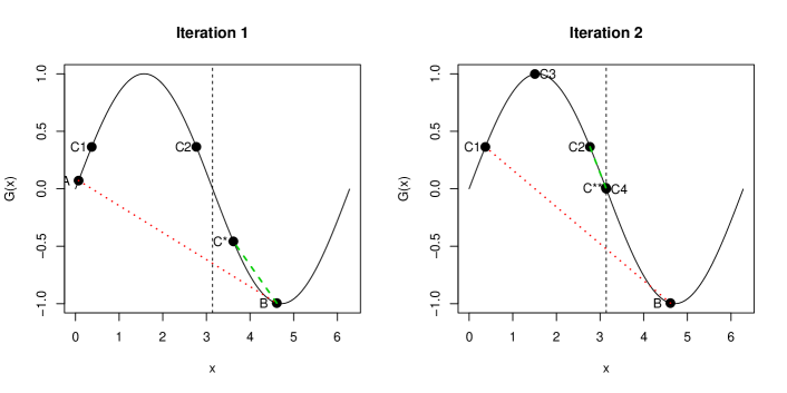
Figure 1: Comparison of secant approximations for two consecutive iterations.

Now let $c^{\ast}=F(b)$ be the unaccelerated MM update from $b$. Rather than moving to $C^{\ast}$, the standard Broyden iteration approximates the search direction as the slope of the line joining A and B (dotted red line). Instead, our proposed update derived in the next section employs the line joining $B$ and $C^{*}$ as the search direction (dashed green line). As a result, Broyden’s method produces $C_{1}$ as the next iterate, and our modified update leads to $C_{2}$. Specifically, the updates are given by

$$c_{1}=b-G(b)\dfrac{b-a}{G(b)-G(a)}\qquad\text{and}\qquad c_{2}=b-G(b)\dfrac{c^{*}-b}{G(c^{*})-G(b)}\,.$$

The difference in quality of the approximations is revealed upon considering the next step as displayed in the right panel. Let $c^{**}=F(c_{2})$, and denote the updates given by standard Broyden’s method and our method as $C_{3}$ and $C_{4}$, respectively. Not only is it visually evident that standard Broyden iteration is far from the optimum, but our modified Broyden with extrapolation method converges at $C_{4}$ under an absolute tolerance criterion of $10^{-7}$.

Even in a univariate setting, where $H_{k}$ can be completely determined from the secant condition, the advantage provided by our secant approximation is clear when the current state does not render a good search direction. Because the secants drawn in standard Broyden’s method rely only linearly on the current and previous state, a bad quasi-Newton step propagates to a bad secant approximation, straying far from the fixed point. Our proposed method avoids this by drawing a secant that incorporates information at the current state together with an extrapolation from the next MM step. This additional information can act as a correction when the original algorithm produces a poor update such as $b$ in the example above.

Method	Minimum	I Quantile	II Quantile	III Quantile	Maximum
QN	2	4	5	6	1389
BQN	1	2	3	3	10

Table 1: Summary of number of iterations until convergence for both methods

To showcase the advantage in the illustrative example over a large range of starting points, we run the two QN methods for $1000$ replications, starting from randomly generated points between $0$ and $2\pi$. Table 1 gives the summary of the number of iterations until convergence for both methods.

While this example would have been trivial to optimize directly, it illustrates an advantage that tends to become more pronounced in higher dimensions where the added directional information we harness from the MM extrapolation is richer. Next, we derive our QN acceleration method using the general form of this secant approximation where $p\geq 2$.

Deriving the proposed method.

Recall that we are interested in finding the root of $G(\boldsymbol{x})$ numerically using QN method. Using the differences $\boldsymbol{u}_{k},\boldsymbol{v}_{k}$ as introduced in the previous section, the secant condition in Eq.(5) can be expressed as $H_{k}\boldsymbol{v}_{k}=\boldsymbol{u}_{k}$. Note that one may impose several secant approximations $H_{k}(\boldsymbol{v}_{k}^{i})=\boldsymbol{u}_{k}^{i}$ for $i\in\{1,...,q\}$ for any $q<p$. These can be generated at the current iterate $\boldsymbol{x}_{k}$ and previous $(q-1)$ iterates, and may yield better performance at the cost of extra computation. To this end, let $U_{k}=(\boldsymbol{u}_{1}\ \dots\boldsymbol{u}_{q})$ and $V_{k}=(\boldsymbol{v}_{1}\;\boldsymbol{v}_{2}\dots\boldsymbol{v}_{q})$ be two $\ p\times q$ matrices; the corresponding linear constraint for $H_{k}$ in the multiple secant conditions case is $H_{k}V_{k}=U_{k}$.

The $p\times p$ inverse Jacobian matrix $H_{k}$ has $p^{2}$ degrees of freedom, of which $pq$ degrees of freedom are fixed by the secant approximation. To derive a well-defined update, one must choose how to fix the remaining $p^{2}-pq$ degrees of freedom. We follow classical intuitions that yield a connection to Broyden’s method for finding roots of nonlinear functions. The idea behind this and several of the most successful quasi-Newton methods seeks the smallest perturbation to $H_{k-1}$ when updating to $H_{k}$, which can also be viewed as imposing a degree of smoothness in the sequence of iterates. The resulting optimization problem can be formulated as

Minimize $$\mathrel{\mathop{\mathchar 58\relax}}\|H_{k}-H_{k-1}\|_{F}\,$$

subject to $$\mathrel{\mathop{\mathchar 58\relax}}H_{k}V_{k}=U_{k}\;,$$ (6)

where $\|\cdot\|_{F}$ denotes the Frobenius norm. We now take partial derivatives of the Lagrangian

$$\mathcal{L}=\dfrac{1}{2}\|H_{k}-H_{k-1}\|^{2}_{F}+\Lambda^{T}(H_{k}V_{k}-U_{k})$$

with respect to $h_{k}^{ij}$ and set to ${0}$. Here $h_{k}^{ij}$ denotes the $ij^{th}$ element of the matrix $H_{k}$. As a consequence, we obtain the Lagrange multiplier equation

$$0=h_{k}^{ij}-h_{k-1}^{ij}+\sum_{k=1}^{p}\lambda_{ik}v_{jk},$$

which can be expressed in matrix form as

$$H_{k}-H_{k-1}+\Lambda V_{k}^{T}=\mathbf{0}.$$ (7)

Right-multiplying Eq.(7) by $V_{k}$ and imposing the constraint from Eq.(5) gives the solution for $\Lambda$ as

$$\Lambda=(H_{k-1}V_{k}-U_{k})(V_{k}^{T}V_{k})^{-1}\,.$$

Therefore,

$$H_{k}=H_{k-1}\left(I_{p}-V_{k}(V_{k}^{T}V_{k})^{-1}V_{k}^{T}\right)+U_{k}(V_{k}^{T}V_{k})^{-1}V_{k}^{T}.$$ (8)

We remark that as the problem dimension increases, a larger choice of $q$ fixes more information and may improve acceleration, but also risks numerical singularity for the matrix $V_{k}^{T}V_{k}$. We draw attention to the special case of $q=1$ where

$$H_{k}=H_{k-1}-H_{k-1}\dfrac{\boldsymbol{v}_{k}\boldsymbol{v}_{k}^{T}}{\boldsymbol{v}_{k}^{T}\boldsymbol{v}_{k}}+\dfrac{\boldsymbol{u}_{k}\boldsymbol{v}_{k}^{T}}{\boldsymbol{v}_{k}^{T}\boldsymbol{v}_{k}}\,.$$ (9)

We see (9) can be written as $H_{k}=H_{k-1}+A_{k}+B_{k}$ where both $A_{k}$ and $B_{k}$ are rank-1 matrices, yielding a rank-2 update as expected. Also note that the symmetry condition on $H_{k}$ assumed in classical Broyden-Fletcher-Goldfarb-Shanno (BFGS) updates for minimization is not necessary, as here we are approximating an inverse Jacobian rather than a Hessian/inverse Hessian matrix.

The search direction $\boldsymbol{p}_{k}$ at iteration $k$ is given by $\boldsymbol{p}_{k}=-H_{k}G(\boldsymbol{x}_{k})$, with a corrected update formula $\boldsymbol{x}_{k+1}=\boldsymbol{x}_{k}+\gamma_{k}\boldsymbol{p}_{k}$, where $\gamma_{k}=\omega_{k}/\|\boldsymbol{p}_{k}\|$ is an appropriate scaling factor in the search direction. Here $\omega_{k}$ is the steplength and $\|\cdot\|$ denotes the $L_{2}$ vector norm. The corresponding steplength for the unaccelerated MM algorithm is $\|F(\boldsymbol{x}_{k})-\boldsymbol{x}_{k}\|=\|\boldsymbol{u}_{k}\|$, and for a SQUAREM algorithm is $|\alpha_{k}^{(i)}|\|\boldsymbol{u}_{k}\|$ for $i\in\{1,2,3\}$. We choose the steplength $|\alpha_{k}^{(3)}|\|\boldsymbol{u}_{k}\|=\|\boldsymbol{u}_{k}\|^{2}/\|\boldsymbol{v}_{k}\|$ from (3) for our experiments in this paper due to its intuitive explanation (Varadhan and Roland,, 2008). While the behavior of each of the three variants of SQUAREM varies widely, we will see that our method in contrast performs consistently well in a range of scenarios fixing $\omega_{k}=\|\boldsymbol{u}_{k}\|^{2}/\|\boldsymbol{v}_{k}\|$.

Intuition and relation to existing methods.

ZAL and SQUAREM are perhaps the most widely used quasi-Newton acceleration methods for MM algorithms. The point of departure in these methods is to cast acceleration as seeking a zero of $G$. We ground our approach in the wisdom behind Broyden’s root-finding method, and improve upon it by using the secant approximation (5). As illustrated in the demonstrative example, the benefits of this approximation are twofold. By the descent property of the MM map, $F(\boldsymbol{x}_{k})-\boldsymbol{x}_{k}$ gives a more reliable direction to move along, especially when $\boldsymbol{x}_{k}$ was a poor update from $\boldsymbol{x}_{k-1}$. Second, instead of only one constraint, the MM map enables us to impose multiple linear constraints that become increasingly accurate as iterates $\boldsymbol{x}_{k}$ approaches $\boldsymbol{x}^{\ast}$.

The STEM and SQUAREM methods employ scalar multiples of the identity as approximations to the Jacobian matrix, which can ignore much valuable curvature information compared to a dense approximation. Unlike traditional root finders for non-linear functionals (Broyden,, 1965; Pearson,, 1969), their convergence properties are not as rigorously established. The ZAL method makes an assumption that $\boldsymbol{x}_{k}$ is close to the stationary point $\boldsymbol{x}^{\ast}$, validating the linear approximation in Eq.(4). If $M_{k}$ denotes the approximation to $dF(\boldsymbol{x}^{\ast})$ at step $k$, then using the principle of parsimony, the objective in ZAL seeks to minimize $\|M_{k}\|_{F}$ subject to the constraint $V_{k}=(M_{k}-I_{p})U_{k}$. This criterion yields a computationally elegant update, but unlike Eq.(3) for BQN, effects a disconnect from the theory and intuition behind quasi-Newton methods based on minimally perturbing $H_{k}$. It is unclear how convergence is affected when initiated far from a stationary point where the linear approximation is not reasonably valid. It is our understanding that this approach may fail or converge slowly in such cases, since penalizing $M_{k}$ discourages large steps even when the current estimate is far from stationarity.

It can be argued that a chief advantage of these prior methods is their computational simplicity. In particular, they are quite scalable to high-dimensional problems as their space complexity only grows linearly in the number of variables. In contrast, while bringing us closer to established optimization theory, our method produces Jacobians that may become computationally unwieldy as the number of variables grows. To ameliorate this, we next propose a low-memory variant based on the ideas in limited-memory BFGS.

3.1 A limited memory variant for high-dimensional settings

Examining Eq.(9) reveals that our algorithm requires the $p\times p$ matrix $H_{k}$ to perform a rank-two update at each step, which can be computationally prohibitive in high dimensions. Additionally, storing the full $p\times p$ matrix at each step can be very challenging. Fortunately, many limited memory variants of quasi-Newton algorithms have been proposed (Shanno,, 1978; Nocedal,, 1980; Griewank and Toint,, 1982), and rooting our method in Broyden’s framework allows us to immediately import these ideas.

We will construct the limited memory version of our algorithm denoted by L-BQN by analogy to the way BFGS algorithm is made scalable using L-BFGS (Liu and Nocedal,, 1989). BFGS (Fletcher,, 2013) is a quasi-Newton optimization method that stores an approximation of the inverse Hessian matrix of the objective function at each iteration. For computationally challenging high-dimensional cases, L-BFGS surpasses this problem by instead storing only a few vectors that represent the inverse Hessian approximation implicitly. Likewise, we will also store a pre-defined $m$ number of vectors that will approximate the inverse Jacobian at each step. Recall that our update is given by $\boldsymbol{x}_{k+1}=\boldsymbol{x}_{k}-H_{k}G(\boldsymbol{x}_{k})$, where $H_{k}$ is updated by the formula

$$H_{k+1}\quad=\quad H_{k}\left(I_{p}-\dfrac{\boldsymbol{v}_{k}\boldsymbol{v}_{k}^{T}}{\boldsymbol{v}_{k}^{T}\boldsymbol{v}_{k}}\right)+\dfrac{\boldsymbol{u}_{k}\boldsymbol{v}_{k}^{T}}{\boldsymbol{v}_{k}^{T}\boldsymbol{v}_{k}}\quad=\quad H_{k}W_{k}+\dfrac{\boldsymbol{u}_{k}\boldsymbol{v}_{k}^{T}}{\boldsymbol{v}_{k}^{T}\boldsymbol{v}_{k}},$$

where $W_{k}=\left(I-\boldsymbol{v}_{k}\boldsymbol{v}_{k}^{T}/\boldsymbol{v}_{k}^{T}\boldsymbol{v}_{k}\right)$. Akin to the L-BFGS method, we may store $m$ previous pairs of $\{\boldsymbol{u}_{i},\boldsymbol{v}_{i}\}$, $i=k-1,\dots,k-m$, where $m$ typically is chosen between $3$ and $20$. The matrix product required at each step $H_{k}G(\boldsymbol{x}_{k})$ can be obtained by performing a sequence of inner products and vector summations involving only $G(\boldsymbol{x}_{k})$ and the pairs $\{\boldsymbol{u}_{i},\boldsymbol{v}_{i}\}$, $i=k,\dots,k-m$. After the new iterate is computed, the oldest pair $\{\boldsymbol{u}_{(k-m)},\boldsymbol{v}_{(k-m)}\}$ is dropped and replaced by the pair $\{\boldsymbol{u}_{k+1},\boldsymbol{v}_{k+1}\}$ obtained from the current step.

A limited memory variant proceeds by recursion at each iteration. At the $k^{th}$ step, an initial estimate of the inverse Jacobian is taken to be a scalar multiple of identity matrix $H_{k}^{0}=\nu_{k}I_{p}$. The scale factor $\nu_{k}$ attempts to capture the size of the true inverse Jacobian matrix along the most recent search direction. Next, $H_{k}^{0}$ is updated $(m+1)$ times via Eq.(9) in a nested manner to obtain the relation

$$H_{k}\; =\;H_{k}^{0}(W_{k-m}\ldots W_{k})+\dfrac{\boldsymbol{u}_{k-m}\boldsymbol{v}_{k-m}^{T}}{\boldsymbol{v}_{k-m}^{T}\boldsymbol{v}_{k-m}}(W_{k-m+1}\ldots W_{k})$$

$$\quad+\;\dfrac{\boldsymbol{u}_{k-m+1}\boldsymbol{v}_{k-m+1}^{T}}{\boldsymbol{v}_{k-m+1}^{T}\boldsymbol{v}_{k-m+1}}(W_{k-m+2}\ldots W_{k})+\;\ldots+\;\dfrac{\boldsymbol{u}_{k}\boldsymbol{v}_{k}^{T}}{\boldsymbol{v}_{k}^{T}\boldsymbol{v}_{k}}\,.$$

Details on obtaining the nested formula above can be found in Chapter 6 of Nocedal and Wright, (2006). There the authors suggest that an effective choice for the scaling factor is given by $\nu_{k}={\boldsymbol{u}_{k}^{T}\boldsymbol{v}_{k}}/{\boldsymbol{v}_{k}^{T}\boldsymbol{v}_{k}}.$ Through this choice, our L-BQN algorithm can be understood as a generalization of the STEM method (Varadhan and Roland,, 2008): STEM corresponds to the special case where $m=0$. However, the approximate inverse Jacobian $\nu_{k}I_{p}$ for STEM is derived by minimizing the distance between the zeros of two linear secant-like approximations for $G(\boldsymbol{x})$— one centered around $\boldsymbol{x}_{k}$, and another at $F(\boldsymbol{x}_{k})$. While the approaches that lead to this approximation are quite different, it accords more confidence in L-BQN as for non-zero $m$, the inverse Jacobian approximation is made more robust by leveraging curvature information from the last $m$ iterates.

3.2 Convergence

We now analyze the convergence properties of the proposed method. The two essential components are   1) convergence of the base MM algorithm to the stationary point $\boldsymbol{x}^{\ast}$, and   2) convergence of Broyden’s root finding quasi-Newton method to the stationary point $\boldsymbol{x}^{\ast}$ of the map $G$. Our study bridges careful analyses of these two facets.

Naturally, establishing convergence guarantees for our proposed acceleration scheme rests on the convergence of the underlying MM map, which typically exhibits a locally linear rate of convergence (Lange,, 2016). We will assume the base algorithm to be locally convergent in a neighborhood $S$ of $\boldsymbol{x}^{\ast}$ with rate of convergence denoted by $\tau>0$. In this section, we prove that BQN is also locally convergent to $\boldsymbol{x}^{\ast}$ in a subset of this neighborhood, and further identify conditions that establish its convergence rate. Recall $\{\boldsymbol{x}_{k}\}$ converges to $\boldsymbol{x}^{\ast}$ at a linear rate if, for some chosen vector norm $\|\cdot\|$,

$$\dfrac{\|\boldsymbol{x}_{k+1}-\boldsymbol{x}^{\ast}\|}{\|\boldsymbol{x}_{k}-\boldsymbol{x}^{\ast}\|}\leq r$$

for some rate of convergence $r\in(0,1)$. The convergence rate is superlinear if

$$\dfrac{\|\boldsymbol{x}_{k+1}-\boldsymbol{x}^{\ast}\|}{\|\boldsymbol{x}_{k}-\boldsymbol{x}^{\ast}\|}\to 0\qquad\text{ as }k\to\infty\,.$$

A seminal work of Broyden et al., (1973) derives local linear and $Q$-superlinear convergence results for several single and double rank quasi-Newton root finding methods. Our approach stands close to Broyden’s second method, while the improved secant approximation through MM extrapolation will be incorporated into the analysis. We assume that $G$ is differentiable in a neighborhood of $\boldsymbol{x}^{\ast}$, in that the Jacobian matrix $dG(\boldsymbol{x}^{\ast})$ exists and is non-singular. At many instances, we will treat $(\boldsymbol{x},dG(\boldsymbol{x})^{-1})$ as a tuple whose individual components are updated via Eq.(1) and (9). It is crucial to prove that the update function in Eq.(1) is well defined in some neighborhood of the limit point $(\boldsymbol{x}^{\ast},dG(\boldsymbol{x}^{\ast})^{-1})$. To this end, we first prove by induction local convergence of our algorithm under certain conditions. We then carefully construct a neighborhood of $(\boldsymbol{x}^{\ast},dG(\boldsymbol{x}^{\ast})^{-1})$ to satisfy these conditions explicitly.

To ease notation, our current iterate is denoted by $(\boldsymbol{x},H)$ in a neighborhood of $(\boldsymbol{x}^{\ast},dG(\boldsymbol{x}^{\ast})^{-1})$. We use $\bar{\boldsymbol{x}}$ to denote the update on $\boldsymbol{x}$ given by Eq.(1), $\bar{H}$ to denote the update on $H$ from Eq.(9), and introduce further notations:

$$\boldsymbol{s}=\bar{\boldsymbol{x}}-\boldsymbol{x},\,\quad\boldsymbol{y}=G(\bar{\boldsymbol{x}})-G(\boldsymbol{x}),\quad\boldsymbol{u}=F(\boldsymbol{x})-\boldsymbol{x},\quad\text{and}\quad\boldsymbol{v}=G(F(\boldsymbol{x}))-G(\boldsymbol{x}).$$

In the subsequent discussion, suppose $\|\cdot\|$ denotes a chosen vector norm on $\mathbb{R}^{p}$, then for a $p\times p$ matrix $A$, $\|A\|$ denotes the corresponding induced operator norm. The lemma below supplies useful inequalities to be applied in proving the main theorem.

Lemma 1.

Assume $G\mathrel{\mathop{\mathchar 58\relax}}\mathbb{R}^{p}\to\mathbb{R}^{p}$ is differentiable in the open convex set $D$, and suppose that for some $\widehat{\boldsymbol{x}}$ in $D$ and $d>0$,

$$\|dG(\boldsymbol{x})-dG(\widehat{\boldsymbol{x}})\|\leq K\|\boldsymbol{x}-\widehat{\boldsymbol{x}}\|^{d}\,,$$ (10)

where $K\in\mathbb{R}$ is a constant. Assuming $dG(\widehat{\boldsymbol{x}})$ is invertible, we have for each $\boldsymbol{y},\boldsymbol{z}$ in $D$,

$$\|G(\boldsymbol{y})-G(\boldsymbol{z})-dG(\widehat{\boldsymbol{x}})(\boldsymbol{y}-\boldsymbol{z})\| \leq K\max\{\|\boldsymbol{y}-\widehat{\boldsymbol{x}}\|^{d},\|\boldsymbol{z}-\widehat{\boldsymbol{x}}\|^{d}\}\|\boldsymbol{y}-\boldsymbol{z}\|$$

$$\|dG(\widehat{\boldsymbol{x}})^{-1}(G(\boldsymbol{y})-G(\boldsymbol{z}))-(\boldsymbol{y}-\boldsymbol{z})\| \leq K\|dG(\widehat{\boldsymbol{x}})^{-1}\|\max\{\|\boldsymbol{y}-\widehat{\boldsymbol{x}}\|^{d},\|\boldsymbol{z}-\widehat{\boldsymbol{x}}\|^{d}\}\|\boldsymbol{y}-\boldsymbol{z}\|\,.$$ (11)

Moreover, there exists $\epsilon>0\text{ and }\rho>0$ such that

$$\max\{\|\boldsymbol{y}-\widehat{\boldsymbol{x}}\|^{d},\|\boldsymbol{z}-\widehat{\boldsymbol{x}}\|^{d}\}<\epsilon$$

implies that $\boldsymbol{y}\text{ and }\boldsymbol{z}$ belong to $D$, and

$$(1/\rho)\|\boldsymbol{y}-\boldsymbol{z}\|\leq\|G(\boldsymbol{y})-G(\boldsymbol{z})\|\leq\rho\|\boldsymbol{y}-\boldsymbol{z}\|\,.$$ (12)

Inequalities (1) follow from standard arguments using Taylor’s expansion (Ortega and Rheinboldt,, 2000), while inequality (12) is an immediate consequence of continuity and non-singularity of $dG$ at $\widehat{\boldsymbol{x}}$. In the subsequent analysis, we will use a matrix norm $\|\cdot\|_{M}$, not related to the vector norm $\|\cdot\|$ described earlier. Here, $\|A\|_{M}\mathrel{\mathop{\mathchar 58\relax}}=\|MAM\|_{F}$ where $M$ is a matrix and $\|\cdot\|_{F}$ is the Frobenius norm. However, there is a constant $\eta>0$ such that $\|A\|\leq\eta\|A\|_{M}$ by the equivalence of norms in finite-dimensional vector spaces.

We now derive general sufficient conditions for local convergence in the spirit of a classic result by Broyden et al., (1973). Since we require the inverse of $dG$, we posit the following conditions before proving convergence, with $S\text{ and }D$ as defined earlier.

Assumption 1.

(A1) Let the function $G\mathrel{\mathop{\mathchar 58\relax}}\mathbb{R}^{p}\to\mathbb{R}^{p}$ be differentiable in the open convex set $D$ containing $\boldsymbol{x}^{\ast}$ such that $G(\boldsymbol{x}^{\ast})=0$ and $dG(\boldsymbol{x}^{\ast})$ is non-singular. Assume that for some $d>0$, $G$ satisfies Inequality (10) inside $D$.

Assumption 2.

(A2) Let the update function in Eq.(1) be well-defined in a neighborhood $N1$ of $\boldsymbol{x}^{\ast}$ where $N_{1}\subset D\cap S$, and inverse Jacobian update from Eq.(9) be well-defined in a neighborhood $N_{2}$ of $dG(\boldsymbol{x}^{\ast})^{-1}$ containing non-singular matrices. Assume that there are non-negative constants $\alpha_{1}\text{ and }\alpha_{2}$ such that for each tuple $(\boldsymbol{x},H)$ in $N1\times N2$, the following is satisfied,

$$\|\bar{H}-dG(\boldsymbol{x}^{\ast})^{-1}\|_{M} \leq\left[1+\alpha_{1}\max\left\{\|F(\boldsymbol{x})-\boldsymbol{x}^{\ast}\|^{d},\|\boldsymbol{x}-\boldsymbol{x}^{\ast}\|^{d}\right\}\right]\|H-dG(\boldsymbol{x}^{\ast})^{-1}\|_{M}$$

$$\quad+\alpha_{2}\max\left\{\|F(\boldsymbol{x})-\boldsymbol{x}^{\ast}\|^{d},\|\boldsymbol{x}-\boldsymbol{x}^{\ast}\|^{d}\right\}\,.$$ (13)

The first assumption warrants the application of Lemma 1 on $G$, and the second assumption lends a key error bound on the inverse Jacobian estimation. The notion of well-defined used in Assumption 2 will be qualified for BQN later in Theorem 2.

Theorem 1.

Let A1 hold true for the function $G$ and A2 be satisfied for some neighborhoods $N_{1}$ and $N_{2}$ and non-negative constants $\alpha_{1}\text{ and }\alpha_{2}$. Then for each $r\in(0,1)$ there exist positive constants $\epsilon(r)\text{ and }\delta(r)$ such that the sequence with $\boldsymbol{x}_{k+1}=\boldsymbol{x}_{k}-H_{k}G(\boldsymbol{x}_{k})$ is well-defined and converges to $\boldsymbol{x}^{\ast}$ whenever $\|\boldsymbol{x}_{0}-\boldsymbol{x}^{\ast}\|<\epsilon(r)$ and $\|H_{0}-dG(\boldsymbol{x}^{\ast})^{-1}\|_{M}<\delta(r)$. Furthermore,

$$\|\boldsymbol{x}_{k+1}-\boldsymbol{x}^{\ast}\|\leq r\|\boldsymbol{x}_{k}-\boldsymbol{x}^{\ast}\|\qquad\text{ for each }k\geq 0,$$

and the sequences $\{\|H_{k}\|\}$ and $\{\|H_{k}^{-1}\|\}$ are uniformly bounded.

A detailed proof appears is in the Appendix. Under Theorem 1, we inherit the following property by an identical argument of Broyden et al., (1973), with proof omitted here.

Corollary 1.

Assume that the conditions of Theorem 1 hold. If some subsequence of $\{\|H_{k}-dG(\boldsymbol{x}^{\ast})^{-1}\|_{M}\}$ converges to zero, then $\{\boldsymbol{x}_{k}\}$ converges Q-superlinearly to $\boldsymbol{x}^{\ast}$.

It remains to show that our acceleration algorithm satisfies the assumptions of Theorem 1 and Corollary 1. The following result and subsequent corollary identify concrete conditions on the update functions $F\text{ and }G$ that ensure this.

Theorem 2.

Let A1 hold true for the function $G$. If

$$\dfrac{\|M\boldsymbol{v}-M^{-1}\boldsymbol{v}\|}{\|M^{-1}\boldsymbol{v}\|}\leq\mu_{2}\|\boldsymbol{v}\|^{p},\qquad\boldsymbol{v}\neq 0\,,$$ (14)

for a constant $\mu_{2}\geq 0$, non-singular and symmetric matrix $M\in\mathbb{R}^{p\times p}$, and all $(\boldsymbol{x},H)$ in a neighborhood $N^{\prime}$ of $(\boldsymbol{x}^{\ast},dG(\boldsymbol{x}^{\ast})^{-1})$, then the update functions (9) is well-defined in a neighborhood $N$ of $(\boldsymbol{x}^{\ast},dG(\boldsymbol{x}^{\ast})^{-1})$ and the corresponding iteration

$$\boldsymbol{x}_{k+1}=\boldsymbol{x}_{k}-H_{k}G(\boldsymbol{x}_{k})$$

is locally convergent to the limit point $\boldsymbol{x}^{\ast}$.

We emphasize that this result does not require stronger conditions than those imposed in the classical results pertaining to Broyden acceleration, which have endured as reasonable mild assumptions in the optimization literature.

Corollary 2.

If further $\displaystyle\lim_{k\to\infty}\|\boldsymbol{x}_{k+1}-F(\boldsymbol{x}_{k})\|/\|\boldsymbol{x}_{k}-\boldsymbol{x}^{\ast}\|=0$ holds, then the convergence rate of $\{\boldsymbol{x}_{k}\}$ to $\boldsymbol{x}^{\ast}$ is Q-superlinear.

The complete technical proofs of these results are detailed in the Appendix.

4 Results and Empirical Performance

We now turn to a performance assessment on a variety of real and simulated data examples, including (a) quadratic minimization using Landweber’s method, (b) maximum likelihood estimation in a truncated beta-binomial model, (c) the largest (and smallest) eigenvalue problem for symmetric matrices, and (d) location-scale estimation of a multivariate $t$-distribution. These problems were used in prior studies that introduced the competing methods we benchmark against, thus offering a conservative comparison. For comparison, we consider (1) unaccelerated MM, (2) the ZAL accelerator, (3) the three variants of SQUAREM, and (4) our proposed BQN method as well as (5) its limited memory variant L-BQN.

All methods are implemented using R; we use the implementation of ZAL and SQUAREM in the R package turboEM. Throughout our examples, we use the first-order ($K=1$) scheme for SQUAREM as proposed by Varadhan and Roland, (2008) as the standard of comparison, since the $K=2$ and $K=3$ schemes are deemed less reliable by the original authors. The implementation of the proposed accelerators, BQN and L-BQN, and all data examples are implemented as an R package quasiNewtonMM . We consider $q=1$ and $q=2$ secant conditions for the proposed method as well ZAL.

Stopping criteria are matched across all methods, declaring convergence at $\tilde{\boldsymbol{x}}$ when $\|F(\tilde{\boldsymbol{x}})-\tilde{\boldsymbol{x}}\|\leq\epsilon$ for a specified tolerance $\epsilon$. For ZAL and BQN, we revert to the original MM step whenever updates violate monotonicity, following Zhou et al., (2011). In most cases, we observe that BQN performs strikingly well and at least on par with its competitors. An overall theme is that existing methods may outpace our approach on some examples but then falter on a case-by-case basis, while BQN succeeds consistently.

4.1 Landweber’s method for quadratic minimization

Algorithm	$F$ evals	Time (in sec)	Objective
MM	194872.5 (179472.5, 207076.8)	4.218 (3.870, 4.470)	-24.059 (-24.059, -24.059)
BQN, $q=1$	5724.0 (4719.5, 6510.0)	0.400 (0.330, 0.450)	-24.060 (-24.061, -24.059)
BQN, $q=2$	2953.0 (2616.5, 3501.0)	0.226 (0.196, 0.274)	-24.060 (-24.061, -24.059)
L-BQN	12856.0 (11260.0, 13772.5)	0.631 (0.562, 0.698)	-24.059 (-24.060, -24.059)
SqS1	2150.0 (1926.5, 2412.0)	0.140 (0.127, 0.156)	-24.107 (-24.108, -24.105)
SqS2	12665.0 (11515.5, 13855.0)	0.833 (0.745, 0.909)	-24.097 (-24.098, -24.097)
SqS3	5911.0 (5092.0, 6374.5)	0.410 (0.348, 0.445)	-24.106 (-24.106, -24.106)
ZAL	23015.5 (21638.2, 24150.7)	1.655 (1.544, 1.741)	-24.108 (-24.108, -24.108)

Table 2: Quadratic minimization of $f(\theta)=\theta^{T}A\theta/2+b^{T}\theta$ for $100$ random starting points.

We begin with the “well-behaved” problem of minimizing a quadratic function $f\mathrel{\mathop{\mathchar 58\relax}}\mathbb{R}^{p}\to\mathbb{R}$ using an MM iterative scheme. For $\theta\in\mathbb{R}^{p}$, consider a quadratic objective function

$$f(\theta)=\dfrac{1}{2}\theta^{T}A\theta+b^{T}\theta\,,$$

where $A$ is a $p\times p$ positive definite matrix and $b\in\mathbb{R}^{p}$. The exact solution is available by solving the linear equation $A\theta=-b$, but incurs a complexity of $\mathcal{O}(p^{3})$. To avoid this computational cost, Landweber’s method instead effects an iterative scheme, making use of the Lipschitz property of gradient of $f(\theta)$. The method can be viewed from the lens of majorization-minimization (Lange,, 2016): since $\nabla f(\theta)=A\theta+b$, we can write the gradient inequality

$$\|\nabla f(\theta)-\nabla f(\Phi)\|=\|A(\theta-\Phi)\|\leq\|A\|\|\theta-\Phi\|.$$

As a consequence, the spectral norm of A is the Lipschitz constant for $\nabla f(\theta)$. Let the constant $L>\|A\|$. Landweber’s method gives the following majorization for $f(\theta)$:

$$f(\theta)\leq f(\Phi)+\nabla f(\Phi)^{T}(\theta-\Phi)+\dfrac{L}{2}\|\theta-\Phi\|^{2}.$$

Minimizing the above surrogate function then yields the MM update formula

$$\theta_{n+1}=\theta_{n}-\dfrac{1}{L}\nabla f(\theta_{n})=\theta_{n}-\dfrac{1}{L}(A\theta_{n}+b).$$

Consider the problem dimension to be $p=100$ and tolerance to be $\epsilon=10^{-5}$. We use a randomly generated $A$ and $b$ such that at true minima, the value of objective function is $-24.10846$. Due to the simple structure of the optimization problem, we might expect all algorithms to perform reasonably well, while we already see the unaccelerated MM algorithm converges very slowly. Table 2 reports performance in terms of the median and interquartile range, comparing the number of $F$ function evaluations ($F$ evals), wall-clock time, and objective values at convergence over $100$ random initializations centered at the true mean, perturbing each component by normal noise with variance $1000$. Figure 2 displays runtime and function evaluations as boxplots for BQN with $q=1$ (B1), BQN with $q=2$ (B2), L-BQN (L-B), SQUAREM-3, and ZAL. Initial values are matched across methods for each trial. Given the strongly convex objective, all methods successfully deliver the minimum here.

Our proposed BQN method with $q=1$ performs on par with the default SQUAREM-3, while using $q=2$ secant conditions provides further improvement. However, we notice that SQUAREM-1 outpaces our method in this case. This may be unsurprising as this “easy” problem is favorable to methods that do not need to fully utilize curvature information, but are simple and fast. It is also worth noting that the variations of SQUAREM already perform quite differently from one another, suggesting significant sensitivity to the choice of step-length. As mentioned earlier, the performance of ZAL tends to depend on the starting point, and we observe it tends to converge more slowly in this case when initialized with large perturbations of the true value.

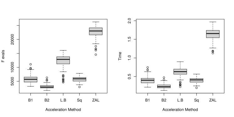
Figure 2: Quadratic minimization: number of function evaluations and runtime over $100$ random starting points.

4.2 Truncated Beta Binomial

We next consider a more difficult statistical optimization problem, turning to the cold incidence dataset by Lidwell and Sommerville, (1951). These data have been modeled as a zero-truncated beta binomial model as the reported households have at least one cold incidence. The data includes four different household types. We analyze the subset of data corresponding to all adult households here; further details on the data and results for other subsets of the data appear in Table 7 in the Appendix. Among adults, the number of households with $1,2,3,\text{ and }4$ cases are $15,5,2,\text{ and }2$ respectively.

Suppose $n$ is the total number of independent observations (households) and $x_{i}$ denotes the number of cold cases in the $i^{th}$ household. This can be modeled as a discrete probability model (Zhou et al.,, 2011) with likelihood given by

$$L(\theta|X)=\prod_{i=1}^{n}\dfrac{d(x_{i}|\theta)}{1-d(0|\theta)}\,.$$

Here $d(x|\theta)$ is the probability density function for a beta binomial distribution with parameter vector $\theta$ and maximum count of $m=4$. Here $\theta=(\alpha,\pi)$ such that $\pi\in(0,1)$ and $\alpha>0$. We use MM algorithm to numerically maximize the likelihood function. The MM updates are given by

$$\alpha_{t+1} =\dfrac{\sum_{j=0}^{m-1}(\dfrac{s_{1j}j\alpha_{t}}{\pi_{t}+j\alpha_{t}}+\dfrac{s_{2j}j\alpha_{t}}{1-\pi_{t}+j\alpha_{t}})}{\sum_{j=0}^{m-1}\dfrac{r_{j}j}{1+j\alpha_{t}}}$$

$$\pi_{t+1} =\dfrac{\sum_{j=0}^{m-1}\dfrac{s_{1j}\pi_{t}}{\pi_{t}+j\alpha_{t}}}{\sum_{j=0}^{m-1}(\dfrac{s_{1j\pi_{t}}}{\pi_{t}+j\alpha_{t}}+\dfrac{s_{2j}(1-\pi_{t})}{1-\pi_{t}+j\alpha_{t}})}$$

where $s_{1j},\,s_{2j},\,r_{j}$ can be interpreted as pseudocounts, given by

$$s_{1j} =\sum_{i=1}^{n}1_{x_{i}\geq j+1}$$

$$s_{2j} =\sum_{i=1}^{n}\left[1_{x_{i}\leq m-j-1}+\dfrac{g(0|\pi_{t},\alpha_{t})}{1-g(0|\pi_{t},\alpha_{t})}\right]$$

$$r_{j} =\sum_{i=1}^{n}\left[1+\dfrac{g(0|\pi_{t},\alpha_{t})}{1-g(0|\pi_{t},\alpha_{t})}\right]1_{t\geq j+1}\,.$$

Algorithm	-ln L	$F$ Evals	Iterations	Time (in sec)
MM	25.2283	17898	17898	0.114
BQN ($q=1$)	25.2287	26	14	0.001
BQN ($q=2$)	25.2277	29	16	0.001
L-BQN	25.2288	73	37	0.002
SqS1	25.2274	1797	1769	0.160
SqS2	25.2277	36	19	0.004
SqS3	25.2269	69	35	0.005
ZAL	25.2269	28	24	0.003

Table 3: Truncated beta binomial: performance on Lidwell and Somerville data, from initial point $(\pi,\alpha)=(0.5,1)$.

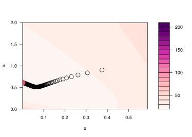
(a)

(b)

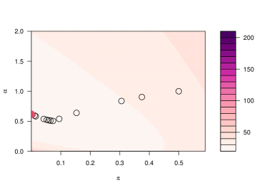
(c)

(d)

(e)

(f)

Figure 3: Truncated beta binomial: ascent paths of peer methods on the Lidwell and Somerville household incidence data in a truncated beta binomial model, with optimum marked in red.

Following Zhou et al., (2011), each algorithm is initializated at $(\pi,\alpha)=(0.5,1)$. Table 3 lists the negative log-likelihood values, number of MM evaluations (F evals), number of algorithm iterations, and runtime until convergence for each algorithm. Figure 3 provides a closer look, showing the progress path of each algorithm on a contour plot of the objective. SQUAREM methods, though achieving significant acceleration, tend to exhibit slow tail behavior near the optimal value. In particular, SQUAREM-1 leads to orders of magnitude slower convergence than the others, while it outpaced other choices of steplength among variants of SQUAREM in the simple example; we again focus on visualizing the progress of the default SQUAREM-3. In all cases, our method converges in fewer iterations and requires fewer function evaluations than its competitors despite a naive implementation. From Figure 3, we can visualize the advantage of our extrapolation-based steps making steady progress, in contrast to the more congested updates near the optimum under existing methods. While the small problem dimension does not call for a limited-memory method, we see L-BQN also compares favorably despite its streamlined updates.

4.3 Generalized eigenvalues

In this example, we consider a more complicated objective function that exhibits a zig-zag descent path under the naïve MM algorithm, rendering progress excruciatingly slow. For two $p\times p$ matrices $A$ and $B$, the generalized eigenvalue problem refers to finding a scalar $\lambda$ and a nontrivial vector $x$ such that $Ax=\lambda Bx$. We consider the case where $A$ is symmetric and $B$ is symmetric and positive definite, so that the generalized eigenvalues and eigenvectors are real (Zhou et al.,, 2011). A simple alternative for finding the generalized eigenvalues iteratively is by optimizing the Rayleigh quotient

$$R(x)=\dfrac{x^{T}Ax}{x^{T}Bx}\qquad\qquad x\neq 0\,.$$

The gradient of $R(x)$ is given by

$$\nabla R(x)=\dfrac{2}{x^{T}Bx}[Ax-R(x)Bx]\,.$$

Therefore, a solution of $\nabla R(x)=0$ corresponds to a generalized eigenpair, wherein the maximum of $R(x)$ gives the maximum generalized eigenvalue and minimum gives the minimum generalized eigenvalue. To optimize $R(x)$, we consider the line search method for steepest ascent proposed by Hestenes and Karush, (1951) as the base algorithm.

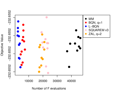
(a)

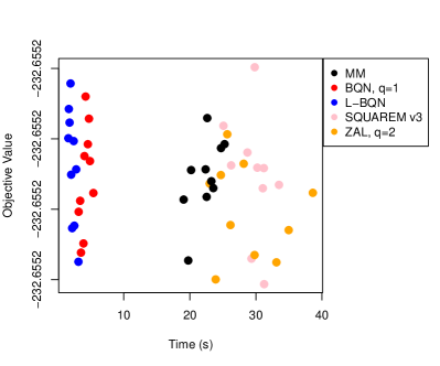
(b)

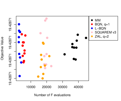
(c)

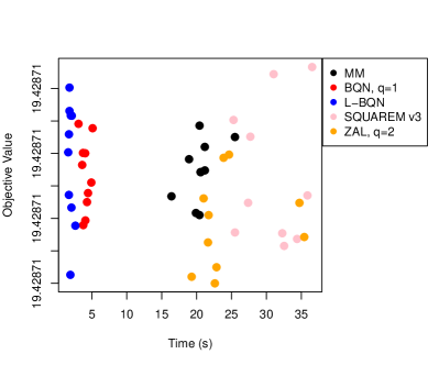
(d)

Figure 4: Generalized eigenvalues: we see all methods reach the same objective at convergence up to tolerance, plotted over $10$ restarts against the time and number of F evaluations.

	Smallest Eigenvalue			Largest Eigenvalue
Algorithm	Time (in sec)	$F$ Evals	Eigenvalue	Time (in sec)	$F$ Evals	Eigenvalue
MM	10.104	42552	-232.655	8.539	38262	19.429
BQN, $q=1$	2.046	6682	-232.655	1.854	5766	19.429
L-BQN	1.203	4046	-232.655	0.664	2399	19.429
SqS1	11.850	21777	-232.655	11.397	19642	19.429
SqS2	12.391	21777	-232.655	11.003	19642	19.429
SqS3	12.525	21777	-232.655	11.021	19642	19.429
ZAL	9.979	17920	-232.655	9.665	17415	19.429

Table 4: Generalized eigenvalues: number of $F(x)$ evaluations, runtime, and eigenvalues at convergence.

Due to the zigzag nature of steepest ascent on this problem, Zhou et al., (2011) found naïve acceleration to perform poorly. Utilizing this side information, they considered instead the $s$-fold functional composition of the base algorithm for $s$ even as the underlying map, improving performance. We refrain from using the same heuristic in order to illustrate the off-the-shelf applicability of our method. We consider a simulation study with symmetric matrices $A$ and $B$ randomly generated with $p=100$ dimensions, and run $10$ random initializations of each method from matched initial points.

Figure 4 displays objective values at convergence, and Table 4 details the results. It can be seen that without the $s$-fold functional composition, both SQUAREM and ZAL fails to accelerate meaningfully here. On the other hand, the curvature information is crucial toward informing a good search direction in such cases, and our formulation successfully leverages this information. This information is largely ignored in the scalar-based methods SQUAREM, while ZAL attempts to make use of curvature information under an assumption that it is close to the stationary point.

4.4 Multivariate t-distribution

Our last example turns to estimation under a multivariate $t$-distribution, a robust alternative to multivariate normal modeling when the errors involve heavy tails (Lange et al.,, 1989). Varadhan and Roland, (2008) considered this example to compare SQUAREM to standard EM as well as PX-EM, an efficient data augmentation method (Meng and Van Dyk,, 1997).

Suppose we have $p$-dimensional data $Y=(y_{1},...,y_{N})$ that we wish to fit to a multivariate $t$-distribution with unknown degrees of freedom $\nu$. The density is given by

$$f(y|\mu,\Sigma)\propto|\Sigma|^{-1/2}\left(\nu+(y-\mu)^{T}\Sigma^{-1}(y-\mu)\right)^{(\nu+p)/2},$$

and so the data likelihood is givein by $\prod_{i=1}^{N}f(y_{i}|\mu,\Sigma)$. There is no closed form solution to find $(\mu,\Sigma)$ which maximize the likelihood, but we can make progress by augmenting the missing data with latent variables. That is, we obtain the complete data $\{(y_{i},q_{i});i=1,...,N\}$ where q are IID from $\chi^{2}_{\nu}/\nu$; the maximum likelihood estimator (MLE) now follows from weighted least squares. In an EM algorithm, the E-step finds the expected complete data log-likelihood conditional on parameters from the previous iteration $k$. Conditional on $Y$ and $(\mu_{k},\Sigma_{k})$, the latent variables are distributed as $q_{i}\sim\chi^{2}_{\nu+p}/(\nu+d_{i}^{(k)})$, where $d_{i}^{(k)}=(y_{i}-\mu_{k})^{T}\Sigma_{k}^{-1}(y_{i}-\mu_{k});i=1,...,N$. As the complete-data log-likelihood is linear in $q_{i}$, the E-step amounts to defining

$$w_{i}=E[q_{i}|y_{i},\mu_{k},\Sigma_{k}]=(\nu+p)/(\nu+d_{i}^{(k)});\qquad i=1,...,N\,.$$

The M-step then yields:

$$\mu_{k+1} =\sum_{i}w_{i}y_{i}\bigg{/}\sum_{i}w_{i}\,,\qquad\Sigma_{k+1}\,=\,\dfrac{1}{N}w_{i}(y_{i}-\mu)(y_{i}-\mu)^{T}\,.$$

Algorithm	$F$ Evals	Time (in sec)	$-\ln L$
EM	744	1.086	8608.99
PX-EM	38	0.063	8608.99
BQN, $q=1$	112	0.215	8608.99
BQN, $q=2$	223	0.457	8608.99
L-BQN	89	0.114	8608.99
SqS1	64	0.156	8608.99
SqS2	65	0.148	8608.99
SqS3	63	0.155	8608.99
ZAL, $q=2$	383	1.383	8608.99

Table 5: Multivariate t-distribution: maximum likelihood estimation of a 25-dimensional multivariate t-distribution.

The PX-EM method of Meng and Van Dyk, (1997) differs only in the $\Sigma$ update, replacing the denominator N by $\sum_{i}w_{i}$. We randomly generate synthetic data with $\nu=1$ (a multivariate Cauchy distribution) and parameters $\mu=0$, $\Sigma=V$, where $V$ is a symmetric randomly generated matrix with dimension $p=25$, which corresponds to $350$ parameters (25 for $\mu$ and 325 for $\Sigma$). We report results obtained from following the initial values suggested by Meng and Van Dyk, (1997):

$$\mu_{0}=\dfrac{1}{N}\sum_{i=1}^{N}y_{i},\qquad\Sigma_{0}=\dfrac{1}{N}\sum_{i=1}^{N}(y_{i}-\overline{y})(y_{i}-\overline{y})^{T}\,.$$

Table 5 displays runtime, number of $F$ evaluations (F evals), and negative log likelihood of all acceleration schemes at convergence. Our method achieves significant acceleration compared to the standard EM algorithm. However, it does not compare well with SQUAREM in this high-dimensional setting. Note that L-BQN performs on par with SQUAREM. Here ZAL fails to provide meaningful acceleration under its implementation in turboEM—we observe it frequently proposes an update such that $\Sigma_{k}$ is not positive-definite. In these cases, the algorithm reverts to the default MM update, adding additional computational effort, though the implementation in Zhou et al., (2011) achieves more success. Though performance is always quite dependent on implementations, we echo the overall theme in the findings of Varadhan and Roland, (2008); Zhou et al., (2011) that model-specific augmentation under PX-EM performs remarkably well, outpacing all of the more general methods. This example illustrates that despite the robust performance of our proposed method across settings, it is worthwhile to exploit problem-specific structure as does PX-EM whenever possible.

5 Conclusion

This article presents a novel quasi-Newton acceleration of MM algorithms that extends recent ideas, but lends them new intuition as well as theoretical guarantees. The method retains gradient information across all components, which is often ignored in other pure MM accelerators. A key advantage of MM algorithms is their transfer of difficulty away from the original objective function, obtained by the construction of surrogates. While the hybrid quasi-Newton MM accelerators (Lange,, 1995; Heiser,, 1995; Lange et al.,, 2000) are rigorously analyzed in the literature, they lose this appeal in part by requiring information from the original objective through their iterates. Our approach seeks to embody the best of both worlds, retaining the simplicity of pure accelerators without restrictive assumptions, maintaining computational tractability so that it is amenable for large and high-dimensional problems, and taking advantage of richer curvature information that yields classical convergence guarantees which may not hold for its peer methods.

The limited-memory version of our method performs well on our representative, but not exhaustive, set of examples. As this shows promise toward high-dimensional problems, a fruitful line of research may seek to study the convergence properties of L-BQN explicitly, building on prior analyses on convergence of limited memory BFGS method (Liu and Nocedal,, 1989). Exploring optimal step size selection presents another open direction (Nocedal and Wright,, 2006). Despite deriving from a different perspective, it is satisfying that the steplength for our inverse Jacobian update in Eq.(9) reveals that used for the first version of STEM as a special case Varadhan and Roland, (2008). Nonetheless, exploring the practical and theoretical merits of alternatives may reap further advantages.

6 Appendix

6.1 Proof of Theorem 1

Let $\mathbb{R}^{p\times p}$ denote linear space of real matrices of order $p\times p$. Recall that $\|A\|_{M}\mathrel{\mathop{\mathchar 58\relax}}=\|MAM\|_{F}$ is a matrix norm of matrix $A$ for any matrix $M$, $\|\cdot\|_{F}$ is the Frobenius norm, and $\|\cdot\|$ denotes a vector norm or its induced operator norm.

.

The proof argues that if $\boldsymbol{x}_{0}\in D$, then $\boldsymbol{x}_{1}$ also lies in D using the inequality in Eq.(13). Additionally, it is shown that the distance of $\boldsymbol{x}_{1}$ from $\boldsymbol{x}^{\ast}$ is less than or equal to some $r$th fraction of the distance of $\boldsymbol{x}_{0}$ from $\boldsymbol{x}^{\ast}$. By induction, we prove that $\boldsymbol{x}_{i}\in D$ for all $i\geq 1$, and eventually converge to $\boldsymbol{x}^{\ast}$ with $r$ rate of convergence.

To this end, we upper bound the norm of the Jacobian and inverse Jacobian matrices at $\boldsymbol{x}^{\ast}$ as $\|dG(\boldsymbol{x}^{\ast})\|\leq\sigma\text{ and }\|dG(\boldsymbol{x}^{\ast})^{-1}\|\leq\gamma$. For any $r\in(0,1)$, we can choose $\epsilon(r)=\epsilon\text{ and }\delta(r)=\delta$ such that

$$[2\alpha_{1}\delta+\alpha_{2}]\dfrac{\epsilon^{d}}{1-r^{d}} \leq\delta$$ (15)

$$2\sigma\delta\eta+(\gamma+2\eta\delta)K\epsilon^{d} \leq r\,.$$ (16)

If necessary, we may further restrict $\epsilon$ and $\delta$ such that $(\boldsymbol{x},H)\in N$ whenever $\|\boldsymbol{x}-\boldsymbol{x}^{\ast}\|<\epsilon$ and $\|H-dG(\boldsymbol{x}^{\ast})^{-1}\|_{M}~{}<~{}2\delta$. Now suppose $\|\boldsymbol{x}_{0}-\boldsymbol{x}^{\ast}\|<\epsilon\text{ and }\|H_{0}-dG(\boldsymbol{x}^{\ast})^{-1}\|_{M}<\delta$. Then $\|H_{0}-dG(\boldsymbol{x}^{\ast})^{-1}\|<\eta\delta<2\eta\delta$ by the equivalence of norms in finite-dimensional vector spaces. From Eq.(16), $2\sigma\delta\eta\leq 2r$, and therefore the Banach lemma gives,

$$\|H_{0}^{-1}\|\leq\dfrac{\sigma}{1-r}\,.$$

Now, we will show that if $\boldsymbol{x}_{0}\in D$, then $\boldsymbol{x}_{1}$ also lies in $D$. For this purpose, we add and subtract $H_{0}dG(\boldsymbol{x}^{\ast})(\boldsymbol{x}_{0}-\boldsymbol{x}^{\ast})$ and add the null term $H_{0}G(\boldsymbol{x}^{\ast})$ to the known update formulation for $\boldsymbol{x}_{1}$ giving

$$\boldsymbol{x}_{1}-\boldsymbol{x}^{\ast} =\boldsymbol{x}_{0}-H_{0}G(\boldsymbol{x}_{0})-\boldsymbol{x}^{\ast}$$

$$=-H_{0}\left[G(\boldsymbol{x}_{0})-G(\boldsymbol{x}^{\ast})-dG(\boldsymbol{x}^{\ast})(\boldsymbol{x}_{0}-\boldsymbol{x}^{\ast})\right]+\left[I_{p}-H_{0}dG(\boldsymbol{x}^{\ast})\right](\boldsymbol{x}_{0}-\boldsymbol{x}^{\ast})\,.$$

Using the fact that $\|I_{p}-H_{0}dG(\boldsymbol{x}^{\ast})\|=\|dG(\boldsymbol{x}^{\ast})(H_{0}-dG(\boldsymbol{x}^{\ast})^{-1})\|\leq\|dG(\boldsymbol{x}^{\ast})\|\|H_{0}-dG(\boldsymbol{x}^{\ast})^{-1}\|\leq\sigma(2\delta\eta)$ and Inequality (1),

$$\|\boldsymbol{x}_{1}-\boldsymbol{x}^{\ast}\| \leq\|H_{0}\|K\epsilon^{d}\|\boldsymbol{x}_{0}-\boldsymbol{x}^{\ast}\|+2\sigma\delta\eta\|\boldsymbol{x}_{0}-\boldsymbol{x}^{\ast}\| =\left[\|H_{0}\|K\epsilon^{d}+2\sigma\epsilon\delta\eta\right]\|\boldsymbol{x}_{0}-\boldsymbol{x}^{\ast}\|\,.$$

But $\|H_{0}\|\leq\|H_{0}-dG(\boldsymbol{x}^{\ast})^{-1}\|+\|dG(\boldsymbol{x}^{\ast})^{-1}\|\leq 2\eta\delta+\gamma$. Therefore,

$$\|\boldsymbol{x}_{1}-\boldsymbol{x}^{\ast}\|\leq[(2\eta\delta+\gamma)K\epsilon^{d}+2\sigma\epsilon\delta\eta]\|\boldsymbol{x}_{0}-\boldsymbol{x}^{\ast}\|\leq r\|\boldsymbol{x}_{0}-\boldsymbol{x}^{\ast}\|$$

using the inequality in Eq.(16), and hence $\boldsymbol{x}_{1}\in D$. The rest of the proof proceeds by induction. Assume that $\|H_{k}-dG(\boldsymbol{x}^{\ast})^{-1}\|_{M}<2\delta$, which implies $H_{k}\in N_{2}$ and $\|\boldsymbol{x}_{k+1}-\boldsymbol{x}^{\ast}\|\leq r\|\boldsymbol{x}_{k}-\boldsymbol{x}^{\ast}\|$ for $k=0,1,\dots,m-1$. Now since $\boldsymbol{x}_{k}\in N_{1}\subseteq S$, we have $\|F(\boldsymbol{x}_{k})-\boldsymbol{x}^{\ast}\|^{d}\leq\tau^{d}\|\boldsymbol{x}_{k}-\boldsymbol{x}^{\ast}\|^{d}$ by the local convergence of the MM algorithm in $S$. It follows from the inequality in Eq.(13) that

$$\|H_{k+1}-dG(\boldsymbol{x}^{\ast})^{-1}\|_{M}-\|H_{k}-dG(\boldsymbol{x}^{\ast})^{-1}\|_{M} \leq\alpha_{1}\|\boldsymbol{x}_{k}-\boldsymbol{x}^{\ast}\|^{d}\|H_{k}-dG(\boldsymbol{x}^{\ast})^{-1}\|_{M}+\alpha_{2}\|\boldsymbol{x}_{k}-\boldsymbol{x}^{\ast}\|^{d}$$

$$\leq\alpha_{1}(r^{kd}\epsilon^{d})(2\delta)+\alpha_{2}r^{kd}\epsilon^{d}\,.$$

Therefore, from the inequality in Eq.(15), we have

$$\|H_{m}-dG(\boldsymbol{x}^{\ast})^{-1}\|_{M}\leq\|H_{0}-dG(\boldsymbol{x}^{\ast})^{-1}\|_{M}+(2\alpha_{1}\delta+\alpha_{2})\dfrac{\epsilon^{d}}{1-r^{d}}\leq 2\delta\,.$$

In this way, the induction step is completed by following the same proof as the case for $m=1$. In particular, since $\|H_{m}-dG(\boldsymbol{x}^{\ast})^{-1}\|\leq 2\eta\delta$, the Banach lemma implies that

$$\|H_{m}^{-1}\|\leq\dfrac{\sigma}{1-r}\,.$$

∎

6.2 Proof of Theorem 2

In order to show that our algorithm satisfies (13) for meeting the conditions of Theorem 1, we write (9) as

$$\bar{E}=E\left[I_{p}-\dfrac{M^{-1}\boldsymbol{v}(M\boldsymbol{v})^{T}}{\|\boldsymbol{v}\|^{2}}\right]+\dfrac{M(\boldsymbol{u}-dG(\boldsymbol{x}^{\ast})^{-1}v)(M\boldsymbol{v})^{T}}{\|\boldsymbol{v}\|^{2}},$$ (17)

where $\bar{E}=M(\bar{H}-dG(\boldsymbol{x}^{\ast})^{-1})M\text{ and }E=M(H-dG(\boldsymbol{x}^{\ast})^{-1})M$. Eq.(17) will allow us to derive the relationship between $\|H-dG(\boldsymbol{x}^{\ast})^{-1}\|_{M}$ and $\|\bar{H}-dG(\boldsymbol{x}^{\ast})^{-1}\|_{M}$ satisfying the inequality in (13). For this purpose, we present the following technical lemma with four important inequalities satisfied by our algorithm. Since our update formulation falls in the classical line of thought, we inherit the following properties directly from the analysis presented by Broyden et al., (1973), so the proofs have been omitted. Nonetheless, the results have been included for the sake of completion for Theorem 2.

Lemma 2.

Let $M\in\mathbb{R}^{p\times p}$ be a non-singular symmetric matrix such that

$$\|M\boldsymbol{c}-M^{-1}\boldsymbol{d}\|\leq\beta\|M^{-1}\boldsymbol{d}\|$$ (18)

for some $\beta\in[0,1/3]$ and vectors $\boldsymbol{c}$ and $\boldsymbol{d}$ in $\mathbb{R}^{p}$ with $\boldsymbol{d}\neq\mathbf{0}$. Then using $E$ and $\bar{E}$ as defined earlier,

1. $(1-\beta)\|M^{-1}\boldsymbol{d}\|^{2}\leq\boldsymbol{c}^{T}\boldsymbol{d}\leq(1+\beta)\|M^{-1}\boldsymbol{d}\|^{2}$ .

2. $E\left[I-\dfrac{(M^{-1}\boldsymbol{d}(M^{-1}\boldsymbol{d})^{T}}{\boldsymbol{c}^{T}\boldsymbol{d}}\right]\leq\sqrt{1-\alpha\theta^{2}}\|E\|_{F}$ .

3. $\left\|E\left[I-\dfrac{M^{-1}\boldsymbol{d}(M\boldsymbol{c})^{T}}{\boldsymbol{c}^{T}\boldsymbol{d}}\right]\right\|_{F}\leq\left[\sqrt{1-\alpha\theta^{2}}+(1-\beta)^{-1}\dfrac{\|M\boldsymbol{c}-M^{-1}\boldsymbol{d}\|}{\|M^{-1}\boldsymbol{d}\|}\right]\|E\|_{F}$ ,
   where

   $$\alpha=\dfrac{1-2\beta}{1-\beta^{2}}\in[3/8,1]$$

   and

   $$\theta=\dfrac{\|EM^{-1}\boldsymbol{d}\|}{\|E\|_{F}\|M^{-1}\boldsymbol{d}\|}\in[0,1]\,.$$

   Moreover, for any $\boldsymbol{a}\in\mathbb{R}^{p}$,

4. $\left\|\dfrac{(\boldsymbol{a}-dG(\boldsymbol{x}^{\ast})^{-1}\boldsymbol{d})(M\boldsymbol{c})^{T}}{\boldsymbol{c}^{T}\boldsymbol{d}}\right\|_{F}\leq 2\dfrac{\|\boldsymbol{a}-dG(\boldsymbol{x}^{\ast})^{-1}\boldsymbol{d}\|}{\|M^{-1}\boldsymbol{d}\|}$ .

In the following proof, we will use results from the above lemma with $\boldsymbol{c}=\boldsymbol{v}$, $\boldsymbol{d}=\boldsymbol{v}$, and result $(d)$ particularly for $\boldsymbol{a}=\boldsymbol{u}$. We are now ready to show that the conditions of Theorem 1 are satisfied by our update formula. This allows us to construct the exact neighborhood for each $r\in(0,1)$ wherein our algorithm converges to the stationary point with rate $r$.

Theorem 2.

Firstly, we construct the neighborhoods $N_{1}$ and $N_{2}$ wherein our the updates in (1) and (9) are well-defined. Define $N_{2}=\{H\in\mathbb{R}^{p\times p}\mathrel{\mathop{\mathchar 58\relax}}\|dG(\boldsymbol{x}^{\ast})\|\|H-dG(\boldsymbol{x}^{\ast})^{-1}\|<1/2\}$ such that each $H\in N_{2}$ is non-singular, and there exists a constant $\nu>0$ such that $\|H\|\leq\nu$ for all $H\in N_{2}$. Using Lemma 1, we we also choose $\epsilon\text{ and }\rho$ such that $\max\{\|\bar{\boldsymbol{x}}-\boldsymbol{x}^{\ast}\|^{d},\|\boldsymbol{x}-\boldsymbol{x}^{\ast}\|^{d}\}\leq\epsilon$ implies that (12) holds. In particular, if $\|\boldsymbol{x}-\boldsymbol{x}^{\ast}\|\leq\epsilon$ and $H\in N_{2}$, then $\boldsymbol{x}\in D$ and

$$(1/\rho)\|\boldsymbol{x}-\boldsymbol{x}^{\ast}\|\leq\|G(\boldsymbol{x})\|\leq\rho\|\boldsymbol{x}-\boldsymbol{x}^{\ast}\|\,.$$

As a consequence of applying the inequality above on Eq.(1), we have

$$\|\boldsymbol{s}\|\leq\|H\|\|G(\boldsymbol{x})\|\leq\rho\|H\|\|\boldsymbol{x}-\boldsymbol{x}^{\ast}\|\leq\rho\nu\|\boldsymbol{x}-\boldsymbol{x}^{\ast}\|\,.$$

Now define $N_{1}$ as the set of all $\boldsymbol{x}\in\mathbb{R}^{p}$ such that

$$\|\boldsymbol{x}-\boldsymbol{x}^{\ast}\|<\min\{\epsilon/2,\epsilon/(2\rho),\epsilon/(2\rho\nu)\}$$

where $\rho\epsilon<(3\mu_{2})^{-1/d}$. Now if $\boldsymbol{x}\in N_{1}$ then

$$\|\boldsymbol{s}\| \leq\rho\nu\|\boldsymbol{x}-\boldsymbol{x}^{\ast}\|\leq\epsilon/2\qquad\text{ and }\qquad\|F(\boldsymbol{x})-\boldsymbol{x}\|\leq\rho\|\boldsymbol{x}-\boldsymbol{x}^{\ast}\|\leq\epsilon/2\,.$$ (19)

If $N=((N_{1}\cap S)\times N_{2})\cap N^{\prime}$ and $(\boldsymbol{x},H)\in N$, then $\boldsymbol{x},\bar{\boldsymbol{x}},\text{ and }F(\boldsymbol{x})$ lie in $D$ because using (19)

$$\|\bar{\boldsymbol{x}}-\boldsymbol{x}^{\ast}\|\leq\|\boldsymbol{s}\|+\|\boldsymbol{x}-\boldsymbol{x}^{\ast}\|\leq\epsilon\quad\text{and}\quad\|\bar{F(\boldsymbol{x})}-\boldsymbol{x}^{\ast}\|\leq\|F(\boldsymbol{x})-\boldsymbol{x}\|+\|\boldsymbol{x}-\boldsymbol{x}^{\ast}\|\leq\epsilon\,.$$

Hence Inequality (12) shows that

$$\left(\dfrac{1}{\rho}\right)\|\boldsymbol{s}\| \leq\|\boldsymbol{y}\|\leq\rho\|\boldsymbol{s}\|\,,$$ (20a)

$$\left(\dfrac{1}{\rho}\right)\|\boldsymbol{u}\| \leq\|\boldsymbol{v}\|\leq\rho\|\boldsymbol{u}\|\,,$$ (20b)

and in particular

$$\mu_{2}\|\boldsymbol{y}\|^{d} \leq\mu_{2}(\rho\epsilon)^{d}\leq 1/3$$ (21a)

$$\mu_{2}\|\boldsymbol{v}\|^{d} \leq\mu_{2}(\rho\epsilon)^{d}\leq 1/3\,.$$ (21b)

Thus $\boldsymbol{y}=0$ if and only if $\boldsymbol{s}=0$, which happens if and only if $\boldsymbol{x}=\boldsymbol{x}^{\ast}$. This shows that the update function in Eq.(1) and (9) is well-defined for all $(\boldsymbol{x},H)\in N$. We now show that the update functions satisfy the conditions of Theorem 1. Since (14) and (21b) imply that (18) hold with $\beta=1/3$, it follows from (14) and parts $(c)$, $(d)$ of Lemma 2 applied on (17) that

$$\|\bar{H}-dG(\boldsymbol{x}^{\ast})^{-1}\|_{M} \leq\left[\sqrt{1-\dfrac{3}{8}\theta^{2}}+\dfrac{3}{2}\mu_{2}\|\boldsymbol{v}\|^{d}\right]\|H-dG(\boldsymbol{x}^{\ast})^{-1}\|_{M}$$

$$\qquad+\dfrac{2\|M\|\|\boldsymbol{u}-dG(\boldsymbol{x}^{\ast})^{-1}\boldsymbol{v}\|}{\|M^{-1}\boldsymbol{v}\|}$$

where $\theta=\dfrac{\|M[H-dG(\boldsymbol{x}^{\ast})^{-1}]\boldsymbol{v}\|}{\|H-dG(\boldsymbol{x}^{\ast})^{-1}\|_{M}\|M^{-1}\boldsymbol{v}\|}$. But for any $\boldsymbol{x}\in N_{1}$,

$$\|\boldsymbol{u}-dG(\boldsymbol{x}^{\ast})^{-1}\boldsymbol{v}\|\leq K\|dG(\boldsymbol{x}^{\ast})^{-1}\|\max\{\|F(\boldsymbol{x})-\boldsymbol{x}^{\ast}\|^{d},\|\boldsymbol{x}-\boldsymbol{x}^{\ast}\|^{d}\}\|\boldsymbol{u}\|\,.$$

Using Inequality (20b),

$$\|\bar{H}-dG(\boldsymbol{x}^{\ast})^{-1}\|_{M} \leq\sqrt{1-\dfrac{3}{8}\theta^{2}}\|H-dG(\boldsymbol{x}^{\ast})^{-1}\|_{M}$$

$$\qquad+\max\{\|F(\boldsymbol{x})-\boldsymbol{x}^{\ast}\|^{d},\|\boldsymbol{x}-\boldsymbol{x}^{\ast}\|^{d}\}[\alpha_{1}\|H-dG(\boldsymbol{x}^{\ast})^{-1}\|_{M}+\alpha_{2}]$$ (22)

where $\alpha_{1}=\left(\dfrac{2}{3}\right)(2\rho)^{d}\mu_{2}$ and $\alpha_{2}=2\rho K\|M\|^{2}\|dG(\boldsymbol{x}^{\ast})^{-1}\|$. This inequality now satisfies the assumptions of Theorem 1 and therefore, $\boldsymbol{x}_{k}$ converges locally to $\boldsymbol{x}^{\ast}$ as $k$ increases.

∎

Proof of Corollary 2.

To prove the Q-superlinear convergence, we use the Corollary 1 that guarantees the desired result if a subsequence of $\{H_{k}\}$ converges to $dG(\boldsymbol{x}^{\ast})^{-1}$. Define

$$\theta_{k}=\dfrac{\|M[H_{k}-dG(\boldsymbol{x}^{\ast})^{-1}]\boldsymbol{v}_{k}\|}{\|H_{k}-dG(\boldsymbol{x}^{\ast})^{-1}\|_{M}\|M^{-1}\boldsymbol{v}_{k}\|}\,.$$

Since $\sqrt{1-\alpha}<1-\alpha/2$, from Eq.(6.2) we get

$$\dfrac{3}{16}\theta_{k}^{2}\|H-dG(\boldsymbol{x}^{\ast})^{-1}\|_{M} \leq\left[\|H-dG(\boldsymbol{x}^{\ast})^{-1}\|_{M}-\|\bar{H}-dG(\boldsymbol{x}^{\ast})^{-1}\|_{M}\right]$$

$$\qquad+\max\left\{\|F(\boldsymbol{x})-\boldsymbol{x}^{\ast}\|^{d},\|\boldsymbol{x}-\boldsymbol{x}^{\ast}\|^{d}\right\}[\alpha_{1}\|H-dG(\boldsymbol{x}^{\ast})^{-1}\|_{M}+\alpha_{2}]\,.$$ (23)

If there is a subsequence $\{H_{k}\}$ such that it converges to $dG(\boldsymbol{x}^{\ast})^{-1}$, then $\|H-dG(\boldsymbol{x}^{\ast})^{-1}\|_{M}$ converges to zero and we are done by Corollary 1. Otherwise, $\|H-dG(\boldsymbol{x}^{\ast})^{-1}\|_{M}$ is bounded by $\alpha$ but does not converge to zero. Now summation on Eq.(6.2) yields

$$\dfrac{3}{16}\sum_{k=1}^{\infty}\theta_{k}^{2}\|H_{k}-dG(\boldsymbol{x}^{\ast})^{-1}\|_{M} \leq\|H_{0}-dG(\boldsymbol{x}^{\ast})^{-1}\|_{M}-\|H_{\infty}-dG(\boldsymbol{x}^{\ast})^{-1}\|_{M}$$

$$+[\alpha_{1}\alpha+\alpha_{2}]\epsilon^{d}\sum_{k=1}^{\infty}r^{(k-1)d}$$

$$\leq 2\alpha+\dfrac{[\alpha_{1}\alpha+\alpha_{2}]\epsilon^{d}}{1-r^{d}}<\infty\,.$$

and since

$$\sum_{k=1}^{\infty}\theta_{k}^{2}\|H_{k}-dG(\boldsymbol{x}^{\ast})^{-1}\|_{M} =\sum_{k=1}^{\infty}\dfrac{\|M[H_{k}-dG(\boldsymbol{x}^{\ast})^{-1}]\boldsymbol{v}_{k}\|^{2}}{\|H_{k}-dG(\boldsymbol{x}^{\ast})^{-1}\|_{M}\|M^{-1}\boldsymbol{v}_{k}\|^{2}}$$

$$\geq\dfrac{1}{\alpha}\sum_{k=1}^{\infty}\dfrac{\|M[H_{k}-dG(\boldsymbol{x}^{\ast})^{-1}]\boldsymbol{v}_{k}\|^{2}}{\|M^{-1}\boldsymbol{v}_{k}\|^{2}}\,,$$

this forces the following limit to converge to zero.

$$\lim_{k\to\infty}\dfrac{\|[H_{k}-dG(\boldsymbol{x}^{\ast})^{-1}]\boldsymbol{v}_{k}\|}{\|\boldsymbol{v}_{k}\|}=0\,.$$ (24)

Using $H_{k}\boldsymbol{v}_{k}=H_{k}G(F(\boldsymbol{x}_{k}))-H_{k}G(\boldsymbol{x}_{k})=H_{k}G(F(\boldsymbol{x}_{k}))+\boldsymbol{s}_{k}$, we can write

$$[H_{k}-dG(\boldsymbol{x}^{\ast})^{-1}]\boldsymbol{v}_{k}=H_{k}G(F(\boldsymbol{x}_{k}))-dG(\boldsymbol{x}^{\ast})^{-1}[\boldsymbol{v}_{k}-dG(\boldsymbol{x}^{\ast})s_{k}]\,.$$

At the end of the proof of Theorem 1, we prove that there exists $\upsilon>0$ such that $\|H_{k}\|\leq\upsilon$. Using the above equation, Lemma 1, and the fact that $\|\boldsymbol{x}_{k+1}-\boldsymbol{x}^{\ast}\|\leq\|\boldsymbol{x}_{k}-\boldsymbol{x}^{\ast}\|$, we get

$$\|G(F(\boldsymbol{x}_{k}))\| \leq\|H_{k}^{-1}\|\left[\|[H_{k}-dG(\boldsymbol{x}^{\ast})^{-1}]\boldsymbol{v}_{k}\|+\|dG(\boldsymbol{x}^{\ast})^{-1}\|\|\boldsymbol{v}_{k}-dG(\boldsymbol{x}^{\ast})\boldsymbol{s}_{k}\|\right]$$

$$\leq\upsilon\big{[}\|[H_{k}-dG(\boldsymbol{x}^{\ast})^{-1}]\boldsymbol{v}_{k}\|+\|dG(\boldsymbol{x}^{\ast})^{-1}\|K\|\boldsymbol{x}_{k}-\boldsymbol{x}^{\ast}\|^{d}\|\boldsymbol{u}_{k}\|$$

$$\qquad+\|dG(\boldsymbol{x}^{\ast})^{-1}\|\|G^{\prime}(\boldsymbol{x}^{\ast})(\boldsymbol{s}_{k}-\boldsymbol{u}_{k})\|\big{]}$$

$$\leq\upsilon\big{[}\|[H_{k}-dG(\boldsymbol{x}^{\ast})^{-1}]\boldsymbol{v}_{k}\|+\|dG(\boldsymbol{x}^{\ast})^{-1}\|K\|\boldsymbol{x}_{k}-\boldsymbol{x}^{\ast}\|^{d}\|\boldsymbol{u}_{k}\|$$

$$\qquad+\|dG(\boldsymbol{x}^{\ast})^{-1}\|\|dG(\boldsymbol{x}^{\ast})\|\|(\boldsymbol{x}_{k+1}-F(\boldsymbol{x}_{k}))\|\big{]}\,.$$ (25)

A critical assumption is the condition that $\lim_{k\to\infty}\|\boldsymbol{x}_{k+1}-F(\boldsymbol{x}_{k})\|/\|\boldsymbol{x}_{k}-\boldsymbol{x}^{\ast}\|=0$. Since $\|\boldsymbol{u}_{k}\|\geq(1/\rho)\|\boldsymbol{v}_{k}\|$ and appealing to the limit in Eq.(24),

$$\lim_{k\to\infty}\dfrac{\|G(F(\boldsymbol{x}_{k}))\|}{\|\boldsymbol{u}_{k}\|}=0.$$

Now using Eq.(12), we know that $\|F(\boldsymbol{x}_{k})-\boldsymbol{x}^{\ast}\|\leq\rho\|G(F(\boldsymbol{x}_{k}))\|$ and $\|\boldsymbol{x}_{k}-\boldsymbol{x}^{\ast}\|\geq\|\boldsymbol{u}_{k}\|/\rho$. Therefore we have the string of inequalities

$$\dfrac{\|\boldsymbol{x}_{k+1}-\boldsymbol{x}^{\ast}\|}{\|\boldsymbol{x}_{k}-\boldsymbol{x}^{\ast}\|}\leq\dfrac{\|\boldsymbol{x}_{k+1}-F(\boldsymbol{x}_{k})\|}{\|\boldsymbol{x}_{k}-\boldsymbol{x}^{\ast}\|}+\dfrac{\|F(\boldsymbol{x}_{k})-\boldsymbol{x}^{\ast}\|}{\|\boldsymbol{x}_{k}-\boldsymbol{x}^{\ast}\|}\leq\dfrac{\|\boldsymbol{x}_{k+1}-F(\boldsymbol{x}_{k})\|}{\|\boldsymbol{x}_{k}-\boldsymbol{x}^{\ast}\|}+\dfrac{\rho^{2}\|G(F(\boldsymbol{x}_{k}))\|}{\|\boldsymbol{u}_{k}\|}\,.$$

Q-superlinearity follows as the upperbound of ${\|\boldsymbol{x}_{k+1}-\boldsymbol{x}^{\ast}\|}/{\|\boldsymbol{x}_{k}-\boldsymbol{x}^{\ast}\|}$ goes to $0$ as $k\to\infty$. This concludes the proof of Q-superlinearity of our quasi-Newton method for MM acceleration in a neighborhood of the limit point. ∎

6.3 Examples

6.3.1 Truncated Beta Binomial

As discussed earlier in Example 4.2, we have the Lidwell and Sommerville, (1951) dataset of cold incidences in households of size four. These holuseholds are classified as: (a) adults only, (b) adults and school children, (c) adults and infants, and (d) adults, school children, and infants. Only households with at least one cold incidence are reported, hence warranting the use of zero-truncated beta-binomial distribution to model the dataset.

We have already presented a comparative analysis of different MM acceleration methods for dataset subcategory (a) in Table 3. Using the same tolerance $\epsilon$ and starting points $(\pi_{0},\alpha_{0})$, we run the methods for the other three subcategories and present the unified results in Table 7. It is worth to note that while at least one SQUAREM methods fail to provide acceleration for each subcategory, BQN consistently accelerates over the slow MM algorithm.

Household	Number of cases				MLE
	1	2	3	4	$\hat{\pi}$	$\hat{\alpha}$
(a)	15	5	2	2	0.0000	0.6151
(b)	12	6	7	6	0.1479	1.1593
(c)	10	9	2	7	0.0000	1.6499
(d)	26	15	3	9	0.0001	1.0594

Table 6: The Lidwell and Somerville (1951) cold data on households of size $4$ and corresponding MLEs under the truncated beta-binomial model.

Table 7: Truncated beta binomial: comparison of algorithms for the Lidwell and Somerville Data. The starting point is $(\pi,\alpha)=(0.5,1)$, the stopping criterion is $\epsilon=10^{-7}$, and the number of parameters is two.

Data Algorithm -ln L Fevals Iterations Time (in sec) (b) MM 41.7286 5492 5492 0.026 BQN, $q=1$ 41.7286 1012 507 0.036 SqS1 41.7286 248 210 0.019 SqS2 41.7286 1553 1148 0.106 SqS3 41.7286 79 40 0.006 ZAL, $q=2$ 41.7286 1136 1132 0.063 (c) MM 37.3586 61843 61843 0.323 BQN, $q=1$ 37.3589 1864 933 0.062 SqS1 37.3587 1370 1345 0.122 SqS2 37.3582 9649 8966 0.977 SqS3 37.3582 145 73 0.010 ZAL, $q=2$ 37.3582 28 24 0.004 (d) MM 65.0423 25026 25026 0.132 BQN, $q=1$ 65.0435 268 135 0.007 SqS1 65.0413 1648 1622 0.136 SqS2 65.0420 5727 5443 0.472 SqS3 65.0402 97 49 0.007 ZAL, $q=2$ 65.0402 25 21 0.003

References

- Boyles, (1983) Boyles, R. A. (1983). On the convergence of the EM algorithm. Journal of the Royal Statistical Society: Series B (Methodological), 45(1):47–50.
- Broyden, (1965) Broyden, C. G. (1965). A class of methods for solving nonlinear simultaneous equations. Mathematics of Computation, 19(92):577–593.
- Broyden et al., (1973) Broyden, C. G., Dennis Jr, J., and Moré, J. J. (1973). On the local and superlinear convergence of quasi-Newton methods. IMA Journal of Applied Mathematics, 12(3):223–245.
- Defazio et al., (2014) Defazio, A., Bach, F., and Lacoste-Julien, S. (2014). SAGA: a fast incremental gradient method with support for non-strongly convex composite objectives. In Proceedings of the 27th International Conference on Neural Information Processing Systems-Volume 1, pages 1646–1654.
- Dempster et al., (1977) Dempster, A. P., Laird, N. M., and Rubin, D. B. (1977). Maximum likelihood from incomplete data via the EM algorithm. Journal of the Royal Statistical Society: Series B (Methodological), 39(1):1–22.
- Dennis Jr and Schnabel, (1996) Dennis Jr, J. E. and Schnabel, R. B. (1996). Numerical methods for unconstrained optimization and nonlinear equations. SIAM.
- Everitt, (2012) Everitt, B. (2012). Introduction to optimization methods and their application in statistics.
- Fletcher, (2013) Fletcher, R. (2013). Practical Methods of Optimization. John Wiley & Sons.
- Griewank and Toint, (1982) Griewank, A. and Toint, P. L. (1982). Partitioned variable metric updates for large structured optimization problems. Numerische Mathematik, 39(1):119–137.
- Heiser, (1995) Heiser, W. J. (1995). Convergent computation by iterative majorization: Theory and applications in multidimensional data analysis. Recent Advances in Descriptive Multivariate Analysis, pages 157–189.
- Hestenes and Karush, (1951) Hestenes, M. and Karush, W. (1951). Solutions of A=B. J. Res. Nat. Bur. Standards, 47:471–478.
- Jamshidian and Jennrich, (1993) Jamshidian, M. and Jennrich, R. I. (1993). Conjugate gradient acceleration of the EM algorithm. Journal of the American Statistical Association, 88(421):221–228.
- Jamshidian and Jennrich, (1997) Jamshidian, M. and Jennrich, R. I. (1997). Acceleration of the EM algorithm by using quasi-Newton methods. Journal of the Royal Statistical Society: Series B (Statistical Methodology), 59(3):569–587.
- Laird, (1978) Laird, N. (1978). Nonparametric maximum likelihood estimation of a mixing distribution. Journal of the American Statistical Association, 73(364):805–811.
- Lange, (1995) Lange, K. (1995). A quasi-Newton acceleration of the EM algorithm. Statistica Sinica, pages 1–18.
- Lange, (2016) Lange, K. (2016). MM optimization algorithms. SIAM.
- Lange et al., (2000) Lange, K., Hunter, D. R., and Yang, I. (2000). Optimization transfer using surrogate objective functions. Journal of Computational and Graphical Statistics, 9(1):1–20.
- Lange and Wu, (2008) Lange, K. and Wu, T. (2008). An MM algorithm for multicategory vertex discriminant analysis. Journal of Computational and Graphical Statistics, 17(3):527–544.
- Lange et al., (1989) Lange, K. L., Little, R. J., and Taylor, J. M. (1989). Robust statistical modeling using the t distribution. Journal of the American Statistical Association, 84(408):881–896.
- Lee and Seung, (1999) Lee, D. D. and Seung, H. S. (1999). Learning the parts of objects by non-negative matrix factorization. Nature, 401(6755):788–791.
- Lidwell and Sommerville, (1951) Lidwell, O. and Sommerville, T. (1951). Observations on the incidence and distribution of the common cold in a rural community during 1948 and 1949. Epidemiology & Infection, 49(4):365–381.
- Lin et al., (2017) Lin, H., Mairal, J., and Harchaoui, Z. (2017). A generic quasi-Newton algorithm for faster gradient-based optimization.
- Liu and Nocedal, (1989) Liu, D. C. and Nocedal, J. (1989). On the limited memory BFGS method for large scale optimization. Mathematical Programming, 45(1):503–528.
- Luenberger et al., (1984) Luenberger, D. G., Ye, Y., et al. (1984). Linear and Nonlinear Programming, volume 2. Springer.
- Meng and Rubin, (1994) Meng, X.-L. and Rubin, D. B. (1994). On the global and componentwise rates of convergence of the EM algorithm. Linear Algebra and its Applications, 199:413–425.
- Meng and Van Dyk, (1997) Meng, X.-L. and Van Dyk, D. (1997). The EM algorithm—–an old folk-song sung to a fast new tune. Journal of the Royal Statistical Society: Series B (Statistical Methodology), 59(3):511–567.
- Nesterov, (1983) Nesterov, Y. E. (1983). A method for solving the convex programming problem with convergence rate . In Dokl. akad. nauk Sssr, volume 269, pages 543–547.
- Nocedal, (1980) Nocedal, J. (1980). Updating quasi-Newton matrices with limited storage. Mathematics of Computation, 35(151):773–782.
- Nocedal and Wright, (2006) Nocedal, J. and Wright, S. (2006). Numerical optimization. Springer Science & Business Media.
- Ortega and Rheinboldt, (2000) Ortega, J. M. and Rheinboldt, W. C. (2000). Iterative solution of nonlinear equations in several variables. SIAM.
- Pearson, (1969) Pearson, J. D. (1969). Variable metric methods of minimisation. The Computer Journal, 12(2):171–178.
- Schmidt et al., (2017) Schmidt, M., Le Roux, N., and Bach, F. (2017). Minimizing finite sums with the stochastic average gradient. Mathematical Programming, 162(1-2):83–112.
- Shalev-Shwartz and Zhang, (2014) Shalev-Shwartz, S. and Zhang, T. (2014). Accelerated proximal stochastic dual coordinate ascent for regularized loss minimization. In International conference on machine learning, pages 64–72. PMLR.
- Shanno, (1978) Shanno, D. F. (1978). Conjugate gradient methods with inexact searches. Mathematics of Operations Research, 3(3):244–256.
- Varadhan and Roland, (2008) Varadhan, R. and Roland, C. (2008). Simple and globally convergent methods for accelerating the convergence of any EM algorithm. Scandinavian Journal of Statistics, 35(2):335–353.
- Wu, (1983) Wu, C. J. (1983). On the convergence properties of the EM algorithm. The Annals of Statistics, pages 95–103.
- Xu and Lange, (2019) Xu, J. and Lange, K. (2019). Power k-means clustering. In International Conference on Machine Learning, pages 6921–6931. PMLR.
- Zhou et al., (2011) Zhou, H., Alexander, D., and Lange, K. (2011). A quasi-Newton acceleration for high-dimensional optimization algorithms. Statistics and computing, 21(2):261–273.
- Zhou et al., (2015) Zhou, Z., Hu, Z.-g., Song, T., and Yu, J.-y. (2015). A novel virtual machine deployment algorithm with energy efficiency in cloud computing. Journal of Central South University, 22(3):974–983.
- Zou and Li, (2008) Zou, H. and Li, R. (2008). One-step sparse estimates in nonconcave penalized likelihood models. Annals of statistics, 36(4):1509.