Computing Truncated Joint Approximate Eigenbases for Model Order Reduction

1 Introduction

Consider a collection of $d$ Hermitian matrices $X_{1},\ldots,X_{d}$ in $\mathbb{R}^{n\times n}$ and a $d$-tuple $\boldsymbol{\lambda}=(\lambda_{1},\ldots,\lambda_{d})\in\mathbb{R}^{d}$. Let us consider the problem determined by the computation of a collection of joint approximate eigenvectors that can be represented as a rectangular matrix $W\in\mathbb{C}^{n\times r}$ with orthonormal columns such that

$$W=\arg\min_{\hat{W}\in\mathbb{R}^{n\times r}}\sum_{j=1}^{d}\left\|X_{j}\hat{W}-\hat{W}\Lambda_{j}\right\|_{F}^{2}.$$ (1)

Solutions to problem (1) can be used for model order reduction as will be illustrated in §4.

Given one Hermitian matrix $X$ we are only interested in the real part of the pseudospectrum. By the usual definition, real $\lambda$ is in the $\epsilon$-pseudospectrum of $X$ if

$$\left\|(X-\lambda)^{-1}\right\|^{-1}\leq\epsilon.$$

One can easily see this is equivalent to the condition

$$\exists\boldsymbol{v}\text{ such that }\|\boldsymbol{v}\|=1\text{ and }\left\|X\boldsymbol{v}-\lambda\boldsymbol{v}\right\|\leq\epsilon.$$

We will call $\left\|X\boldsymbol{v}-\lambda\boldsymbol{v}\right\|$ the eigen-error. This comes up all the time in applications, and the less matrices commute the more it must be considered.

For Hermitian matrices $X_{1},X_{2},\dots,X_{d}$ we often want a unit vector with the various eigen-errors small. There are many ways to combine $d$ errors, such as their sum or maximum. Not surprisingly, a clean theory arises when we consider the quadratic mean of the eigen-errors.

Here then is a definition of a pseudospectrum. In the noncommutative setting, there are several notions of joint spectrum and joint pseudospectrum that compete for our attention, such as one using Clifford algebras (Loring, 2015). None is best is all settings.

Definition 1

Suppose we have finitely many Hermitian matrices $X_{1},X_{2}$ , $\dots$ , $X_{d}$. Suppose $\epsilon>0$. A $d$-tuple $\boldsymbol{\lambda}$ is an element of the quadratic $\epsilon$-pseudospectrum of $(X_{1},X_{2}$ , $\dots$ , $X_{d})$ if there exists as unit vector $\boldsymbol{v}$ so that

$$\sqrt{\sum_{j=1}^{d}\left\|X_{j}\boldsymbol{v}-\lambda_{j}\boldsymbol{v}\right\|^{2}}\leq\epsilon.$$ (2)

If (2) is true for $\epsilon=0$ then we say $\boldsymbol{\lambda}$ is an element of the quadratic spectrum of $(X_{1},X_{2}$ , $\dots$ , $X_{d})$. The notation for the quadratic $\epsilon$-pseudospectrum of $(X_{1},X_{2}$ , $\dots$ , $X_{d})$ is $Q\Lambda_{\epsilon}(X_{1},X_{2},\dots,X_{d})$.

Remark 2

Very simple examples show that the quadratic spectrum can often be empty.

It should be said that the more interesting examples of this tend to require calculation, or at least approximation, by numerical methods. Often the best way to display the data is via images of 2D slices through the function

$$\boldsymbol{\lambda}\mapsto\mu_{\boldsymbol{\lambda}}^{Q}(X_{1},\dots,X_{d})$$

where we define

$$\mu_{\boldsymbol{\lambda}}^{Q}(X_{1},\dots,X_{d})=\min_{\left\|\boldsymbol{v}\right\|=1}\sqrt{\sum_{j=1}^{d}\left\|X_{j}\boldsymbol{v}-\lambda_{j}\boldsymbol{v}\right\|^{2}}.$$ (3)

That is, we have a measure of how good of a joint approximate eigenvector we can find at $\boldsymbol{\lambda}$. Then, of course, the more traditional interpretation of $Q\Lambda_{\epsilon}(X_{1},X_{2},\dots,X_{d})$ as the sublevel sets of this function.

Remark 3

We will make frequent use of the following notation:

$$Q_{\boldsymbol{\lambda}}(X_{1},\dots,X_{d})=\sum_{j=1}^{d}\left(X_{j}-\lambda_{j}\right)^{2},$$

$$M_{\boldsymbol{\lambda}}(X_{1},\dots,X_{d})=\left[\begin{array}[]{c}X_{1}-\lambda_{1}\\ \vdots\\ X_{d}-\lambda_{d}\end{array}\right]$$

Finally we use $\sigma_{\min}$ to indicate the smallest singular value of a matrix.

As a particular application of quadratic pseudospectrum based techniques, for the computation of truncated joint approximate eigenbases, in section §4 we will present an application of these quadratic pseudospectral based methods to the computation of a reduced order model for a discrete-time system related to least squares realization of linear time invariant models (De Moor, 2019).

2 Main Results

We now list the main results that corresponding to some important properties of the quadratic pseudospectrum.

Proposition 4

Suppose that $X_{1},X_{2},\dots,X_{d}$ are Hermitian matrices, that $\epsilon>0$ and $\boldsymbol{\lambda}$ is in $\mathbb{R}^{d}$. The following are equivalent.

1. $\boldsymbol{\lambda}$ is an element of the quadratic $\epsilon$-pseudospectrum of $(X_{1},X_{2},\dots,X_{d})$;

2. $\sigma_{\min}\left(M_{\boldsymbol{\lambda}}(X_{1},\dots,X_{d})\right)\leq\epsilon$;

3. $\sigma_{\min}\left(Q_{\boldsymbol{\lambda}}(X_{1},\dots,X_{d})\right)\leq\epsilon^{2}$.

The following technical result is very helpful for numerical calculations. Assuming that one does not care about the exact value of $\mu_{\boldsymbol{\lambda}}^{Q}(X_{1},\dots,X_{d})$ once this value is above some cutoff, then knowing Lipschitz continuity allows one to skip calculating this values at many points near where a high value has been found.

Proposition 5

Suppose that $X_{1},X_{2},\dots,X_{d}$ are Hermitian matrices. The function

$$\boldsymbol{\lambda}\mapsto\mu_{\boldsymbol{\lambda}}^{Q}(X_{1},\dots,X_{d}),$$

with domain $\mathbb{R}^{d}$, is Lipschitz with Lipschitz constant $1$.

For details on the proofs of Propositions 4 and 5, the reader is kindly referred to (Cerjan et al., 2022).

3 Algorithm

Combining the ideas and methods presented in (Eynard et al., 2015) and (Cardoso and Souloumiac, 1996), with the ideas and results presented in §2, we obtained Algorithm 1.

Data: Hermitian matrices: $X_{1},\ldots,X_{d}\in\mathbb{R}^{n\times n}$, $d$-tuple $\lambda\in\mathbb{C}^{d}$, Integer: $1\leq k\leq n$, Threshold: $\delta>0$, Selector: $\phi$

Result: Partial isometry $V\in\mathbb{O}(n,k)$

• Set the choice indicator value $\phi$: $\phi=0$ for smallest eigenvalues or $\phi=1$ for largest eigenvales;

Set $L:=\sum_{j=1}^{N}(X_{j}-\lambda_{j}I_{n})^{2}$;

Approximately solve $LV=V\Lambda$ for $V\in\mathbb{C}^{n\times k},\Lambda\in\mathbb{C}^{k\times k}$ according to the flag value $\phi$;

for $j\leftarrow 1$ to $d$ do

•  

  Set $Y_{j}:=V^{\top}(X_{j}-\lambda_{j}I_{n})V$;

 

Set $Y_{j}:=(Y_{j}+Y_{j}^{\top})/2$;

      

end for

Solve $W=\arg\min_{U\in\mathbb{O}(n)}\sum_{k=1}^{d}\mathrm{off}(U^{\top}Y_{k}U)$ using complex valued Jacobi-like techniques as in Cardoso and Souloumiac (1996) with threshold$=\delta$.;

Set $V:=VW$;

return $V$

Algorithm 1 Approximate Joint Eigenvectors Computation

In this document, the operation $A^{\top}$ represents the transpose of some given matrix $A$.

4 Example

Consider the discrete-time system with states $x_{1}(t)$ and $x_{2}(t)$ in $\mathbb{R}^{400}$:

$$x_{1}(t+1) =A_{1}x_{1}(t),\>x_{2}(t+1)=A_{2}x_{1}(t+1),$$ (4)

$$y_{1}(t) =\hat{e}_{1,400}^{\top}x_{1}(t),\>y_{2}(t)=\hat{e}_{2,400}^{\top}x_{2}(t),$$

for some given matrices $A_{1},A_{2}\in\mathbb{R}^{400\times 400}$ such that $A_{1}A_{2}=A_{2}A_{1}$ that are generated with the program QLMORDemo.py available at (Vides, 2021)., here $\hat{e}_{1,400}$ and $\hat{e}_{2,400}$ denote the first and second columns of the identity matrix in $\mathbb{R}^{400\times 400}$, respectively. Let us consider the matrices

$$H_{1} =A_{1}^{\top}A_{1},$$

$$H_{2} =A_{2}^{\top}A_{2},$$

$$H_{3} =A_{1}^{\top}A_{2}+A_{2}^{\top}A_{1}$$

We can apply Algorithm 1 to $H_{1},H_{2},H_{3}$ with $\delta=10^{-5}$ obtaining the matrix $V\in\mathbb{R}^{400\times 6}$ with orthonormal columns, that can be used to compute a model order reduction for (4), determined by the following equations.

$$\hat{x}_{1}(t+1) =V^{\top}A_{1}V\hat{x}_{1}(t),\>\hat{x}_{2}(t+1)=V^{\top}A_{2}V\hat{x}_{1}(t+1),$$

$$\hat{y}_{1}(t) =\hat{e}_{1,400}^{\top}V\hat{x}_{1}(t),\>\hat{y}_{2}(t)=\hat{e}_{2,400}^{\top}V\hat{x}_{2}(t).$$

The outputs corresponding to the original and reduced order models are plotted in Figure 1.

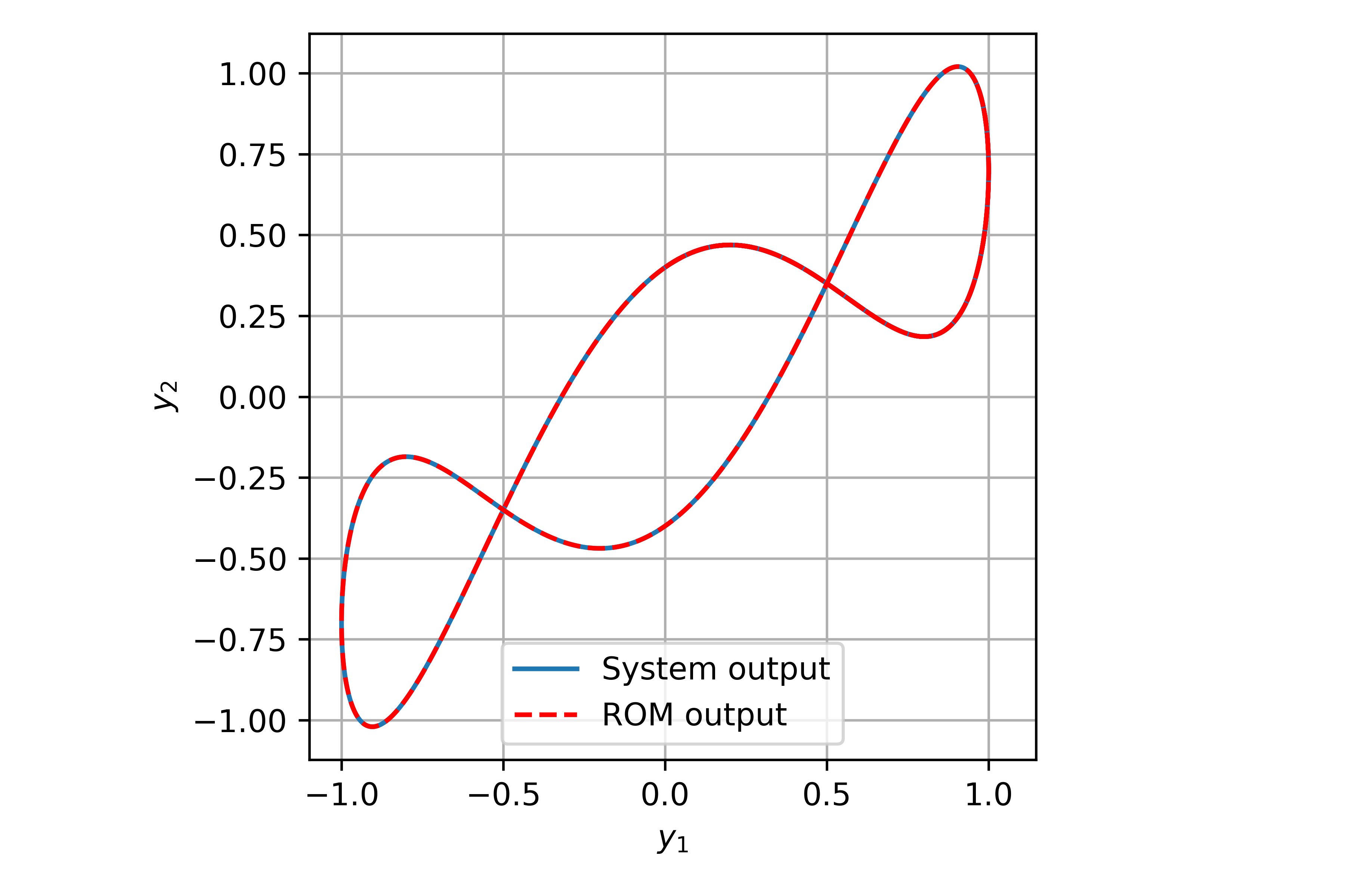
Figure 1: Original system and ROM outputs.

References

• Cardoso and Souloumiac (1996) Cardoso, J.F. and Souloumiac, A. (1996). Jacobi angles for simultaneous diagonalization. SIAM J. Mat. Anal. Appl., 17(1), 161–164.
• Cerjan et al. (2022) Cerjan, A., Loring, T.A., and Vides, F. (2022). Quadratic pseudospectrum for identifying localized states. 10.48550/ARXIV.2204.10450. URL https://arxiv.org/abs/2204.10450.
• De Moor (2019) De Moor, B. (2019). Least squares realization of lti models is an eigenvalue problem. In 2019 18th European Control Conference (ECC), 2270–2275. 10.23919/ECC.2019.8795987.
• Eynard et al. (2015) Eynard, D., Kovnatsky, A., Bronstein, M.M., Glashoff, K., and Bronstein, A.M. (2015). Multimodal manifold analysis by simultaneous diagonalization of laplacians. IEEE Transactions on Pattern Analysis and Machine Intelligence, 37(12), 2505–2517. 10.1109/TPAMI.2015.2408348.
• Loring (2015) Loring, T.A. (2015). $K$-theory and pseudospectra for topological insulators. Ann. Physics, 356, 383–416. 10.1016/j.aop.2015.02.031. URL http://dx.doi.org/10.1016/j.aop.2015.02.031.
• Vides (2021) Vides, F. (2021). Pytjae: A python toolset for truncated joint approximate eigenbases computation and reduced order modeling. URL https://github.com/FredyVides/PyTJAE.