Statistical and dynamical properties of quantum triangle map

Abstract

We study the statistical and dynamical properties of the quantum triangle map, whose classical counterpart can exhibit ergodic and mixing dynamics, but is never chaotic. Numerical results show that ergodicity is a sufficient condition for spectrum and eigenfunctions to follow the prediction of Random Matrix Theory, even though the underlying classical dynamics is not chaotic. On the other hand, dynamical quantities such as the out-of-time-ordered correlator (OTOC) and the number of harmonics, exhibit a growth rate vanishing in the semiclassical limit, in agreement with the fact that classical dynamics has zero Lyapunov exponent. Our finding show that, while spectral statistics can be used to detect ergodicity, OTOC and number of harmonics are diagnostics of chaos.

I Introduction

Classical ergodic theory provides a useful tool for the investigation of the statistical properties of classical dynamical systems with finite number of degrees of freedom. Indeed, the classical motion exhibits a rich variety of properties, ranging from complete integrability up to the exponential unstable chaotic motion, indistinguishable from a purely random process. The question if, and to what extent, this rich variety and beautiful complexity and intricacy of classical motion manifests itself in the quantum domain, has been the subject of quantum chaos. Here we refer the reader to the beautiful book of Fritz Haake [1], to whom this article is dedicated.

In other words: in the pure quantum context can we identify dynamical properties which play the same role as classical ergodic properties? In this connection a central role is played by the fact that the energy (or frequency) spectrum of any quantum system, bounded in phase space and with a finite number of degrees of freedom, is always discrete. This implies that the motion is quasi-periodic, which is just the opposite of classical chaotic motion which possesses a continuous frequency spectrum and exhibits statistical approach to equilibrium. On the other hand, the correspondence principle requires transition from quantum to classical mechanics for all phenomena, including dynamical chaos.

For a classical integrable system the energy spectrum can be obtained by semi-classical quantization rules. Instead for a classical chaotic system the complexity of the motion reflects in some statistical properties of the spectrum. In Ref [2], by considering a billiard in a stadium, it has been conjectured, and numerically verified, that the level spacing distribution of a classical chaotic systems is described by the celebrated Wigner-Dyson distribution od random matrix theory (RMT) which, in the statistical theory of spectra, has been introduced to describe the distribution of spectra of systems with many degrees of freedom [1]. Since these early times, the level statistics of classical chaotic systems has been studied in great detail, both theoretically and numerically, and we have now a quite satisfactory understanding [3, 4]. Yet we are very far from having a quantum ergodic hierarchy of statistical properties similar to the classical one.

For example, it is generally stated that the levels spacing distribution of chaotic systems is described by the Wigner-Dyson distribution. However, this statement is quite vague for at least two reasons:

(i) The level spacings distribution might depend on the energy range inside which the statistics is computed. Consider for example a prototype of chaotic systems: the stadium billiard. Classically, this system is chaotic no matter what energy and for any value of the parameter $\epsilon=a/r$, where $r$ is the radius of the circle and $a$ is length of the straight segment. However, if $\epsilon<<1$ the levels spacing distribution is not given by Wigner-Dyson up to energies which become larger and larger the smaller is $\epsilon$. The reason is due to the phenomenon of dynamical localization, which leads to the suppression of diffusion in angular momentum [5].

(ii) In the classical ergodic theory what is the minimal statistical property which leads to the Wigner-Dyson distribution of quantum level spacing statistics? Do we need mixing behaviour or is simple ergodicity sufficient?

In this paper, we address this question by considering the triangle map [6], which exhibits the same qualitative properties of triangular or polygonal billiards, but is much simpler for analytical and numerical investigations. The classical dynamics is not chaotic (even though it can become so in a generalized version of the map, discussed later in our paper, where the cusps in the potential are rounded-off) and, depending on the model parameters, is mixing, ergodic, quasi-ergodic [7], or quasi-integrable. Our results show that ergodicity is a sufficient condition to obtain spectral statistics as well as eigenfunction properties in agreement with RMT (see [9] for recent similar results for triangle billiards), while the quasi-ergodic case, where a single trajectory fills in the classical phase space extremely slowly in time [6], exhibits a different behavior depending on the quantity under scrutiny. That is, level spacing statistics is in good agreement with the Wigner-Dyson distribution in the semi-classical limit, while there exist eigenfunctions localized in phase space, incompatible with the predictions of RMT.

From our results it follows that level spacing statistics is unable to distinguish between chaotic and mixing or ergodic dynamics. For that purpose, we can consider the quantum dynamics in the time domain and study the out-of-time-ordered correlator (OTOC) [10, 11, 12, 13] or the number of harmonics of the phase-space Wigner distribution function [14, 15, 16, 17, 18, 19, 20, 21, 22]. Indeed, for chaotic dynamics the short-time behavior of both quantities exhibits an exponential increase at a rate which is determined by the largest Lyapunov exponent of the underlying classical dynamics [23, 24, 25]. Therefore, number of harmonics and OTOC can distinguish classically chaotic systems from those which are only mixing or ergodic. On the other hand, these quantities cannot distinguish between integrable and ergodic or mixing systems. For a rather complete picture of the manifestations of classical ergodic hierarchy on quantum systems one should therefore consider both spectral statistics and quantities in the time domain.

Our paper is organized as follows. in Sec. II, we introduce the classical and quantum triangle map, then we study the statistical properties of the quantum triangle map in Sec. III, while dynamical properties (OTOC and number of harmonics) are discussed in Sec. IV. Finally, conclusions and discussions are given in Sec. V.

II The triangle map

The classical triangle map [6] is defined on the torus with coordinates $(x,p)\in[-1,1)\times[-1,1)$ as follows:

$$\begin{cases}p_{n+1}=p_{n}-V^{\prime}(x_{n})&(\text{mod\,2}),\\ x_{n+1}=x_{n}+p_{n+1}&\text{(mod\,2)},\end{cases}$$ (1)

where $V(x)=-\alpha|x|-\beta x$. It is an area preserving, parabolic, piecewise linear map, which is related to a discrete bounce map for the billiard in a triangle. The map is marginally stable, i.e., initially close trajectories separate linearly with time. Even though the Lyapunov exponent is zero, numerical evidence indicates that this map can exhibit very different dynamics according to the parameters $\alpha$ and $\beta$. Specifically, we shall consider four cases: (i) $\alpha$ and $\beta$ are incommensurable irrational numbers: the map is ergodic and mixing; (ii) irrational $\beta$ and $\alpha=0$: the map is known to be ergodic but not mixing [26]; (iii) $\alpha$ is an irrational number and $\beta=0$: the system is quasi-ergodic (also referred to as weak ergodic [6], as extremely long times are required for a trajectory to fill in the phase space). (iv) the pseudo-integrable case with rational $\alpha$ and $\beta$; As shown by the Poincaré sections of Fig. 1 (drawn from a single orbit up to $T=10^{4}$ map steps), in the pseudo-integrable case only a finite number of values of $p$ appear, while in the ergodic and mixing cases a single orbit covers uniformly the surface. In the quasi-ergodic case, the number of different values of $p$ taken by a single orbit grows only logarithmically with the number $T$ of map iterations [6].

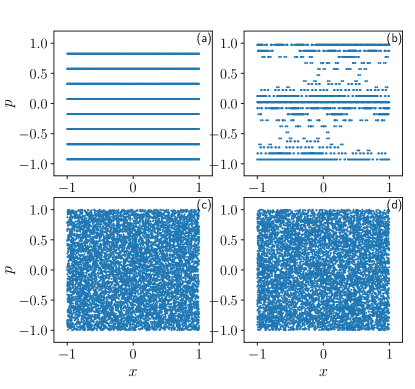
Figure 1: Poincaré sections for the classical triangle map drawn from a single orbit up to $T=10^{4}$ map iterations, for (a) pseudo-integrable case $\alpha=1/2,\ \beta=1/4$, (b) quasi-ergodic case $\alpha=(\frac{\sqrt{5}-1}{2}-e)/2,\ \beta=0$, (c) ergodic case $\alpha=0,\ \beta=(\frac{\sqrt{5}-1}{2}-e)/2$, (d) ergodic and mixing case, $\alpha=(\frac{\sqrt{5}-1}{2}-e)/2,\ \beta=(\frac{\sqrt{5}-1}{2}+e)/2$.

In the quantum case, the evolution over one map iteration is described by a (unitary) Floquet operator $U$ acting on the wave function $\psi$: $\psi_{n+1}=U\psi_{n}$, with

$$U=\exp\left(-i\frac{\hat{p}^{2}}{2\hbar}\right)\exp\left(-i\frac{V(\hat{x})}{\hbar}\right),$$ (2)

where $\hbar=\frac{2}{\pi D}$ is the effective Planck’s constant, $D$ being the Hilbert space dimension.

III Statistical properties

In this section, we study the statistical properties of the quantum triangle map. We consider the four different cases, corresponding to pseudo-integrable, quasi-ergodic, ergodic, and mixing behavior for the underlying classical triangle map. In Sect.III.1 we investigate the spectral statistics, focusing on the nearest neighbor spacing distribution, then in Sect.III.2 we study the distribution of the eigenfunctions’ components.

III.1 Spectral statistics

We study the standard indicator of quantum chaos, the nearest neighbor spacing distribution $P(s)$ of the eigenvalues of the Floquet operator $U$ of the triangle map.

First of all, we show in Fig. 2 the cumulative distribution $I(s)=\int_{0}^{s}ds^{\prime}\,P(s^{\prime})$, and compare it with the predictions of Random Matrix Theory, that is, with the cumulative distribution obtained from the Wigner-Dyson distribution of level spacings:

$$I_{W}(s)=1-\exp{(-\pi/4s^{2})}.$$ (3)

In order to see clearly the distance between $I(s)$ and $I_{W}(s)$, we also show (Fig. 3) $\ln(\ln(I(s)))$ as a function of $\ln(s)$.

Furthermore, to see how the distance between the level spacing distribution and the Wigner-Dyson distribution evolves approaching the classical limit, we also consider (see Fig. 4) the parameter $\langle r\rangle$ [27, 28] as a function of the effective Planck’s constant $\hbar$. The parameter $\langle r\rangle$ is obtained as mean value of $r_{k}$, defined as

$$r_{k}=\frac{\min({\Delta_{k},\Delta_{k+1}})}{\max{(\Delta_{k},\Delta_{k+1}})},$$ (4)

where $\Delta_{k}$ is the $k$-th level spacing of the spectrum of the Floquet operator. This parameter characterizes the correlations between adjacent gaps in the spectrum and RMT predicts $\langle r\rangle\approx 0.53$.

Our numerical simulations for all the above quantities show an excellent agreement with the predictions of RMT in the mixing case, and even in the ergodic but not mixing case. While the quantum chaos conjecture predicts statistical properties of classically chaotic quantum systems in agreement with the predictions of RMT, our results for a non-chaotic system suggest that the conjecture can be extended to a broader class of systems, with ergodicity as a sufficient condition for the onset of RMT behavior.

While the pseudo-integrable case clearly deviates from RMT predictions, the quasi-ergodic case is close to RMT, even though some differences are visible. On the other hand, data from Fig. 4 might suggest that spectral statistics approaches slowly the RMT predictions with decreasing $\hbar$, that is, when approaching the classical limit.

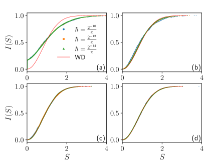
Figure 2: Cumulative distribution $I(s)$ of nearest level spacings for the triangle map, in the four cases (pseudo-integable, quasi-ergodic, ergodic, and mixing) of Fig. 1. The red solid line indicates the Wigner-Dyson cumulative distribution.

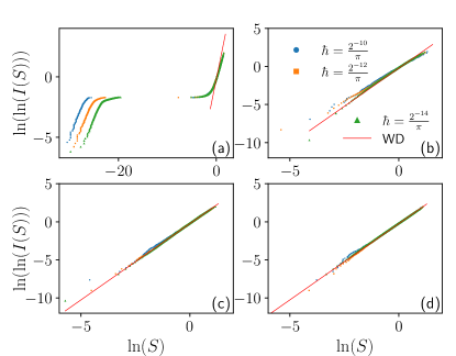
Figure 3: $\ln{(\ln{(I(s))})}$ versus $\ln{(s)}$ for four cases of Fig. 1. The red solid line indicates the Wigner-Dyson cumulative distribution.

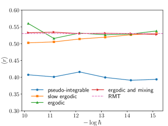
Figure 4: Parameter $\langle r\rangle$ for the four cases of Fig. 1. The dashed line indicates the RMT prediction $\langle r\rangle\approx 0.53$.

III.2 Eigenfunction of the Floquet operator

To further investigate the statistical properties of the triangle map, in this section we consider the distribution of the rescaled components (in the basis of the eigenstates of the operator $\hat{x}$, rescaled by $1/\sqrt{D}$) of each individual eigenfunction of the Floquet operator.

Since the triangle map is a time-reversal symmetric system, it is convenient to consider the symmetric Floquet operator

$$U_{\rm sym}=\exp\left(-i\frac{V(\hat{x})}{2\hbar}\right)\exp\left(-i\frac{\hat{p}^{2}}{2\hbar}\right)\exp\left(-i\frac{V(\hat{x})}{2\hbar}\right),$$ (5)

so that all the components of an eigenfunctions are real (up to an irrelevant global phase factor).

A first indicator of the agreement with the predictions of RMT for the components of an eigenfunction is the ratio between the second squared moment and the fourth moment of the components distribution:

$$\Lambda=\frac{({\cal M}_{2})^{2}}{{\cal M}_{4}}.$$ (6)

Note that RMT predict a Gaussian distribution of the components, for which $\Lambda=1/3$.

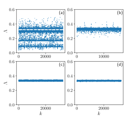
Figure 5: The ratio $\Lambda$ for every eigenstate ($k=1,...,D$, where $D=2^{15}$ is the Hilbert space dimension) in the triangle map for the four cases of Fig. 1 and $\hbar=\frac{2^{-14}}{\pi}$.

The value of the quantity $\Lambda$ for each individual state is shown in Fig.5, for $\hbar=\frac{2^{-14}}{\pi}$. On can see that both in the mixing and ergodic cases $\Lambda\simeq 1/3$ holds for almost all individual states. This result suggests, similarly to the above study of the spectral statistics, that ergodicity in the classical case is sufficient for the onset of RMT in the quantum case. The pseudo-integrable case is, as expected, incompatible with the RMT predictions. Finally, for the quasi-ergodic case most of the eigenstates have values $\Lambda\simeq 1/3$. On the other hand, there exist some localized states, with the value $\Lambda$ far from $1/3$. The Husimi function of the state with smallest value of $\Lambda$ is shown in Fig. 6(c): one can see that such state is indeed localized in phase space. The detailed distribution of rescaled components of some individual states are also shown in Fig. 6(a,b), where one can see that for “extended” states with $\Lambda\simeq 1/3$, the distribution indeed has a Gaussian shape, while for “localized” state, the distribution is far from being Gaussian.

It should be stressed here that the quasi-ergodic case is a little subtle in both classical [7] and quantum cases, and deserves further investigations to be clarified, which is beyond the scope of our current paper.

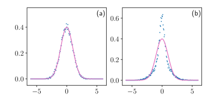
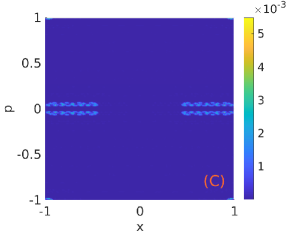
Figure 6: Distribution of rescaled components(rescaled by $1/\sqrt{D}$) of eigenfunctions, for both (a) “extended”($\Lambda\simeq 1/3$) and (b) “localized” (smallest value of $\Lambda$) states in the quasi-ergodic case $\alpha=(\frac{\sqrt{5}-1}{2}-e)/2,\ \beta=0$ and $\hbar=\frac{2^{-14}}{\pi}$.; (c) Husimi distribution for the localized state shown in (b).

IV Dynamical properties

The results of Sec. III show that spectral statistics can be used to detect ergodicity but not chaos in the semiclassical regime. For the latter purpose, one can investigate the short-time dynamics and use quantities such as the number of harmonics and the OTOC. As we shall discuss below, both quantities can measure the Lyapunov exponent, from their time-evolution within the Ehrenfest time scale.

IV.1 Out-of-time-ordered correlation

Here we consider the averaged OTOC, defined as

$$C_{L}(t)=\frac{1}{N}\sum_{k=1}^{N}\ln\left(\langle\psi_{k}|[\hat{x}(t),\hat{p}(0)]^{2}|\psi_{k}\rangle\right).$$ (7)

The average is taken over a large number $N$ of initial coherent states,

$$\psi_{k}(x)=(\pi\hbar)^{-1/4}\exp\left(-\frac{(x-x_{k})^{2}}{2\hbar}+\frac{ip_{k}x}{\hbar}\right),$$ (8)

with $(x_{k},p_{k})$ is the center of the $k$-th initial state, randomly distributed in the phase space. The classical correspondence of $C_{L}(t)$, denoted as $C_{L}^{\rm cl}(t)$, is obtained by the canonical substitution $\frac{1}{i\hbar}[\hat{A},\hat{B}]\rightarrow\{A,B\}_{\text{PB}}$, where the right-hand side is the Poisson bracket of the classical variables $A$ and $B$. We can write the classical counterpart of the OTOC as

$$C_{L}^{\rm cl}(t)=\frac{1}{N}\sum_{k=1}^{N}\ln\left[\int d\boldsymbol{\gamma}\rho_{\boldsymbol{\gamma}_{0}^{k}}(\boldsymbol{\gamma})\left(\frac{\partial x(t)}{\partial x(0)}\right)^{2}\right],$$ (9)

where $\gamma=(x,p)$. The initial condition is a Gaussian distribution

$$\rho_{\boldsymbol{\gamma_{0}^{k}}}(\boldsymbol{\gamma})=(2\pi\sigma^{2})^{-1}\exp\left(-\frac{(x-x_{k})^{2}+(p-p_{k})^{2}}{2\sigma^{2}}\right),$$ (10)

where, in order to compare with the quantum wavepacket, we take $\sigma=\sqrt{\frac{\hbar}{2}}$.

Note that we take the average of the logarithms of the OTOC of the individual initial states $\psi_{k}$. The simple average, instead, would lead to a divergence since there are singular points (the cusps in the potential) for which $\partial x(t)/\partial x(0)$ diverges. This is a general problems when taking the simple average of OTOCs [29, 30, 31], as it is dominated in integrable systems by the local instability of unstable fixed points, which might lead to an exponential growth completely unrelated to chaos. On the other hand, as we shown in Ref. [25], a proper averaging (of the logarithms of OTOC) restores the role of OTOC as a diagnostic of chaotic dynamics, as

$$C_{L}(t)\propto 2\lambda t,$$ (11)

where $\lambda$ is the largest Lyapunov exponent of the underlying dynamics, and this growth lasts up to the Ehrenfest time scale. Therefore, we expect a linear in time growth of $C_{L}(t)$ for chaotic dynamics, with the growth rate measuring the “quantum Lyapunov” exponent.

It can be seen from Fig. 7 that, for all the cases above considered (pseudo-integrable, quasi-ergodic, ergodic, and mixing), $C_{L}(t)$ behaves similarly. That is, for $\hbar\to 0$ the growth rate vanishes, indicating a zero “quantum Lyapunov” exponent in the semiclassical limit.

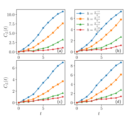
Figure 7: The averaged OTOC $C_{L}(t)$ in triangle map for the four different cases of Fig. 1.

IV.2 Number of harmonics

For classical chaotic dynamics, the exponential sensitivity implies that the density distribution in the phase space is exponentially stretched and folded, becoming increasingly intricate on smaller and smaller scales. Therefore, in order to reconstruct the increasingly finer details of the phase-space distribution, the number of harmonics, that is, components in Fourier space, also increases exponentially in time [15, 17, 18]. In an integrable system this does not happen, as the instability is typically linear in time [32]. It follows that the growth rate of the number of harmonics of the phase-space distribution can be used, similarly to the Lyapunov exponent, as a way to characterize classical chaos. The advantage is that this phase space approach, in contrast with the exponential instability of trajectories, can be transferred to the quantum domain.

Indeed, we consider the Fourier transform of the Wigner function $W(x,p)$:

$$W(x,p)=\sum_{m,n}\tilde{W}_{m,n}e^{-i\pi(mx+np)}.$$ (12)

The number of harmonics is then estimated from the square root of the second moment ${\cal M}_{2}$ of the harmonics distribution:

$${\cal M}_{2}=\sum_{m,n}(m^{2}+n^{2})\tilde{W}_{m,n}.$$ (13)

For pure initial states, we obtain [18]

$${\cal M}_{2}=\frac{2}{\hbar^{2}}\,(\Delta_{2}(\hat{x})+\Delta_{2}(\hat{p})),$$ (14)

where

$$\Delta_{2}(x)=\langle\hat{x}^{2}\rangle-\langle\hat{x}\rangle^{2},\quad\Delta_{2}(p)=\langle\hat{p}^{2}\rangle-\langle\hat{p}\rangle^{2}.$$ (15)

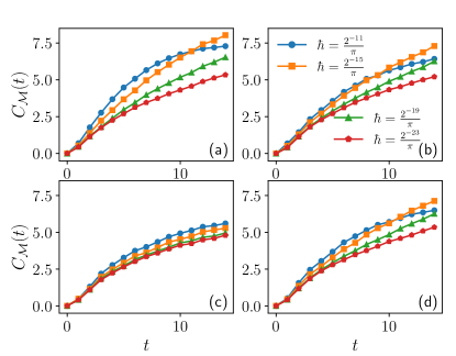
Figure 8: The averaged number of harmonics $C_{\cal M}(t)$ in triangle map for the four different cases of Fig. 1.

We then average the logarithms of the second moment ${\cal M}_{2}^{(k)}(t)$ for the initial states $\{\psi_{k}\}$:

$$C_{{\cal M}}(t)=\frac{1}{N}\sum_{k=1}^{N}\ln\left({\cal M}_{2}^{(k)}(t)\right),$$ (16)

where the average is performed as in the case of OTOC.

The numerical results, shown in Fig. 8, confirm the main message obtained from the study of the OTOC. We cannot find an $\hbar$-independent growth rate for the number of harmonics, in all the considered cases (pseudo-integrable, quasi-ergodic, ergodic, and mixing). These results should be contrasted with those of the chaotic case, where a growth rate given by twice the Lyapunov exponent is observed (see discussion in Sec. IV.3 and the data shown in Fig. 9).

IV.3 Comparison with chaotic case

We compare the results obtained so far with those for a chaotic system. We consider a round-off triangle map [25], in which we substitute the cusps in the potential $V(x)$ of the original triangle map by small circle arcs of radius $r$:

$$\frac{V(x)}{\alpha}=\begin{cases}-\sqrt{2}r+\sqrt{r^{2}-x^{2}}&|x|\leq\frac{\sqrt{2}}{2}r,\\ -1+\sqrt{2}r-\sqrt{r^{2}-(|x|-1)^{2}}&|x|\geq 1-\frac{\sqrt{2}}{2}r,\\ -|x|&{\rm otherwise}.\end{cases}$$ (17)

Differently from the original triangle map (recovered for $r=0$), the round-off triangle map is exponentially unstable for any $r\neq 0$, that is, the maximum Lyapunov exponent is positive. In Fig. 9, we show OTOC and number of harmonics for $r=0.2$. One can see that for both quantities the initial growth follows, up to the Ehrenfest time, a slope given by twice the Lyapunov exponent of the classical chaotic dynamics. Therefore, OTOC and number of harmonics can be used to detect and quantify exponential instability in the semi-classical limit $\hbar\rightarrow 0$. This is not possible using spectral statistics, which follows Random Matrix Theory for chaotic but also for non-chaotic, mixing or even uniquely ergodic systems.

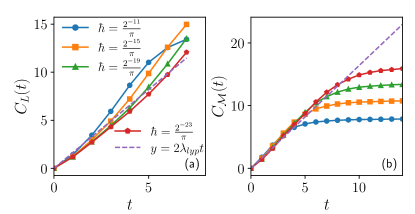
Figure 9: The averaged OTOC $C_{L}(t)$ and the averaged number of harmonics $C_{\cal M}(t)$ in the round-off triangle map for $r=0.2$, $\alpha=(\frac{\sqrt{5}-1}{2}-e)/2,\ \beta=0$. Note the sharp contrast between this figure and Figs. 7 and 8: in those figures the growth rate decreases with $\hbar$, while here it is $\hbar$-independent.

V Conclusions and Discussions

By studying the statistical properties of different cases of the quantum triangle map, we find that ergodicity is a sufficient condition for the onset of random matrix behavior, in the properties of both spectrum and eigenfunctions. Therefore, to detect classically chaotic motion in a quantum system, one should rather consider quantities in the time domain, such as the OTOC and the number of harmonics, whose growth rate is determined by the classical Lyapunov exponent. While such quantities are sensitive indicators of classical chaotic dynamics, in order to distinguish between integrable and ergodic or mixing dynamics one should instead use spectral statistics. Given the quantities discussed in this paper, the problem remains to distinguish between mixing and uniquely ergodic dynamics. This problem could be tackled by looking at the decay of correlation functions, as done for the classical triangle map [6].

Acknowledgments: J. Wang acknowledges the financial support of the Deutsche Forschungsgemeinschaft (DFG), Grants No. 397107022 (GE 1657/3-2) and No. 397067869 (STE 2243/3-2) within the DFG Research Unit FOR 2692. G.B. acknowledges the financial support of the INFN through the project “QUANTUM”. W.-g. Wang acknowledges the financial support of the Natural Science Foundation of China under Grant Nos. 11535011, 11775210, and 12175222.

References

- [1] F. Haake, S. Gnutzmann, and M. Kuś, Quantum Signatures of Chaos (4th ed.) (Springer, 2018).
- [2] G. Casati, F. Valz-Gris, and I. Guarneri, Lettere al Nuovo Cimento 28, 279 (1980).
- [3] O. Bohigas, M.-J. Giannoni, and C. Schmit, Phys. Rev. Lett. 52, 1 (1984). In this paper, the model studied in Ref [2] was investigated in a more complete and clear fashion and the conjecture in [2] confirmed.
- [4] T. Guhr, A. Müller-Groeling, H.A. Weidenmüller, Phys. Rep. 299, 189 (1998).
- [5] F. Borgonovi, G. Casati, and B. Li, Phys. Rev. Lett. 77, 4744 (1996).
- [6] G. Casati and T. Prosen, Phys. Rev. Lett. 85, 4261 (2000).
- [7] Quasi-ergodicity is a weaker property than ergodicity. Indeed, for quasi-ergodic systems one cannot prove that time averages are equal to phase averages. For instance, for the system of two elastic hard-point masses in one dimension with generic mass ratio, numerical results indicate that the orbits are dense on the energy surface, yet the system is nonergodic [8]. It is an open problem whether the triangle map in the quasi-ergodic regime can exhibit the same phenomenon.
- [8] J. Wang, G. Casati, and T. Prosen, Phys. Rev. E 89, 042918 (2014).
- [9] C. Lozej, G. Casati, and T. Prosen, preprint arXiv:2110.04168 [nlin.CD].
- [10] A. Larkin and Y. N. Ovchinnikov, Zh. Eksp. Teor. Fiz. Sov. Phys. 55, 1200 (1968) [JETP 28, 1200 (1969)].
- [11] A. Kitaev, Hidden correlations in the Hawking radiation and thermal noise, talk given at KITP, Santa Barbara, 2014, http://online.kitp.ucsb.edu/online/joint98/kitaev/.
- [12] J. Maldacena and D. Stanford, Phys. Rev. D 94, 106002 (2016).
- [13] J. Maldacena, S. H. Shenker, and D. Stanford, J. High Energy Phys. 08 (2016) 106.
- [14] B. V. Chirikov, F. M. Izrailev, and D. L. Shepelyansky, Sov. Sci. Rev. C 2, 209 (1981).
- [15] Y. Gu, Phys. Lett. A 149, 95 (1990).
- [16] Y. Gu and J. Wang, Phys. Lett. A 229, 208 (1997).
- [17] A. K. Pattanayak and P. Brumer, Phys. Rev. E 56, 5174 (1997).
- [18] J. Gong and P. Brumer, Phys. Rev. A 68, 062103 (2003).
- [19] V. V. Sokolov, O. V. Zhirov, G. Benenti, G. Casati, Phys. Rev. E 78, 046212 (2008).
- [20] G. Benenti and G. Casati, Phys. Rev. E 79, 025201 (R) (2009).
- [21] V. Balachandran, G. Benenti, G. Casati, and J. Gong, Phys. Rev. E 82, 046216 (2010).
- [22] P. Qin, W. Wang, G. Benenti, and G. Casati, Phys. Rev. E 89, 032120 (2014).
- [23] E. B. Rozenbaum, S. Ganeshan, and V. Galitski, Phys. Rev. Lett. 118, 086801 (2017).
- [24] J. Wang, G. Benenti, G. Casati, and W. Wang, Phys. Rev. Res. 2, 043178 (2020).
- [25] J. Wang, G. Benenti, G. Casati and W. Wang, Phys. Rev. E 103, L030201 (2021).
- [26] H. Furstenberg, Am. J. Math. 83, 573 (1961).
- [27] V. Oganesyan and D. A. Huse, Phys. Rev. B 75, 155111 (2007).
- [28] Y. Y. Atas, E. Bogomolny, O. Giraud, and G. Roux Phys. Rev. Lett. 110, 084101 (2013).
- [29] S. Pilatowsky-Cameo, J. Chávez-Carlos, M. A. Bastarrachea-Magnani, P. Stránský, S. Lerma-Hernández, L. F. Santos, and J. G. Hirsch, Phys. Rev. E 101, 010202 (2020).
- [30] T. Xu, T. Scaffidi, and X. Cao, Phys. Rev. Lett. 124, 140602 (2020).
- [31] E. B. Rozenbaum, L. A. Bunimovich, and V. Galitski, Phys. Rev. Lett. 125, 014101 (2020).
- [32] G. Casati, J. Ford, and B. V. Chirikov, Phys. Lett. 77A, 91 (1980).