Abstract

We study here the escape time for the fastest diffusing particle from the boundary of an interval with point-sink killing sources. Killing represents a degradation that leads to the probabilistic removal of the moving Brownian particles. We compute asymptotically the mean time it takes for the fastest particle escaping alive and obtain the extreme statistic distribution. These computations relies on an explicit expression for the time dependent flux of the Fokker-Planck equation using the time dependent Green’s function and Duhamel’s formula. We obtain a general formula for several point-sink killing, showing how they directly interact. The range of validity of the present formula for the mean extreme times of the fastest is evaluated with Brownian simulations. Finally, we discuss some applications to the early calcium signaling at neuronal synapses.

Extreme diffusion with point-sink killing fields for fast calcium signaling at synapses
S. Toste¹ D. Holcman ²

60G70, 35K05, 60J70, 92-10

1 Introduction

For more than a century, the time scale of molecular activation has relied on the Smoluchowski’s computation for the flux of a single particle reaching an absorbing sphere, a process modeled by the associated diffusion equation [7, 41, 11, 37]. This flux defines the reciprocal of the forward binding rate and also the time scale of cellular activation with a single molecular event. However, recently the time scale of activation for signaling event associated with calcium transients at neuronal synapses was found to be much faster than the one predicted by Smoluchowski’s rate. This paradox about the fast time scale can be explained by the extreme statistical events [39] for the arrival time of the fastest particles among many [2, 5, 3]. Briefly, there is no need of transporting a distribution of particles from one region to another to generate a response: the fastest arriving particles are sufficient to trigger the needed events after finding and binding to the key narrow targets. This event can for example open a channel that can trigger the release of the same species. This is well known in the case of calcium, known as calcium-induce-calcium-release [9]. The time of the fastest to arrive to a small target is in fact modulated by the initial copy number of identically distributed random particles. Recently, we hypothesize that this number sets the time to activation in most signaling molecular events, reproduction, gene expression and it is thus a fundamental achievement of life evolution at mostly all levels [40, 8, 31, 34, 35, 38, 44, 45, 29]. Such large number guarantees that a rare event that would be impossible to trigger in a reasonable time scale will actually take place by the fastest particles in a reasonable time. This large number compensates for the unknown position of the small targets and the hidden geometry to be explored. The initial distribution of particles is often well separated from these target. This large number has been well calibrated for each applications, summarized as the redundancy principle [40].
The extreme statistics theory allows to compute the mean time of the fastest with respect to the parameters of the problem such as the diffusion coefficient for a diffusion process, the distance to the source and the initial number of particle [47, 48, 51]. The computations have been extended to sub- and super- diffusion, but also when the initial distribution can extend close to the target window [12, 23, 24, 46, 27].
In the present manuscript, we study the role of a killing source that can terminate the trajectory of a random particle before it can reach a target. The killing measure is the probability per unit time and unit length to terminate a trajectory. However, a moving particle can pass through a killing site many times without being terminated, in contrast to an absorbing boundary, where the trajectory is terminated with probability 1. Such a killing event can modify the escape time, due to the probability to be killed before escape [14]. The probability of reaching small target and the conditional mean times are relevant to quantify the success of viral infection in cells [22] or spermatozoa in the uterus [36, 33, 49].

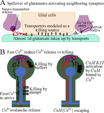
Figure 1: Escape versus killing in the regulation of molecular neuronal signaling. A. Spillover of neurotransmitters after synaptic activation between glial cells (yellow), that contain transporters (modeled as killing term) to remove them from the extra-cellular space. Trajectory can be terminated (red) or arrive to receptor to activate the influx of ion in the neighboring synaptic terminal (purple).B. Left: Calcium dynamics in a dendritic spine: the fastest calcium ions can trigger a process called calcium-induce-calcium-release, if the ions are not stopped by a long-time binding buffer or extruded by pumps. Right: CaMKII kinase activation by calcium bound to calmodulin molecules. The probability and the mean time to activate the kinase CaMKII by the first calmodulin bound to calcium is one of the application explained here.

We are interesting here, in computing the mean time it takes for the fastest among many independent and equally distributed Brownian particles to reach a target when the killing measure is a sum of Dirac-delta functions located in an interval. To illustrate the present approach and the relevant of dimension reduction, we shall use two examples from neuroscience: the first one concerns the spillover of neurotransmitters such glutamate after synaptic activation. The neurotransmitters diffuse near glial cells that contains transporters (Fig. 1A), the role of which is to remove these neurotransmitters from the extra-cellular space. This extrusion mechanism can be modelled as a one dimensional process with killing in an interval due the small space separation along the thin axone or dendrite. The second example concerns calcium dynamics in dendritic spines: the fastest calcium ions that enter following synaptic activation can trigger fast calcium release. However the fastest calcium ions should be interrupted by long-time binding buffers or extruded by pumps on their way to the base of the spine (Fig. 1B). This interruption mechanism can be modeled by a killing term. We will also discuss below the case of calcium bound to calmodulin that can activate the CaMKII kinase. We propose to compute the probability and the mean time to activate a CaMKII [25]. This activation is relevant for the induction of long-term memory at a synaptic level. Here the relevant time is the first time that one CaM containing two calcium ions will arrive at a CAMKII before it exits. This process is computed as the first bound to CaMKII, modeled by a killing measure.
In these examples, the role of the killing term is to terminate the particle trajectories at random times. The effect of the killing measure is accounted by an additive term in the Fokker-Planck equation, that describes the probability density function of the survival process before escape [19, 20, 6, 14, 32].
The manuscript is organized as follows: in Section 2, we summarize the background: stochastic formulation and Fokker-Planck equation relevant to compute the mean first escape time under a killing field [16]. In Section 3, using a short-time asymptotic expansion of the diffusion equation with a single and multiples Dirac-delta killing measures, we derive a formula for the mean escape time for the first among many trajectories to escape before being killed in half-a-line. In Section 4, we discuss the asymptotic result with respect to the stochastic simulations. In Section 4.2, we apply the present concept to model and determine the time of key calcium activation processes that can trigger long-term memory in dendritic spines.

2 General background: killing measure versus survival probability

2.1 Stochastic framework

A stochastic process $\mbox{\boldmath$x$}(t)$ in the domain $\Omega$ satisfies the equation

(1) $$d{\mbox{\boldmath$x$}}=\mbox{\boldmath$b$}(\mbox{\boldmath$x$})\,dt+\sqrt{2}\mbox{\boldmath$B$}(\mbox{\boldmath$x$})\,d{\mbox{\boldmath$w$}}(t)\hskip 5.0pt,\mbox{for}\ \mbox{\boldmath$x$}\in\Omega,$$

where $\mbox{\boldmath$b$}(\mbox{\boldmath$x$})$ is a smooth drift vector, $\mbox{\boldmath$B$}(\mbox{\boldmath$x$})$ is a diffusion tensor, and $\mbox{\boldmath$w$}(t)$ is a vector of independent standard Brownian motions. A killing measure $k(\mbox{\boldmath$x$})$ is added in the domain $\Omega$ with boundary $\partial\Omega=\partial\Omega_{a}\cup\partial\Omega_{r}$, where $\partial\Omega_{a}$ is a small absorbing part and $\partial\Omega_{r}$ is the reflecting boundary. The transition probability density function (pdf) of the process $\mbox{\boldmath$x$}(t)$ with killing and absorption is the pdf of trajectories that have neither been killed nor absorbed in $\partial\Omega_{a}$ by time $t$,

$$p(\mbox{\boldmath$x$},t\,|\,\mbox{\boldmath$y$})\,d\mbox{\boldmath$x$}=\Pr\{\mbox{\boldmath$x$}(t)\in\mbox{\boldmath$x$}+d\mbox{\boldmath$x$},\,\tau^{k}>t,\,\tau^{e}>t\,|\,\mbox{\boldmath$y$}\},$$

where $\tau^{k}$ is the time for the particle to be killed and $\tau^{e}$ is the time of absorbtion. This pdf is the solution of the Fokker-Planck equation (FPE) [41]

(2) $$\frac{\partial p(\mbox{\boldmath$x$},t\,|\,\mbox{\boldmath$y$})}{\partial t}={\cal L}_{\mbox{\boldmath$x$}}p(\mbox{\boldmath$x$},t\,|\,\mbox{\boldmath$y$})-k(\mbox{\boldmath$x$})p(\mbox{\boldmath$x$},t\,|\,\mbox{\boldmath$y$})\hskip 5.0pt\ \mbox{for}\ \mbox{\boldmath$x$},\mbox{\boldmath$y$}\in\Omega,$$

where ${\cal L}_{\mbox{\boldmath$x$}}$ is the forward operator

(3) $${\cal L}_{\mbox{\boldmath$x$}}p(\mbox{\boldmath$x$},t\,|\,\mbox{\boldmath$y$})=\sum_{i,j=1}^{d}\frac{\partial^{2}\sigma^{i,j}(\mbox{\boldmath$x$})p(\mbox{\boldmath$x$},t\,|\,\mbox{\boldmath$y$})}{\partial x^{i}\partial x^{j}}-\sum_{i=1}^{d}\frac{\partial b^{i}(\mbox{\boldmath$x$})p(\mbox{\boldmath$x$},t\,|\,\mbox{\boldmath$y$})}{\partial x^{i}},$$

and $\mbox{\boldmath$\sigma$}(\mbox{\boldmath$x$})=\frac{1}{2}\mbox{\boldmath$B$}(\mbox{\boldmath$x$})\mbox{\boldmath$B$}^{T}(\mbox{\boldmath$x$})$. The operator ${\cal L}_{\mbox{\boldmath$x$}}$ can be written in the divergence form ${\cal L}_{\mbox{\boldmath$x$}}p(\mbox{\boldmath$x$},t\,|\,\mbox{\boldmath$y$})=-\nabla\cdot\mbox{\boldmath$J$}(\mbox{\boldmath$x$},t\,|\,\mbox{\boldmath$y$})$, where the components of the flux density vector $\mbox{\boldmath$J$}(\mbox{\boldmath$x$},t\,|\,\mbox{\boldmath$y$})$ are

$$J^{i}(\mbox{\boldmath$x$},t\,|\,\mbox{\boldmath$y$})=-\sum_{j=1}^{d}\frac{\partial\sigma^{i,j}(\mbox{\boldmath$x$})p(\mbox{\boldmath$x$},t\,|\,\mbox{\boldmath$y$})}{\partial x^{i}}+b^{i}(\mbox{\boldmath$x$})p(\mbox{\boldmath$x$},t\,|\,\mbox{\boldmath$y$}),\hskip 5.0pt(i=1,2,\ldots,d).$$

The initial and boundary conditions for the FPE (2) are

$$p(\mbox{\boldmath$x$},0\,|\,\mbox{\boldmath$y$}) = \,\delta(\mbox{\boldmath$x$}-\mbox{\boldmath$y$})\hskip 5.0pt\mbox{for}\ \mbox{\boldmath$x$},\mbox{\boldmath$y$}\in\Omega$$

$$p(\mbox{\boldmath$x$},t\,|\,\mbox{\boldmath$y$}) = \,0\hskip 5.0pt\mbox{for}\ t>0,\ \mbox{\boldmath$x$}\in\partial\Omega_{a},\ \mbox{\boldmath$y$}\in\Omega$$

$$\mbox{\boldmath$J$}(\mbox{\boldmath$x$},t\,|\,\mbox{\boldmath$y$})\cdot\mbox{\boldmath$n$}(\mbox{\boldmath$x$}) = \,0\hskip 5.0pt\mbox{for}\ t>0,\ \mbox{\boldmath$x$}\in\partial\Omega-\partial\Omega_{a},\ \mbox{\boldmath$y$}\in\Omega.$$

The particular case where there is no drift vector, this is $b(x)=0$, the FPE with the initial and boundary conditions written as above models the diffusive Brownian motion of particles that start at point $y$. These particles are absorbed at point $x=0$ or degraded by the killing measure $k(\mbox{\boldmath$x$})$.
The probability of trajectories that are killed before reaching $\partial\Omega_{a}$ is given by [17],

$$\Pr\{\tau^{k}<\tau^{e}\,|\,\mbox{\boldmath$y$}\}=\int\limits_{0}^{\infty}\int\limits_{\Omega}k(\mbox{\boldmath$x$})p(\mbox{\boldmath$x$},t\,|\,\mbox{\boldmath$y$})\,d\mbox{\boldmath$x$}\,dt.$$

The absorption probability flux on $\partial\Omega_{a}$ is

(4) $$J(t\,|\,\mbox{\boldmath$y$})=\oint_{\partial\Omega}\mbox{\boldmath$J$}(\mbox{\boldmath$x$},t\,|\,\mbox{\boldmath$y$})\cdot\mbox{\boldmath$n$}(\mbox{\boldmath$x$})\,dS_{\mbox{\boldmath$x$}},$$

and $\int_{0}^{\infty}J(t\,|\,\mbox{\boldmath$y$})\,dt$ is the probability of trajectories that have been absorbed at $\partial\Omega_{a}$. Thus the probability to escape before being killed is

(5) $$\Pr\{\tau^{e}<\tau^{k}\,|\,\mbox{\boldmath$y$}\}=\int_{0}^{\infty}J(t\,|\,\mbox{\boldmath$y$})\,dt.$$

The pdf of the killing time $\tau^{k}$ is the conditional probability of killing before time $t$ of trajectories that have not been absorbed in $\partial\Omega_{a}$ by that time

$$\Pr\{\tau^{k}<t\,|\,\tau^{e}>\tau^{k},\mbox{\boldmath$y$}\}=\frac{\Pr\{\tau^{k}<t,\tau^{e}>\tau^{k}\,|\,\mbox{\boldmath$y$}\}}{\Pr\{\tau^{e}>\tau^{k}\,|\,\mbox{\boldmath$y$}\}}=\frac{\displaystyle{\int}_{0}^{t}\int_{\Omega}k(\mbox{\boldmath$x$})p(\mbox{\boldmath$x$},s\,|\,\mbox{\boldmath$y$})\,d\mbox{\boldmath$x$}\,ds}{\displaystyle{\int}_{0}^{\infty}\int_{\Omega}k(\mbox{\boldmath$x$})p(\mbox{\boldmath$x$},s\,|\,\mbox{\boldmath$y$})\,d\mbox{\boldmath$x$}\,ds}.$$

The probability distribution of the time to absorption at $\partial\Omega_{a}$ is the conditional probability of absorption before time $t$ of trajectories that have not been killed by that time

$$\Pr\{\tau^{e}<t\,|\,\tau^{k}>\tau^{e},\mbox{\boldmath$y$}\}=\frac{\displaystyle{\int}_{0}^{t}J(s\,|\,\mbox{\boldmath$y$})\,ds}{1-\displaystyle{\int}_{0}^{\infty}\int_{\Omega}k(\mbox{\boldmath$x$})p(\mbox{\boldmath$x$},s\,|\,\mbox{\boldmath$y$})\,d\mbox{\boldmath$x$}\,ds}.$$

Thus the narrow escape time (NET) is the conditional expectation of the absorption time of trajectories that are not killed in $\Omega$, that is,

$$\mathbb{E}[\tau^{e}\,|\,\tau^{k}>\tau^{e},\,\mbox{\boldmath$y$}]=\,\int\limits_{0}^{\infty}\Pr\{\tau^{e}>t\,|\,\tau^{k}>\tau^{e},\mbox{\boldmath$y$}\}\,dt=\,\frac{\displaystyle{\int}_{0}^{\infty}sJ(s\,|\,\mbox{\boldmath$y$})\,ds}{1-\displaystyle{\int}_{0}^{\infty}\int_{\Omega}k(\mbox{\boldmath$x$})p(\mbox{\boldmath$x$},s\,|\,\mbox{\boldmath$y$})\,d\mbox{\boldmath$x$}\,ds}.$$

The survival probability of trajectories that have not been terminated by time $t$ is given by

(6) $$S(t\,|\,\mbox{\boldmath$y$})=\int\limits_{\Omega}p(\mbox{\boldmath$x$},t\,|\,\mbox{\boldmath$y$})\,d\mbox{\boldmath$x$}.$$

For specific assumptions about the geometry of $\Omega$ and the distribution of absorbing windows, we refer to [17].

2.2 Extreme escape statistics with killing

For $N_{0}$ independent identically distributed copies of the stochastic process (1), that can escape at time $t_{1},...,t_{N_{0}}$, prior to get killed, we consider the escape time of the fastest one and we shall derive here a formula for the probability and mean escape time of the fastest Brownian motion. The extreme mean first passage time (EMFPT) $\bar{\tau}_{\footnotesize\mbox{EMFPT}}(n)$ [21, 17] is the fastest time for a particle to escape through one of a narrow window located on the surface of the domain $\Omega$, that is

$$\tau_{\footnotesize\mbox{EMFPT}}(n)=\underset{n}{\min}\{t_{1},...,t_{n}\}.$$

All these times are conditioned to the fact that at least a large number of particles have to escape, so that $n\gg 1$ and $n\leq N_{0}$, where $n$ is the number of survival particles. The conditional mean first passage time (MFPT) ${\bar{\tau}}^{j}_{n}$ of the $j^{th}$ particle serves to compute $\tau_{EMFPT}(n)$ of the first particle that has reached the absorbing boundary $\partial\Omega_{a}$.
The pdf of the escape time of the first particle prior to time $t$ with an initial density $p_{0}(x)$ is given by

$$P(t)=\Pr\{\tau^{e}_{EMFPT}(n)<t\,|\,\tau^{e}_{EMFPT}(n)<\tau^{k}_{EMFPT}(n),p_{0}\}.$$

The conditional MFPT $\bar{\tau}_{EMFPT}(n)$ is defined by

(7) $$\bar{\tau}_{EMFPT}(n)=\int\limits_{0}^{\infty}t\frac{dP(t)}{dt}\,dt=\int\limits_{0}^{\infty}\left[P(\infty)-P(t)\right]\,dt.$$

Using Bayes’ law, we obtain the decomposition

(8) $$P(t)=\frac{\Pr\{\tau^{e}_{EMFPT}(n)<t,\tau^{e}_{EMFPT}(n)<\tau^{k}_{EMFPT}(n),p_{0}\}}{\Pr\{\tau^{e}_{EMFPT}(n)<\tau^{k}_{EMFPT}(n),p_{0}\}}=\frac{N(t)}{P_{\infty}},$$

where $P_{\infty}$ is the probability that the fastest one escape and the numerator $N(t)$ is defined as the conditional probability that the fastest one escapes alive before time $t$. Then, the extreme mean first passage time is conditioned to that at least one particle has to escape ($n\geq 1$).

2.2.1 Probability that the fastest particle escapes

The probability that the fastest particle escapes alive the domain is computed as follows

$$P_{\infty}=\Pr\{\tau^{e}_{EMFPT}(n)<\tau^{k}_{EMFPT}(n),p_{0}\}=1-\Pr\{\tau^{e}_{EMFPT}(n)>\tau^{k}_{EMFPT}(n),p_{0}\}.$$

Using that particles are independent, we get

$$P_{\infty}=1-\prod_{j=1}^{n}\Pr\{\tau^{e}_{j}>\tau^{k}_{j},p_{0}\},$$

which can be written as

$$P_{\infty}=1-\left(1-\Pr\{\tau^{e}<\tau^{k},p_{0}\}\right)^{n}.$$

According to relation (5), because the probability that a single particle escapes before being killed is given by $\Pr\{\tau^{e}<\tau^{k},p_{0}\}=\int_{0}^{\infty}\int_{\mbox{\boldmath$y$}\in\Omega}J(t\,|\,\mbox{\boldmath$y$})p_{0}(\mbox{\boldmath$y$})d\mbox{\boldmath$y$}\,dt$ then,

$$P_{\infty}=1-\left(1-\int_{0}^{\infty}\int_{\mbox{\boldmath$y$}\in\Omega}J(t\,|\,\mbox{\boldmath$y$})p_{0}(\mbox{\boldmath$y$})d\mbox{\boldmath$y$}\,dt\right)^{n}.$$

For a Dirac-delta initial distribution at position $y$, we get

(9) $$P_{\infty}=1-\left(1-\int_{0}^{\infty}J(t\,|\,\mbox{\boldmath$y$})dt\right)^{n},$$

where the flux $J$ is given by relation (4). Finally, the probability that $n-k$ particles are killed and only $k$ escape alive is given by the Binomial distribution

$$\Pr\{\tau^{k}<\tau^{e},\tau^{q}>\tau^{e},q=k+1,\ldots,n\}=\binom{n}{k}\left(\int_{0}^{\infty}J(t\,|\,\mbox{\boldmath$y$})dt\right)^{k}\left(1-\int_{0}^{\infty}J(t\,|\,\mbox{\boldmath$y$})dt\right)^{n-k}.$$

2.3 Mean time for the fastest to escape without being killed

The conditional probability that the fastest one escapes alive before time $t$ is given by

$$N(t)=\Pr\{\tau^{e}_{EMFPT}(n)<t,\tau^{e}_{EMFPT}(n)<\tau^{k}_{EMFPT}(n),p_{0}\},$$

that is,

$$\Pr\{\tau^{e}_{EMFPT}(n)<t,\tau^{e}_{EMFPT}(n)<\tau^{k}_{EMFPT}(n),p_{0}\}=\,1-\Pr\{\tau^{e}_{EMFPT}(n)>t\hbox{ or }\tau^{e}_{EMFPT}(n)>\tau^{k}_{EMFPT}(n),p_{0}\}.$$

The event $\{\tau^{e}_{EMFPT}(n)>t\hbox{ or }\tau^{e}_{EMFPT}(n)>\tau^{k}_{EMFPT}(n)\}$ contains none of the $n$ particles that have escaped alive by time $t$. Because particles are independent, we obtain

$$\Pr\{\tau^{e}_{EMFPT}(n)>t\hbox{ or }\tau^{e}_{EMFPT}(n)>\tau^{k}_{EMFPT}(n),p_{0}\}=\prod\limits_{j=1}^{n}\left[1-\Pr\{\tau^{e}_{j}<t,\tau^{e}_{j}<\tau^{k}_{j},p_{0}\}\right],$$

where $\tau^{e}_{j}$ (reps. $\tau^{k}_{j}$) is the first time that the $j^{th}$ particle is absorbed (resp. killed). Because the normal flux density at the boundary is the pdf of the exit point [41], we get that for any of the particles

$$\Pr\{\tau^{e}_{j}<t,\tau^{e}_{j}<\tau^{k}_{j},p_{0}\}=\int\limits_{0}^{t}\oint\limits_{\partial\Omega}\mbox{\boldmath$J$}(\mbox{\boldmath$x$},t)\cdot\mbox{\boldmath$n$}(\mbox{\boldmath$x$})\,dS_{\mbox{\boldmath$x$}}=\int\limits_{0}^{t}J(s)\,ds,$$

where the flux $J(s)$ is defined in relation (4). Therefore the numerator in equation (8) is

$$N(t)=\,\Pr\{\tau^{e}_{EMFPT}(n)<t,\tau^{e}_{EMFPT}(n)<\tau^{k}_{EMFPT}(n),p_{0}\}=1-\left(1-\int\limits_{0}^{t}J(s)ds\right)^{n}.$$

To conclude, the conditional probability that the first particle, with an initial density $p_{0}(x)$ escapes alive at the absorbing boundary prior to time $t$ is given by

(10) $$P(t)=\frac{N(t)}{P_{\infty}}=\frac{1-\left(1-\int_{0}^{t}J(s)\,ds\right)^{n}}{1-\left(1-P_{\infty}^{(1)}\right)^{n}},$$

where

$$P_{\infty}^{(1)}=\int_{0}^{\infty}J(s)\,ds,$$

and the conditional MFPT $\bar{\tau}_{EMFPT}(n)$ (see equation (7)) is

(11) $$\bar{\tau}_{EMFPT}(n)=\int\limits_{0}^{\infty}\frac{\left(1-\int_{0}^{t}J(s)\,ds\right)^{n}-\left(1-\int_{0}^{\infty}J(s)\,ds\right)^{n}}{1-\left(1-\int_{0}^{\infty}J(s)\,ds\right)^{n}}\,dt.$$

In [21], we previously derived a similar expression for the EMFPT, but we assumed that the survival probability decays exponentially. In the remaining part of the manuscript, we shall derive the full expression for the flux with a delta-Dirac killing source, without additional assumptions.
Similarly, we can compute the mean first killing time, given by the formula

(12) $$\bar{\tau}^{k}_{EMFPT}(n)=\int\limits_{0}^{\infty}t\frac{dG(t)}{dt}\,dt=\int\limits_{0}^{\infty}\left[G(\infty)-G(t)\right]\,dt,$$

where,

$$G(t)=\Pr\{\tau^{k}_{EMFPT}(n)<t\,|\,\tau^{k}_{EMFKT}(n)<\tau^{e}_{EMFPT}(n),p_{0}\}$$

is the probability of being killed before $t$, conditioned on the event that the particle is destroy or killed before escape. Proceeding as in formula (10), we obtain

(13) $$G(t)=\frac{1-\left(1-\int_{0}^{t}\int_{\Omega}k(x)p(x,s)\,dx\,ds\right)^{n}}{\left(\int_{0}^{\infty}\int_{\Omega}k(x)p(x,s)\,dx\,ds\right)^{n}},$$

leading to the formula

(14) $$\bar{\tau}^{k}_{EMFPT}(n)=\int\limits_{0}^{\infty}\frac{\left(1-\int_{0}^{t}\int_{\Omega}k(x)p(x,s)\,dx\,ds\right)^{n}-\left(1-\int_{0}^{\infty}\int_{\Omega}k(x)p(x,s)\,dx\,ds\right)^{n}}{\left(\int_{0}^{\infty}\int_{\Omega}k(x)p(x,s)\,dx\,ds\right)^{n}}\,dt.$$

3 Extreme escape versus killing with a finite number of delta-Dirac isolated points

3.1 Survival probability with m-killing points

We consider here $m$ isolated points in the half-a-line $\Omega=\mathbf{R}_{+}$ where diffusing particle can be degraded with a total weight $V=\sum_{i=1}^{m}V_{i}$. The killing measure is given by

$$k(x)=\sum_{i=1}^{m}V_{i}\delta(x-x_{i}).$$

Brownian particles with diffusion coefficient $D$ can escape at the boundary $x=0$. To determine the formula for the fastest particle to escape alive, we solve the diffusion equation with the $m$ Dirac-killing terms by using the Green function [14] in this domain. This method allows us to obtain an integral representation for the survival probability. The FPE is given by

(15) $$\frac{\partial p(x,t\,|\,y)}{\partial t} = D\frac{\partial^{2}p(x,t\,|\,y)}{\partial x^{2}}-\sum_{i=1}^{m}V_{i}\delta(x-x_{i})p(x,t\,|\,y)$$

$$p\left(x,0\,|\,y\right) = \delta\left(x-y\right)$$

$$p\left(0,t\,|\,y\right) = 0.$$

This equation can be decomposed into:

(16) $$\frac{\partial p(x,t\,|\,y)}{\partial t}-D\frac{\partial^{2}p(x,t\,|\,y)}{\partial x^{2}} = F$$

$$p(x,0\,|\,y) = 0,$$

with $F=\displaystyle\sum_{i=1}^{m}V_{i}\delta(x-x_{i})p(x,t\,|\,y),$ and

(17) $$\frac{\partial p(x,t\,|\,y)}{\partial t}-D\frac{\partial^{2}p(x,t\,|\,y)}{\partial x^{2}} = 0$$

$$p(x,0\,|\,y) = \delta(x-y)$$

$$p(0,t\,|\,y) = 0.$$

The fundamental solution of equation (17) is the heat kernel

$$G(x,t\,|\,y)=\frac{1}{2\sqrt{\pi Dt}}\left(\exp\left\{-\displaystyle{\frac{(x-y)^{2}}{4Dt}}\right\}-\exp\left\{-\displaystyle{\frac{(x+y)^{2}}{4Dt}}\right\}\right),$$

while the solution of equation (16) is given by Duhamel’s formula, in the form

$$P(x,t\,|\,y)=\int_{0}^{t}\int_{\mathbb{R}}F(s,y)G(x,t-s\,|\,y)\,dy\,ds.$$

Thus the general solution of equation (15) is

$$p(x,t\,|\,y)=G(x,t)$$

$$- \displaystyle\sum_{i=1}^{m}\int_{0}^{t}\frac{V_{i}p(x_{i},s\,|\,y)}{\sqrt{4\pi D(t-s)}}\left(\exp\left\{\displaystyle{\frac{-(x-x_{i})^{2}}{4D(t-s)}}\right\}-\exp\left\{\displaystyle{\frac{-(x+x_{i})^{2}}{4D(t-s)}}\right\}\right)ds.$$

The pdf $p(x,t\,|\,y)$ is known once the probability density functions $p(x_{1},t\,|\,y),\dots,p(x_{n},t\,|\,y)$ are determined. Setting $x=x_{1}$, $x=x_{2}$, …, $x=x_{m}$ in equation (3.1) we obtain a system of integral equation in the single variable $t$ for the unknown functions

$$\phi_{j}(t)=p(x_{j},t\,|\,y)\hbox{ for }j=1,\ldots,m.$$

We thus obtain

$$\phi_{j}(t)=G_{j}(t)-\sum_{i=1}^{m}\int_{0}^{t}\frac{V_{i}\phi_{i}(s)}{\sqrt{4D\pi(t-s)}}\left(\exp\left\{-\displaystyle{\frac{(x_{j}-x_{i})^{2}}{4D(t-s)}}\right\}-\exp\left\{-\displaystyle{\frac{(x_{j}+x_{i})^{2}}{4D(t-s)}}\right\}\right)ds,$$

where $G_{j}(t)=G(x_{j},t)$. The solution $p(x,t\,|\,y)$ will be determined once all the function $\phi_{i}(t)$ are known. To compute this, we use Laplace transform in time and we shall derive a system of linear equations

(19) $$\displaystyle\hat{\phi}_{j}(t)=\hat{G}_{j}(t)-\sum_{i=1}^{m}\frac{V_{i}\hat{\phi}_{i}(s)}{\sqrt{4D\pi q}}\left(\exp\left\{-\displaystyle{\frac{|x_{j}-x_{i}|\sqrt{q}}{\sqrt{D}}}\right\}-\exp\left\{-\displaystyle{\frac{|x_{j}+x_{i}|\sqrt{q}}{\sqrt{D}}}\right\}\right).$$

Using the parameters $d_{ij}=\frac{|x_{j}-x_{i}|}{\sqrt{D}},\quad m_{ij}=\frac{|x_{j}+x_{i}|}{\sqrt{D}},\quad W_{i}=\frac{V_{i}}{\sqrt{4D\pi}},$ we rewrite the system (19) in the matrix form

$$\mbox{\boldmath$M$}(x_{1},..,x_{m})\hat{\mbox{\boldmath$\Phi$}}=\hat{\mbox{\boldmath$G$}},$$

where

$$\mbox{\boldmath$M$}(x_{1},..,x_{m})=\begin{pmatrix}&1+\displaystyle{W_{1}\frac{e^{-d_{11}\sqrt{q}}-e^{-m_{11}\sqrt{q}}}{\sqrt{q}}}\dots&W_{m}\displaystyle{\frac{e^{-d_{1m}\sqrt{q}}-e^{-m_{1m}\sqrt{q}}}{\sqrt{q}}}\\ &\ldots&\ldots\\ &\vdots&\vdots\\ &\dots&\dots\\ &W_{1}\displaystyle{\frac{e^{-d_{1m}\sqrt{q}}-e^{-m_{1m}\sqrt{q}}}{\sqrt{q}}}\dots&1+\displaystyle{W_{m}\frac{e^{-d_{mm}\sqrt{q}}-e^{-m_{mm}\sqrt{q}}}{\sqrt{q}}}\end{pmatrix}$$

and

$$\hat{\mbox{\boldmath$\Phi$}}=\left(\begin{array}[]{c}{\hat{\phi}_{1}}\\ \vdots\\ \hat{\phi_{m}}\end{array}\right),\,\hat{\mbox{\boldmath$G$}}=\left(\begin{array}[]{c}\hat{G_{1}}\\ \vdots\\ \hat{G_{m}}\end{array}\right).$$

We can write the matrix equation above as

$$\mbox{\boldmath$M$}(x_{1},..,x_{m})=I_{m}+\frac{\mbox{\boldmath$N$}(x_{1},..,x_{m})}{\sqrt{q}},$$

where

$$\mbox{\boldmath$N$}(x_{1},..,x_{m})=\left[W_{j}\left(e^{-d_{ij}\sqrt{q}}-e^{-m_{ij}\sqrt{q}}\right)\right]_{ij}$$

for $i,j=1,\ldots,m$ and the coefficients of $\mbox{\boldmath$N$}(x_{1},..,x_{m})$ are algebraic functions of $d_{ij}$ and $m_{ij}$ depending on the Laplace variable $q$. The matrix $\mbox{\boldmath$M$}(x_{1},..,x_{m})$ is the sum of the identity with an $O\left(\frac{1}{\sqrt{q}}\right)$ perturbation, thus it is invertible and for $q$ large, we have the formal expansion

$$\mbox{\boldmath$M$}^{-1}(x_{1},..,x_{m})=\left(I_{m}+\frac{\mbox{\boldmath$N$}(x_{1},..,x_{m})}{\sqrt{q}}\right)^{-1}=\sum_{k=0}^{\infty}\left(-\frac{\mbox{\boldmath$N$}(x_{1},..,x_{m})}{\sqrt{q}}\right)^{k}\approx I_{m}-\frac{\mbox{\boldmath$N$}(x_{1},..,x_{m})}{\sqrt{q}}.$$

The solution can be written as $\hat{\mbox{\boldmath$\Phi$}}=\mbox{\boldmath$M$}^{-1}(x_{1},..,x_{m})\hat{\mbox{\boldmath$G$}}$. We will use below the first order approximation of order $\frac{1}{\sqrt{q}}$ to estimate the leading order term of the mean extreme escape time.
We shall now compute the probability that the first particle escapes alive. Using relation (5), we have

$$\int_{0}^{\infty}J(s)ds=D\int_{0}^{\infty}\frac{\partial p}{\partial x}(x=0,t|\,y)\,dt.$$

Differentiating relation (3.1) and evaluating the Laplace’s transform in $q=0$, we get

$$D\int_{0}^{\infty}\frac{\partial p}{\partial x}(x=0,t|\,y)\,dt=1-\sum_{i=1}^{m}V_{i}\hat{\phi}_{i}(0).$$

Finally, using relation (9), we obtain for the escape probability

$$P_{\infty}=1-\left(\sum_{i=1}^{m}V_{i}\hat{\phi}_{i}(0)\right)^{n}.$$

We shall now compute the EMFPT for the fastest Brownian particle. From formula (11), we use a short-time expansion

$$s(t)=\left(1-\int_{0}^{t}J(s)\,ds\right)^{n}-\left(1-\int_{0}^{\infty}J(s)\,ds\right)^{n}.$$

We then compute

$$\int_{0}^{t}J(s)\,ds = D\int_{0}^{t}\frac{\partial p}{\partial x}(x=0,s|\,y)\,ds$$

$$= D\int_{0}^{t}\frac{\partial G}{\partial x}\left(x=0,s|\,y\right)ds-D\sum_{i=1}^{m}V_{i}\int_{0}^{t}\int_{0}^{s}\phi_{i}(u)\frac{\partial G}{\partial x}\left(x=0,s-u|\,x_{i}\right)\,du\,ds$$

$$= \mathrm{erfc}\left(\frac{y}{\sqrt{4Dt}}\right)-D\sum_{1=1}^{m}V_{i}\int_{0}^{t}\phi_{i}(u)\mathrm{erfc}\left(\frac{x_{i}}{\sqrt{4D(t-u)}}\right)du.$$

For $t$ small, the order of the integral

$$F_{i}(t)=DV_{i}\int_{0}^{t}\phi_{i}(u)\mathrm{erfc}\left(\frac{x_{i}}{\sqrt{4D(t-u)}}\right)du,$$

depends on the order of the functions $\phi_{i}(u)$ and $\mathrm{erfc}\left(\frac{x_{i}}{\sqrt{4D(t-u)}}\right)$ that are continuous and differentiable functions in $[0,t]$ and $(0,t)$ respectively. Then, there exists a constant $c(t)\in[0,t]$ such that

$$F_{i}(t)=DV_{i}\phi_{i}(c_{i}(t))\mathrm{erfc}\left(\frac{x_{i}}{\sqrt{4D(t-c_{i}(t))}}\right)t,$$

and, thus for $t$ small, $c_{i}(t)$ is small, and using the expansion for large argument of the $\mathrm{erfc}(x)$, we have the approximation,

$$F_{i}(t)=O\left(\exp\left\{-\frac{x_{i}^{2}}{4D(t-c_{i}(t))}\right\}\sqrt{(t-c_{i}(t))}t^{1+k}\right),$$

where $k$ is the order of $\phi_{i}(c_{i}(t))$. We have $\phi_{i}(0)=0$ for $x_{i}\neq y$. When $x_{i}=y$, we have $\phi_{i}(0)=1$ and

$$F_{i}(t)=O\left(\exp\left\{-\frac{x_{i}^{2}}{4Dt}\right\}t^{\frac{3}{2}+k}\right)>O\left(\exp\left\{-\frac{x_{i}^{2}}{4Dt}\right\}t^{\frac{1}{2}}\right).$$

Then, for $t$ small, the short-time asymptotic of $s(t)$ is dominated by the short-time asymptotic of

$$D\int_{0}^{t}\frac{\partial G}{\partial x}\left(x=0,s|\,y\right)=\mathrm{erfc}\left(\frac{y}{\sqrt{4Dt}}\right).$$

Finally, we obtain from relation (11),

$$\bar{\tau}_{EMFPT}(n)\sim\int\limits_{0}^{\infty}\frac{\left(1-\frac{\sqrt{4Dt}\exp\left\{-\frac{y^{2}}{4Dt}\right\}}{y\sqrt{\pi}}\right)^{n}-\left(\sum_{i=1}^{m}V_{i}\hat{\phi}_{i}(0)\right)^{n}}{1-\left(\sum_{i=1}^{m}V_{i}\hat{\phi}_{i}(0)\right)^{n}}\,dt.$$

Thus for $t$ small when $n$ large, we obtain

(20) $$\bar{\tau}_{EMFPT}(n) \sim \int\limits_{0}^{\delta}\left[1-n\frac{\sqrt{4Dt}\exp\left\{-\frac{y^{2}}{4Dt}\right\}}{y\sqrt{\pi}\left(1-\left(\sum_{i=1}^{m}V_{i}\hat{\phi}_{i}(0)\right)^{n}\right)}\right]\,dt$$

$$\sim \int\limits_{0}^{\infty}\exp\left\{-n\frac{\sqrt{4Dt}\exp\left\{-\frac{y^{2}}{4Dt}\right\}}{y\sqrt{\pi}\left(1-\left(\sum_{i=1}^{m}V_{i}\hat{\phi}_{i}(0)\right)^{n}\right)}\right\}\,dt,$$

and proceeding as in [2], we get

(21) $$\bar{\tau}_{EMFPT}(n) \sim \frac{y^{2}}{4D\log\left(\frac{n}{\sqrt{\pi}\left(1-\left(\sum_{i=1}^{m}V_{i}\hat{\phi}_{i}(0)\right)^{n}\right)}\right)}.$$

Formula 21 shows how the mean first escape time for the fastest depends on the various parameters. We shall now compute to leading order the term

$$T(V_{1},...,V_{n})=\sum_{i=1}^{m}V_{i}\hat{\phi}_{i}(0),$$

with respect with the physical parameters. Using the inverse matrix (3.1), the first approximation gives

$$\hat{\phi}_{i}=\sum_{j}(I_{m}-\frac{\mbox{\boldmath$N$}(x_{1},..,x_{m})}{\sqrt{q}})_{ij}\hat{G_{j}},$$

then,

$$\sum_{i=1}^{m}V_{i}\hat{\phi}_{i}(q)=\sum_{i,j}\left(V_{i}\hat{G_{i}}(q)-\frac{V_{i}V_{j}\alpha_{ij}(q)}{2\sqrt{Dq}}\hat{G_{j}}(q)\right),$$

where $\alpha_{ij}(q)=e^{-d_{ij}\sqrt{q/D}}-e^{-m_{ij}\sqrt{q/D}}$. The Laplace transform of the Green’s function is given by

$$\hat{G}(x_{i},q\,|\,\mbox{\boldmath$y$})=\frac{1}{2\sqrt{Dq}}\left(\exp\left\{-|y-x_{i}|\displaystyle{\sqrt{\frac{q}{D}}}\right\}-\exp\left\{-|y+x_{i}|\displaystyle{\sqrt{\frac{q}{D}}}\right\}\right).$$

To conclude for $q=0$, we get

(22) $$T(V_{1},...,V_{n}) = \sum_{i=1}^{m}\frac{V_{i}}{2D}(|y-x_{i}|-|y+x_{i}|)-\sum_{i,j=1}^{m}\frac{V_{j}V_{i}}{2D^{2}}(|y-x_{i}|-|y+x_{i}|)(d_{ij}-m_{ij}).$$

Formula (22) reveals the nonlinear dependency between the delta-Dirac located at position $x_{i}$ and the initial position $y$, the killing weights $V_{i}$ and the diffusion coefficient $D$. This term $T(V_{1},...,V_{n})$ is always less than 1. Consequently, for large $n$, it does not influence critically formula (21) since it appears in the logarithmic term. We will exemplify this point more clearly in the next subsection where we only have one killing point.

3.2 Survival probability with a single Dirac-delta killing measure

We compute here the time-dependent survival probability (6) and the EMFPT for first among $n$ survival particles in the presence of a single Dirac-delta killing measure at position $x_{1}$ located on the half-line $x>0$. We recall that the FPE is given by

(23) $$\frac{\partial p(x,t\,|\,y)}{\partial t} = D\frac{\partial^{2}p(x,t\,|\,y)}{\partial x^{2}}-V_{1}\delta(x-x_{1})p(x,t\,|\,y)$$

$$p\left(x,0\,|\,y\right) = \delta\left(x-y\right)$$

$$p\left(0,t\,|\,y\right) = 0.$$

The general solution of equation (23) is the integral equation

(24) $$p(x,t|y)=G(x,t\,|\,y)-\int_{0}^{t}\frac{V_{1}p(x_{1},s\,|\,y)}{2\sqrt{\pi D(t-s)}}\left(\exp\left\{\displaystyle{\frac{-(x-x_{1})^{2}}{4D(t-s)}}\right\}-\exp\left\{-\displaystyle{\frac{(x+x_{1})^{2}}{4D(t-s)}}\right\}\right)ds.$$

Setting $x=x_{1}$ in equation (24) reduces it to an integral equation in the single variable $t$ for the unknown function $\phi(t)=p(x_{1},t\,|\,y)$. The solution $p(x,t\,|\,y)$ is completely determined once $\phi(t)$ is known. To compute this term, we use Laplace transform in time. The integral equation (24) becomes

$$\hat{\phi}(q) = -V_{1}\frac{\hat{\phi}(q)}{2\sqrt{Dq}}\left(1-\exp\left\{-|x_{1}|\displaystyle{\sqrt{\frac{2q}{D}}}\right\}\right)+\hat{G}(x_{1},q\,|\,\mbox{\boldmath$y$}),$$

where

$$\hat{G}(x_{1},q\,|\,y)=\frac{1}{2\sqrt{Dq}}\left(\exp\left\{-|y-x_{1}|\displaystyle{\sqrt{\frac{q}{D}}}\right\}-\exp\left\{-|y+x_{1}|\displaystyle{\sqrt{\frac{q}{D}}}\right\}\right).$$

The solution is

$$\hat{\phi}(q) = \displaystyle{\frac{\hat{G}(x_{1},q\,|\,y)}{1+\displaystyle{\frac{V_{1}}{2\sqrt{Dq}}}\left(1-\exp\left\{-|x_{1}|{\sqrt{\frac{2q}{D}}}\right\}\right)}}=\frac{\left(\exp\left\{-|y-x_{1}|{\sqrt{\frac{q}{D}}}\right\}-\exp\left\{-|y+x_{1}|{\sqrt{\frac{q}{D}}}\right\}\right)}{V_{1}\left(1-\exp\left\{-x_{1}{\sqrt{\frac{2q}{D}}}\right\}\right)+2\sqrt{Dq}}.$$

We have

(25) $$\hat{\phi}(0)=\frac{|y+x_{1}|-|y-x_{1}|}{V_{1}2x_{1}+2D}.$$

When $\hat{\phi}(q)$ is known, we obtain the general solution of (24) as

$$\hat{p}(x,q\,|\,y)=\hat{G}(x,q\,|\,y)-V_{1}\frac{\hat{\phi}(q)}{2\sqrt{Dq}}\left(\exp\left\{-|x-x_{1}|\displaystyle{\sqrt{\frac{q}{D}}}\right\}-\exp\left\{-|x+x_{1}|\displaystyle{\sqrt{\frac{q}{D}}}\right\}\right),$$

and thus,

$$\hat{p}(x,q\,|\,y) = -\frac{V_{1}}{4Dq+V_{1}\sqrt{4Dq}\left(1-\exp\left\{-2|x_{1}|{\sqrt{\frac{q}{D}}}\right\}\right)}\left(\exp\left\{-(|y-x_{1}|+|x-x_{1}|){\sqrt{\frac{q}{D}}}\right\}\right.$$

$$- \left.\exp\left\{-(|y+x_{1}|+|x-x_{1}|){\sqrt{\frac{q}{D}}}\right\}+\exp\left\{-(|y+x_{1}|+|x+x_{1}|){\sqrt{\frac{q}{D}}}\right\}\right.$$

$$- \left.\exp\left\{-(|y-x_{1}|+|x+x_{1}|){\sqrt{\frac{q}{D}}}\right\}\right)+\hat{G}(x,q\,|\,y).$$

We rewrite expression 3.2 as a sum of the five terms, that we shall compute separately:

(27) $$\hat{p}(x,q\,|\,y)=\hat{p}_{1}(x,q\,|\,y)+\hat{p}_{2}(x,q\,|\,y)+\hat{p}_{3}(x,q\,|\,y)+\hat{p}_{4}(x,q\,|\,y)+\hat{G}(x,q\,|\,y).$$

The first term is defined by

$$\hat{p}_{1}(x,q\,|\,y)=-\frac{V_{1}}{4D}\frac{\exp\left\{-(|y-x_{1}|+|x-x_{1}|){\sqrt{\frac{q}{D}}}\right\}}{q+\frac{V_{1}}{2\sqrt{D}}\sqrt{q}},$$

We apply the inverse Laplace for each solution using the generic expression for $\alpha>0$,

$${\cal L}^{-1}\left(\frac{e^{-\alpha\sqrt{q}}}{q+\sqrt{q}\displaystyle{\frac{V_{1}}{2\sqrt{D}}}}\right)=\exp\left\{\displaystyle{\frac{\alpha V_{1}}{2\sqrt{D}}}+\displaystyle{\frac{V^{2}_{1}}{4D}}t\right\}\mbox{erfc}\left(\frac{\alpha}{2t^{1/2}}+\frac{V_{1}}{2\sqrt{D}}t^{1/2}\right).$$

We obtain

$$p_{1}(x,t,|\,y) = -\frac{V_{1}}{4D}\exp\left\{\displaystyle{\frac{(|y-x_{1}|+|x-x_{1}|)V_{1}}{2D}}+\displaystyle{\frac{V^{2}_{1}}{4D}}t\right\}\mbox{erfc}\left(\frac{(|y-x_{1}|+|x-x_{1}|)}{\sqrt{4Dt}}+\frac{V_{1}}{2\sqrt{D}}t^{1/2}\right).$$

For $t\ll 1$, we have the expansion

$$p_{1}(x,t,|\,y)\approx-\frac{V_{1}}{4D}\exp\left\{\displaystyle{\frac{(|y-x_{1}|+|x-x_{1}|)V_{1}}{2D}}\right\}\mbox{erfc}\left(\frac{(|y-x_{1}|+|x-x_{1}|)}{\sqrt{4Dt}}\right),$$

similarly for the other term in relation 3.2:

$$p_{2}(x,t,|\,y)\approx\frac{V_{1}}{4D}\exp\left(\displaystyle{\frac{(|y+x_{1}|+|x-x_{1}|)V_{1}}{2D}}\right)\mbox{erfc}\left(\frac{(|y+x_{1}|+|x-x_{1}|)}{\sqrt{4Dt}}\right),$$

$$p_{3}(x,t,|\,y)\approx-\frac{V_{1}}{4D}\exp\left\{\displaystyle{\frac{(|y+x_{1}|+|x+x_{1}|)V_{1}}{2D}}\right\}\mbox{erfc}\left(\frac{(|y+x_{1}|+|x+x_{1}|)}{\sqrt{4Dt}}\right),$$

$$p_{4}(x,t,|\,y)\approx\frac{V_{1}}{4D}\exp\left\{\displaystyle{\frac{(|y-x_{1}|+|x+x_{1}|)V_{1}}{2D}}\right\}\mbox{erfc}\left(\frac{(|y-x_{1}|+|x+x_{1}|)}{\sqrt{4Dt}}\right).$$

We shall now compute the probability that the first particle escapes alive. Using relation (5), we have

$$\int_{0}^{\infty}J(t)dt=D\int_{0}^{\infty}\frac{\partial p}{\partial x}(x=0,t|\,y)\,dt.$$

Differentiating relation (3.2) and evaluating in $q=0$, we get

$$D\int_{0}^{\infty}\frac{\partial p}{\partial x}(x=0,t|\,y)\,dt=1-V_{1}\hat{\phi}(0).$$

Finally, using relation (9) and (25), we get

$$P_{\infty}=1-(V_{1}\hat{\phi}(0))^{n}=1-\left(V_{1}\frac{|y+x_{1}|-|y-x_{1}|}{V_{1}2|x_{1}|+2D}\right)^{n}.$$

We shall now compute the EMFPT for the fastest. Using formula (11), we obtain that the short-time asymptotic for

$$s(t)=\left(1-\int_{0}^{t}J(s)\,ds\right)^{n}-\left(1-\int_{0}^{\infty}J(s)\,ds\right)^{n}.$$

Indeed, using the expansion of the complementary error function for large argument, we get from relation (11) that

$$\bar{\tau}_{EMFPT}(n)\sim\int\limits_{0}^{\infty}\frac{\left(1-\frac{\sqrt{4Dt}\exp\left\{-\frac{y^{2}}{4Dt}\right\}}{y\sqrt{\pi}}\right)^{n}-\left(V_{1}\hat{\phi}(0)\right)^{n}}{1-\left(V_{1}\hat{\phi}(0)\right)^{n}}\,dt.$$

This integral can be estimated for $n\gg 1$ as

$$\bar{\tau}_{EMFPT}(n) \sim \int\limits_{0}^{\delta}\left[1-n\frac{\sqrt{4Dt}\exp\left\{-\frac{y^{2}}{4Dt}\right\}}{y\sqrt{\pi}\left(1-\left(V_{1}\hat{\phi}(0)\right)^{n}\right)}\right]\,dt\sim\int\limits_{0}^{\infty}\exp\left\{-n\frac{\sqrt{4Dt}\exp\left\{-\frac{y^{2}}{4Dt}\right\}}{y\sqrt{\pi}\left(1-\left(V_{1}\hat{\phi}(0)\right)^{n}\right)}\right\}\,dt,$$

and proceeding as in [2], we get

(28) $$\bar{\tau}_{EMFPT}(n) \sim \frac{y^{2}}{4D\log\left(\frac{n}{\sqrt{\pi}\left(1-\left(V_{1}\hat{\phi}(0)\right)^{n}\right)}\right)}$$

$$\sim \frac{y^{2}}{4D\left[\log\displaystyle\left(\frac{n}{\sqrt{\pi}}\right)-\log\left(1-\left(V_{1}\frac{|y+x_{1}|-|y-x_{1}|}{V_{1}2|x_{1}|+2D}\right)^{n}\right)\right]}.$$

Remarkably, since $X=\left(V_{1}\frac{|y+x_{1}|-|y-x_{1}|}{V_{1}2|x_{1}|+2D}\right)=\frac{1}{1+\frac{D}{V_{1}x_{1}}}<1$, when $n$ is large, using $-\log(1-X^{n})\approx X^{n}$, we obtain to leading order

(29) $$\displaystyle\bar{\tau}_{EMFPT}(n) \sim \frac{y^{2}}{4D\left[\log\left(\frac{n}{\sqrt{\pi}}\right)+X^{n}\right]}.$$

Formula (29) reveals that the killing term decreases the mean time for the fastest particle to escape but still the leading order term is given by the logarithmic law.
We can also compute the escape time distribution of the fastest particle

$$Pr\left\{\bar{\tau}^{1}=t\right\}=-\frac{d}{dt}S(t)\sim-\frac{d}{dt}\left[\exp\left\{\frac{-n\sqrt{4Dt}e^{-\frac{y^{2}}{(4Dt)}}}{y\sqrt{\pi}\left(1-(V_{1}\hat{\phi}(0))^{n}\right)}\right\}\right]$$

$$\sim \frac{n\sqrt{4Dt}e^{-\frac{y^{2}}{(4Dt)}}}{y\sqrt{\pi}\left(1-(V_{1}\hat{\phi}(0))^{n}\right)}\exp\left\{\frac{-n\sqrt{4Dt}e^{-\frac{y^{2}}{(4Dt)}}}{y\sqrt{\pi}\left(1-(V_{1}\hat{\phi}(0))^{n}\right)}\right\}\left[\frac{1}{2t}+\frac{y^{2}}{(4Dt^{2})}\right].$$

Equivalently, we can have the formula for the mean first killing time given by (14), where

$$\left(1-\int_{0}^{\infty}\int_{\Omega}k(x)p(x,s)\,dx\,ds\right)^{n}=V_{1}\hat{\phi}_{1}(0)\hbox{ and }\int_{0}^{t}\int_{\Omega}k(x)p(x,s)\,dx\,ds\approx\frac{V_{1}}{4D}\frac{\exp\left\{-\frac{(x_{1}-y)^{2}}{4Dt}\right\}(4Dt)^{\frac{3}{2}}}{\sqrt{\pi}(x_{1}-y)^{2}}.$$

Thus, we obtain

(31) $$\bar{\tau}^{k}_{EMFPT}(n)\sim\int\limits_{0}^{\infty}\frac{\left(1-\frac{V_{1}(4Dt)^{\frac{3}{2}}\exp\left\{-\frac{(x_{1}-y)^{2}}{4Dt}\right\}}{4D(y-x_{1})^{2}\sqrt{\pi}}\right)^{n}-\left(1-V_{1}\hat{\phi}(0)\right)^{n}}{\left(V_{1}\hat{\phi}(0)\right)^{n}}\,dt.$$

Computing asymptotically the integral above, we obtain the formula for the extreme mean first killing time

(32) $$\bar{\tau}^{k}_{EMFPT}(n)\sim\frac{\left(1-\left(1-V_{1}\hat{\phi}(0)\right)^{n}\right)(y-x_{1})^{2}}{4D\left(V_{1}\hat{\phi}(0)\right)^{n}\left[\log\displaystyle\left(\frac{nV_{1}(y-x_{1})}{4D\sqrt{\pi}\left(1-\left(1-V_{1}\hat{\phi}(0)\right)\right)^{n}}\right)\right]}.$$

4 Applications: numerical simulations and quantifying calcium signaling events in synapse

In this section, we study the range of validity of the asymptotic formula derived above. We also show how the diffusion with killing can be used to quantify calcium dynamics in a sub-cellular compartment called the spine neck [50].

4.1 Stochastic simulations of the fastest with a prescribed and floating large number n

We discuss here several applications of the EMFPT computations presented above. First, to test the range of accuracy of the asymptotic formulas, we run stochastic simulations for the first escape time with a killing Dirac-delta at point $x_{1}$ when all particles are initially distributed at position $y$ modeled as $p_{0}(x)=\delta(x-y)$ for different number $n$ of particles and killing weight $V_{1}$. The stochastic simulation follows Euler’s scheme (Fig. 2A): for a particle crossing the point $x_{1}$ in any sense during the time step $\Delta t$, that is $x(t)\leq x_{1}\leq x(t+\Delta t)$ or the other side, we have

$$x(t+\Delta t)=\left\{\begin{matrix}x(t)+\sqrt{2D}\Delta w(t)&\text{w.p $1-V_{1}I_{\{x(t)\leq x_{1}\leq x(t+\Delta t)\}\text{ or }\{x(t+\Delta t)\leq x_{1}\leq x(t)\}}\Delta t$}\\ &\\ \hbox{TERMINATED},&\text{w.p $V_{1}I_{\{x(t)\leq x_{1}\leq x(t+\Delta t)\}\text{ or }\{x(t+\Delta t)\leq x_{1}\leq x(t)\}}\Delta t$}\end{matrix}\right.$$

Live particles can be destroyed at Poissonian rate $V_{1}$ with probability $V_{1}\Delta t$, when passing over the point $x_{1}$ [18, 26]. We are interested in the statistical properties of the fastest particle reaching the absorbing boundary prior to be killed (Fig. 2B).

Figure 2: Escape versus killing for the fastest particles. A. 1D Brownian motion passing through the Dirac-delta killing field at point $x_{1}$. The particle is absorbed when reaching the boundary on the left. B. Five among six random walks are terminated while the extreme survival trajectory (green) reaches the boundary.

Outside the crossing point $x_{1}$, the Euler’s scheme is the classical Brownian jump at scale $\Delta t$. We started the simulation at point $y=2$ with diffusion coefficient $D=1$ with the killing point at $x_{1}=1$, with a time step $\Delta t=0.01$.Note that we do not fix the initial number of particles $N_{0}$, but we run simulations until we reach a given amount $n$ of survival particles with $n=$ [500 1000 2500 5000 10000]. As shown in Fig. 3A, the simulated mean escape time decays with the killing weight $V_{1}$ in agreement with formula (3.2). Interestingly, the fastest particles crosses the killing point only a few times and this number decreases when the killing weight increases (Fig. 3B). After the fastest particles has crossed the killing zone, it does not cross it again. Finally, as the number of particles $n$ increases, the fastest particle moves directly toward the absorbing point to exit. The EMFPT decreases with the number of survival particles as illustrated in Fig. 3C. In summary, the asymptotic formula (29) is robust over a large range of n and killing rate $V_{1}$, as confirmed by the agreement with the stochastic simulations.

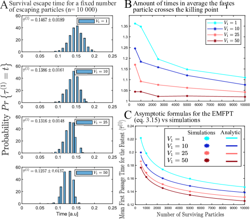
Figure 3: Influence of the killing rate on the mean escape time for the fastest particle. A. Stochastic simulations for the escape time distribution of the fastest particle $\bar{\tau}^{1}$ for particles distributed with respect to $p_{0}(x)=\delta(x-y)$ with $y=2$ and a killing point in $x_{1}=1$ for $n=10000$ with $1000$ runs. B. Decrease in the number of time the fastest particle crosses the killing point $x_{1}=1$ with the increasing of the killing weight for 1000 runs. C. EMFPT vs $n$ obtained from stochastic simulations (colored disks) and the asymptotic formulas (continuous lines) with $y=2$, $x_{1}=1$ and 1000 runs.

We decided to further explore the consequence of fixing the initial number of particles $N_{0}=$ [500 1000 2500 5000 10000], which does not necessarily correspond to the number of survival particles that will escape. In practice, much less particles will escape, thus reducing the total number used in the extreme statistics. To illustrate this difference, we plotted the mean escape time versus the killing term (Fig. 4A), and the EMFPT versus the killing probability (Fig. 4B). The curves differs from the result shown in Fig. 3, due to the decreasing in the number of survival particles. Such difference can be accounted for by adding a correction term $\alpha$ in the asymptotic formula for the EMFPT, as shown in Fig. 4B. When the killing weight $V_{1}$ increases, the number of escaping particles $n$ decreases, as shown in Fig. 4C. In that regime, the fastest particles also avoid crossing the killing point multiple times (Fig. 4D).

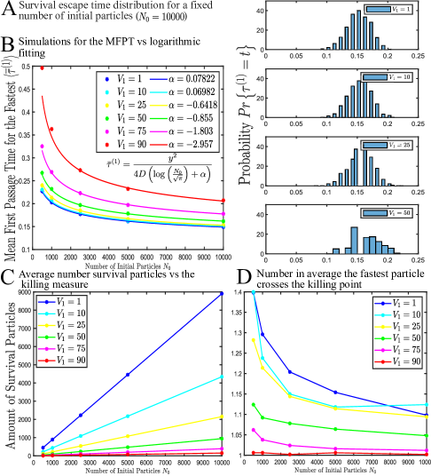
Figure 4: Influence of the killing rate on the escape time for a large number $N_{0}\gg 1$ of initial particles. A. Stochastic simulations for the escape time $\bar{\tau}^{1}$ distribution of the fastest particles, when the initial distribution is $p_{0}(x)=\delta(x-y)$ with $y=2$ and a killing measure at point $x_{1}=1$ for $N_{0}=10000$ with $1000$ runs. B. EMFPT vs $N_{0}$ obtained from stochastic simulations (colored disks) and the asymptotic formulas (continuous lines) with $y=2$, $x_{1}=1$ and 1000 runs. C. Influence of the killing weight $V_{1}$ in the number of survival particles. D. Decay of the number of time the fastest particle crosses the killing point $x_{1}=1$ when the killing weight increases (1000 runs).

4.2 Time scale of fast calcium signaling at synapse

Calcium dynamics at synapses is a fundamental step to transform neuronal spike coding, propagated across neurons into long-term molecular changes at a subcellular level, called synaptic plasticity, at the bases of learning and memory [25]. Interestingly, following a transient in the spine head (Fig. 5), fast calcium increase in dendrite is much faster than predicted by the classical transport resulting from the theory of diffusion [2]. This observation was interpreted as a consequence of the arrival of the fastest calcium ions that trigger calcium by a mechanism called calcium-induced-calcium-release through a class of receptor called Ryanodine receptor (RyR) located at the base of spine (Fig. 5). While the mean time of CICR was previously computed as the arrival of first two calcium ions to a RyR, this computed neglected the influence of calcium buffers that can capture calcium ion on their way for a long time, thus preventing a fast CICR. The main calcium buffers in the cytoplasm includes Trophin C, Calmodulin, Calcineurin and Myosin. If the concentration of buffer is high, the calcium trajectory that will arrive to a target will be significantly reduced. Calcium buffers could thus prevent the fast activation of CICR or even a second messenger pathway such as IP3 receptors, located at the base of a spine [43, 10, 42, 15].

4.2.1 Effect of calcium buffers modeled as a killing point source on Calcium-Induce-Calcium-Release

We propose now to model calcium dynamics in spine head as a diffusion in narrow cylinder, approximated as a segment. Indeed, due to the small size of the narrow cylinder and head of the dendritic spine, we could approximate the motion of calcium particles inside the narrow cylinder by a one dimensional Brownian motion in an interval. The fast binding to a buffer molecule will be account for by killing term in the diffusion equation, and since unbinding is often much longer that the binding time (hundreds vs few milliseconds), we can neglect here the unbinding time. The cases of uniform killing measures occurring on a interval is discussed in appendix Section 6. Some formula could be easily extended to the case of a partially absorbing target [12]. The effect of calcium removal by SERCA pumps can also be represented by a single or many killing points inside the interval $[0,L]$. The process of CICR induced by the binding of calcium ion to RyR is modeled as an absorbing boundary, where escape occurs.
We start the model, after there are a total of $n$ $Ca^{2+}$ ions that have entered the dendritic spine through the receptors (dark red point) located in the spine head (Fig. 5). The time of CICR is computed after the arrival of two fastest $Ca^{2+}$ ions at the RyR (blue dots) at the bottom of the spine (absorbing boundary condition). After the RyR is activated, an avalanche through a CIRC from SA is generated. This leads to an amplification of the calcium signal.

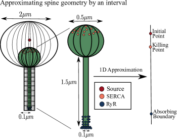
Figure 5: Schematic representation of a dendritic spine doted with a spine apparatus and its simplification in a 1D domain. The spine with a spine apparatus is simplified as a 1D interval with killing point $x_{1}=2\mu m$, initial point at $y=2.5\mu m$, absorbing point $x=0\mu m$.

The CICR process can be computed from the escape time distribution of the second fastest particle arriving to the absorbing end point of the interval, that model the spine neck. The pdf $Pr\left\{\bar{\tau}^{1}=s\right\}$ for the time the first ion arriving to the boundary allows to compute the pdf for second one to arrive by conditioning on the arrival of the first one at time s, while there are still $n-1$ ions in the interval. Thus we obtain the relation:

$$Pr\left\{\bar{\tau}^{2}=t\right\} = \int_{0}^{t}Pr\left\{\bar{\tau}^{2}=t|\bar{\tau}^{1}=s\right\}S^{n-1}(s)Pr\left\{\bar{\tau}^{1}=s\right\}ds$$

$$\sim \int_{0}^{t}Pr\left\{\bar{\tau}^{2}=t|\bar{\tau}^{1}=s\right\}Pr\left\{\bar{\tau}^{1}=s\right\}ds,$$

where we consider that the remaining $n-1$ particles are still alive close to the initial position when the killing weight $V_{1}$ is not too large, thus we use the approximation [2]

$$S^{n-1}(t)=\left(\int_{0}^{a}Pr\left\{x_{2}(t)=x_{2}\right\}dx_{2}\right)^{n-1}\approx 1.$$

We approximate the motion inside the narrow cylinder by a one dimensional Brownian motion in an interval $[0,L]$, with $y<L$, where $y$ is the initial position of the source, as shown in Fig. 5A. In practice $y=L$. The buffer or SERCA pumps are represented by a single killing point.
Using the approximation summarized by equation (28), and that $Pr\left\{\bar{\tau}^{2}=t|\bar{\tau}^{1}={\color[rgb]{1,0,0}s}\right\}\approx Pr\left\{\bar{\tau}^{1}=t-s\right\}$, the extreme escape time for the two fastest particles [2] is computed directly, leading to

(34) $$\bar{\tau}_{EMFPT}^{2}(n)\sim 2\bar{\tau}_{EMFPT}(n)\sim\frac{2L^{2}}{4D\left[\log\displaystyle\left(\frac{n}{\sqrt{\pi}}\right)-\log\left(1-\left(V_{1}\frac{x_{1}}{V_{1}|x_{1}|+D}\right)^{n}\right)\right]}.$$

To conclude, relation 34 shows that the consequence of the killing buffer is to decrease the binding time and the probability $1-\exp(-\frac{nA}{V_{1}})$, where $A\approx\frac{D}{|x_{1}|}$. Interestingly, the formula shows a modulation depending on the position of the killing source. For several killing- delta-Dirac, the extreme mean first passage is given by formula (21). When buffer molecules are uniformly distributed, formula (46) should be used instead.

4.2.2 Probability and time to induce long-term change at a molecular level

The second example we shall discuss consists in the molecular induction of plastic changes at a molecular level following high calcium concentration level entering into the neuronal synapse. The first step of the signaling consists in calcium ions binding to calmodulin and then the complex calcium-calmodulin needs to bind to a kinase third partner CaMKII [25]. We propose to estimate the probability to activate a given number $N_{KII}$ of CaMKII kinases inside a spine and how long does it takes for such activation.
We first consider that calcium bind quickly to calmodulin at the time scale given by the first ions to arrival to the molecule sites, of the order of less than 1 millisecond [13]. The unbinding time is too long (hundreds compared to few milliseconds). The binding of CaM containing a calcium to the kinase can be achieved by the four components: $CaMCa_{1}$, $CaMCa_{2}$, $CaMCa_{3}$ and $CaMCa_{4}$. This can be summarized by the following chemical rate equations:

(35) $$CAM+Ca^{2+} \leftrightharpoons CAMCa$$

(36) $$CAMCa+Ca^{2+} \leftrightharpoons CAMCa_{2}$$

(37) $$CAMCa_{2}+Ca^{2+} \leftrightharpoons CAMCa_{3}$$

(38) $$CAMCa_{3}+Ca^{2+} \leftrightharpoons CAMCa_{4}.$$

We consider the approximation that the number of molecules in each category is given by $N_{i}=p_{i}n$, where $p_{i}=p^{i}$ with $i=1,...,4$, where $p<1$. Thus the number of bound CaM to calcium decays exponentially with the initial number of calcium ions. The complex $CaMCa_{i}$ can dissociate with a rate $\kappa$ which is much shorter than the binding rate.
We apply now the result developed in the previous section to $CaMCa^{2+}_{i}$ $i=1,...,4,$ that can diffuse and thus escape the spine at the absorbing boundary. In that case, using relation (25), the probability that there are $N_{CaMKII}$ molecules of CaMKII bound by the population $CaMCa_{i}$ is given by the killing probability

(39) $$P_{i}=\left(\frac{x_{1}V_{1}}{V_{1}x_{1}+D}\right)^{N_{i}}.$$

Here we considered that the $CaMCa_{i}$ are located at position $x_{1}$ and $V_{1}$ represent the binding rate. When there are more CaMKII than CaM bound to calcium, then $V_{1}\approx k_{1}N_{CaMKII}$, where $k_{1}$ is the forward binding rate. In general, the mean number of bound CaMKII can be computed using a binomial law associated to $P_{i}$. Thus

(40) $$\langle CaMKII-CaMCa_{i}\rangle=P_{i}N_{CaMKII}$$

and the variance is $P_{i}(1-P_{i})N_{CaMKII}$. Finally, the total number of bound CaMKII is obtained by summing over $i=1,...,4$ as follows

(41) $$\langle CaMKII_{\hbox{bound}}\rangle=\sum_{i}\langle CaMKII-CaMCa_{i}\rangle=\sum_{i}N_{CaMKII}\left(\frac{V_{1}x_{1}}{V_{1}x_{1}+D}\right)^{np^{i}}.$$

The time of activation of the $CaMKII$ molecules by the population of $CaMCa_{2}$, which is the one that can lead to phosphorylation [25], keeping the kinase $CaMKII$ active, is given in our model by the time for the first killing to occur, as it represents the binding of $CaMCa_{2}$ to $CaMKII$. This time can be computed from formula (32) leading to

(42) $$\bar{\tau}^{k}_{EMFPT}(n)\sim\frac{\left(1-\left(\frac{\frac{D}{x_{1}V_{1}}}{1+\frac{D}{x_{1}V_{1}}}\right)^{p^{2}n}\right)(y-x_{1})^{2}}{4D\left(\frac{1}{1+\frac{D}{x_{1}V_{1}}}\right)^{p^{2}n}\left[\log\displaystyle\left(\frac{p^{2}nV_{1}(y-x_{1})}{4D\sqrt{\pi}\left(1-\left(\frac{\frac{D}{x_{1}V_{1}}}{1+\frac{D}{x_{1}V_{1}}}\right)^{p^{2}n}\right)}\right)\right]},$$

where $D=100\mu m^{2}/s$, $n=50000$, $y=1\mu m$, $x_{1}=0.1\mu m$, $p=0.2$ [13], $V_{1}$ is not known but it could be found from experiments. For instance if $k_{1}=50\mu m/s$, we can find the mean time for activate the $CaMKII$ from replacing all this values in the formula, and thus we obtain $\bar{\tau}^{k}_{EMFPT}=0.0079s$, meaning that the activation of this molecules is in the order of a few milliseconds.

5 Conclusions and perspective

We reported here various escape asymptotic laws for the fastest particles to reach the boundary of an interval when there are multiple delta-Dirac killing sources. We obtain asymptotic formula for the large number of particle limit. The formulas revealed the mixed role of dynamics and killing that influences the fastest particle to escape.
We used this framework to estimate how buffer can influence calcium dynamics at synapses in the process of calcium induce calcium release and the time of $CaMKII$ activation. In general, the present approach can be used to derive the time scale of biochemical processes, where signaling occurs through the fastest particles. This framework can also account for the time to activate an ensemble of chemical processes [28] or the time for a chemical message to be delivered when it is carried by few particles among many [44, 4, 8]. Finding a target is key to activate sub-cellular process [40]. However, during this event, the diffusing messenger can bind to molecules that can trap or destroy them, thus affecting the path of the fastest particles to their final target. These binding molecules can diminish the arrival probability, but interestingly, they reduce the time of arrival, as shown by formulas 28, 6.1, 44, 46 and 47: indeed, the fastest particles should avoid staying in the domain where they can terminated, easier with point wise or uniform killing distribution. These formula further reveal that the distribution of killing sources influences on the fastest escape time.
There are other examples where the present theory could be relevant: in the cell nucleus [30], transcription factors (TFs) are switching between different states before escaping to a small target site: the $TFs$ are moving as a Brownian particles and can bind to various ligands to change state (acethylation or sumolysation) [1]. The TFs can be degraded, preventing the fastest to reach the target, while gene activation can only occur in one of the appropriate state. This example shows that the number of TFs can accelerate the production of mARN, but the escape time could be limited by killing processes. Finally, it would be interesting to extend the present study in higher dimensions where the fastest can avoid entering the killing region.

6 Appendix

We presented in this appendix the computations for the mean first escape time when the killing measure is uniform and located in an interval that may or may not contain the initial point.

6.1 Escape for the fastest with a uniform killing in half-a-line

We now consider the escape time for the fastest particle when the killing measure $k\left(x,t\right)=V_{0}$ is constant over the half-a-line $x\geq 0$. The diffusion coefficient is $D$ and the survival FPE for each individual particle is

$$\frac{\partial p(x,t\,|\,y)}{\partial t} = D\frac{\partial^{2}p(x,t\,|\,y)}{\partial x^{2}}-V_{0}p(x,t\,|\,y),\quad\mbox{for $x\in\mathbb{R}_{+},\ t>0$}$$

$$p(x,0\,|\,y) = \delta(y-x)$$

$$p(0,t\,|\,y) = 0.$$

The solution of this equation is given by

$$p(x,t\,|\,y)=\exp\left\{-V_{0}t\right\}\frac{1}{2\sqrt{\pi Dt}}\left(\exp\left\{-\frac{(x-y)^{2}}{4Dt}\right\}-\exp\left\{-\frac{(x+y)^{2}}{4Dt}\right\}\right)$$

and the flux is

$$J(t\,|\,y)=D\frac{\partial p}{\partial x}(x=0,t\,|\,y)=\exp\left\{-V_{0}t\right\}\frac{y}{t\sqrt{4\pi Dt}}\left(\exp\left\{-\frac{y^{2}}{4Dt}\right\}\right).$$

Thus using the inverse Laplace transform

$$\int_{0}^{\infty}\frac{1}{\sqrt{\pi}t^{3/2}}e^{-at-b/t}dt=\frac{1}{2\sqrt{b}}\exp\left\{-2\sqrt{ab}\right\},$$

we find the expression for the probability to escapes alive for one particle

$$\int_{0}^{\infty}J(t\,|\,y)dt=\exp\left\{-y\sqrt{\frac{V_{0}}{D}}\right\}.$$

Thus, the probability that the first one escape alive in an ensemble of $n$ is

$$P_{\infty}=1-\left(1-\int_{0}^{\infty}J(t\,|\,y)dt\right)^{n}=1-\left(1-\exp\left\{-y\sqrt{\frac{V_{0}}{D}}\right\}\right)^{n}.$$

Similarly, we obtain the expression for the total flux for a single particle

$$\int_{0}^{t}J(s\,|\,y)ds=\int_{0}^{t}\frac{y\exp\left\{-V_{0}s\right\}\exp\left\{-\frac{y^{2}}{4Ds}\right\}}{\sqrt{4D\pi s}s}ds$$

$$= \frac{1}{2}\left(\exp\left\{-y\sqrt{\frac{V_{0}}{D}}\right\}\mathrm{erfc}\left(\frac{y}{\sqrt{4Dt}}-\sqrt{V_{0}t}\right)+\exp\left\{y\sqrt{\frac{V_{0}}{D}}\right\}\mathrm{erfc}\left(\frac{y}{\sqrt{4Dt}}+\sqrt{V_{0}t}\right)\right).$$

For $t$ small, using the expansion for the complementary error function for large arguments we compute the numerator of the EMFPT (relation 3.1) as

$$s(t) \sim \left(1-\frac{e^{-\frac{y^{2}}{4Dt}}\sqrt{4Dt}}{y\sqrt{\pi}}\frac{\left(e^{-y\sqrt{\frac{V_{0}}{D}}}+e^{y\sqrt{\frac{V_{0}}{D}}}\right)}{2}\right)^{n}-\left(1-e^{-y\sqrt{\frac{V_{0}}{D}}}\right)^{n}$$

$$\sim 1-\left(1-e^{-y\sqrt{\frac{V_{0}}{D}}}\right)^{n}+\sum_{k=1}^{n}\binom{n}{k}\left(\frac{e^{-\frac{y^{2}}{4Dt}}\sqrt{4Dt}}{y\sqrt{\pi}}\frac{\left(e^{-y\sqrt{\frac{V_{0}}{D}}}+e^{y\sqrt{\frac{V_{0}}{D}}}\right)}{2}\right)^{k}.$$

This, leads to the following integral dominated for $t$ small when $n$ large,

$$\bar{\tau}_{EMFPT}(n) \sim \int\limits_{0}^{\delta}\left[1-n\frac{\sqrt{4Dt}\exp\left\{-\frac{y^{2}}{4Dt}\right\}\left(e^{-y\sqrt{\frac{V_{0}}{D}}}+e^{y\sqrt{\frac{V_{0}}{D}}}\right)}{2y\sqrt{\pi}\left(1-\left(1-e^{-y\sqrt{\frac{V_{0}}{D}}}\right)^{n}\right)}\right]\,dt$$

$$\sim \int\limits_{0}^{\infty}\exp\left\{-n\frac{\sqrt{4Dt}\exp\left\{-\frac{y^{2}}{4Dt}\right\}\left(e^{-y\sqrt{\frac{V_{0}}{D}}}+e^{y\sqrt{\frac{V_{0}}{D}}}\right)}{2y\sqrt{\pi}\left(1-\left(1-e^{-y\sqrt{\frac{V_{0}}{D}}}\right)^{n}\right)}\right\}\,dt,$$

and proceeding as in [2], we get

(44) $$\bar{\tau}_{EMFPT}(n) \sim \frac{y^{2}}{4D\log\displaystyle\left(\frac{n\left(e^{-y\sqrt{\frac{V_{0}}{D}}}+e^{y\sqrt{\frac{V_{0}}{D}}}\right)}{2\sqrt{\pi}\left(1-\left(1-e^{-y\sqrt{\frac{V_{0}}{D}}}\right)^{n}\right)}\right)}.$$

Note that, when $V_{0}=0$, we recover the asymptotic formula for the case without killing and a Dirac-delta function as initial condition.

6.2 Killing in a finite interval in half a line with initial point outside the interval

We consider the diffusion of a particle that starts at a point $y$ outside the interval $[0,L]$. The pdf of that particle’s trajectory satisfies the equation

(45) $$\frac{\partial p(x,t\,|\,y)}{\partial t} = D\frac{\partial^{2}p(x,t\,|\,y)}{\partial x^{2}}-V\chi_{[0,L]}(x)p(x,t\,|\,y)\quad\hbox{ on }\mathbf{R}_{+}$$

$$p(x,0\,|\,y) = \delta(x-y)$$

$$p(0,t\,|\,y) = 0.$$

To compute the explicit solution, $p(x,t\,|\,\mbox{\boldmath$y$})$, we Laplace transform the equation with respect to $t$ and we obtain the equation

$$\frac{\partial^{2}u}{\partial x^{2}}(x,q)-\left(\frac{q+V}{D}\right)u(x,q)=0\,\,\,\,\,\text{for $x\in[0,L]$}$$

$$\frac{\partial^{2}u}{\partial x^{2}}(x,q)-\left(\frac{q}{D}\right)u(x,q)=-\frac{1}{D}\delta(x-y)\,\,\,\,\,\text{for $x\in(L,+\infty)$},$$

where $u(x,q)=\mathcal{L}\left(p(x,t\,|\,\mbox{\boldmath$y$})\right)$, and the bounded solutions in $\mathbf{R}_{+}$ are in the form

$$u(x,q)=A\exp\left\{-\sqrt{\frac{q+V}{D}}x\right\}-A\exp\left\{\sqrt{\frac{q+V}{D}}x\right\}\,\,\,\,\,\text{for $x\in[0,L]$}$$

$$u(x,q)=\frac{1}{\sqrt{4Dq}}\exp\left\{-\sqrt{\frac{q}{D}}|x-y|\right\}+B\exp\left\{-\sqrt{\frac{q}{D}}|x+y|\right\}\,\,\,\,\,\text{for $x\in(L,+\infty)$}.$$

We are looking for the solutions that are continuous at $x=L$ and its first derivative is also continuous at $x=L$, then solving the corresponding system we get

$$A = -\frac{e^{\sqrt{\frac{q}{D}}(L-y)}}{D\left(\left(\sqrt{\frac{q+V}{D}}-\sqrt{\frac{q}{D}}\right)e^{-\sqrt{\frac{q+V}{D}}L}+\left(\sqrt{\frac{q+V}{D}}+\sqrt{\frac{q}{D}}\right)e^{\sqrt{\frac{q+V}{D}}L}\right)},$$

$$B = \displaystyle\frac{\left(\sqrt{\frac{q+V}{D}}-\sqrt{\frac{q}{D}}\right)e^{-\left(\sqrt{\frac{q+V}{D}}-2\sqrt{\frac{q}{D}}\right)L}-\left(\sqrt{\frac{q+V}{D}}-\sqrt{\frac{q}{D}}\right)e^{\left(\sqrt{\frac{q+V}{D}}+2\sqrt{\frac{q}{D}}\right)L}}{\sqrt{4Dq}\left(\left(\sqrt{\frac{q+V}{D}}-\sqrt{\frac{q}{D}}\right)e^{-\sqrt{\frac{q+V}{D}}L}+\left(\sqrt{\frac{q+V}{D}}+\sqrt{\frac{q}{D}}\right)e^{\sqrt{\frac{q+V}{D}}L}\right)}.$$

Using relation (5), we have

$$\int_{0}^{\infty}J(t)dt=D\int_{0}^{t}\frac{\partial p}{\partial x}(x=0,t|\,y)\,dt=D\frac{\partial u}{\partial x}(0,0)=\frac{1}{\cosh\left(\sqrt{\frac{V}{D}}L\right)}.$$

For $t$ small, we have

$$\int_{0}^{t}J(s)ds = D\int_{0}^{t}\frac{\partial p}{\partial x}(x=0,s|\,y)\,ds\sim\int_{0}^{t}\left[\mathcal{L}^{-1}_{s}\left(e^{-y\sqrt{\frac{q}{D}}}\right)-VL\mathcal{L}^{-1}_{s}\left(\frac{e^{-y\sqrt{\frac{q}{D}}}}{\sqrt{4Dq}}\right)\right]ds$$

$$\sim \mathrm{erfc}\left(\frac{y}{\sqrt{4Dt}}\right).$$

Then, we have

$$P_{\infty}=1-\left(1-\int_{0}^{\infty}J(t\,|\,\mbox{\boldmath$y$})dt\right)^{n}=1-\left(1-\frac{1}{\cosh\left(\sqrt{\frac{V}{D}}L\right)}\right)^{n},$$

and

$$s(t) \sim \left(1-\frac{e^{-\frac{y^{2}}{4Ds}}\sqrt{4Dt}}{y\sqrt{\pi}}\right)^{n}-\left(1\frac{1}{\cosh\left(\sqrt{\frac{V}{D}}L\right)}\right)^{n}$$

$$\sim 1-\left(1-\frac{1}{\cosh\left(\sqrt{\frac{V}{D}}L\right)}\right)^{n}+\sum_{k=1}^{n}\binom{n}{k}\left(\frac{e^{-\frac{y^{2}}{4Ds}}\sqrt{4Dt}}{y\sqrt{\pi}}\right)^{k}.$$

This, leads to the following integral dominated for $t$ small when $n$ large

$$\bar{\tau}_{EMFPT}(n) \sim \int\limits_{0}^{\delta}\left[1-n\frac{\sqrt{4Dt}\exp\left\{-\frac{y^{2}}{4Dt}\right\}}{y\sqrt{\pi}\left(1-\left(1-\frac{1}{\cosh\left(\sqrt{\frac{V}{D}}L\right)}\right)^{n}\right)}\right]\,dt$$

$$\sim \int\limits_{0}^{\infty}\exp\left\{-n\frac{\sqrt{4Dt}\exp\left\{-\frac{y^{2}}{4Dt}\right\}}{y\sqrt{\pi}\left(1-\left(1-\frac{1}{\cosh\left(\sqrt{\frac{V}{D}}L\right)}\right)^{n}\right)}\right\}\,dt,$$

and proceeding as in [2], we get

(46) $$\displaystyle\bar{\tau}_{EMFPT}(n) \sim \frac{y^{2}}{4D\log\left(\frac{n}{\sqrt{\pi}\left(1-\left(1-\frac{1}{\cosh\left(\sqrt{\frac{V}{D}}L\right)}\right)^{n}\right)}\right)}.$$

Note that, when $V=0$, we recover the asymptotic formula for the case without a killing term and a Dirac-delta function as initial condition.

6.3 Killing in a finite interval in half a line with initial point inside the interval

In this case, we consider the diffusion of a particle that starts at a point $y$ inside the interval $[0,L]$, then the pdf of the particle’s trajectory satisfies the equation (45) but when we apply the Laplace transform to this equation, we get

$$\frac{\partial^{2}u}{\partial x^{2}}(x,q)-\left(\frac{q+V}{D}\right)u(x)=-\frac{1}{D}\delta(x-y)\hskip 31.2982pt\text{for $x\in[0,L]$}$$

$$\frac{\partial^{2}u}{\partial x^{2}}(x,q)-\left(\frac{q}{D}\right)u(x)=0\hskip 99.58464pt\text{for $x\in(L,+\infty)$},$$

where $u(x,q)=\mathcal{L}\left(p(x,t\,|\,\mbox{\boldmath$y$})\right)$. Here, the bounded solutions in $\mathbf{R}_{+}$ are in the form

$$u(x,q)=A\left(\exp\left\{-\sqrt{\frac{q+V}{D}}|x-y|\right\}-\exp\left\{-\sqrt{\frac{q+V}{D}}|x+y|\right\}\right)$$

$$+ \left(A-\frac{1}{\sqrt{4D(q+V)}}\right)\left(\exp\left\{\sqrt{\frac{q+V}{D}}|x-y|\right\}-\exp\left\{\sqrt{\frac{q+V}{D}}|x+y|\right\}\right)\,\,\,\text{for $x\in[0,L]$}$$

$$u(x,q)=B\exp\left\{-\sqrt{\frac{q}{D}}x\right\}\,\,\,\text{for $x\in(L,+\infty)$}.$$

Because we are looking for the continuous solutions at $x=L$ with first derivative continuous at $x=L$, we can solve the corresponding system and we get

$$A = \scriptstyle\frac{-\left(\sqrt{\frac{q+V}{D}}+\sqrt{\frac{q}{D}}\right)\left(e^{\sqrt{\frac{q+V}{D}}(L-y)}-e^{\sqrt{\frac{q+V}{D}}(L+y)}\right)\frac{1}{\sqrt{4D(q+V)}}}{\left(\left(\sqrt{\frac{q+V}{D}}-\sqrt{\frac{q}{D}}\right)\left(e^{-\sqrt{\frac{q+V}{D}}(L-y)}-e^{-\sqrt{\frac{q+V}{D}}(L+y)}\right)-\left(\sqrt{\frac{q+V}{D}}+\sqrt{\frac{q}{D}}\right)\left(e^{\sqrt{\frac{q+V}{D}}(L-y)}-e^{\sqrt{\frac{q+V}{D}}(L+y)}\right)\right)},$$

$$B = \scriptstyle\frac{e^{-\sqrt{\frac{q}{D}}L}}{D\left(\left(\sqrt{\frac{q+V}{D}}-\sqrt{\frac{q}{D}}\right)\left(e^{-\sqrt{\frac{q+V}{D}}(L-y)}-e^{-\sqrt{\frac{q+V}{D}}(L+y)}\right)-\left(\sqrt{\frac{q+V}{D}}+\sqrt{\frac{q}{D}}\right)\left(e^{\sqrt{\frac{q+V}{D}}(L-y)}-e^{\sqrt{\frac{q+V}{D}}(L+y)}\right)\right)}.$$

Using relation (5), we have

$$\int_{0}^{\infty}J(t)dt=D\int_{0}^{t}\frac{\partial p}{\partial x}(x=0,t|\,y)\,dt=D\frac{\partial u}{\partial x}(0,0)=\exp\left\{-y\sqrt{\frac{V}{D}}\right\}.$$

For $t$ small, we get

$$\int_{0}^{t}J(s)ds = D\int_{0}^{t}\frac{\partial p}{\partial x}(x=0,s|\,y)\,ds=\int_{0}^{t}\mathcal{L}^{-1}_{s}\left(e^{-y\sqrt{\frac{q}{D}}}\right)ds=\mathrm{erfc}\left(\frac{y}{\sqrt{4Dt}}\right).$$

Then, as in the case for the uniform killing, we get the asymptotic formula

(47) $$\displaystyle\bar{\tau}_{EMFPT}(n) \sim \frac{y^{2}}{4D\log\left(\displaystyle\frac{n\left(e^{-y\sqrt{\frac{V}{D}}}+e^{y\sqrt{\frac{V}{D}}}\right)}{2\sqrt{\pi}\left(1-\left(1-e^{-y\sqrt{\frac{V}{D}}}\right)^{n}\right)}\right)}.$$

References

• [1] Bruce Alberts, Dennis Bray, Karen Hopkin, Alexander D Johnson, Julian Lewis, Martin Raff, Keith Roberts, and Peter Walter. Essential cell biology. Garland Science, 2013.
• [2] K Basnayake, Zeev Schuss, and David Holcman. Asymptotic formulas for extreme statistics of escape times in 1, 2 and 3-dimensions. Journal of Nonlinear Science, 29(2):461–499, 2019.
• [3] Kanishka Basnayake and David Holcman. Fastest among equals: a novel paradigm in biology. reply to comments: Redundancy principle and the role of extreme statistics in molecular and cellular biology. Physics of life reviews, 28:96–99, 2019.
• [4] Kanishka Basnayake and David Holcman. Fastest among equals: a novel paradigm in biology. reply to comments: Redundancy principle and the role of extreme statistics in molecular and cellular biology. Physics of life reviews, 28:96–99, 2019.
• [5] Kanishka Basnayake, David Mazaud, Alexis Bemelmans, Nathalie Rouach, Eduard Korkotian, and David Holcman. Fast calcium transients in dendritic spines driven by extreme statistics. PLoS biology, 17(6), 2019.
• [6] Simeon M Berman and Frydman Halina. Distributions associated with markov processes with killing. Stochastic Models, 12(3):367–388, 1996.
• [7] Subrahmanyan Chandrasekhar. Stochastic problems in physics and astronomy. Reviews of modern physics, 15(1):1, 1943.
• [8] Daniel Coombs. First among equals: Comment on “redundancy principle and the role of extreme statistics in molecular and cellular biology” by Z. Schuss, K. Basnayake and D. Holcman. Physics of life reviews, 2019.
• [9] Geneviève Dupont, Martin Falcke, Vivien Kirk, and James Sneyd. Models of calcium signalling, 2016.
• [10] Geneviève Dupont and James Sneyd. Recent developments in models of calcium signalling. Current opinion in systems biology, 3:15–22, 2017.
• [11] Crispin W Gardiner et al. Handbook of stochastic methods, volume 3. springer Berlin, 1985.
• [12] Denis Grebenkov, Ralf Metzler, and Gleb Oshanin. From single-particle stochastic kinetics to macroscopic reaction rates: fastest first-passage time of $n$ random walkers. New Journal of Physics, 2020.
• [13] D Holcman, Z Schuss, and E Korkotian. Calcium dynamics in dendritic spines and spine motility. Biophysical journal, 87(1):81–91, 2004.
• [14] David Holcman, Avi Marchewka, and Zeev Schuss. The survival probability of diffusion with killing. arXiv preprint math-ph/0502035, 2005.
• [15] David Holcman and Zeev Schuss. Modeling calcium dynamics in dendritic spines. Siam Journal on Applied Mathematics, 65(3):1006–1026, 2005.
• [16] David Holcman and Zeev Schuss. Stochastic narrow escape in molecular and cellular biology. Analysis and Applications. Springer, New York, 2015.
• [17] David Holcman and Zeev Schuss. Stochastic Narrow Escape in Molecular and Cellular Biology: Analysis and Applications. Springer, 2015.
• [18] Hye-Won Kang and Radek Erban. Multiscale stochastic reaction–diffusion algorithms combining markov chain models with stochastic partial differential equations. Bulletin of mathematical biology, 81(8):3185–3213, 2019.
• [19] Samuel Karlin and Simon Tavaré. A diffusion process with killing: the time to formation of recurrent deleterious mutant genes. Stochastic Processes and their Applications, 13(3):249–261, 1982.
• [20] Samuel Karlin and Simon Tavaré. A class of diffusion processes with killing arising in population genetics. SIAM Journal on Applied Mathematics, 43(1):31–41, 1983.
• [21] T Lagache, E Dauty, and D Holcman. Physical principles and models describing intracellular virus particle dynamics. Current opinion in microbiology, 12(4):439–445, 2009.
• [22] Thibault Lagache, Emmanuel Dauty, and David Holcman. Quantitative analysis of virus and plasmid trafficking in cells. Physical Review E, 79(1):011921, 2009.
• [23] Sean D Lawley. Distribution of extreme first passage times of diffusion. Journal of Mathematical Biology, pages 1–25, 2020.
• [24] Sean D. Lawley. Extreme first-passage times for random walks on networks. Phys. Rev. E, 102(6):062118, 14, 2020.
• [25] Joel Lee, Xiumin Chen, and Roger A Nicoll. Synaptic memory survives molecular turnover. Proceedings of the National Academy of Sciences, 119(42):e2211572119, 2022.
• [26] Katja Lindenberg, Ralf Metzler, and Gleb Oshanin. Chemical Kinetics: Beyond the Textbook. World Scientific Publishing Europe Ltd, 2019.
• [27] Samantha Linn and Sean D Lawley. Extreme hitting probabilities for diffusion. Journal of Physics A: Mathematical and Theoretical, 55(34):345002, 2022.
• [28] Ting Lu, Tongye Shen, Chenghang Zong, Jeff Hasty, and Peter G Wolynes. Statistics of cellular signal transduction as a race to the nucleus by multiple random walkers in compartment/phosphorylation space. Proceedings of the National Academy of Sciences, 103(45):16752–16757, 2006.
• [29] Jingwei Ma, Myan Do, Mark A Le Gros, Charles S Peskin, Carolyn A Larabell, Yoichiro Mori, and Samuel A Isaacson. Strong intracellular signal inactivation produces sharper and more robust signaling from cell membrane to nucleus. PLoS computational biology, 16(11):e1008356, 2020.
• [30] G Malherbe and D Holcman. The search for a dna target in the nucleus. Physics Letters A, 374(3):466–471, 2010.
• [31] LM Martyushev. Minimal time, weibull distribution and maximum entropy production principle: Comment on” redundancy principle and the role of extreme statistics in molecular and cellular biology” by z. schuss et al. Physics of life reviews, 2019.
• [32] Alain Mazzolo and Cécile Monthus. Conditioning diffusion processes with killing rates. arXiv preprint arXiv:2204.05607, 2022.
• [33] Baruch Meerson and S Redner. Mortality, redundancy, and diversity in stochastic search. Physical review letters, 114(19):198101, 2015.
• [34] Ralf Metzler, Sidney Redner, and Gleb Oshanin. First-passage phenomena and their applications, volume 35. World Scientific, 2014.
• [35] S Redner and B Meerson. Redundancy, extreme statistics and geometrical optics of brownian motion: Comment on” redundancy principle and the role of extreme statistics in molecular and cellular biology” by z. schuss et al. Physics of life reviews, 2019.
• [36] Karine Reynaud, Zeev Schuss, Nathalie Rouach, and David Holcman. Why so many sperm cells? Communicative & integrative biology, 8(3):e1017156, 2015.
• [37] Hannes Risken. Fokker-planck equation. In The Fokker-Planck Equation, pages 63–95. Springer, 1996.
• [38] Dmitri A Rusakov and Leonid P Savtchenko. Extreme statistics may govern avalanche-type biological reactions: Comment on” redundancy principle and the role of extreme statistics in molecular and cellular biology” by z. schuss, k. basnayakey, d. holcman. Physics of life reviews, 2019.
• [39] Grégory Schehr and Satya N Majumdar. Exact record and order statistics of random walks via first-passage ideas. In First-Passage Phenomena and Their Applications, pages 226–251. World Scientific, 2014.
• [40] Z Schuss, K Basnayake, and D Holcman. Redundancy principle and the role of extreme statistics in molecular and cellular biology. Physics of life reviews, 2019.
• [41] Zeev Schuss. Stochastic differential equations. In Theory and Applications of Stochastic Processes, pages 92–132. Springer, 2010.
• [42] Godfrey L Smith and David A Eisner. Calcium buffering in the heart in health and disease. Circulation, 139(20):2358–2371, 2019.
• [43] James Sneyd, Joel Keizer, and Michael J Sanderson. Mechanisms of calcium oscillations and waves: a quantitative analysis. The FASEB Journal, 9(14):1463–1472, 1995.
• [44] Igor M. Sokolov. Extreme fluctuation dominance in biology: On the usefulness of wastefulness: Comment on “redundancy principle and the role of extreme statistics in molecular and cellular biology” by Z. Schuss, K. Basnayake and D. Holcman. Physics of life reviews, 2019.
• [45] M.V. Tamm. Importance of extreme value statistics in biophysical contexts: Comment on “redundancy principle and the role of extreme statistics in molecular and cellular biology”. Physics of life reviews, 2019.
• [46] Suney Toste and David Holcman. Asymptotics for the fastest among n stochastics particles: role of an extended initial distribution and an additional drift component. Journal of Physics A: Mathematical and Theoretical, 2021.
• [47] George H Weiss. A perturbation analysis of the wilemski–fixman approximation for diffusion-controlled reactions. The Journal of chemical physics, 80(6):2880–2887, 1984.
• [48] George H Weiss, Kurt E Shuler, and Katja Lindenberg. Order statistics for first passage times in diffusion processes. Journal of Statistical Physics, 31(2):255–278, 1983.
• [49] J Yang, I Kupka, Z Schuss, and D Holcman. Search for a small egg by spermatozoa in restricted geometries. Journal of mathematical biology, 73(2):423–446, 2016.
• [50] Rafael Yuste. Dendritic spines. MIT press, 2010.
• [51] S. B. Yuste and K. Lindenberg. Order statistics for first passage times in one-dimensional diffusion processes. J. Stat. Phys., 85:501–512, 1996.