Darboux Wronskian solutions of Ito typed coupled KdV equation with exact solitonic solutions and conserved densities

Abstract

In this article, we derive the Darboux solutions of Ito type coupled KdV equation in Darboux framework which is associated with Hirota Satsuma systems. Then we generalise $N$-fold Darboux transformations in terms of Wronskians. We also derive the exact multi-solitonic solutions for the coupled field variables of that system in the background of zero seed solutions. The last section encloses the derivation of continuity equation with several conserved densities through its Riccati equation.

[a]organization=Department of Mathematics, , addressline= Colllege of Science, Shanghai University, city=Shanghai, country=200444, P.R.China

[b]organization=Centre for High Energy Physics, addressline=University of the Punjab, city=Lahore, postcode=54590, state=Punjab, country=Pakistan

1 Introduction

The nonlinear solitonic equations have got considerable attentions in theory of integrable systems because of their wide applications in various domains of physics and applied mathematics. One of the very interesting and earliest solitonic equations is KdV equation that plays a crucial role in the study of hydrodynamics to describe the geometrical properties of wave propagations in shallow water [1] and has also been acknowledged as integrable model in the analysis of electron plasma waves phenomenon associated with cylindrical plasma system [2]. The study of solitonic solutions of nonlinear evolution equations attained substantial importance in modern theory of integrable systems in exploring algebraic and geometrical profiles with their physical aspects, for example in context of Bose-Einstein condensate different types of solitons such as bright solitons [3, 4] dark solitons [4], vortex solitons [5] and gap solitons [6] have been found while studying matter wave solitons. In this article we construct the solitonic solutions of Ito type coupled KdV equation wave equation

$$\left\{\begin{array}[]{lr}u_{t}=u_{xxx}+6uu_{x}+q_{x}\\ v_{t}=2(uv)_{x}\end{array}\right.$$ (1)

which also called Integrable coupled nonlinear wave. The above coupled nonlinear wave (CNW) equation (1) with $q=v^{2}$ can be obtained as the parametric reduction of famous Ito system [7] has been applied as integrable model in various domains of physics and fluid mechanics. Recently, its integro-differential analogue [8] with mixed dark-bright solitonic solutions have been investigated. Moreover, that coupled nonlinear wave equation has earned much importance in theory of integrable systems as it involves the KdV structure and reduces to the ordinary KdV equation by setting the coupling variables $v$ as $v=0$. Here, we apply Darboux transformation to investigate its solitonic solutions. That Darboux approach [9, 10, 11] has been acknowledged as one of the efficient tools in theory of integrable systems to calculate the exact solutions of these systems with their algebraic and geometrical properties. In literature number of successful implementations of this transformation have been shown as an efficient integrable tool which enhance its significance from physical point of views. Among these number of remarkable applications of DT few of them are mentioned here as applied in the analysis of electrodynamical features [12] in case of quantum cavity problems and also to investigate the geometrical properties of graphene [13] with exact solitonic solutions. Moreover, that method has also been applied fruitfully to construct the quasideterminant solutions of the Painlevé II equation [14] with its related Toda system [15] for its non-commutative analogs and to derive the exact solutions of the generalized coupled dispersionless integrable system[16]. In section $2$, we construct one-fold, two-fold and three-fold Darboux solutions of equation (1) with the help of linear representation for its coupling field variable $u$ and $v$ and then we generalise its $N$-fold Darboux solutions in determinantal form as in terms of Wronskians.

Subsequently, we derive exact multi-solitonic solutions in the background of zero seed solutions for both coupling field variables $u$ and $q$ with graphical presentations of variety of solutions scattering elastically. This work also encloses the derivation of matrix zero curvature representation of CNW equation (1) possessing traceless matrices through its existed scalar Lax pair. That representation may be assumed to fit in the AKNS scheme [17] as it usually involves the parametric traceless matrices of order $N$ containing field variables. In last section we derive equation of continuity through the linear representation of CNW equation (1). We also calculate its several conserved densities with the help of its Riccati equation.

2 Linear representations and The Darboux solutions

This section encloses the Lax representation of Ito type coupled KdV equation which also called Integrable coupled nonlinear wave (CNW) equation (1) and the derivation of its equivalent zero-curvature from scalar Lax pair. Then by using the Darbaoux transformation [9, 10] on arbitrary function we construct the one-fold, two-fold and three-fold Darboux solutions to coupling field variables $u$ and $v$ in terms of seed solutions. Subsequently we generalize their $N$-fold Darboux solutions in determinantal form.

2.1 Lax Pair and Zero-curvature representation

The coupled nonlinear wave equation (1) possesses is integrable [18, 19] and arises as the compatibility of subsequent linear system

$$\psi_{xx}=\left(\lambda-u-\beta q\right)\psi.\\$$ (2)

$$\psi_{t}=\left(4\lambda+2u\right)\psi_{x}-u_{x}\psi.$$ (3)

where $q=v^{2}$ , $\beta=\frac{1}{4\lambda}$ and $\lambda$ is spectral parameter. It is easy to obtain CNW equation (1) by elimination of arbitrary function $\psi_{xx}$ from above linear system.

Proposition 2.1

By introducing a column vector in terms of arbitrary function as $F=(f_{0},f_{1})^{T}=(\psi,\psi_{x})^{T}$, we may construct the matrix zero-curvature representation of CNW equation (1).

Proof

Consider the following linear system for arbitrary function $F$

$$\left\{\begin{array}[]{lr}\partial_{x}F=AF\\ \partial_{t}F=BF\end{array}\right.,$$ (4)

where $A$ and $B$ are the matrices of order $2$ to be determined, the compatibility of linear system (4) yields zero-curvature form as below

$$\partial_{t}A-\partial_{x}B+[A,B]=0,$$ (5)

This can be shown that with the help of $F=(f_{0},f_{1})^{T}=(\psi,\psi_{x})^{T}$, the eigenvalue equation $L\psi=\lambda\psi$ will take the following form

$$\partial_{x}(f_{0},f_{1})^{T}=A(f_{0},f_{1})^{T},$$ (6)

where $A=\begin{bmatrix}0&1\\ \lambda-u-\beta q&0\end{bmatrix}$ and can also be written as $F_{x}=AF$. For the temporal part, let take the derivatiion of $\psi_{t}=\left(4\lambda+2u\right)\psi_{x}-u_{x}\psi$ with respect to $x$, then by using $\psi_{xx}=\left(\lambda-u-\beta q\right)\psi$ in resulting expression , we get

$$\psi_{tx}=u_{x}\psi_{x}+4\lambda^{2}\psi-2\lambda u\psi-v^{2}\psi-2u^{2}\psi-\frac{uv^{2}\psi}{2\lambda}-u_{xx}\psi,$$ (7)

Now combining equation (3) and above equation, we obtain $F_{t}=BF$, where

$$B=\begin{bmatrix}-u_{x}&4\lambda+2u\\ 4\lambda^{2}-2\lambda u-v^{2}-2u^{2}-\frac{uv^{2}}{2\lambda}-u_{xx}&u_{x}\end{bmatrix},$$ (8)

Remark

The above matrix zero-curvature representation is derived from its scalar analogue presented in [18] whose compatibility condition is equivalent to ito type system as CNW equation (1) and the method mentioned above is straight forward to calculate the matrix zero curvatue representation from existed scalar Lax pair.

2.2 Darboux solutions

Here we construct the explicit Darboux expressions for the field variables $u$ and $v$ which connect the old solutions of CNW equation (1) to its new solutions through the particular solutions of linear equations (2) and (3). In order to construct the Darboux solutions for the coupled field variables $u$ and $v$, let $u[1]$ and $q[1]$ are new solutions of CNW equation (1) and $\psi[1]$ is also a new solution of its associated linear system, then linear equation (2) with these new solution becomes

$$\psi_{xx}[1]=\left(\lambda-u[1]-\beta q[1]\right)\psi[1],$$ (9)

the transformation on arbitrary function is defined as

$$\psi[1]=\psi_{x}-\sigma_{1}\psi,$$ (10)

where $\sigma_{1}=\frac{\psi_{1x}}{\psi_{1}}$ and the $\psi_{1}$ is a particular solution can be calculated at $\lambda=\lambda_{1x}$ from linear system (2) and (3) with provided seed solutions. Now substitute the value of $\psi[1]$ from equation (10) into transformed expression (9) then by using the original linear system (2), we can extract one step Darboux transformation on $u$ and $q$ as below

$$u[1]=u+2\sigma_{1x},$$ (11)

$$q[1]=q-q_{x}\sigma_{1}^{-1},$$ (12)

respectively. In above transformations $u[1]$ and $q[1]$ are the new solutions generated from old solutions $u$ and $q$ through the particular solutions of linear system (2) and (3). This can be shown that with trivial solutions $u=0$, $q=0$, there is no variation on $q[1]$ that remains trivial and this problem can be eliminated by substituting the value of $q_{x}$ from first equation of system (1), then finally we can express transformation (22) in following form

$$q[1]=q-KdV(u)\sigma_{1}^{-1},$$ (13)

where $KdV(u)=u_{t}-u_{xxx}-6uu_{x}$ which generates non-trivial solutions for $q[2]$, $q[3]$, …, and so on.

Remark

For particular case, taking coupling field variable $v$ as constant the Darboux transformation (11) of KdV equation for fixed seed solution yields its real valued rational solutions as discussed in [20] for real parametric particular solutions and this transformation can also be applied to generate its special class of solutions as positon solutions for periodic generating function $\sigma$. Here our focus is to discuss only about multi-solitonic solutions CNW (1) with their conserved densities therefore we omit here to incorporate the non-solitonic behaviours.

2.3 Two and Three Fold Darboux transformations

The two-fold Darboux transformation for arbitrary fuction $\psi$ can be written as

$$\psi[2]=\left(\frac{d}{dx}-\frac{\psi_{2x}[1]}{\psi_{2}[1]}\right)\left(\frac{d}{dx}-\frac{\psi_{1x}}{\psi_{1}}\right)\psi,$$ (14)

and $\psi_{2}[1]$ can be calculated from following expression

$$\psi_{2}[1]=\psi_{2x}-\frac{\psi_{1x}}{\psi_{1}}\psi_{2},$$ (15)

where $\psi_{2}$ is the particular solution linear systems (2) and (3) at $\lambda=\lambda_{2}$, simply we can write two-fold transformation (14) as ratio of Wronskians

$$\psi[2]=\frac{W(\psi_{1},\psi_{2},\psi)}{W(\psi_{1},\psi_{2})}.$$ (16)

$$W(\psi_{1},\psi_{2},\psi)=\begin{vmatrix}\psi_{1}&\psi_{2}&\psi\\ \psi_{1}^{(1)}&\psi_{2}^{(1)}&\psi^{(1)}\\ \psi_{1}^{(2)}&\psi_{2}^{(2)}&\psi^{(2)}\\ \end{vmatrix},W(\psi_{1},\psi_{2})=\begin{vmatrix}\psi_{1}&\psi_{2}\\ \psi_{1}^{(1)}&\psi_{2}^{(1)}\\ \end{vmatrix}$$ (17)

here the superscripts $(i)$ represent the order of derivatives. Similarly, we can construct the $\psi[3]=\left(\frac{d}{dx}-\frac{\psi_{3x}[2]}{\psi_{3}[2]}\right)\psi[2]$ in terms of Wronskians as below

$$\psi[3]=\frac{W(\psi_{1},\psi_{2},\psi_{3},\psi)}{W(\psi_{1},\psi_{2},\psi_{3})},$$ (18)

where

$$W(\psi_{1},\psi_{2},\psi_{3},\psi)=\begin{vmatrix}\psi_{1}&\psi_{2}&\psi_{3}&\psi\\ \psi_{1}^{(1)}&\psi_{2}^{(1)}&\psi_{3}^{(1)}&\psi^{(1)}\\ \psi_{1}^{(2)}&\psi_{2}^{(2)}&\psi_{3}^{(2)}&\psi^{(2)}\\ \psi_{1}^{(3)}&\psi_{2}^{(3)}&\psi_{3}^{(3)}&\psi^{(3)}\\ \end{vmatrix}$$ (19)

$$W(\psi_{1},\psi_{2},\psi_{3})=\begin{vmatrix}\psi_{1}&\psi_{2}&\psi_{3}\\ \psi_{1}^{(1)}&\psi_{2}^{(1)}&\psi_{3}^{(1)}\\ \psi_{1}^{(2)}&\psi_{2}^{(2)}&\psi_{3}^{(2)}\\ \psi_{1}^{(3)}&\psi_{2}^{(3)}&\psi_{3}^{(3)}\\ \end{vmatrix}.$$ (20)

Here we have presented Darboux transformations for arbitrary function $\psi$ upto three-fold in terms of Wronskians. In following proposition 2.2, we elaborate a procedure [9, 21] to generalise the $N$-fold transformation for the coupling field variables $u$ and $q$ in compact form as the logarithmic derivative of Wronskians.

Proposition 2.2

With the help of one-fold Darboux transformations, we can construct $N$-fold Darboux transformations for coupling field variables in following compact forms

$$u[N]=u-2\eta_{1x},$$ (21)

and

$$q[N]=q-q_{x}\eta_{1}^{-1},$$ (22)

here $\eta_{1}=\frac{d}{dx}\log{W\left(\psi_{1},\psi_{2},...,\psi_{N}\right)}$ and $W(\psi_{1},\psi_{2},......,\psi_{N})$ is Wronskian of order $N$.
Proof:
The second iteration of (10) yields two-fold Darboux transformation on $\psi$

$$\psi[2]=\left(\frac{d}{dx}-\sigma_{2}\right)\psi[1]=\left(\frac{d}{dx}-\sigma_{2}\right)\left(\frac{d}{dx}-\sigma_{1}\right)\psi$$ (23)

with $\sigma_{2}=\psi_{2}^{\prime}[1]\psi_{2}^{-1}[1]$ and $\psi_{2}[1]$ can be calculated as $\psi_{2}[1]=\left(\frac{d}{dx}-\sigma_{1}\right)\psi_{2}$, here $\psi_{2}$ is the particular solution of linear systems (2) and (3) at $\lambda=\lambda_{2}$. Similarly the two-fold Darboux transformation on $u$ and $q$ respectively can be written as

$$u[2]=u+2\sigma_{1x}+2\sigma_{2x}$$ (24)

$$q[2]=q-KdV(u)\sigma_{1}^{-1}-KdV(u[1])\sigma_{2}^{-1}.$$ (25)

After $N$ iteration we obtain the $N$-fold Darboux transformations as below

$$\psi[N]=\left(\frac{d}{dx}-\sigma_{N}\right)\left(\frac{d}{dx}-\sigma_{N-1}\right)\left(\frac{d}{dx}-\sigma_{N-2}\right)...\left(\frac{d}{dx}-\sigma_{2}\right)\left(\frac{d}{dx}-\sigma_{1}\right)\psi$$ (26)

$$u[N]=u+2\sum_{i=1}^{N}\sigma^{\prime}_{i}.$$ (27)

$$q[N]=q-\sum_{i=1}^{N}KdV(u[i-1])\sigma_{i}^{-1}.$$ (28)

with $\sigma_{i}=\psi^{\prime}_{i}[i-1]\psi^{-1}_{i}[i-1]$. Now in order construct $N$-fold Darboux transformations in terms of Wronskian, we start with $N$-fold Darboux transformation for arbitrary function $\psi$ in following form

$$\psi[N]=D[N]\psi=\psi^{(N)}+\eta_{1}\psi^{(N-1)}+\eta_{2}\psi^{(N-2)}+.....+\eta_{N-1}\psi^{(1)}+\eta_{N}\psi.$$ (29)

which is an equivalent representation of (26), now we can easily show that the linear system (11) under the $N$-fold transformation $(\ref{NFS})$ may lead the following transformations

$$u[N]=u-\eta_{1x},q[N]=q-q_{x}\eta_{1}^{-1}.$$ (30)

The coefficient $\eta_{1}$ in $N$-th order linear differential operator $D[N]$ can be determine from the following system of $N$ linear algebraic equations

$$\sum_{i=1}^{N}\eta_{i}\psi^{N-i}=-\psi^{N}_{i}$$ (31)

where $i=1,2,3,......,N$ that which can be derived by taking $\psi=\psi_{i}$ as $i$-th particular solution into the equivalent form of $N$-fold Darboux representation of (29), we can calculate the $\eta_{1}$ in following form by applying the Kramer rule from above system (31)

$$\eta_{1}=-\frac{\begin{vmatrix}\psi_{1}&\psi^{\prime}_{1}&\cdots&\psi^{N-1}_{1}&\psi^{N}_{N}\\ \vdots&\vdots&\ddots&\vdots&\vdots\\ \psi_{n}&\psi^{\prime}_{N}&\cdots&\psi^{N-1}_{N}&\psi^{N}_{N}\end{vmatrix}}{W\left(\psi_{1},\psi_{2},.....,\psi_{N}\right)}=\frac{d}{dx}\log{W\left(\psi_{1},\psi_{2},...,\psi_{N}\right)}.$$ (32)

Now we can express $N$-fold transformation (30) in terms of Wronskian as below

$$u[N]=u-\frac{d^{2}}{dx^{2}}\log{W\left(\psi_{1},\psi_{2},...,\psi_{N}\right)}.$$ (33)

Now with the help of two-fold and three-fold transformations $\psi[2]$, $\psi[3]$, we can directly generalise the $N$-fold expression for arbitrary function $\psi$ in terms of ratio of Wronskians as below

$$\psi[N]=\frac{W(\psi_{1},\psi_{2},......,\psi_{N},\psi)}{W(\psi_{1},\psi_{2},......,\psi_{N})},$$ (34)

here

$$W(\psi_{1},\psi_{2},....\psi_{N})=\begin{vmatrix}\psi_{1}&\psi_{2}&\cdots&\psi_{N}\\ \psi_{1}^{(1)}&\psi_{2}^{(1)}&\cdots&\psi_{N}^{(1)}\\ \vdots&\vdots&\ddots&\vdots\\ \psi_{1}^{(n-1)}&\psi_{2}^{(n-1)}&\cdots&\psi_{N}^{(n-1)}\end{vmatrix},$$ (35)

and

$$W(\psi_{1},\psi_{2},....\psi_{N},\psi)=\begin{vmatrix}\psi_{1}&\psi_{2}&\cdots&\psi_{N}&\psi\\ \psi_{1}^{(1)}&\psi_{2}^{(1)}&\cdots&\psi_{N}^{(1)}&\psi^{(1)}\\ \vdots&\vdots&\ddots&\vdots&\vdots\\ \psi_{1}^{(n-1)}&\psi_{2}^{(n-1)}&\cdots&\psi_{N}^{(n-1)}&\psi^{(n-1)}\end{vmatrix},$$ (36)

in above determinants $\psi_{j}^{(i)}$ stands for $i$-th derivative of $\psi_{j}$ with respect to $x$ as $\psi_{j}^{(i)}=\frac{d^{i}\psi_{j}}{dx^{i}}$. In subsequent section, we derive up to three soliton solutions for the coupling filed variables $u$ and $v$ in the background of zero seed solutions with their graphical representations.

3 Exact solitonic solutions

This section encloses the derivation of exact solutions to the CNW equation (1) as one -soliton, two-soliton and three-soliton solutions for field variables $u$ and $v$ through help of their Darboux transformations in background of zero seed solutions. In order to construct non-trivial exact solitonic solutions for field variable $v$, we apply the $N$ time iterative form (28) for $q$ embedded with KdV equation.

3.1 One-soliton solutions

Let us start with simplest trivial solutions of CNW (1) as $u=0$ and $v=0$ also $q=0$, then one-fold Darboux for $u$ will take the following form

$$u[1]=2\frac{d}{dx}\frac{\psi_{1x}}{\psi_{1}}=2\frac{d^{2}}{dx^{2}}\log\psi_{1},$$ (37)

the particular solution $\psi_{1}$ can be calculated from linear system (2) at $\lambda=\lambda_{1}$ as below

$$\psi_{1}(x,t)=2\cosh{(k_{1}x+4k_{1}\lambda_{1}t)},$$ (38)

Now after substituting the above value in expression (37) and after some simplification we get one-soliton solution

$$u[1]=2k_{1}^{2}\operatorname{sech}^{2}{(k_{1}x+4k_{1}\lambda_{1}t)},$$ (39)

The dynamics of one-soliton solution in one dimension as well as on plane have been shown respectively in following diagrams

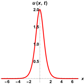
(a) 1-D

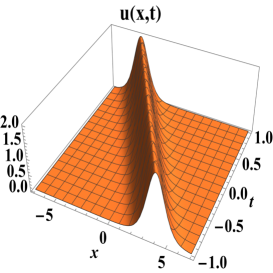
(b) 3-D

Figure 1: (a) represents the one dimensional dynamics of one soliton solution where as in (b) its three dimensional profile has been shown.

3.2 Two-soliton solution $u[2]$

Now the two-fold Darboux transformation with trivial solution u=0 will take the following form

$$u[2]=2\frac{d^{2}}{dx^{2}}\log{[W(\psi_{1},\psi_{2})}],$$ (40)

where

$$u[2]=2\frac{d^{2}}{dx^{2}}\log\begin{vmatrix}\psi_{1}&\psi_{2}\\ \frac{d\psi_{1}}{dx}&\frac{d\psi_{2}}{dx}\end{vmatrix},$$ (41)

We can calculate the value for $\psi_{1}$ and $\psi_{2}$ from the linear system (2) at $\lambda=\lambda_{1}$ and $\lambda=\lambda_{2}$ respectively as below

$$\psi_{1}(x,t)=2\cosh{(k_{1}x+4k_{1}\lambda_{1}t)},$$ (42)

$$\psi_{2}(x,t)=2\sinh{(k_{2}x+4k_{2}\lambda_{2}t)},$$ (43)

After substituting above values into equation (41), we get following results

$$u[2]=2\frac{d^{2}}{dx^{2}}\log\begin{vmatrix}2\cosh(k_{1}x+4k_{1}\lambda_{1}t)&2\sinh(k_{2}x+4k_{2}\lambda_{2}t)\\ 2k_{1}\sinh(k_{1}x+4k_{1}\lambda_{1}t)&2k_{2}\cosh(k_{2}x+4k_{2}\lambda_{2}t)\end{vmatrix},$$ (44)

now expanding the determinate and taking derivations, finally we obtain the following result

$$u[2]=4(k_{2}^{2}-k_{1}^{2})\left[\frac{k_{2}^{2}\cosh(2\gamma_{1})+k_{1}^{2}\cosh(2\gamma_{2})+k_{2}^{2}-k_{1}^{2}}{((k_{2}-k_{1})\cosh{(\gamma_{1}+\gamma_{2})}+(k_{2}+k_{1})\cosh{(\gamma_{1}-\gamma_{2})})^{2}}\right],$$ (45)

which is two-soliton solution well know for KdV equation because KdV equation is embedded as essential part in CNW equation (1) where $\gamma_{1}=k_{1}x+4k_{1}\lambda_{1}t$ and $\gamma_{2}=k_{2}x+4k_{2}\lambda_{2}t$. The inelastic scattering of the two solitons has been visualised in one dimension as well as on plane as below

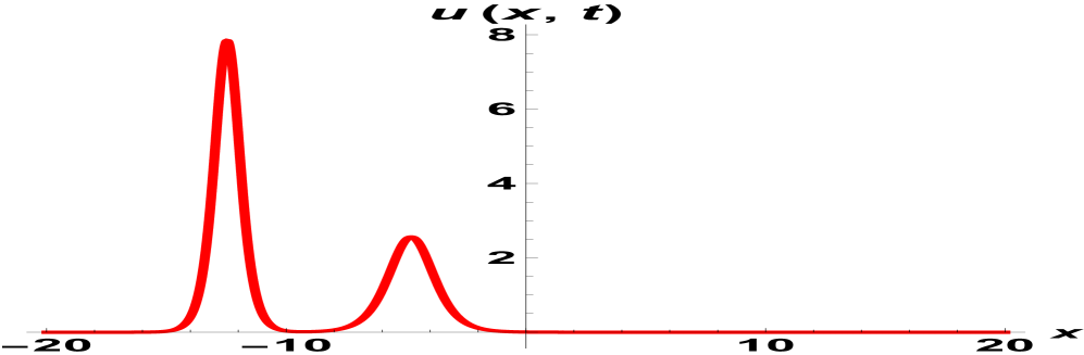
(a) 1-D

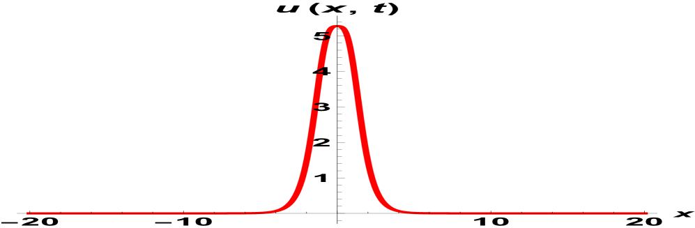
(b) 1-D

Figure 2: (a) represents the one dimensional dynamics of two soliton solution before interaction where as in (b) one dimensional dynamics at the time of interaction has been shown.

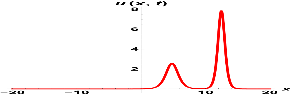
(a) 1-D

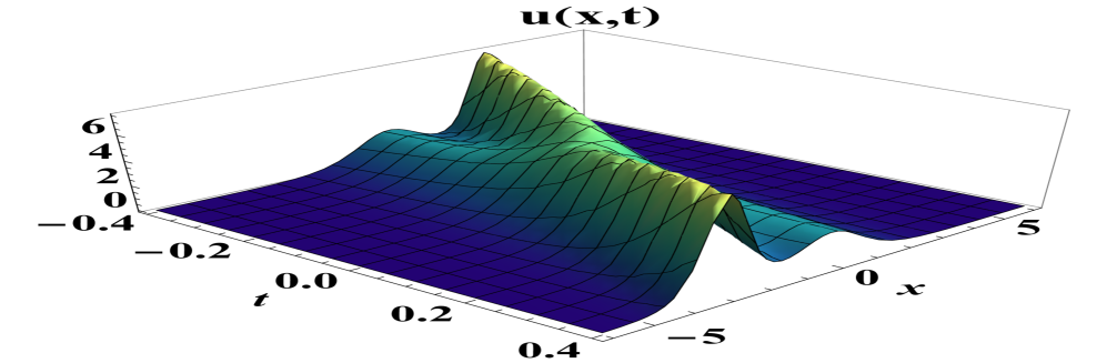
(b) 1-D

Figure 3: (a) represents the one dimensional dynamics of two soliton solution after the interaction where as in (b) three dimensional dynamics of interaction has been shown.

3.3 Two-soliton solution $q[2]$ for coupling variable $v$

In this part of section $2$, we derive two-soliton solution to coupling field variable $v$, as it is obvious from $N$-the expression (LABEL:23) at $N=1$, $q[1]=0$ implies $v[1]=0$, it means at first iteration only KdV solution appears. But the second iteration at $N=2$ yields non zero two soliton solution to coupling field variable $v$ as below

$$q[2]=q[1]-\left(u[1]_{t}-u[1]_{xxx}-6u[1]u[1]_{x}\right)\sigma_{2}[1]^{-1},$$ (46)

Now substitute the calculated values of $u[1]$ and $\sigma_{2}[1]$ in last express (46) and then after simplification, we get

$$q[2]=\frac{\left[16k_{1}^{3}(k_{1}^{2}-\lambda)\operatorname{sech}{\gamma_{1}}^{2}\tanh{\gamma_{1}}(k_{2}\coth{\gamma_{2}}-k_{1}\tanh{\gamma_{1}})\right]}{(k_{1}^{2}-k_{2}^{2})},$$ (47)

this straight forward to obtain $v[2]$ by taking square root of $q[2]$ which is again two-soliton solution. The elastic interaction of these two solitons has been show in one dimension.

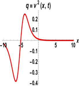
(a) 1-D

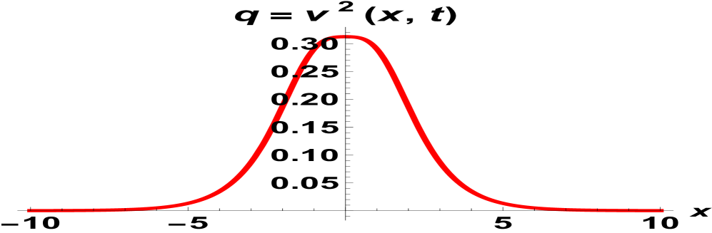
(b) 1-D

Figure 4: (a) represents the one dimensional dynamics of two soliton solution before interaction where as in (b) one dimensional dynamics at the time of interaction has been shown.

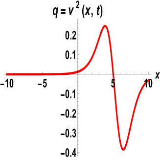
Figure 5: represents the one dimensional dynamics of two soliton solution after the interaction

Here we have calculated two-soliton solutions for the coupling field variables $u$ and $v$ which simultaneously satisfy CNW equation (1). The two-soliton solution $u[2]$ can be assumed as interaction of KdV solitons associated to CNW equation (1), where as $v[2]$ which can be obtained from $q[2]$ also two-soliton solution differs from $u[2]$ associated to same equation (1) that composed by soliton and anti-soliton propagating in opposite directions and interact elastically.

3.4 Three-soliton solution $u[3]$

The three-fold Darboux transformation (21) with trivial solution u=0 will take the following form

$$u[3]=2\frac{d^{2}}{dx^{2}}\log\left[W(\psi_{1},\psi_{2},\psi_{3})\right],$$ (48)

we can compute the value for $\psi_{3}$ form the linear system (2) at $\lambda=\lambda_{3}$ which is given by

$$\psi_{3}(x,t)=2\cosh{(\gamma_{3})}.$$ (49)

with

$$\gamma_{3}=k_{3}x+4k_{3}\lambda_{3}t.$$ (50)

Now after substituting these values in equation (48) and simplifying, we get

$$u[3]=[-(k_{1}k_{3}(-k_{1}^{2}+k_{3}^{2})\sinh{\gamma_{1}}\sinh{\gamma_{2}}\sinh{\gamma_{3}}+k2\cosh{\gamma_{2}}(k1(k1^{2}-k2^{2})\cosh{\gamma_{3}}\\ \sinh{\gamma_{1}}+k3(k2^{2}-k3^{2})\cosh{\gamma_{1}}\sinh{\gamma_{3}}))^{2}+(k1(-k2^{2}+k3^{2})\cosh{\gamma_{3}}\sinh{\gamma_{1}}\sinh{\gamma_{2}}\\ +\cosh{\gamma_{1}}(k2(k1^{2}-k3^{2})\cosh{\gamma_{2}}\cosh{\gamma_{3}}+(-k1^{2}+k2^{2})k3\sinh{\gamma_{2}}\sinh{\gamma_{3}}))\\ (k1(k1^{2}-k2^{2}-k3^{2})(k2^{2}-k3^{2})\cosh{\gamma_{3}}\sinh{\gamma_{1}}\sinh{\gamma_{2}}+\cosh{\gamma_{1}}(-k2(k1^{2}-k3^{2})\\ (-k1^{2}+k2^{2}-k3^{2})\cosh{\gamma_{2}}\cosh{\gamma_{3}}-(k1^{2}-k2^{2})k3(k1^{2}+k2^{2}-k3^{2})\sinh{\gamma_{2}}\sinh{\gamma_{3}}))]\\ /[k_{1}(-k_{2}^{2}+k_{3}^{2})\cosh{\gamma_{3}}\sinh{\gamma_{1}}\sinh{\gamma_{2}}+\cosh{\gamma_{1}}\\ (k_{2}(k_{1}^{2}-k_{3}^{2})\cosh{\gamma_{2}}\cosh{\gamma_{3}}+k_{3}(-k_{1}^{2}+k_{2}^{2})\sinh{\gamma_{2}}\sinh{\gamma_{3}})]^{2},$$ (51)

which is the explicit expression of three-soliton solution for $u$ associated with CNW equation and the interactions of these solitons have been shown below.

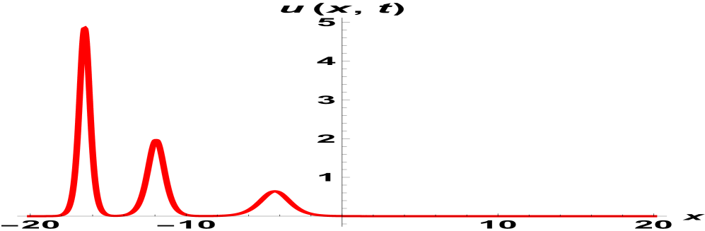
(a) 1-D

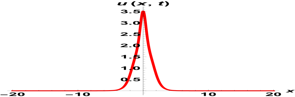
(b) 1-D

Figure 6: (a) represents the one dimensional dynamics of three soliton solution before interaction where as in (b) one dimensional dynamics at the time of interaction has been shown.

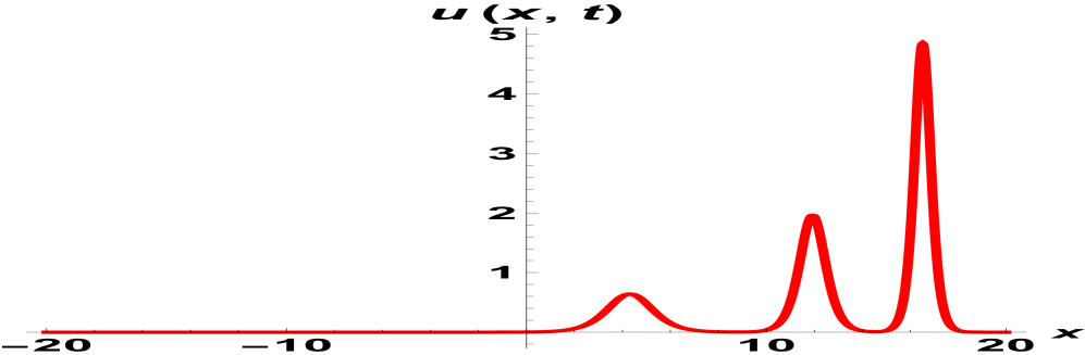
(a) 1-D

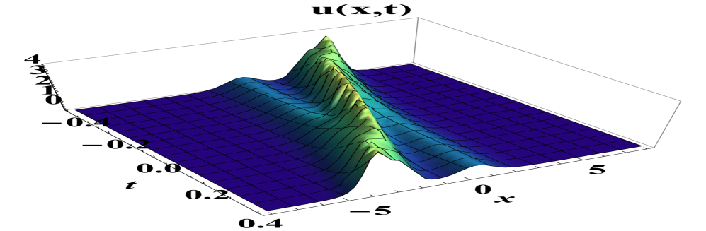
(b) 1-D

Figure 7: (a) represents the one dimensional dynamics of three soliton solution after the interaction where as in (b) representing interaction of three solitons on plane.

3.5 Three-soliton solution $q[3]$ for coupling variable $v$

As above we have derived KdV-type three soliton solution and it seems more substantial to calculate three soliton solution to its coupling partner $v$. For this purpose let write (LABEL:23) at $N=3$ in following form

$$q[3]=q[2]-\left(u[2]_{t}-u[2]_{xxx}-6u[1]u[1]_{x}\right)\sigma_{3}[2]^{-1},$$ (52)

Now substitute the calculated values of $u[2]$ and $\sigma_{3}[2]$ in above expression then after simplification, we get

$$q[3]=q[2]-A*B$$ (53)

where

$$A=(4(k_{1}^{2}-k_{2}^{2})(-\lambda_{2}k_{1}^{2}k_{2}^{2}(k_{1}^{2}-k_{2}^{2})\cosh{\gamma_{1}}(\cosh{\gamma_{1}}+\cosh{\gamma_{2}})\sinh{\gamma_{2}}\\ (k_{2}\cosh{\gamma_{1}}\cosh{\gamma_{2}}-k_{1}\sinh{\gamma_{1}}\sinh{\gamma_{2}})^{2}+4(-k_{1}^{2}+k_{2}^{2}+k_{2}^{2}\cosh{\gamma_{1}}+k_{1}^{2}\cosh{\gamma_{2}})\\ (k_{1}k_{2}(-\lambda_{1}+\lambda_{2})\cosh{\gamma_{2}}\sinh{\gamma_{1}}+(k_{1}^{2}\lambda_{1}-k_{2}^{2}\lambda_{2})\cosh{\gamma_{1}}\sinh{\gamma_{2}})\\ (k_{2}\cosh{\gamma_{1}}\cosh{\gamma_{2}}-k_{1}\sinh{\gamma_{1}}\sinh{\gamma_{2}})^{2}-6k_{1}k_{2}(k_{1}^{2}-k_{2}^{2})\\ (k_{2}\cosh{\gamma_{1}}\cosh{\gamma_{2}}-k_{1}\sinh{\gamma_{1}}\sinh{\gamma_{2}})(1/2\cosh{\gamma_{1}}^{2}(-3k_{1}^{2}+\\ 4k_{2}^{2}+(3k_{1}^{2}-2k_{2}^{2})\cosh{2\gamma_{2}})-k_{1}^{2}\sinh{\gamma_{1}}^{2}\sinh{\gamma_{2}}^{2})(k_{2}\sinh{2\gamma_{1}}+k_{1}\sinh{2\gamma_{2}})\\ +4k_{1}^{2}k_{2}^{2}(-k_{2}\cosh{\gamma_{1}}\cosh{\gamma_{2}}+k_{1}\sinh{\gamma_{1}}\sinh{\gamma_{2}})^{3}(k_{1}\sinh{2\gamma_{1}}+k_{2}\sinh{2\gamma_{2}}+\\ 4k_{1}k_{2}(k_{2}\cosh{\gamma_{1}}\cosh{\gamma_{2}}-k_{1}\sinh{\gamma_{1}}\sinh{\gamma_{2}})^{3}(k_{2}\lambda_{1}\sinh{2\gamma_{1}}+k_{1}\lambda_{2}\sinh{2\gamma_{2}})+\\ (k_{1}^{2}-k_{2}^{2})(k_{1}^{2}-k_{2}^{2}-k_{2}^{2}\cosh{2\gamma_{1}}-k_{1}^{2}\cosh{2\gamma_{2}})(-k_{1}k_{2}\cosh{\gamma_{1}}^{2}\cosh{\gamma_{2}}(-k_{1}^{2}-2k_{2}^{2}+\\ k_{1}^{2}\cosh{2\gamma_{2}})\sinh{\gamma_{1}}+\cosh{\gamma_{1}}^{3}(-6k_{1}^{4}+17k_{1}^{2}k_{2}^{2}-10k_{2}^{4}+(6k_{1}^{4}-7k_{1}^{2}k_{2}^{2}+2k_{2}^{4})\cosh{2\gamma_{2}})\\ \sinh{\gamma_{2}}-k_{1}^{2}\cosh{\gamma_{1}}(-4k_{1}^{2}+7k_{2}^{2}+(4k_{1}^{2}-3k_{2}^{2})\cosh{2\gamma_{2}})\sinh{\gamma_{1}}^{2}\sinh{\gamma_{2}}+\\ k_{1}^{3}k_{2}\sinh{\gamma_{1}}^{3}\sinh{\gamma_{2}}\sinh{2\gamma_{2}})+6(k_{1}^{2}-k_{2}^{2})(k_{1}^{2}-k_{2}^{2}-k_{2}^{2}\cosh{2\gamma_{1}}-k_{1}^{2}\cosh{2\gamma_{2}})\\ (-2(k_{1}^{2}-k_{2}^{2})\cosh{\gamma_{1}}(-k_{1}^{2}+k_{2}^{2}+k_{2}^{2}\cosh{2\gamma_{1}}+k_{1}^{2}\cosh{2\gamma_{2}})\sinh{\gamma_{2}}+2k_{1}k_{2}\\ (-k_{2}\cosh{\gamma_{1}}\cosh{\gamma_{2}}+k_{1}\sinh{\gamma_{1}}\sinh{\gamma_{2}})(k_{2}\sinh{2\gamma_{1}}+k_{1}\sinh{2\gamma_{2}}))))\\ /(k_{2}\cosh{\gamma_{1}}\cosh{\gamma_{2}}-k_{1}\sinh{\gamma_{1}}\sinh{\gamma_{2}})^{5},$$ (54)

$$B=(k_{1}(-k_{2}^{2}+k_{3}^{2})\cosh{\gamma_{3}}\sinh{\gamma_{1}}\sinh{\gamma_{2}}+\cosh{\gamma_{1}}(k_{2}(k_{1}^{2}-k_{3}^{2})\cosh{\gamma_{2}}\cosh{\gamma_{3}}\\ +(-k_{1}^{2}+k_{2}^{2})k_{3}\sinh{\gamma_{2}}\sinh{\gamma_{3}}))/(k_{1}k_{3}(-k_{1}^{2}+k_{3}^{2})\sinh{\gamma_{1}}\sinh{\gamma_{2}}\sinh{\gamma_{3}}+\\ k_{2}\cosh{\gamma_{2}}(k_{1}(k_{1}^{2}-k_{2}^{2})\cosh{\gamma_{3}}\sinh{\gamma_{1}}+k_{3}(k_{2}^{2}-k_{3}^{2})\cosh{\gamma_{1}}\sinh{\gamma_{3}})),$$ (55)

this is straight forward to obtain $v[3]$ by taking square root of $q[3]$ and we have shown three soliton elastic interaction in one dimension.

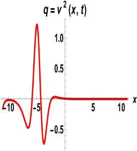
(a) 1-D

(b) 1-D

Figure 8: (a) represents the one dimensional dynamics of three soliton solution before interaction where as in (b) one dimensional dynamics at the time of interaction has been shown.

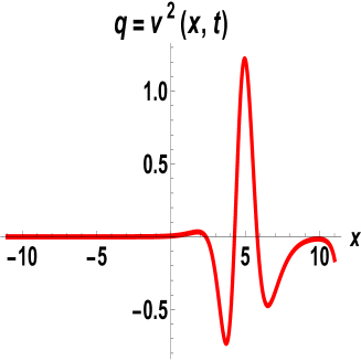
Figure 9: represents the one dimensional dynamics of three soliton solution after the interaction

As in above last section, we derived three-soliton solutions for the coupling field variables $u$ and $v$ which simultaneously satisfy CNW equation (1). The three-soliton solution $u[3]$ can be assumed as interaction of KdV solitons associated to CNW equation (1), where as $v[3]$ which can be obtained from $q[3]$ also three-soliton solution differs from $u[3]$ associated to same equation (1) that composed by soliton and anti-soliton propagating in opposite directions and interact elastically.

4 Equation of Continuity and conserved densities

This section is devoted to construct the equation of continuity which is associated with CNW equation (1) and derivation of conserved densities incorporating its riccati equation.
For this purpose, let define a quantity $\Gamma$ in terms of arbitrary function, as below

$$\Gamma=\frac{\psi^{\prime}}{\psi}=(ln\psi)_{x},$$ (56)

Now take the time derivative of $\Gamma$ and then make use of equation (3) in resulting expression, we get folowing result after simplification

$$\frac{\partial\Gamma}{\partial t}=2u^{\prime}\Gamma+\left(4\lambda+2u\right)\left(\frac{\psi^{\prime\prime}}{\psi}-\frac{{\psi^{\prime}}^{2}}{\psi^{2}}\right)-u^{\prime\prime},$$ (57)

and the space derivative of equation(56) can be written as

$$\frac{\partial\Gamma}{\partial x}=\frac{\psi^{\prime\prime}}{\psi}-\frac{{\psi^{\prime}}^{2}}{\psi^{2}},$$ (58)

Now eliminating $\left(\frac{\psi^{\prime\prime}}{\psi}-\frac{{\psi^{\prime}}^{2}}{\psi^{2}}\right)$ from equation (57), and by using last equation equation(58), after simplification we obtain resulting expression as below

$$\frac{\partial\Gamma}{\partial t}=\frac{\partial}{\partial x}\left[(4\lambda+2u)\Gamma-u^{\prime}\right],$$ (59)

or

$$\frac{\partial\rho}{\partial t}-\frac{\partial J}{\partial x}=0$$ (60)

the above is the equation of continuity associated with CNW equation (1) involving density as $\rho$ and corresponding current as $j$ given as

$$J=(4\lambda+2u)\Gamma-u^{\prime}.$$ (61)

We may construct the hierarchy of conserved densities for CNW equation (1) with the help of its riccati equation as calculated below.
It is straight forward to construct the riccati equation from expression (58) by using equation (2) as in the following form

$$\frac{\partial\Gamma}{\partial x}+\left(u-\lambda+\frac{q}{4\lambda}\right)+\Gamma^{2}=0,$$ (62)

Now by taking the derivation of above Riccati equation with respect $x$, we obtain second order ordinary differential equation as

$$\frac{\partial^{2}\Gamma}{\partial x^{2}}-2\Gamma^{3}+2\Gamma\left(\lambda-u-\frac{q}{4\lambda}\right)+u^{\prime}+\frac{q^{\prime}}{4\lambda}=0.$$ (63)

Let consider following ansatz as the solution of above equation

$$\Gamma=\sum_{n=1}^{\infty}\Gamma_{n}\lambda^{-n},$$ (64)

where the quantities $\Gamma_{n}$ are to be determined which represent the densities associated with Ito type coupled equation (1). After substituting ansatz (64) into equation(63) and then expanding summation, finally the coefficients of $\lambda^{0}$, $\lambda^{-1}$ , $\lambda^{-2}$ in resulting expression produce first three densities

$$\Gamma_{1}=-\frac{u^{\prime}}{2},$$ (65)

$$\Gamma_{2}=\frac{u^{\prime\prime\prime}}{4}-\frac{q^{\prime}}{8}-\frac{1}{2}uu^{\prime},$$ (66)

$$\Gamma_{3}=u\Gamma_{2}+\frac{q}{4}\Gamma_{1}-\frac{1}{2}\frac{\partial^{2}}{\partial x^{2}}\Gamma_{2}.$$ (67)

and the coefficients of $N$-the terms yield the following relation

$$\Gamma_{n+1}=\frac{1}{2}\left[2u\Gamma_{n}+\frac{q}{2}\Gamma_{n-1}+2\sum_{l=1}^{m=n-2}\Gamma_{l}\left(\sum_{k=1}^{j=m-l+1}\Gamma_{k}\Gamma_{j-k+1}\right)-\frac{\partial^{2}}{\partial x^{2}}\Gamma_{n}\right],$$ (68)

which holds for $n=3,4,5,...,$ and with the help of that expression we may calculate all remaining conserved densities. Now we can expression (58) can be written in $n$-th form $J_{n}=(4\lambda+2u)\Gamma_{n}-u^{\prime}$that yields the corresponding currents.

5 Conclusion

In this article, we have calculated multi-solitonic solutions for coupling field variables $u$, $q$ associted with Ito type coupled KdV equation (1) in Darboux framework and then their $N$-fold Darboux transformations generalised in terms of Wronkians. We also derived its equation of continuity with hierarchy of conserved densities. For motivation, It is quite interesting to construct its Hirota bilinear form with multi-solitoinc solutions and comparable to our results obtained here, that will be discussed in a separate paper. Further, it is straight forward to calculate its noncommutative analogue with $N$-fold Darboux solutions in terms of quasideterminats which may coincide with our results under commutative limit.

6 Acknowledgement

This research work has been completed as the part of Belt and Road Young Scientist project sponsored by Science and technology commission of Shanghai at college of science, Shanghai University with project, No. $20590742900$. We are also thankful to the Punjab University 54590 on providing me the facilities to complete that work.

References

-
[1]
N.J. Zabusky, C.J. Galvin, Shallow-water waves, the Korteweg-deVries equation and solitons, J. Fluid Mech. 47 (1971) 811–824
https://doi.org/10.1017/S0022112071001393 -
[2]
A.H. Khater, D.K. Callebaut, A.R. Seadawy, General soliton solutions for nonlinear dispersive waves in convective type instabilities, Phys. Scr. 74 (2006) 384–393.
https://doi.org/10.1088/0031-8949/74/3/015 -
[3]
Y. V. Kartashov, B.A. Malomed, L. Torner, Solitons in nonlinear lattices, Rev. Mod. Phys. 83 (2011) 247–305.
https://doi.org/10.1103/RevModPhys.83.247 -
[4]
D.-S. Wang, X.-F. Zhang, P. Zhang, W.M. Liu, Matter-wave solitons of Bose–Einstein condensates in a time-dependent complicated potential, J. Phys. B At. Mol. Opt. Phys. 42 (2009) 245303.
https://doi.org/10.1088/0953-4075/42/24/245303 -
[5]
D.-S. Wang, S.-W. Song, B. Xiong, W.M. Liu, Quantized vortices in a rotating Bose-Einstein condensate with spatiotemporally modulated interaction, Phys. Rev. A. 84 (2011) 053607.
https://doi.org/10.1103/PhysRevA.84.053607 -
[6]
Y. V. Kartashov, V.A. Vysloukh, L. Torner, Surface Gap Solitons, Phys. Rev. Lett. 96 (2006) 073901.
https://doi.org/10.1103/PhysRevLett.96.073901 -
[7]
M. Ito, Symmetries and conservation laws of a coupled nonlinear wave equation, Phys. Lett. A. 91 (1982) 335–338.
https://doi.org/10.1016/0375-9601(82)90426-1 -
[8]
H.M. Baskonus, M. Kayan, Regarding new wave distributions of the non-linear integro-partial Ito differential and fifth-order integrable equations, Appl. Math. Nonlinear Sci. (2021).
https://doi.org/10.2478/amns.2021.1.00006 -
[9]
V.B. Matveev, M. A. Salle, Darboux Transformations and Solitons, Springer Berlin Heidelberg, Berlin, Heidelberg, 1991.
https://doi.org/10.1007/978-3-662-00922-2 -
[10]
C. Gu, H. Hu, Z. Zhou, Darboux Transformations in Integrable Systems, Springer Netherlands, Dordrecht, 2005.
https://doi.org/10.1007/1-4020-3088-6 -
[11]
A. Trisetyarso, Application of Darboux Transformation to solve Multisoliton Solution on Non-linear Schrödinger Equation, (2009).
http://arxiv.org/abs/0910.0901 -
[12]
A. Trisetyarso, Correlation of Dirac potentials and atomic inversion in cavity quantum electrodynamics, J. Math. Phys. 51 (2010) 072103.
https://doi.org/10.1063/1.3458598 -
[13]
A. Trisetyarso, Dirac four-potential tunings-based quantum transistor utilizing the Lorentz force, (2010).
http://arxiv.org/abs/1003.4590 -
[14]
M. Irfan, Lax pair representation and Darboux transformation of noncommutative Painlevé’s second equation, J. Geom. Phys. 62 (2012) 1575–1582.
https://doi.org/10.1016/j.geomphys.2012.01.008 -
[15]
I. Mahmood, Quasideterminant solutions of NC Painlevé II equation with the Toda solution as a seed solution in its Darboux transformation, J. Geom. Phys. 95 (2015) 127–136.
https://doi.org/10.1016/j.geomphys.2015.05.004 -
[16]
M. Hassan, Darboux transformation of the generalized coupled dispersionless integrable system, J. Phys. A Math. Theor. 42 (2009) 065203.
https://doi.org/10.1088/1751-8113/42/6/065203 -
[17]
M.J. Ablowitz, D.J. Kaup, A.C. Newell, H. Segur, The Inverse Scattering Transform-Fourier Analysis for Nonlinear Problems, Stud. Appl. Math. 53(1974) 249–315.
https://doi.org/10.1002/sapm1974534249 - [18] A. B. Shabat, V. E. Adler, V. G. Marikhin, and V. V. Sokolov. Encyclopedia of integrable systems. LDLandau Institute for Theoretical Physics, 303:68, 2010..
-
[19]
Y. Kai, J. Ji, Z. Yin, Exact solutions and dynamic properties of Ito-Type coupled nonlinear wave equations, Phys. Lett. A. 421 (2022) 127780.
https://doi.org/10.1016/j.physleta.2021.127780 -
[20]
V. B. Matveev, Generalized Wronskian formula for solutions
of the KdV equations: first applications, Phys. Lett. A. 166 (1992) 205-208.
https://doi.org/10.1016/0375-9601(92)90362-P - [21] Q. H. Park and H. J. Shin, Darboux transformation and Crum’s formula for multi-component integrable equations, Physica D 157 (2001) 1–15. https://doi.org/10.1016/S0167-2789(01)00292-5