Finding Label and Model Errors in Perception Data With Learned Observation Assertions

Abstract.

ML is being deployed in complex, real-world scenarios where errors have impactful consequences. In these systems, thorough testing of the ML pipelines is critical. A key component in ML deployment pipelines is the curation of labeled training data. Common practice in the ML literature assumes that labels are the ground truth. However, in our experience in a large autonomous vehicle development center, we have found that vendors can often provide erroneous labels, which can lead to downstream safety risks in trained models.

To address these issues, we propose a new abstraction, learned observation assertions, and implement it in a system called Fixy. Fixy leverages existing organizational resources, such as existing (possibly noisy) labeled datasets or previously trained ML models, to learn a probabilistic model for finding errors in human- or model-generated labels. Given user-provided features and these existing resources, Fixy learns feature distributions that specify likely and unlikely values (e.g., that a speed of 30mph is likely but 300mph is unlikely). It then uses these feature distributions to score labels for potential errors. We show that Fixy can automatically rank potential errors in real datasets with up to 2$\times$ higher precision compared to recent work on model assertions and standard techniques such as uncertainty sampling.

1. Introduction

Machine learning (ML) is increasingly being deployed in complex applications with real-world consequences. For example, ML models are being deployed to make predictions over perception data in autonomous vehicles (AVs) (Kaparthy, 2018), with potentially fatal consequences for errors, such as striking pedestrians (Wakabayashi, 2018). Thus, quality assurance and testing of ML pipelines are of paramount concern (Zhang et al., 2020; Amershi et al., 2019; Odena et al., 2019; Xiang et al., 2018).

A critical component of ML deployments is the curation of high-quality training data, in which crowd workers produce labels over data. Similar to how errors in tabular data results in downstream errors in query results, erroneous training data (e.g., Figure 1) can lead to subsequent safety repercussions for trained models. As such, finding these errors is critical, which we focus on in this work.

Unfortunately, standard techniques in data cleaning are not well suited for finding errors in training data. For example, while constraints work well on tabular data, they are less suited for perception data, e.g., pixels of an image. As such, we have found it necessary to develop new tools for finding errors in training data.

Figure 1. Example of human labels (orange) and missing labels (red) in the Lyft Perception dataset. The black truck highlighted is within 25m of the AV. Such errors can cause downstream issues with perception and planning systems.

Recent work has proposed Model Assertions (MAs) that indicate when errors in ML model predictions or labels may be occurring (Kang et al., 2020). MAs are black-box functions over model inputs and outputs that return a quantitative severity score indicating when an ML model or human-proposed label may have an error. For example, a MA may assert that a prediction of a box of a car should not appear and disappear in subsequent frames of a video. MAs can be used to monitor the ML models in deployment, and to flag problematic data to label and retrain the model.

However, in our experience deploying MAs in a real-world AV perception training pipeline, we have found several major challenges. First, users must manually specify MAs, which can be challenging for complex ML deployments. Second, calibrating severity scores so that higher severity scores indicate a higher chance of error is challenging. This is especially important as organizations have limited resources to evaluate potential errors in ML models or human labels. Third, ad-hoc methods of specifying severity scores ignores organizational resources (Suri et al., 2020) that are already present: large amounts of ground-truth labels and existing ML models.

To address these challenges, we propose a probabilistic domain-specific language (DSL), Learned Observation Assertions (LOA), for specifying assertions, and methods for data-driven specification of severity scores that leverage existing resources in ML deployments. We implement LOA in a prototype system (Fixy), embedded in Python to easily integrate with ML systems.

Our first contribution, LOA, allows users to specify properties of interest for perception tasks. LOA contains three components: data associations, feature distributions, and application objective functions. LOA can be used to specify assertions without ad-hoc code or severity scores by automatically transforming the specification into a probabilistic graphical model and scoring data components, producing statistically grounded severity scores.

In our labeling deployment, sensor data across short snippets of time (scenes) are sent to vendors for labeling. These scenes are then audited for missing labels. These errors are difficult to specify via ad-hoc MAs, so our DSL supports means of associating observations together: across observation sources (observation bundles, i.e., predictions from different ML models or sensors) and across time (tracks, i.e., predictions of the same object over time). These associated observations can then be considered jointly when searching for errors.

Our second contribution is methods of leveraging organizational resources (Suri et al., 2020), i.e., existing labels and ML models, to automatically specify severity scores via LOA. Users specify features over data, which are used to automatically generate feature distributions, and application objective functions (AOFs) to guide the search for errors. Feature distributions take sets of observations and output a probability of seeing a feature of the input. For example, a feature distribution might take a 3D bounding box of a car and return the likelihood of encountering that box volume. AOFs transform feature distribution values for the application at hand. For example, if we wish to find likely tracks (e.g., a track missed by human labels), the AOF could simply return the feature distributions’ value. If we wish to find unlikely tracks (e.g., a “ghost” track that an ML model erroneously predicts), the AOF could return one minus the feature distributions’ value.

We evaluate Fixy on two real-world AV datasets, the publicly available Lyft Level 5 perception dataset (Kesten et al., 2019) as well as an internally collected dataset. Both datasets were annotated by leading commercial labeling vendors. Despite best efforts from these vendors (Cheng, 2019), we find a number of labeling errors via Fixy, some of which could cause safety violations (e.g., in Figures 1 and 8). We first show that Fixy can achieve recalls of up to 75% when searching for errors in these datasets, while achieving 2$\times$ higher precision for finding label error than hand-crafted MAs. Furthermore, Fixy can find novel errors in ML models that the hand-crafted MAs in previous work are unable to find, and finds high-confidence errors that uncertainty sampling misses.

In summary, our contributions are

1. LOA, a probabilistic DSL with syntax and semantics for validating observations over complex perception data.

2. Methods for leveraging organizational resources (in the form of existing ML models and labels) to automatically tune feature distributions and detect errors.

3. An empirical evaluation of our implementation Fixy, showing it can outperform baselines for detecting errors even in commercially generated and vetted label data.

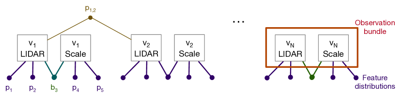
(a) Schematic of a track that contains observations from LIDAR ML model predictions and from human-proposed labels. We show examples of feature distributions for observations ($p_{1}$, $p_{2}$, $p_{4}$, and $p_{5}$), bundles ($b_{3}$), and transitions ($p_{1,2}$).

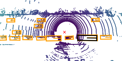
(b) $t=1$ ($v_{1}$ model and $v_{1}$ human)

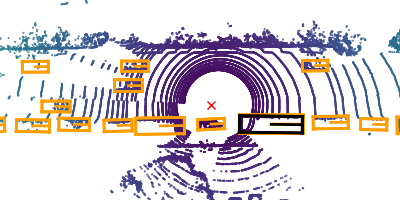
(c) $t=2$ ($v_{2}$ model and $v_{2}$ human)

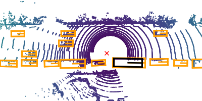
(d) $t=3$ ($v_{3}$ model and $v_{3}$ human)

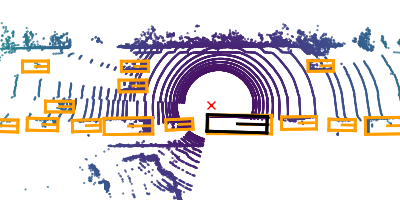
(e) $t=4$ ($v_{4}$ model and $v_{4}$ human)

Figure 2. Example of the factor graph (top) and corresponding LIDAR point cloud data (bottom). We show here and throughout the birds eye view of the LIDAR frame. Concentric circles represent equidistance from the sensor. Reflected points from objects are shown as dots. The track is in black and other human-proposed labels are in orange for reference.

2. Example and Background

ML workflow. As an example, we describe the ML deployment pipeline for our AVs, focusing on labeling data for perception systems. Other organizations deploy similar pipelines, e.g., as documented by Kaparthy (2018).

Our AV deployment pipeline is a continuous process, in which ML models are trained, tested, and deployed on vehicles. Because ML models are continuously exposed to new and different scenarios, we continuously collect and label data, which is subsequently used to develop and retrain ML models (Baylor et al., 2017).

Label quality is of paramount concern: erroneous labels can lead to downstream errors, which in turn can lead to safety violations. Vendors that provide labels are not always accurate, which is in contrast to the large body of work that assumes datasets are “gold.” For our perception system, the most egregious errors are when objects are entirely missed in labeling. We show examples of missing labels in Figure 1, in which a truck and several cars were missed by the human labeler.

To address label quality issues, our organization has expert auditors who audit the vendor-provided labels. Unfortunately, it is too expensive to audit every data point, so we have developed Fixy, which enables ranking datapoints that are likely to be erroneous and allows better utilization of auditing resources.

Model assertions. MAs are user-provided, black box functions over ML model inputs and outputs that indicate if the ML model has an error (Kang et al., 2020). MAs can be deployed at test time to indicate possible errors so corrective actions can be taken. They can additionally be used to select data that produces errors for labeling, e.g., as studied by Kang et al. (2020), as many organizations continuously collect data to label.

Unfortunately, MAs are specified in an ad-hoc manner. They require users to write programs to specify exactly what forms of errors occur and ad-hoc severity scores to indicate the likelihood of an error. We have found that these ad-hoc procedures can be challenging to use.

Factor graphs. Fixy generates graphical models from data and feature distributions. We specifically consider factor graphs due to the ease of representing data and distributions (Kschischang et al., 2001).

Given a set of random variables $X=\{X_{1},\dots,X_{n}\}$, a factor graph represents a factorization of a joint distribution $g(X_{1},\dots,X_{n})$. Assume that the joint distribution can be factorized in terms of a set of functions $f_{j}$, which we will call factors, and $S_{j}\subseteq X$

(1) $$g(X_{1},...,X_{n})=\prod_{j=1}^{m}f_{j}(S_{j}).$$

Formally, we can represent a factor graph as a graph $G=(X,F,E)$, where $X$ and $F$ are two disjoint sets of nodes. The graph is bipartite, meaning that each edge connects a node in $X$ to a node in $F$, but no edge connects nodes in $X$ among themselves nor nodes in $F$ among themselves. For every factor $f_{j}\in F$, there is an edge that connects it to $X_{i}$ if and only if $X_{i}\in S_{j}$ in the factorization of $g$.

We consider specific factor graphs that are automatically generated by Fixy, as described later in this paper.

LIDAR. We extensively use and show LIDAR data and predictions over LIDAR data as examples of missing human labels or ML model predictions. LIDAR is generated by pulsing light and timing the returns of the pulsed light (Wandinger, 2005). With accurate timings, LIDAR data gives accurate distance measurements and are represented as point clouds. In this paper, we show birds-eye view of LIDAR data: concentric circles indicate same distances from the LIDAR sensor and we draw predicted boxes over the scenes. We show an example in Figure 2. LIDAR figures in white background are from the Lyft Level 5 perception dataset (Kesten et al., 2019) and figures in black background are from our internal dataset.

3. System Overview

Goals. Fixy aims to enable users to find errors in ML labeling pipelines and in ML models, primarily in the form of missing labels. In particular, Fixy aims to reduce manual effort by only requiring users to specify natural quantities (e.g., box volume, velocity) as opposed to specifying the exact form of errors as model assertions expect users to do.

Inputs and outputs. We first denote human-proposed labels and ML model outputs as “observations.” As input, Fixy takes a set of observations. As output, Fixy returns a ranked list of (potentially a subset of) observations, where higher ranked observations are ideally more likely to contain errors.

Offline, Fixy takes already-present labels to learn feature distributions over features of the observations. Fixy will then use this data to rank potential errors.

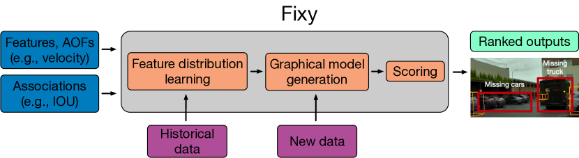
Figure 3. System diagram for Fixy. Users provide features over perception data (e.g., box volume) and associations between observations. Given these inputs, Fixy will learn feature distributions, generate graphical models, score new data, and output potential errors.

Fixy components. Fixy consists of: a DSL for specifying relations between observations and feature distributions, a component to learn feature distributions, a scoring component, and a runtime engine. Fixy’s DSL allows users to specify how feature distributions and observations interact. Its distribution learning component fits distributions over existing observations. Its scoring component scores observations or groups of observations by likelihood. Finally, its runtime engine ranks observations or groups of observations.

We show a system diagram in Figure 3. Users need only provide the features (and data to be ranked). Once the feature distributions are learned, Fixy will rank potential errors for auditing.

Workflow. Fixy contains an offline (distribution learning) and online (error ranking) phase. In the offline phase, Fixy will take existing organizational resources in the form of existing labels to learn feature distributions. In the online phase, Fixy will rank potential errors.

We have found that users of label checking tools are often non-experts in coding and ML tools, so we have opted for simplicity in LOA. Thus, a user of Fixy need only specify features and optionally AOFs. In particular, many features are already computed for use in other pipelines so can be reused (e.g., object volume, velocity, and distance from vehicle). Thus, the features can be specified in few lines of code, as we show below.

Worked example. Consider the use case of finding missing human labels of 3D bounding boxes over LIDAR point cloud data. For example, Figure 1 show several missing cars and a missing truck.

In this example, we have two sources of observations: predictions from an ML model and human labels. To find these errors, the user will: 1) associate observations and 2) specify features. Then, Fixy will automatically score and rank potential errors.

The analyst first associates observations within a time step (i.e., overlapping model predictions and human labels) and between adjacent timesteps (i.e., objects across time). To do so, the user can specify that observations with high box overlap are associated. While this is provided by default by Fixy, the user can also write a short amount of code using the intersection over union (IOU):

⬇

class TrackBundler(Bundler):

def is_associated(self, box1, box2):

return compute_iou(box1, box2) > 0.5

The analyst then specifies features. As a concrete example, the analyst may specify a feature that computes box volume. The user need only provide code to compute the box volume: Fixy will learn distribution of box volumes and use it to find anomalous boxes.

⬇

# KDEObsDistribution takes features and learns a

# KDE density estimator over the features

class VolumeDistribution(KDEObsDistribution):

def feature(self, box):

vol = box.width * box.height * box.length

return vol

The user can also specify other features, such as object velocity. The two code snippets above (and another other features the user wishes to specify) are all that a user need to provide to Fixy.

Given the associations between observations and the features, Fixy will learn the likelihood of encountering specific feature values offline, using already-collected resources.

Once these feature distributions are learned, Fixy will score and rank new data, ideally with potential errors ranked higher. Concretely, consider Figure 1. Although not shown, an ML model highlighted the truck in a time-consistent way. Since the track is highly consistent, Fixy returns a high likelihood of an error. An expert auditor can then verify if the potential error is actually a missing label.

4. Learned Observation Assertions

The LOA DSL provides a simple means of specifying associations between observations and specifying associations between observations and feature distributions. Intuitively, applications that contain observations over time and over multiple modalities/models may have observations that are associated across time/modalities. Furthermore, feature distributions may operate over individual observations or groups of observations. We show an example of a compiled LOA graph and corresponding sensor data observations in Figure 2.

In this section, we provide a formal description of LOA. However, users interface with LOA via a Python library. In particular, users only need to specify features over which distributions are learned and methods of associating observations. Our implementation provides class interfaces where users can override the feature computation (for the feature distributions) and the association method (for associating observations). We show an example in Section 3 of the code the user needs to provide.

4.1. Overview

LOA contains elements for allowing users to specify how observations interact with each other and how feature distributions interact with observations. Our implementation of LOA is embedded in Python for ease of integration with standard ML packages. Since perception data often contains spatial and temporal components, we allow users to construct observation bundles within a single time step and tracks across time. We collectively refer to observations, bundles, and tracks as OBTs. LOA then allows features to be specified over any OBT. Finally, the user can specify application objective functions (AOFs) over any feature distribution.

4.2. Scene Syntax

Overview. We consider scenes of data, which consists of observations and features over these observations. Our syntax consists of specifying how observations relate to each other within a scene and how features relate to groups of observations.

Formalism. A scene consists of a set of tracks. Each track contains a set of observation bundles. An observation bundle contains observations from different modalities, such as LIDAR, vision, and for offline data, human proposals of labels. We summarize our syntax notation in Table 1.

Formally, we denote the scene (i.e., set of tracks) as $s=\{\tau\}$. Each track consists of an indexed sequence of observation bundles, $\tau=(\beta_{0},\dots,\beta_{n})$. Each observation bundle consists of a set of observations, $\beta=\{\omega_{\tau,\beta}\}$.

In order to reason about erroneous or unusual artifacts in the perception system, we define features over the elements of the scene. Users can assign features to any of the elements of the scene; these assignments are often done automatically (e.g., a volume feature would apply over every observation). Concretely, features can be over observations, observation bundles, tracks, or entire scenes.

Formally, $\pi$, the feature function, maps each element to its features. For example, $\pi(\omega_{\tau,\beta})$ are the features assigned to the observation in track $\tau$ in bundle $\beta$, which could be a feature on the volume of the object detected. Similarly, $\pi(\tau)$ assigns track $\tau$ its features, which could be the total number of observations within that track.

In addition to features over discrete groups of observations, we provide syntax for features over adjacent observations within a track (“transition features”), i.e., $\pi(\beta_{i},\beta_{i+1})$. As a concrete example, we have implemented a transition feature for the estimated instantaneous velocity. We note that this syntax is for convenience, as it could be implemented via track features. Nonetheless, we have found it useful in our applications to allow for transition features.

Finally, AOFs can be specified over any feature distribution. These AOFs are numeric transformations of the returned feature distribution score, e.g., the identity function, the zero function, or $f(x)=1-x$.

4.3. Generating Graphical Models

Fixy will compile the scene, feature distributions, and AOFs to a graphical model, which is used to score groups of observations. Fixy uses these scores to flag potential errors.

To compile a scene, Fixy will create nodes for each observation and feature distribution. Then, Fixy will create edges between each feature distribution and the observation it applies over. If a feature distribution applies to a single observation, Fixy will create a single edge. If a feature distribution applies to a group of observations (e.g., an observation bundle or track), Fixy will create one edge between each observation in the group and the feature distribution.

Once the graphical model is constructed, Fixy can then score any OBT. Fixy will score an observation by the negative log-likelihood implied by its feature distributions. The score of a group of observations is the sum of the scores of the observations, normalized by the number of feature distributions. We defer the full discussion of scoring and a worked example to Section 6.

Syntactic element	Meaning
$s$	Scene
$\tau$	Track
$\beta$	Observation bundle
$\omega$	Observation
$\pi$	Feature mapping function

Table 1. Table of syntactic elements in Fixy’s DSL.

5. Feature Distributions

A key component to scoring OBTs are the feature distributions. Both our AV deployment and other organizations deploying ML collect large amounts of training data. This training data contains labels (potentially with errors), which can be used to fit empirical distributions to the features. We leverage these existing labels in this work, as they come at no additional cost.

To fit these feature distributions, Fixy takes as input scalar or vector valued features over OBTs. For example, a feature over an observation may take a bounding box and return the volume of the box as described in Section 3. The user may also manually specify feature distributions to rank severity (e.g., distance of an object to the AV) or to filter certain instances (e.g., only search for errors in detecting pedestrians). Finally, Fixy takes an optional AOF, which can be applied per feature or over the resulting score.

We describe the feature types, their specification, and how Fixy fits them below.

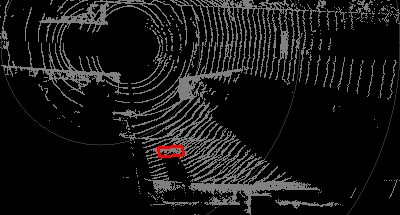
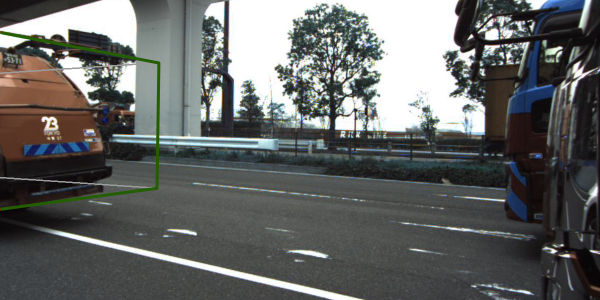
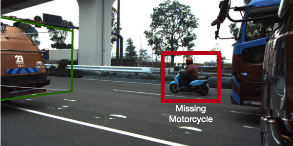
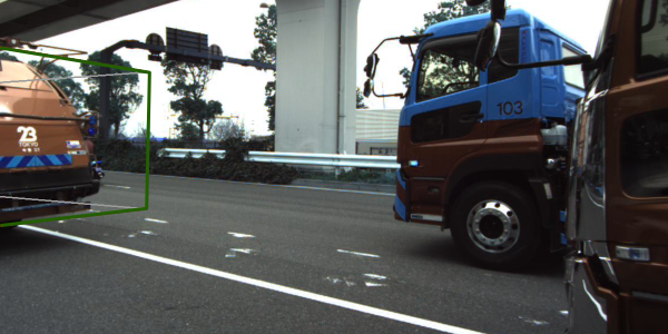
Figure 4. Example of a motorcycle (highlighted in red) missed by human proposals. We show both the LIDAR point cloud data (top) and the camera view (bottom). The motorcycle is occluded by other vehicles, so only appears for a short period of time (<1 second). Nonetheless, it is close to the AV and is thus important to predict.

5.1. Feature Types

Fixy contains features over OBTs and transitions. While transition features can be implemented as track features, we provide a syntactic element for ease of use.

Fixy’s first feature type are features over single observations. Each feature is associated with a specific observation type (e.g., a feature over a LIDAR model prediction). These features are typically used to specify time-independent information over the predictions. For example, a feature may take a 3D box prediction from a LIDAR model and return the box volume. The observation feature would be over box volumes in this case.

Fixy’s second feature type are features over observation bundles. These features are typically used to specify consistency between observations of the same object in a single time step. For example, consider the intuition that observations within bundles should agree on object class. To specify this, a user could provide a feature that returns 0 if all the classes agree and 1 otherwise. The feature would then learn the Bernoulli probability of the class agreement between observation types.

Fixy’s third feature type are features between observations or bundles in adjacent time steps within a track. These features are typically used to specify information over time-dependent quantities or consistency. For example, a feature could specify the velocity estimated by box center offset.

Fixy’s fourth feature type are features over entire tracks. Although rare, these features can be used to normalize scores over entire tracks.

5.2. Learning Feature Distributions

Given features, Fixy can automatically fit feature distributions over existing training datasets. To fit feature distributions, Fixy takes a function that accepts a list of scalars/vectors and returns a fitted distribution. By default, Fixy uses a kernel density estimator (KDE) to learn feature distributions over the features. In some cases, other types of distributions are appropriate (e.g., discrete distributions): the user can override our default KDE estimator in these cases.

To learn feature distributions given a set of scenes, Fixy first exhaustively generates the features over the data and collects the scalar or vector values. Then, for each feature, Fixy executes the fitting function over the scalar/vector values.

We note the density estimators have hyperparameters. We have found that default hyperparameters work in all cases we tried, so we defer exploring hyperparameters to future work.

5.3. Application Objective Functions

AOFs wrap data feature distributions to transform them into an application-specific probabilities to guide the search for labeling errors. As such, they take scalar values and return scalar values. The most common operations are taking the inverse and setting the probability to 0/1 under certain conditions. For example, when searching for likely tracks, the application objective function may be the identity. In contrast, when searching for unlikely tracks, the application objective function may invert the probability.

6. Scoring Relative Plausibility

Given the compiled factor graph, Fixy can score any OBT. Fixy will first score the observations via the sum of log likelihood of the feature distributions transformed by the application objective functions. Formally, given the AOFs $f_{i}$, the score for an observation $\omega$ is

(2) $$\sum_{\pi_{i}\in\pi(\omega)}\ln\left(f_{i}(\pi_{i}(\omega))\right).$$

The score of any component in the graph is the sum of the scores of the observations, normalized by the total number of features that connect to the component. We normalize by the number of features so that components of different sizes are comparable (e.g., a track with 10 observations compared to a track with 100 observations).

Consider the missing truck in Figure 1 and suppose the ML model predicted it in two adjacent time steps ($t=1,2$) for simplicity. Suppose the predicted box volumes are 44.8 m³ and 45.9 m³, and the predicted velocity was 2 m/s. In this case, the scores of the volumes may be 0.37 and 0.39 respectively, and the score for the velocity may be 0.21. The score for the track would be $(\ln(0.37)+\ln(0.39)+\ln(0.21))/3=-1.17$. Since Fixy only uses the score to rank, this would be compared to other scores.

7. Applications

We provide examples of applying Fixy to finding different kinds of errors in ML applications. For all applications, we assume that the predictions are 3D bounding boxes over LIDAR point cloud data. We further assume access to two features: an observation feature over box volume and a transition feature over estimated velocity.

Finding missing tracks. In this application, we are interested in finding tracks that human proposals missed entirely. For example, Figure 4 shows a motorcycle close to the AV but is only visible for a short period of time due to occlusion. It is important to find such errors as this may cause ML models to misclassify motorcycles at deployment time.

To find such errors, we additionally execute a 3D bounding box prediction model over the data. Given the ML model predictions, we associate ML model predictions and human proposal in the same frame if they have high box overlap.

The AOF zeros out any track that contains any human proposals. The remaining tracks contain only model predictions and are scored as usual, with the intuition that consistent predictions from the model are likely to be correct. We show an example of a high probability track (Figure 4) and low probability track (Figure 5).

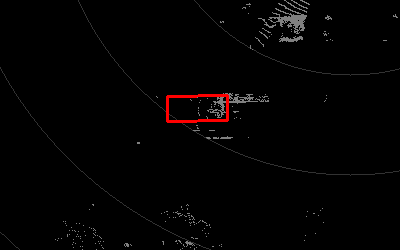
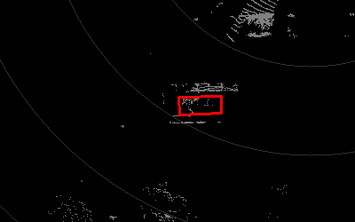
Figure 5. Example of an unlikely track. Predictions are inconsistent within a track, suggesting that they are spurious.

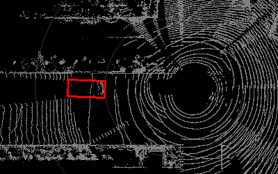
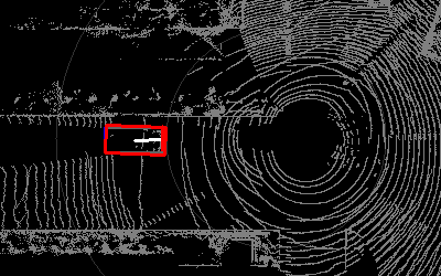
Figure 6. Example of missing human label within a track that Fixy can find. The left panel only contains an ML model prediction while the right contains both a human label and an ML model prediction.

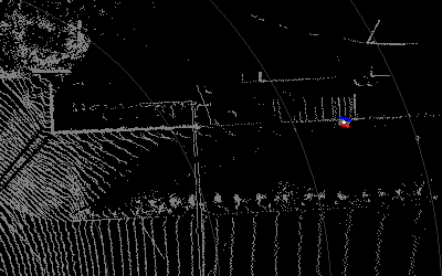
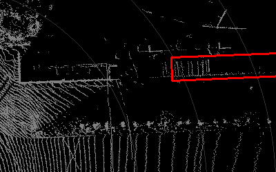
Figure 7. Example of a low probability bundle that would have a low rank. The box of the person and truck highly overlap, but are strongly inconsistent in box volume.

Finding missing labels within tracks. We are interested in finding errors in labels proposed by humans that should belong to an existing track. For example, Figure 6 shows a car trailing the AV, where the first frame is missing the car box.

To find such errors, we use the 3D bounding box prediction model’s predictions. The association of observations into bundles is done as above. The AOF zeros out the probability of any bundle that contains a human proposal and any track that does not contain any human proposals. Thus, the remaining bundles only contain ML model predictions and are in tracks that contain at least one human proposal.

The remaining bundles are scored as usual, with the intuition that predicted boxes that produce high probability bundles are likely to be correct predictions. We show an example of a high probability bundle (Figure 6) compared to a low probability bundle (Figure 7).

Finding erroneous ML model predictions. In this application, we are interested in finding erroneous ML model predictions. As such, we assume there are no human proposals. We show an example of an erroneous track in Figure 9, where the truck is inconsistently predicted.

The AOF inverts the probability of each feature, with the goal of inverting the ranking of the tracks that are likely to be correct and the tracks that are likely to be incorrect.

8. Evaluation

We evaluated Fixy on whether it can find errors in ML pipelines. We show that Fixy can find errors in human-proposed labels that are difficult to specify with ad-hoc MAs and novel errors in ML model predictions that prior work in ad-hoc MAs and uncertainty sampling cannot find.

8.1. Experimental Setup

Datasets. We evaluated Fixy on two AV perception datasets: an internal dataset from our research organization and the publicly available Lyft Level 5 perception dataset (Kesten et al., 2019). The Lyft dataset has been used to develop models (Zhu et al., 2019) and host competitions (Shet, 2019). Both datasets consists of many scenes of LIDAR and camera data that were densely labeled with 3D bounding boxes by leading external vendors for human labels (“human-proposed labels”).

We executed Fixy on 46 scenes from the Lyft dataset (the entire validation set, i.e., not seen at training time) and 13 scenes from our internal dataset. Additionally, we asses the recall of Fixy on a scene from our internal dataset that we vetted carefully.

The class labels, sampling rate, and physical sensor layout differ between the two datasets, showing that Fixy can apply across dataset characteristics.

Observation sources. We used three sources of observations over the data: human-proposed labels, LIDAR ML model predictions (Lang et al., 2019; Zhu et al., 2019), and expert auditor labels. All sources predict 3D bounding boxes. We focus on the common classes of car, truck, pedestrian, and motorcycle.

Features. We used the features shown in Table 2. These features consist of features that were automatically learned from data (volume, velocity, count) in addition to features for selecting more egregious errors (distance, model only).

Baselines. We compared against manually designed ad-hoc MAs developed by Kang et al. (2020) and uncertainty sampling. The ad-hoc MAs were designed to find errors in similar settings to ours, across both human-proposed labels and ML model predictions. Uncertainty sampling is commonly used in active learning (Settles, 2009).

As we describe (Section 3), the users of Fixy are typically non-experts in coding and ML tools. As such, we focus on simple ad-hoc MAs (e.g., ones developed by Kang et al. (2020)) and low-code features in Fixy. Each feature required fewer than 6 lines of code to implement.

Furthermore, both datasets were vetted by leading vendors for human labels. Thus, we find errors that were not found in an external audit.

Runtime. Since Fixy is primarily designed to operate in batch on ingested data and shown to auditors, the latency per scene is not a critical metric. Fixy executes in under five seconds on a single CPU core for processing a 15 second scene of data. For context, auditing a scene of data takes orders of magnitude longer, so this latency can easily be hidden.

Name	Type	Description
Volume	Obs.	Class-conditional box volume
Distance	Obs.	Distance to AV
Model only	Bundle	Selects bundles with model predictions only
Velocity	Trans.	Class-conditional object velocity
Count	Track	Filters tracks with two or fewer obs.

Table 2. Description of features we used in this evaluation. Model only and count were manually specified features.

8.2. Fixy can Find Missing Tracks

We investigated whether Fixy could find errors in vendor-proposed labels. We searched for tracks that were entirely missed by human proposals, as these errors are the most egregious.

Experimental setup. To find tracks entirely missed by human labelers, we associated LIDAR observations and human observations by box overlap within the same frame and associated observations within a track by box overlap across time. We further deployed the features described above. For the ad-hoc MA baseline, we used the “consistency” assertion as described by Kang et al. (2020). For comparison purposes, we ordered the ML model predictions randomly and by model confidence.

Method	Dataset	Precision at top 10	Precision at top 5	Precision at top 1
Fixy	Lyft	69%	70%	67%
Ad-hoc MA (rand)	Lyft	32%	30%	24%
Ad-hoc MA (conf)	Lyft	39%	40%	39%
Fixy	Internal	76%	100%	100%
Ad-hoc MA (rand)	Internal	49%	64%	66%
Ad-hoc MA (conf)	Internal	71%	86%	66%

Table 3. Precision at top 10 of Fixy and ad-hoc MA baselines for finding tracks missed by humans. Fixy used features and ad-hoc MAs used the consistency assertion described by Kang et al. (2020). Fixy outperforms baselines by up to 2$\times$.

We manually checked the top 10 potential errors as proposed by Fixy and ad-hoc model assertions (in some cases, fewer than 10 potential errors were flagged; we use the maximum number in these cases). We measured the precision among these potential errors, where a higher precision indicates that there are more errors within the top 10 proposals. For the Lyft dataset, we measured the precision across every scene in the validation set (i.e., data that was not seen during model training) that we discovered errors. For our internal dataset, we focused on the scene that failed audit.

Results: recall. To assess the recall of Fixy, we exhaustively audited a 15 second scene from our internal dataset. It contained 24 missing tracks. In this scene, Fixy achieved a recall of 75%, finding 18 of the missing tracks in the top 10 ranked errors per-class. We believe this result is reflective of the larger dataset.

We further manually searched for errors in the Lyft dataset and found errors in 32 of the 46 scenes. Unfortunately, due to the sheer number of errors in the Lyft dataset, we were unable to perform recall experiments on the level of boxes. However, LOA found errors in 100% of the scenes with errors in the top 10 ranked errors.

Results: precision. Fixy outperforms on finding errors on precision in both datasets (Table 3) by aggregating information across observations in tracks, which is difficult to do with ad-hoc MAs.

(a) Example of a missing car in motion.

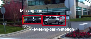
(b) Example of a missing car in motion.

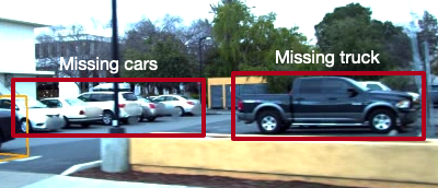
(c) Example of missing cars.

Figure 8. Examples of labeling errors in the Lyft dataset. The missing objects in these examples can be within 20 meters the autonomous vehicle and several are in motion: vehicles in motion are the most important to detect.

We show three examples of errors Fixy found in the Lyft dataset in Figure 8. Many of these errors are close to the AV and are clearly visible. These errors are problematic because they can confuse ML models and could potentially cause downstream issues.

Discussion. To further contextualize our results, we note that Fixy uncovered an error that was missed by an internal audit. Specifically, the motorcycle track described in Section 7 (Figure 4) was not found in our initial internal audit. Given the short time period the motorcycle was visible, it can be difficult to find for both crowd workers and auditors. Nonetheless, it is critical to be accurately labeled for two key reasons. First, clean training data is critical for liability purposes should an accident occur. Second, the motorcycle is close to the autonomous vehicle, which is especially problematic for downstream planning.

We note that our internal model does better than the public model. This is primarily because the Lyft dataset is very noisy: our internal model was trained on already audited data, which is of higher quality and results in more calibrated model predictions. These results highlight the need for high quality data: noisy data results in lower performing models.

Furthermore, the open-sourced Lyft perception dataset has a number of vehicles that were not labeled. We plan to open source the errors we have found to aid in the development of consistent labeling for the Lyft dataset.

8.3. Fixy can Find Missing Observations

We additionally searched for missing observations in human-proposed tracks as a case study. To find missing human-proposed labels within tracks, we applied the following AOF. We set the probability of an observation in a bundle with a human proposal to 0. We set the probability of any track without a human proposal to 0. For Fixy, we then ranked the bundles by likelihood. For the ad-hoc MA baseline, we random ordered bundles.

Within the datasets, we were only able to find a single example of such a missing observation. For this example, Fixy ranked the missing observation at the top. We show the missing observation in Figure 6 and examples of low probability missing observations in Figure 7. The feature distributions correctly identify consistent predictions within tracks and correctly downweights inconsistent predictions.

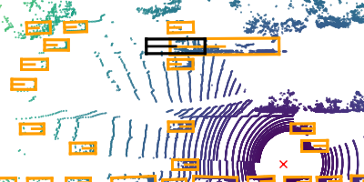
(a) $t=0$

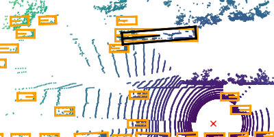
(b) $t=1$

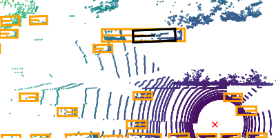
(c) $t=2$

Figure 9. Example of a model error (in black) in the Lyft dataset not found by ad-hoc model assertions. We show ground-truth boxes from human labels in orange for reference. The erroneous prediction overlaps across frames, but is not consistent. Fixy can find such errors as they produce unlikely values under learned feature distributions.

8.4. Fixy can Find Novel ML Prediction Errors

We further investigated whether or not Fixy can find errors in LIDAR model predictions. For this use-case, we did not assume access to human-proposed labels.

Experimental setup. Unlike for finding errors in human-proposed labels, ad-hoc MAs can achieve high precision when searching for errors in ML model predictions. As such, we deployed three ad-hoc MAs as used in Kang et al. (2020) (appear, flicker, and multibox). Briefly, the appear assertion asserts that an observation should have observations in nearby timestamps, the flicker assertion asserts than an observation should not appear and disappear rapidly, and the multibox assertion asserts that 3 boxes should not overlap. These assertions can be reproduced in Fixy with hand-tuned features.

In addition to ad-hoc MAs, we additionally compared to uncertainty sampling, in which we sampled predictions around a confidence threshold.

We then deployed Fixy to find errors in ML model prediction after excluding the errors found by these ad-hoc MAs. We searched for both localization and classification errors. For Fixy, we deployed the same features as above with the exception of distance and model only. We additionally deployed a track feature over the total number of observations. We measure the precision of the top 10 potential errors over 5 scenes in the Lyft dataset.

Results and discussion. Across these scenes, Fixy achieves a precision at 10 of 82% while uncertainty sampling achieved a precision of 42%. We note that errors we found with Fixy were not found by ad-hoc MAs. Many of these errors have tracks without missing time stamps (so will not trigger the flicker assertion) and are longer than two observations (so will not trigger the appear assertion). We show an example of such a track in Figure 9, in which the predictions overlap across frames, but in an unlikely way.

Furthermore, in contrast to uncertainty sampling, Fixy uncovers errors with high model confidence. Fixy discovered errors in ML model predictions with confidences as high as 95%, which uncertainty sampling would miss.

9. Related Work

Data cleaning. Data quality is of paramount concern, especially in ML pipelines. Work in the data systems community has focused on cleaning tabular data (Chu et al., 2016; Rahm and Do, 2000). This work focuses largely on detecting errors via constraints (Bertossi, 2006; Beskales et al., 2010; Bohannon et al., 2005) and more recently machine learning (Krishnan et al., 2016; Rekatsinas et al., 2017; Heidari et al., 2019). Unfortunately, these techniques do not directly apply to the labels in many ML pipelines, thus necessitating the need for new abstractions and systems for ML data.

Enriching data and weak supervision. Other work in the data systems community aims to clean or enrich data, often with the goal of training ML models. For example, HoloClean automatically aggregates noisy cleaning rules in a statistical fashion (Rekatsinas et al., 2017; Heidari et al., 2019). In this work, we focus on high quality training data in mission-critical settings as opposed to noisy cleaning rules.

Other work uses weak labels or organizational resources to train models with little labeled data. For example, users can specify noisy labeling functions that are aggregated to train models (Ratner et al., 2020). Other work uses organizational resources, e.g., embeddings and knowledge bases, to adapt models to new modalities (Suri et al., 2020). In mission-critical pipelines, these methods still need to be validated with a high-quality dataset, so require labels (Ratner et al., 2020). We leverage different organizational resources (existing labels and models) to find errors in labels, as opposed to training new models with fewer labels.

ML testing. According to a recent survey (Zhang et al., 2020), existing work in ML testing focuses on pipelines where schemas have meaningful information, such as categorical or numeric data (Hynes et al., 2017; Polyzotis et al., 2019, 2017). While important for deployments with schemas, they do not apply to the settings we consider. Other work considers statistical measures of accuracy (Amershi et al., 2019), fuzzing for numeric errors (Odena et al., 2019), worst case perturbations (Xiang et al., 2018), data linting (Hynes et al., 2017), and other techniques (Pham et al., 2019). These approaches are complementary to Fixy.

In this work, we primarily focus on finding errors in complex perception training data and model errors. To our knowledge, model assertions are closest line of work; see Section 2 for an extended discussion of MAs (Kang et al., 2020). Briefly, users must manually specify MAs and severity scores, which can be challenging in practice and miss important classes of errors.

Factor graphs. The closest analog of LOA in the Bayesian setting are factor graphs (Dellaert et al., 2017; Kschischang et al., 2001) that are widely used in robot perception. Factor graphs are a probabilistic tool to encode and factorize the joint distribution of random variables as a product of locally, conditionally independent functions. Modern mapping (Mur-Artal et al., 2015), tracking (Pöschmann et al., 2020), and localization (Dellaert et al., 2017) in robot perception use factor graphs to incorporate spatiotemporal, and multi-modal measurements into a probabilistic framework for Bayesian interpretation. We formulate a similar graphical framework to jointly reason over domain-specific feature distributions and application objective functions, composing together to form MA graphs. However, unlike robot perception applications that incorporate raw sensor measurements as individual factors, we incorporate both model predictions and object priors as factors in Fixy in order to acausally reason over the individual model prediction measurements.

10. Discussion and Future Work

We believe that Fixy is an exciting first step towards data management for complex, unstructured ML data. However, while effective at its particular task, many questions remain.

For example, Fixy was tailored for autonomous vehicle sensor data, but it may also be applicable to other domains with temporal aspects, such as audio or time series data. We view ML data management in a variety of domains, both for unstructured and structured data, to be an exciting area of future research.

Fixy also assumes independence between features and that features are not misspecified. While these assumptions produce reasonable results, more sophisticated graphical models and learning may help in ML data management.

11. Conclusion

To address the problem of finding errors in labels and ML models, we propose Learned Observation Assertions (LOA) and implement Fixy. LOA allows users to specify data-driven feature distributions to indicate which data points are potentially erroneous. Our prototype implementation of LOA, Fixy, leverages existing organizational resources (trained ML models and existing labeled data) to find labeling errors. We show that Fixy can find errors in human labels up to 2$\times$ more effectively than prior research work.

References

- (1)
- Amershi et al. (2019) Saleema Amershi, Andrew Begel, Christian Bird, Robert DeLine, Harald Gall, Ece Kamar, Nachiappan Nagappan, Besmira Nushi, and Thomas Zimmermann. 2019. Software engineering for machine learning: A case study. In 2019 IEEE/ACM 41st International Conference on Software Engineering: Software Engineering in Practice (ICSE-SEIP). IEEE, 291–300.
- Baylor et al. (2017) Denis Baylor, Eric Breck, Heng-Tze Cheng, Noah Fiedel, Chuan Yu Foo, Zakaria Haque, Salem Haykal, Mustafa Ispir, Vihan Jain, Levent Koc, et al. 2017. Tfx: A tensorflow-based production-scale machine learning platform. In Proceedings of the 23rd ACM SIGKDD International Conference on Knowledge Discovery and Data Mining. 1387–1395.
- Bertossi (2006) Leopoldo Bertossi. 2006. Consistent query answering in databases. ACM Sigmod Record 35, 2 (2006), 68–76.
- Beskales et al. (2010) George Beskales, Ihab F Ilyas, and Lukasz Golab. 2010. Sampling the repairs of functional dependency violations under hard constraints. Proceedings of the VLDB Endowment 3, 1-2 (2010), 197–207.
- Bohannon et al. (2005) Philip Bohannon, Wenfei Fan, Michael Flaster, and Rajeev Rastogi. 2005. A cost-based model and effective heuristic for repairing constraints by value modification. In Proceedings of the 2005 ACM SIGMOD international conference on Management of data. 143–154.
- Cheng (2019) Chiao-Lun Cheng. 2019. Training Data - Quantity is no Panacea. (2019). https://scale.com/blog/training-data-quantity-is-no-panacea
- Chu et al. (2016) Xu Chu, Ihab F Ilyas, Sanjay Krishnan, and Jiannan Wang. 2016. Data cleaning: Overview and emerging challenges. In Proceedings of the 2016 international conference on management of data. 2201–2206.
- Dellaert et al. (2017) Frank Dellaert, Michael Kaess, et al. 2017. Factor graphs for robot perception. Foundations and Trends® in Robotics 6, 1-2 (2017), 1–139.
- Heidari et al. (2019) Alireza Heidari, Joshua McGrath, Ihab F Ilyas, and Theodoros Rekatsinas. 2019. Holodetect: Few-shot learning for error detection. In Proceedings of the 2019 International Conference on Management of Data. 829–846.
- Hynes et al. (2017) Nick Hynes, D Sculley, and Michael Terry. 2017. The data linter: Lightweight, automated sanity checking for ml data sets. In NIPS MLSys Workshop.
- Kang et al. (2020) Daniel Kang, Deepti Raghavan, Peter Bailis, and Matei Zaharia. 2020. Model Assertions for Monitoring and Improving ML Model. MLSys (2020).
- Kaparthy (2018) Andrej Kaparthy. 2018. Building the Software 2.0 Stack. (2018).
- Kesten et al. (2019) R. Kesten, M. Usman, J. Houston, T. Pandya, K. Nadhamuni, A. Ferreira, M. Yuan, B. Low, A. Jain, P. Ondruska, S. Omari, S. Shah, A. Kulkarni, A. Kazakova, C. Tao, L. Platinsky, W. Jiang, and V. Shet. 2019. Lyft Level 5 Perception Dataset 2020. https://level5.lyft.com/dataset/.
- Krishnan et al. (2016) Sanjay Krishnan, Jiannan Wang, Eugene Wu, Michael J Franklin, and Ken Goldberg. 2016. Activeclean: Interactive data cleaning while learning convex loss models. arXiv preprint arXiv:1601.03797 (2016).
- Kschischang et al. (2001) Frank R Kschischang, Brendan J Frey, and H-A Loeliger. 2001. Factor graphs and the sum-product algorithm. IEEE Transactions on information theory 47, 2 (2001), 498–519.
- Lang et al. (2019) Alex H Lang, Sourabh Vora, Holger Caesar, Lubing Zhou, Jiong Yang, and Oscar Beijbom. 2019. Pointpillars: Fast encoders for object detection from point clouds. In Proceedings of the IEEE Conference on Computer Vision and Pattern Recognition. 12697–12705.
- Mur-Artal et al. (2015) Raul Mur-Artal, Jose Maria Martinez Montiel, and Juan D Tardos. 2015. ORB-SLAM: a versatile and accurate monocular SLAM system. IEEE transactions on robotics 31, 5 (2015), 1147–1163.
- Odena et al. (2019) Augustus Odena, Catherine Olsson, David Andersen, and Ian Goodfellow. 2019. Tensorfuzz: Debugging neural networks with coverage-guided fuzzing. In International Conference on Machine Learning. 4901–4911.
- Pham et al. (2019) Hung Viet Pham, Thibaud Lutellier, Weizhen Qi, and Lin Tan. 2019. CRADLE: cross-backend validation to detect and localize bugs in deep learning libraries. In 2019 IEEE/ACM 41st International Conference on Software Engineering (ICSE). IEEE, 1027–1038.
- Polyzotis et al. (2017) Neoklis Polyzotis, Sudip Roy, Steven Euijong Whang, and Martin Zinkevich. 2017. Data management challenges in production machine learning. In Proceedings of the 2017 ACM International Conference on Management of Data. 1723–1726.
- Polyzotis et al. (2019) Neoklis Polyzotis, Martin Zinkevich, Sudip Roy, Eric Breck, and Steven Whang. 2019. Data validation for machine learning. MLSys (2019).
- Pöschmann et al. (2020) Johannes Pöschmann, Tim Pfeifer, and Peter Protzel. 2020. Factor Graph based 3D Multi-Object Tracking in Point Clouds. arXiv preprint arXiv:2008.05309 (2020).
- Rahm and Do (2000) Erhard Rahm and Hong Hai Do. 2000. Data cleaning: Problems and current approaches. IEEE Data Eng. Bull. 23, 4 (2000), 3–13.
- Ratner et al. (2020) Alexander Ratner, Stephen H Bach, Henry Ehrenberg, Jason Fries, Sen Wu, and Christopher Ré. 2020. Snorkel: rapid training data creation with weak supervision. The VLDB Journal 29, 2 (2020), 709–730.
- Rekatsinas et al. (2017) Theodoros Rekatsinas, Xu Chu, Ihab F Ilyas, and Christopher Ré. 2017. Holoclean: Holistic data repairs with probabilistic inference. arXiv preprint arXiv:1702.00820 (2017).
- Settles (2009) Burr Settles. 2009. Active learning literature survey. Technical Report. University of Wisconsin-Madison Department of Computer Sciences.
- Shet (2019) Vinay Shet. 2019. Lyft Level 5 Self-Driving Perception Dataset Competition Now Open. https://medium.com/wovenplanetlevel5/lyft-level-5-self-driving-dataset-competition-now-open-97493e9f154a. (2019).
- Suri et al. (2020) Sahaana Suri, Raghuveer Chanda, Neslihan Bulut, Pradyumna Narayana, Yemao Zeng, Peter Bailis, Sugato Basu, Girija Narlikar, Christopher Ré, and Abishek Sethi. 2020. Leveraging organizational resources to adapt models to new data modalities. arXiv preprint arXiv:2008.09983 (2020).
- Wakabayashi (2018) Daisuke Wakabayashi. 2018. Self-Driving Uber Car Kills Pedestrian in Arizona, Where Robots Roam. https://www.nytimes.com/2018/03/19/technology/uber-driverless-fatality.html.
- Wandinger (2005) Ulla Wandinger. 2005. Introduction to lidar. In Lidar. Springer, 1–18.
- Xiang et al. (2018) Weiming Xiang, Patrick Musau, Ayana A Wild, Diego Manzanas Lopez, Nathaniel Hamilton, Xiaodong Yang, Joel Rosenfeld, and Taylor T Johnson. 2018. Verification for machine learning, autonomy, and neural networks survey. arXiv preprint arXiv:1810.01989 (2018).
- Zhang et al. (2020) Jie M Zhang, Mark Harman, Lei Ma, and Yang Liu. 2020. Machine learning testing: Survey, landscapes and horizons. IEEE Transactions on Software Engineering (2020).
- Zhu et al. (2019) Benjin Zhu, Zhengkai Jiang, Xiangxin Zhou, Zeming Li, and Gang Yu. 2019. Class-balanced Grouping and Sampling for Point Cloud 3D Object Detection. arXiv preprint arXiv:1908.09492 (2019).