Deep Optimal Transport for Domain Adaptation on SPD Manifolds

Abstract

In recent years, there has been significant interest in solving the domain adaptation (DA) problem on symmetric positive definite (SPD) manifolds within the machine learning community. This interest stems from the fact that complex neurophysiological data generated by medical equipment, such as electroencephalograms, magnetoencephalograms, and diffusion tensor imaging, often exhibit a shift in data distribution across different domains. These data representations, represented by signal covariance matrices, possess properties of symmetry and positive definiteness. However, directly applying previous experiences and solutions to the DA problem poses challenges due to the manipulation complexities of covariance matrices.To address this, our research introduces a category of deep learning-based transfer learning approaches called deep optimal transport. This category utilizes optimal transport theory and leverages the Log-Euclidean geometry for SPD manifolds. Additionally, we present a comprehensive categorization of existing geometric methods to tackle these problems effectively. This categorization provides practical solutions for specific DA problems, including handling discrepancies in marginal and conditional distributions between the source and target domains on the SPD manifold. To evaluate the effectiveness, we conduct experiments on three publicly available highly non-stationary cross-session brain-computer interface scenarios. Moreover, we provide visualization results on the SPD cone to offer further insights into the framework.

1 Introduction

I n cross-domain problems, the distribution of source data typically differs from that of target data, giving rise to what is commonly known as the domain adaptation (DA) problem in the machine learning community. Over the past decade, this issue has garnered significant attention [1, 2, 3]. For instance, in signal processing, it is common for a signal in the online testing set to differ from a realization of the same process that generates the calibration set, thereby exemplifying a typical DA problem.

In a DA problem, a domain $\mathcal{D}$ consists of a feature space $X$ and a marginal probability distribution $\mathbb{P}(X)$, denoted as $\mathcal{D}=\{X,\mathbb{P}(X)\}$. Meanwhile, a task $\mathcal{T}$ comprises a label space $Y$ and a predictive function $\mathbb{P}(Y|X)$, represented by $\mathcal{T}=\{Y,\mathbb{Q}(Y|X)\}$. The DA problem aims to build a classifier in the target domain $\mathcal{D}_{T}$ by leveraging the information obtained from the source domain $\mathcal{D}_{S}$, where $\mathcal{D}_{S}\neq\mathcal{D}_{T}$ and $\mathcal{T}_{S}\neq\mathcal{T}_{T}$. In particular, $\mathcal{D}_{S}\neq\mathcal{D}_{T}$ yields either $X_{S}\neq X_{T}$ or $\mathbb{P}_{S}(X_{S})\neq\mathbb{P}_{T}(X_{T})$, whereas $\mathcal{T}_{S}\neq\mathcal{T}_{T}$ results in either $Y_{S}\neq Y_{T}$ or $\mathbb{Q}_{S}(Y_{S}|X_{S})$ or $\mathbb{Q}_{T}(Y_{T}|X_{T})$. The DA problem can be broadly categorized into unsupervised and semi-supervised domain adaptation. The former assumes the absence of labels in the target domain, while the latter presupposes the availability of a limited number of labeled instances in the target domain, which serve as reference points for the adaptation process. For instance, the variability of electroencephalography (EEG) signals frequently results in untrustworthy and non-robust performance when transitioning from calibration to feedback phases, as the two sessions exhibit distinct distributions. This represents a typical domain adaptation problem [4]. To address this variability, Sugiyama [5] applied their covariate shift adaptation approach to EEG scenarios, assuming that the difference between domains is characterized by a change in the feature space while conditional distributions remain unchanged, that is, $\mathbb{P}_{S}(X_{S})\neq\mathbb{P}_{T}(X_{T})$ and $\mathbb{Q}_{S}(Y_{S}|X_{S})=\mathbb{Q}_{T}(Y_{T}|X_{T})$.

TABLE I: Evolutionary History of the OT-DA Framwork.  

	Cost function	Transformation	Underlying Space	Scenario
OT-DA[6, 7]	$c(x,\bar{x})=||x-\bar{x}||_{\ell_{2}}^{2}.$	Affine.	Euclidean.	$X_{S}\neq X_{T}$.
JDOT-DA[8, 9]	$c(x,\bar{x})=||x-\bar{x}||_{\ell_{2}}^{2}$.	Affine.	Euclidean.	$X_{S}\neq X_{T}$, $\mathbb{Q}_{S}(Y_{S}|X_{S})\neq\mathbb{Q}_{T}(Y_{T}|X_{T})$.
OT-DA on SPD manifolds[10]	$c(x,\bar{x})=||x-\bar{x}||_{\ell_{2}}^{2}$.	Bi-Map.	($\mathcal{S}_{++}$, $g^{AIRM}$).	$X_{S}\neq X_{T}$.
DOT (proposed)	$c(x,\bar{x})=d_{g^{LEM}}^{2}(x,\bar{x}).$	Neural Networks	($\mathcal{S}_{++}$, $g^{LEM}$).	$X_{S}=X_{T}$, $\mathbb{P}_{S}(X_{S})\neq\mathbb{P}_{T}(X_{T})$, and
		on SPD manifolds		$\mathbb{Q}_{S}(Y_{S}|X_{S})\neq\mathbb{Q}_{T}(Y_{T}|X_{T})$.

Although various existing methods have been proposed for the DA problem, Optimal Transport (OT) has emerged as a novel solution that can align the source and target domains more effectively. Courty introduced the concept of regularized optimal transport, enabling the classifier to learn from labeled source data and apply it to target data [6, 7]. The objective is to minimize the overall transportation cost between two distributions with an associated divergence known as the Wasserstein metric, thereby finding a push-forward transformation $\varphi:X_{S}\longmapsto X_{T}$ that satisfies $\mathbb{P}_{S}(X_{S})=\mathbb{P}_{T}(\varphi(X_{S}))$. We henceforth refer to their framework as the OT-DA framework. The strengths of the OT-DA framework lie in its simplified evaluation of empirical estimation of data distribution and its improved ability to leverage the underlying geometry of discrete samples [6]. However, the OT-DA framework, while broad, is relatively rudimentary, and can be further enhanced by deriving insights from specific engineering scenarios. For instance, in the EEG-based Brain-Computer Interfacing (BCI) system, engineers process EEG signals using its spatial covariance matrices [11, 12]. This leads to all classification tasks taking place on the space of spatial covariance matrices from a perspective of Symmetric Positive Definite (SPD) manifolds when endowed with a Riemannian metric [13, 14, 15]. Addressing this context on SPD manifolds, Yair [10] propose the utilization of squared $\ell_{2}$ distance as the cost function $c(x,\bar{x})=||x-\bar{x}||_{\ell_{2}}^{2}$ for the OT problem, subsequently deriving a closed-form solution by means of Brenier’s polar factorization[16].

Despite being the pioneering OT-DA framework for SPD matrices, Yair’s work presents certain theoretical and practical shortcomings. From a theoretical standpoint, their chosen cost function, grounded in Euclidean distance, compromises the geometric coherence of the framework. From a practical standpoint, their methodology overlooks the modeling of disparities within conditional distributions. Furthermore, the unique difficulties intrinsic to the problem, including the scarcity of labeled EEG signals during the feedback phase and the divergence of spatial covariance matrices produced from distinct frequency bands from any standard probability distribution, pose considerable difficulties for modeling. These challenges necessitate the development of a more adaptable OT-DA framework to adequately address problems on SPD manifolds.

To circumvent these challenges, we consider a more applicable scenario where $X_{S}=X_{T}$, $Y_{S}=Y_{T}$, $\mathbb{P}_{S}(X_{S})\neq\mathbb{P}_{T}(X_{T})$, and $\mathbb{Q}_{S}(Y_{S}|X_{S})\neq\mathbb{Q}_{T}(Y_{T}|X_{T})$. This situation is typically addressed via joint distribution adaptation, which concurrently adapts both marginal and conditional distributions across domains. This holds even for implicit probability distributions, all the while circumventing reliance on labeled information for the target domain [17]. To facilitate the modeling of $X_{S}=X_{T}$, we employ the Log-Euclidean metric $g^{LEM}$ [18] as the Riemannian metric for the space of SPD matrices. We denote this kind of SPD manifolds as ($\mathcal{S}_{++}$, $g^{LEM}$). Under this metric, the parallel transport corresponds to the identity map, which implies that the feature space (i.e., tangent vectors on the tangent space of SPD manifolds) remains consistent. We also introduce a deep learning-based category for the joint distribution adaptation problem on ($\mathcal{S}_{++}$, $g^{LEM}$), endowed with a squared cost function $c(x,\bar{x})=d_{g^{LEM}}^{2}(x,\bar{x})$. This is referred to as the category of Deep Optimal Transport (DOT).

The category of DOT can be considered as an umbrella term encompassing all deep transfer learning approaches on ($\mathcal{S}{++}$, $g^{LEM}$) that employ optimal transport. This is based on the assumption that the transfer of information between domains can be estimated through optimal transport. The objective of DOT is to find a transformation on SPD manifolds, denoted as $\varphi:X_{S},X_{T}\longmapsto Z\subset\mathcal{S}_{++}$, which satisfies the conditions $\mathbb{P}_{S}(\varphi(X_{S}))\neq\mathbb{P}_{T}(\varphi(X_{T}))$ and $\mathbb{Q}_{S}(Y_{S}|\varphi(X_{S}))\neq\mathbb{Q}_{T}(Y_{T}|\varphi(X_{T}))$. These conditions indicate that all methods within the DOT category can be viewed as a type of subspace alignment method in the context of transfer learning [19]. Based on our definition of this category, one existing method within the DOT category is called Deep Joint Distribution Optimal Transport (DeepJDOT) [9]. DeepJDOT extends the Joint Distribution Optimal Transport (JDOT) framework [8] by concurrently optimizing the optimal coupling and prediction functions for two distributions defined in a shared space, using a deep learning-based architecture. Once the associated divergence is represented by the Riemannian distance on SPD manifolds, the natural extension of DeepJDOT would be to ($\mathcal{S}_{++}$, $g^{LEM}$). In this study, we will propose additional methods belonging to the DOT category that address other joint distribution adaptation problems induced by subtasks in BCI research.

To evaluate the effectiveness of DOT, we focus on a key problem in the field of BCIs, namely cross-session motor imagery (MI) EEG classification. This problem is typically challenging and inadequately addressed, primarily due to the extensive patterns of synchronized neuronal activity that perpetually shift over time, resulting in significant variability of brain signals captured by EEG devices across sessions. We calibrate the model in one session and evaluate it in another. The testing scenario includes both unsupervised and semi-supervised domain adaptation problems.

The remainder of this paper is organized as follows: Section 2 delves into the research history of MI-EEG classifiers, the mathematical formulations for both continuous and discrete OT problems, and the Joint Distribution Optimal Transport problem. Section 3 presents the OT-DA framework on SPD manifolds, and proposes the category of DOT. In Section 4, we will apply the proposed DOT on the MI-EEG classifier with three assumptions, introduce the construction of three MI-EEG experimental datasets and testing scenarios, as well as categorize all geometric methods used for domain adaptation in MI-EEG tasks. Section 5 will exhibit results from synthetic and real-world datasets. In the discussion section, we will further discuss some of the topics touched upon throughout the paper. A comparison of Country’s, Yair’s, and the proposed category is encapsulated in Table I.

2 PRELIMINARY

Generalizing an OT-DA framework to SPD manifolds poses significant challenges. The primary obstacle is to devise an effective computational strategy that addresses the inherent computational complexities of SPD manifolds.

Fortunately, extensive research has been conducted on computational methodologies for engineering applications on SPD manifolds, involving one or multiple categories of Riemannian metrics. During the early stages of feature engineering, Xavier explored various classes of Riemannian metrics on SPD manifolds for a wide range of applications. This exploration led to the introduction of numerous statistical computational methodologies to tackle issues related to SPD manifolds, drawing inspiration from manifold-valued images, such as Diffusion Tensor Imaging [20, 21, 22, 23, 24]. Moreover, Barachant investigated spatial covariance matrices of EEG signals on SPD manifolds using affine invariant Riemannian metric. The study resulted in the development of several effective MI-EEG classifiers, influenced by Xavier’s approaches, which impact various BCI applications [13, 14, 15, 25, 26].

Following the emergence of the deep learning era, Huang proposed a series of innovative Riemannian-based network architectures as computational methodologies for learning on SPD manifolds, encompassing one or multiple classes of Riemannian metrics [27, 28, 29]. By employing Huang’s network architectures on SPD manifolds, Ju established geometric deep learning paradigms to leverage attributes within the time-space-frequency domain embedded within spatial covariance matrices on SPD manifolds for MI-EEG classification, ultimately enhancing performance [30, 31, 32, 33].

2.1 Log-Euclidean Geometry

A matrix $S\in\mathbb{R}^{n\times n}$ is said to be SPD if it is symmetric and all its eigenvalues are positive, i.e.,

$$S=S^{T},\quad\text{and}\quad x^{T}\cdot S\cdot x>0\quad\forall x\in\mathbb{R}^{n}\setminus\{{\mathbf{0}}\}.$$

The Log-Euclidean Metric $g^{LEM}$, which gives a vector space structure to the space of SPD matrices while possessing numerous exceptional properties, including invariance under inversion, logarithmic multiplication, orthogonal transformations, and scaling. It forms a vector space, rendering it flat and also a Cartan-Hadamard manifold [18, 21]. Formally, a commutative Lie group structure is endowed on $\mathcal{S}_{++}$ where the logarithmic multiplication $\odot$ and the logarithmic scalar multiplication $\otimes$ are defined as follows: for any $S,S_{1}$, and $S_{2}\in\mathcal{S}_{++}$,

$$S_{1}\odot S_{2} :=\exp{\big{(}\log(S_{1})+\log(S_{2})\big{)}};$$

$$\lambda\otimes S :=\exp{\big{(}\lambda\cdot\log(S)\big{)}}=S^{\lambda},$$

where $\exp$ and $\log$ are matrix exponential and logarithm respectively. In this work, we denote SPD manifolds $\mathcal{S}_{++}$ endowed with $g^{LEM}$ as ($\mathcal{S}_{++}$, $g^{LEM}$). The Log-Euclidean distance between any two matrices $S_{1}$ and $S_{2}$ on ($\mathcal{S}_{++}$, $g^{LEM}$) can be defined as follows:

$$d_{g^{LEM}}(S_{1},S_{2})=||\log{(S_{1})}-\log{(S_{2})}||_{\mathcal{F}}.$$ (1)

The Log-Euclidean Fr$\acute{e}$chet mean $\overline{w}(\mathcal{B})$ of a batch $\mathcal{B}$ of SPD matrices $\{S_{i}\}_{i=1}^{|\mathcal{B}|}\in(\mathcal{S}_{++},g^{LEM})$ is defined as follows:

$$\overline{w}(\mathcal{B}):=\exp{\bigg{(}\frac{1}{|\mathcal{B}|}\cdot\sum_{i}\log{(S_{i})}\bigg{)}}.$$ (2)

2.2 Monge-Kantorovich Formulation for Optimal Transportation

The optimal transportat problem, also referred to as the Monge-Kantorovich problem, is a mathematical framework that deals with the efficient and optimal movement of a distribution of mass from one configuration to another [34, 35]. This is achieved by minimizing a specified cost function, as first formalized by Monge [36]. Formally, a separable, completely metrizable topological space is called Polish space. On two Polish spaces $X$ and $\bar{X}$, given a Borel map $T:X\longmapsto\bar{X}$, $T_{\#}$ pushes forward $\mu\in\mathbb{P}(X)$ through $T$ to $T_{\#}\,\mu\in\mathbb{P}(\bar{X})$, i.e., $T_{\#}\,\mu(E):=\mu(T^{-1}(E))$, for any borel $E\subset\bar{X}$. The Monge formulation seeks to find the most efficient measure-preserving mapping $T$ between two distributions, as determined by a designated cost function as follows:

$$\min_{T\in S(\mu,\nu)}\int_{X}c(x,T(x))\,d\mu(x),$$

where $S(\mu,\nu)$ is a set of transports that pushes $\mu$ forward to $\nu$, and cost function $c:X\times\bar{X}\longmapsto\mathbb{R}_{\geq 0}$ is a given cost function. The Monge-Kantorovich formulation of the optimal transportation problem was further proposed by Kantorovich [37]. The revised problem can be stated as follows:

$$\min_{\gamma\in\prod(\mu,\nu)}\int_{X\times\bar{X}}c(x,\bar{x})\,d\gamma(x,\bar{x}),$$

where $\pi^{X}$ and $\pi^{\bar{X}}$ are the natural projections from $X\times\bar{X}$ onto $X$ and $\bar{X}$ respectively, and transportation plan $\gamma\in\prod(\mu,\nu):=\{\gamma\in\mathbb{P}(X\times\bar{X})\big{|}\pi^{X}_{\#}\cdot\gamma=\mu,\text{ and }\pi^{\bar{X}}_{\#}\cdot\gamma=\nu\}$.

2.3 Discrete Monge-Kantorovich Problem

Given a measurable space $X$ and $\bar{X}$, an empirical distribution of the measure $\mu\in X$ and $\nu\in\bar{X}$ are written as $\mu:=\sum_{i\in I}p_{i}\cdot\delta_{x_{i}}$ and $\nu:=\sum_{j\in J}q_{i}\cdot\delta_{\bar{x}_{i}}$, where discrete random varaiable $X$ takes values $\{x_{i}\}_{i\in I}\in X$, countable index set $I$ is with weights $\sum_{i\in I}p_{i}=1$. $\bar{X}$ takes values $\{\bar{x}_{j}\}_{j\in J}\in\bar{X}$, countable index set $J$ is with weights $\sum_{j\in J}q_{j}=1$. Dirac measure $\delta_{s}$ denotes a unite point mass at the point $s\in X\text{ or }\bar{X}$. The discrete Monge-Kantorovich problem in the OT theory is given as follows:

$$~{}\min_{\gamma\in\prod(\mu,\nu)}\big{\langle}\gamma,c(x,\bar{x})\big{\rangle}_{\mathcal{F}},$$ (3)

where transportation plan $\gamma\in\prod(\mu,\nu):=\{\gamma\in\mathbb{R}_{\geq 0}^{|X|\times|\bar{X}|}\big{|}\gamma\cdot\mathbbm{1}_{|X|}=\mu,\text{ and }\gamma^{\top}\cdot\mathbbm{1}_{|\bar{X}|}=\nu\}$, and $\mathbbm{1}_{d}$ is a $d-$dimensional all-one vector. The Frobenius inner product and Frobenius norm on $m\times n$ matrices $A$ and $B$ are defined as $\langle\,A,B\,\rangle_{\mathcal{F}}:=\operatorname{Tr}{(A^{\top}\cdot B)}$ and $||\,A\,||_{\mathcal{F}}^{2}:=\langle\,A,A\,\rangle_{\mathcal{F}}$ respectively.

2.4 (Deep) Joint Distribution Optimal Transport

Based on the assumption that the transfer between source and target domains can be estimated using optimal transport, Joint Distribution Optimal Transport (JDOT) [8] extends the OT-DA framework by jointly optimizing the optimal coupling and the prediction function $f$ for two distributions, i.e.,

$$\min_{\gamma\in\prod(\mu,\nu)}\big{\langle}\gamma,c^{\prime}(x,y;\bar{x},f(\bar{x}))\big{\rangle}_{\mathcal{F}},$$

where $y$ is the label set for samples $x$, $f$ is the prediction function, and the joint cost function is defined as follows,

$$~{}c^{\prime}(x,y;\bar{x},f(\bar{x}))=\alpha_{1}\cdot d_{\ell^{2}}(x,\bar{x})+\alpha_{2}\cdot\mathcal{L}(y,f(\bar{x})),$$ (4)

where $\alpha_{1},\alpha_{2}\geq 0$ and $\mathcal{L}$ is the classification loss, i.e., the cross-entropy loss. The deep learning-based extension of this work called DeepJDOT was proposed in [9]. DeepJDOT provides a joint objective function as follows,

$$\mathcal{L}=\mathcal{L}(y,f(g(x)))+\big{\langle}\gamma,c^{\prime}\big{(}g(x),y;g(\bar{x}),f(g(\bar{x})\big{)}\big{\rangle}_{\mathcal{F}},$$

where $g(x)$ is the nerual networks-based function that maps the raw data into feature space. In this work, it also presents a novel alternative update method, initially employing OT to solve for the transportation plan $\gamma$, and subsequently updating neural network parameters through regular stochastic gradient descent.

3 Methodology

This section will formalize the DA problem on ($\mathcal{S}_{++}$, $g^{LEM}$) in the OT framework. We call the new framework as the OT-DA framework on ($\mathcal{S}_{++}$, $g^{LEM}$).

3.1 OT-DA Framework on SPD Manifolds

In this section, we aim to establish the foundational principle for computing the optimal transport on ($\mathcal{S}_{++}$, $g^{LEM}$). To commence, we first articulate the representation of the gradient of any squared distance function on general Riemannian manifolds.

Lemma 1.

Let $(\mathcal{M},g)$ be a connected, compact, and $C^{3}-$smooth Riemannian manifold without a boundary. Consider a compact subset $\mathcal{U}\subset\mathcal{M}$ and a fixed point $q\in\mathcal{U}$. Let $f(p)=\frac{1}{2}\cdot d_{g}^{2}(p,q)$ denote the squared distance function. Then, for $p$ not on the boundary of $\mathcal{M}$, the gradient of $f(p)$ is given by $\nabla f(p)=-\log_{p}(q)$.

Proof.

Without loss of generality, consider a point $p\in\mathcal{M}^{\circ}$. There exists an open neighborhood $\mathcal{N}$ of $p$ and $\epsilon>0$ such that the exponential map $\exp_{p}$ maps the ball $\mathcal{B}(0,\epsilon)\subset T_{p}\mathcal{M}$ diffeomorphically onto $\mathcal{N}$ [49, Corollary 5.5.2.]. Let $c(s)$ be a geodesic on $\mathcal{N}$, parameterized with constant speed, with $c(0):=q\in\mathcal{N}$ and $c(1):=p$ with $\dot{c}(0)=\log_{q}(p)$. By reversing the direction of the geodesic $c(1-s)$, we have $\dot{c}(1)=-\log_{p}(q)$. We proceed by linearizing the exponential maps around $0\in T_{p}\mathcal{M}$ and $\dot{c}(0)\in T_{q}\mathcal{M}$ and derive the derivative of a function $f$ as follows:

$$f\big{(}\exp_{p}(v)\big{)}$$

$$=\, \frac{1}{2}\cdot d_{g}^{2}\big{(}\exp_{p}(v),q\big{)}$$

$$=\, \frac{1}{2}\cdot\big{|}\log_{q}\big{(}\exp_{p}(v)\big{)}\big{|}_{q}^{2}$$

$$=\, \frac{1}{2}\cdot\big{|}\dot{c}(0)+(D\log_{q})_{\dot{c}(0)}\big{(}(D\exp_{p})_{0}v\big{)}+o(|v|_{p})\big{|}_{q}^{2}$$

$$=\, \frac{1}{2}\cdot\big{|}\dot{c}(0)\big{|}_{q}^{2}+g_{q}(\dot{c}(0),(D\log_{q})_{\dot{c}(0)}v)+o(|v|_{p})$$

$$=\, \frac{1}{2}\cdot d_{g}^{2}(p,q)+g_{p}(\dot{c}(1),v)+o(|v|_{p}),$$

where the differential $(D\exp_{p})_{q}(\cdot):T_{q}(T_{p}\mathcal{M})\longmapsto(T_{p}\mathcal{M})$ is the differential of the exponential map at $q$ with respect to $p$. The fourth equality follows from $(D\exp_{p})_{0}=I$ on $T_{p}\mathcal{M}$, and the fifth equality follows from Gauss’ lemma [50, Section 3.3.5.]. Hence, by the definition of the gradient on Riemannian manifolds, we have $df(p)(v)=g_{p}\big{(}\nabla f(x),v\big{)}$, which implies that $\nabla f(p)=\dot{c}(1)=-\log_{p}(q)$. ∎

We say a function $\psi:\mathcal{M}\longmapsto\mathbb{R}\cup\{-\infty\}$ is c-concave if it is not identically $-\infty$ and there exists $\varphi:\mathcal{M}\longmapsto\mathbb{R}\cup\{\pm\infty\}$ such that

$$\psi(p)=\inf_{q\in\mathcal{M}}\big{\{}c(p,q)+\varphi(q)\big{\}},$$

where $c(p,q)$ is a nonnegative cost function that measures the cost of transporting mass from $q$ to $p\in\mathcal{M}$. Brenier’s polar factorization on general Riemannian manifolds is given as follows:

Lemma 2 (Brenier’s Polar Factorization [38]).

Given any compactly supported measures $\mu,\nu\in\mathbb{P}(\mathcal{M})$. If $\mu$ is absolutely continuous with respect to Riemannian volume, there exists a unique optimal transport map $T\in S(\mu,\nu)$ as follows,

$$T(x)=\exp_{p}\big{(}-\nabla\psi(p)\big{)},$$

where $\psi:\mathcal{M}\longmapsto\mathbb{R}\cup\{\pm\infty\}$ is a c-concave function with respect to the cost function $c(p,q)=\frac{1}{2}\cdot d_{g}^{2}(p,q)$, and $\exp_{p}(\cdot)$ is the exponential map at $p$ on $(\mathcal{M},g)$.

On the SPD manifold ($\mathcal{S}_{++}$, $g^{LEM}$), let’s consider source measure $\mu$ and target measure $\nu\in\mathbb{P}(\mathcal{S}_{++})$ that are accessible only through finite samples $\{S_{i}\}_{i=1}^{N}\sim\mu$ and $\{\bar{S}_{j}\}_{j=1}^{M}\sim\nu$. Each individual sample contributes to their respective empirical distribution with weights $\frac{1}{N}$ and $\frac{1}{M}$. We assume there exists a linear transformation on ($\mathcal{S}_{++}$, $g^{LEM}$) between two discrete feature space distributions of the source and target domains that can be estimated with the discrete Monge-Kantorovich problem 3, i.e., there exists

$$~{}\gamma^{\dagger}:=\arg\min_{\gamma\in\prod(\mu,\nu)}\big{\langle}\gamma,d_{g^{LEM}}^{2}(S,\bar{S})\big{\rangle}_{\mathcal{F}},$$ (5)

where $\prod(\mu,\nu):=\{\gamma\in\mathbb{R}_{\geq 0}^{N\times M}\big{|}\gamma\cdot\mathbbm{1}_{N}=\frac{1}{N},\text{ and }\gamma^{\top}\cdot\mathbbm{1}_{M}=\frac{1}{M}\}$. The pseudocode for the computation of the transport plan is presented in Algorithm 1.

Input  : Source samples $\{S_{i}\}_{i=1}^{N}\sim\mu$, target samples $\{\bar{S}_{j}\}_{j=1}^{M}\sim\nu$.

Output: Transport plan $\gamma$, and new coordinates for target samples $\{\bar{S}^{\dagger}_{j}\}_{j=1}^{M}$.

/* 1. Compute ground metric matrix for OT */

          $D(i,j)\leftarrow d_{g^{LEM}}(S_{i},\bar{S}_{j})$.

/* 2. Compute transport plan $\gamma$ using the earth movers distance-based OT algorithm. */

          $\gamma^{\dagger}\leftarrow OT^{EMD}(N,M,D(i,j))$.

/* 3. Compute new coordinates using transport plan on ($\mathcal{S}_{++}$, $g^{LEM}$). */

          $\{\bar{S}^{\dagger}_{j}\}_{j=1}^{M}\leftarrow\exp{\big{(}\gamma^{\dagger}[j,:]\cdot\{\log(S_{i})\}_{i=1}^{N}\big{)}}$.

Algorithm 1 Discrete Monge-Kantorovich Algorithm on ($\mathcal{S}_{++}$, $g^{LEM}$). 

In the following paragraph, we will employ discrete transport plans to construct c-concave functions and utilize Lemma 1 and 2 to obtain continuous transport plans. According to Algorithm 1, the new coordinates for target samples on SPD manifolds are given by the following expression:

$$\{\bar{S}^{\dagger}_{j}\}_{j=1}^{M}:=\exp{\big{(}\gamma^{\dagger}[j,:]\cdot\{\log(S_{i})\}_{i=1}^{N}\big{)}}.$$

We define $\varphi(\bar{S}):=+\infty$ for $\bar{S}\notin\{\bar{S}^{\dagger}_{j}\}_{j=1}^{M}$, and set the cost function $c(S,\bar{S}):=\frac{1}{2}\cdot d_{g^{LEM}}^{2}(S,\bar{S})$. This leads to the formulation of the corresponding c-concave function as follows:

$$\psi(S)=\min_{j\in\{1,...,M\}}\frac{1}{2}\cdot d_{g^{LEM}}^{2}(S,\bar{S}^{\dagger}_{j})+\varphi(\bar{S}^{\dagger}_{j}).$$

For a fixed $S$, we suppose $j^{\ast}\in\{1,...,M\}$ achieves the minimum. By invoking Lemma 1 and 2, we promptly derive the unique optimal transport map as follows,

$$T(S)=\exp_{S}\big{(}-\nabla_{S}\psi(S)\big{)}=\bar{S}^{\dagger}_{j^{\ast}}\in\{\bar{S}^{\dagger}_{j}\}_{j=1}^{M},$$

which implies the following theorem:

Theorem 3.

On ($\mathcal{S}_{++}$, $g^{LEM}$), consider the source measure $\mu$ and target measure $\nu\in\mathbb{P}(\mathcal{S}_{++})$, which are only accessible through finite samples $\{S_{i}\}_{i=1}^{N}\sim\mu$ and $\{\bar{S}_{j}\}_{j=1}^{M}\sim\nu$. Each sample contributes to the empirical distribution with weights $\frac{1}{N}$ and $\frac{1}{M}$, respectively. Assuming the existence of a linear transformation between the feature space distributions of the source and target domains, which can be estimated using the discrete Monge-Kantorovich Problem 5. Therefore, the values of the continuous optimal transport $T(S)$ lie within the set $\big{\{}\exp{\big{(}\gamma^{\dagger}[j,:]\cdot{\log(S_{i})}_{i=1}^{N}\big{)}}\big{\}}_{j=1}^{M}$.

Theorem 3 encompasses an extension of [6, Theorem 3.1] pertaining to ($\mathcal{S}_{++}$, $g^{LEM}$) within the context of the OT-DA framework. Significantly, our framework is designed to incorporate any supervised neural networks-based transformation, distinguishing it from the conventional use of affine transformations, and employs the squared Riemannian distance. In Appendix 6.2, we illuminate the connection between our proposed approach and another similar OT-DA framework on SPD manifolds proposed in [10] that utilizes the squared $\ell_{2}$ Euclidean distance in its cost function.

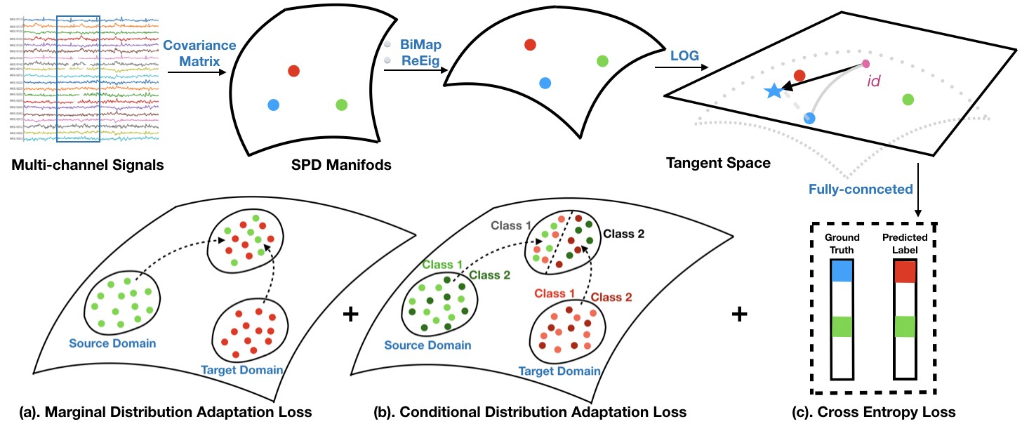
Figure 1: Schematic representation of Deep Optimal Transport employing SPDNet: Multi-channel signals are first transformed into covariance matrices through a pre-established sliding window, situating these matrices on the space of ($\mathcal{S}_{++}$, $g^{LEM}$). Subsequently, the data is processed through Bi-Map, ReEig, and LOG layers, moving it to the tangent space of the SPD manifolds. These neural network layers are proposed by SPDNet. The loss function takes into account the cross-entropy loss, the MDA loss, and the CDA loss.

3.2 Deep Optimal Transport on SPD Manifolds

In this chapter, based on the OT-DA framework on ($\mathcal{S}_{++}$, $g^{LEM}$) discussed in the previous chapter, we propose a deep learning-based domain-adaptation category for the SPD matrix-valued scenario, referred to as the category of Deep Optimal Transport (DOT). Under the assumption that samples from the source and target domains can be restored via OT, the category of DOT capitalizes on deep neural networks on the SPD manifold to extract discriminative information from the SPD matrix-valued features. The network architectures on SPD manifolds consist of the following layers:

• Bi-Map Layer: This layer transforms the covariance matrix $S$ by applying the Bi-Map transformation $W\cdot S\cdot W^{T}$, where the transformation matrix $W$ must have full row rank.

• ReEig Layer: This layer introduces non-linearity to SPD manifolds using $U\cdot\max{(\epsilon I,\Sigma)}\cdot U^{T}$, where $S=U\cdot\Sigma\cdot U^{T}$, $\epsilon$ is a rectification threshold, and $I$ is an identity matrix.

• LOG Layer: This layer maps elements on SPD manifolds to their tangent space using $U\cdot\log{(\Sigma)}\cdot U^{T}$, where $S=U\cdot\Sigma\cdot U^{T}$. The logarithm function applied to a diagonal matrix takes the logarithm of each diagonal element individually.

All of the neural network layers above are proposed in SPDNet [28], which is specifically designed to process SPD matrices, while ensuring their SPD property is maintained across layers during non-linear learning.

After substituting the $\ell_{2}$ distance in Formula 4 with the Riemannian distance, DOT can be seen as a specific variation of the DeepJDOT architecture designed for SPD matrix-valued features. It incorporates an objective function defined as follows:

$$\mathcal{L}(y,f(g(S)))+\sum_{i,j}\gamma_{i,j}\cdot\big{(}d_{g^{LEM}}(g(S),g(\bar{S}))+\mathcal{L}(y,f(g(\bar{S})))\big{)},$$

which likewise results in an alternating parameter update method akin to that of DeepJDOT.

Furthermore, considering that specific conditions in application scenarios can be utilized to simplify transport plans, the DOT framework will encompass several variants. These variants are composed of optimal transport problems that only consider the centroids of class data rather than each individual data point. Keep in mind that under the premise of modelling with Log-Euclidean geometry, we have $X_{S}=X_{T}$, however, $\mathbb{P}_{S}(\varphi(X_{S}))\neq\mathbb{P}_{T}(\varphi(X_{T}))$ and $\mathbb{Q}_{S}(Y_{S}|\varphi(X_{S}))\neq\mathbb{Q}_{T}(Y_{T}|\varphi(X_{T}))$. Hence, DOT will address the more common problems of marginal distribution adaptation and conditional distribution adaptation in application scenarios, specifically on ($\mathcal{S}_{++}$, $g^{LEM}$). The proposed architecture is depicted in Figure 1. Next, we will introduce two distribution adaptation schemes, notably, the calculation for conditional distribution adaptation requires the use of pseudo labels method.

Marginal Distribution Adaptation (MDA) on ($\mathcal{S}_{++}$, $g^{LEM}$): The objective of MDA is to adapt the marginal distributions $\mathbb{P}_{S}(X_{S})$ and $\mathbb{P}_{T}(X_{T})$ on ($\mathcal{S}_{++}$, $g^{LEM}$). We measure the statistical discrepancy between them using the Riemannian distance $d_{g^{LEM}}(\overline{w}(\mathcal{B}_{S}),\overline{w}(\mathcal{B}_{T}))$ between the Log-Euclidean Fr$\acute{e}$chet means of each batch of source and target samples $\mathcal{B}_{S}$ and $\mathcal{B}_{T}$, respectively, as shown in Equation 1. In particular, we formulate the MDA loss as follows,

$$~{}\mathcal{L}_{MDA}:=||\log\big{(}\overline{w}(\mathcal{B}_{S})\big{)}-\log\big{(}\overline{w}(\mathcal{B}_{T})\big{)}||_{\mathcal{F}}.$$ (6)

Conditional Distribution Adaptation (CDA) on ($\mathcal{S}_{++}$, $g^{LEM}$): The objective of CDA is to address the adaptation of conditional distributions $\mathbb{Q}_{S}(Y_{S}|X_{S})$ and $\mathbb{Q}_{T}(Y_{T}|X_{T})$ on ($\mathcal{S}_{++}$, $g^{LEM}$). Following the methodology proposed in [17], we consider class-conditional distribution $\mathbb{Q}(X|Y)$ instead of posterior probability $\mathbb{Q}(Y|X)$ and introduce the use of pseudo labels $\hat{y}$ for the unsupervised setting. To quantify the statistical difference between $\mathbb{Q}_{S}(Y_{S}|X_{S})$ and $\mathbb{Q}_{T}(Y_{T}|X_{T})$, we continue to employ the Riemannian distance $d_{g^{LEM}}(\overline{w}(\mathcal{B}_{S^{\ell}}),\overline{w}(\mathcal{B}_{T^{\ell}}))$ between the Log-Euclidean Fr$\acute{e}$chet means of each batch of source and target samples $S^{\ell}:=\{x_{S}|\hat{y}_{S}={\ell}\}$ and $T^{\ell}:=\{x_{T}|\hat{y}_{T}=\ell\}$, respectively, for class $\ell\in\{1,....,L\}$, as given in Equation 1, i.e.,

$$~{}\mathcal{L}_{CDA}:=||\log\big{(}\overline{w}(\mathcal{B}_{S^{\ell}})\big{)}-\log\big{(}\overline{w}(\mathcal{B}_{T^{\ell}})\big{)}||_{\mathcal{F}}.$$ (7)

In particular, this step necessitates the use of pseudo labels for the target set, which is predicted by a baseline algorithm.

The objective function of the MDA and CDA approach is composed of the cross-entropy loss $\mathcal{L}_{CE}$ and the joint distribution adaptation on ($\mathcal{S}_{++}$, $g^{LEM}$), which includes the loss $\mathcal{L}_{MDA}$ for the marginal distribution adaptation and the loss $\mathcal{L}_{CDA}$ for the conditional distribution adaptation, i.e.,

$$\mathcal{L}_{DOT}:=\alpha_{1}\cdot\mathcal{L}_{CE}+\alpha_{2}\cdot\mathcal{L}_{MDA}^{2}+\alpha_{3}\cdot\mathcal{L}_{CDA}^{2},$$ (8)

where $\alpha_{1},\alpha_{2}$, and $\alpha_{3}\geq 0$. The MDA and CDA losses in Equation 8 must be in the form of squared distance, as required by Brenier’s formulation and Mccann’s results for optimal transport on Riemannian manifolds [38]. These quadratic loss functions are used to induce the neural network to map the source domain and target domain into a common subspace.

DOT does not directly tackle an OT problem. Instead, it leverages the transportation cost as a guiding principle to direct the learning process of the neural network. The trained neural network consequently maps both the source and target domains onto a subspace of the SPD manifold, thus realizing a form of subspace method in transfer learning. We classify DeepJDOT under the DOT umbrella. DeepJDOT computes the transportation cost for all points and require alternating parameter updates, as the transport plan is a deterministic full transfer, whereas the other variants (MDA/CDA) in DOT only calculates this cost for the centroid points and consider the isssue of the conditional marginal adaptation but doesn’t require alternating parameter updates.

Remark.

1). On the space of $\mathcal{S}_{++}$, there are multiple available Riemannian metrics besides LEM. For example, the affine invariant Riemannian metric (AIRM) $g^{AIRM}$ is another well-known Riemannian metric that has been extensively investigated in the literature [23]. However, AIRM is not a suitable choice for our framework. The calculation of the Fr$\acute{e}$chet mean on ($\mathcal{S}_{++}$, $g^{AIRM}$) requires iterative methods, as demonstrated in Formula 9 in the discussion section. This is not feasible as a loss function for deep learning-based approaches.

2). In practice, we substitute Equation 2 into the generalized $\mathcal{L}_{MDA}$ (Equation 6) and $\mathcal{L}_{CDA}$ (Equation 7), resulting in the simplified expressions,

$$\mathcal{L}_{MDA} =||\sum_{S_{i}\in\mathcal{B}_{S}}\frac{\log{(S_{i})}}{|\mathcal{B}_{S}|}-\sum_{S_{j}\in\mathcal{B}_{T}}\frac{\log{(S_{j})}}{|\mathcal{B}_{T}|}||_{\mathcal{F}};$$

$$\mathcal{L}_{CDA} =||\sum_{{S^{\ell}_{i}}\in\mathcal{B}_{S^{l}}}\frac{\log{({S^{\ell}_{i}})}}{|\mathcal{B}_{S^{\ell}}|}-\sum_{{S^{\ell}_{j}}\in\mathcal{B}_{T^{\ell}}}\frac{\log{({S^{\ell}_{j}})}}{|\mathcal{B}_{T^{\ell}}|}||_{\mathcal{F}}.$$

With regard to domain adaptation, these simplified expressions have two distinct interpretations:

First, they can be ssen as an empirical maximum mean discrepancy approach defined as,

$$\mathcal{L}_{MMD}=||\sum_{i=1}^{n}\frac{\varphi{(S_{i})}}{n}-\sum_{j=1}^{m}\frac{\varphi{(S_{i})}}{m}||_{\mathcal{H}},$$

where $n=|\mathcal{B}_{S}|$, $m=|\mathcal{B}_{T}|$, $\varphi{(x)}:=\log{(x)}$ is the feature map, $\mathcal{H}:=\mathbb{R}^{d}$ is the reproducing kernel Hilbert space, and $d$ is the output dimension.

Second, since each matrix $S$ in $\mathcal{B}_{S}$ or $\mathcal{B}_{T}$ is a covariance matrix of multichannel signals, the expressions can also be viewed as a correlation alignment (CORAL) approach [39, 40]. This approach aligns the second-order statistics of the source and target data distributions to minimize the drift between their statistical distributions.

3). For multi-source adaptation, the loss function can be modified by incorporating multi-joint distribution adaptions between each pair of source and target domains on ($\mathcal{S}_{++}$, $g^{LEM}$), as

$$\mathcal{L}:=\alpha_{1}^{i}\cdot\mathcal{L}_{CE}+\sum_{i}\Big{(}\alpha_{2}^{i}\cdot\mathcal{L}_{MDA,i}+\alpha_{3}^{i}\cdot\mathcal{L}_{CDA,i}\Big{)},$$

where the subscript $i$ is used to represent the i-th source domain. This modification is based on the theory of multi-marginal optimal transport on Riemannian manifolds [41] and multi-source joint distribution optimal transport [42].

4 EXPERIMENTS

4.1 Deep Optimal Transport-Based EEG Classifier

In this section, we model the signal spatial covariance matrix that occurs during the motor imagery process in ($\mathcal{S}_{++}$, $g^{LEM}$) and use the proposed framework to address the probelm that signal statistical characterization is shifted during the feedback phase. Given that both Event-Related Desynchronization/Synchronization (ERD/ERS) effects occur during motor imagery process, we can assume that features in the feature space are invariant, i.e., $X_{S}=X_{T}$. Therefore, it is reasonable to model using log-Euclidean geometry. Specificially, in MI-EEG classification, multi-channel EEG signals are represented by $X\in\mathbb{R}^{n_{C}\times n_{T}}$, where $n_{C}$ and $n_{T}$ denote the number of channels and timestamps, respectively. The corresponding spatial covariance matrix, $S:=S(\Delta f\times\Delta t)\in\mathcal{S}_{++}^{n_{C}}$, represents an EEG signal segment within the frequency band $\Delta f$ and time interval $\Delta t$. Let $\mathcal{F}$ and $\mathcal{T}$ represent the frequency and time domains, respectively. We assume the existence of a segmentation $Seg(\mathcal{F},\mathcal{T})$, defined as $\{\Delta f\times\Delta t|\Delta f\subset Range(\mathcal{F})\text{, and }\Delta t\subset Range(\mathcal{T})\}$, on the time-frequency domain of EEG signals. The hypothetical efficacy of the DOT-based MI-EEG classifier in the domain adaptation problem can be seen in the schematic Figure 2. For the theoretical convergence of the proposed computational approach in this real-world context, the following assumptions are necessary:

Assumption 1.

There exists linear transformations between the feature space distributions on the source and target domains for each segment of $Seg(\mathcal{F},\mathcal{T})$, which can be estimated using the discrete Monge-Kantorovich problem 5.

Assumption 2.

The weights for the Log-Euclidean Fr$\acute{e}$chet mean of a batch of samples on each time-frequency segment $\Delta f\times\Delta t\in Seg(\mathcal{F},\mathcal{T})$ in both the source and target empirical distributions are uniform and equal to $1/|Seg(\mathcal{F},\mathcal{T})|$.

Assumption 3.

The Riemannian distance between the Log-Euclidean Fr$\acute{e}$chet means of a batch of source and target samples, both under the same time-frequency segment, is minimized, that is:

$$d_{g^{LEM}}\big{(}\overline{w}(\mathcal{B}_{S}),\overline{w}(\mathcal{B}_{T})\big{)} \leq d_{g^{LEM}}\big{(}\overline{w}(\mathcal{B}_{S}),\overline{w}(\mathcal{B}_{T}^{\prime})\big{)},$$

where $\mathcal{B}_{T}^{\prime}$ is a batch of samples on the target domain that is generated by the other time-frequency segments $\Delta f^{\prime}\times\Delta t^{\prime}\in Seg(\mathcal{F},\mathcal{T})$, where $\Delta f^{\prime}\neq\Delta f$ or $\Delta t^{\prime}\neq\Delta t$.

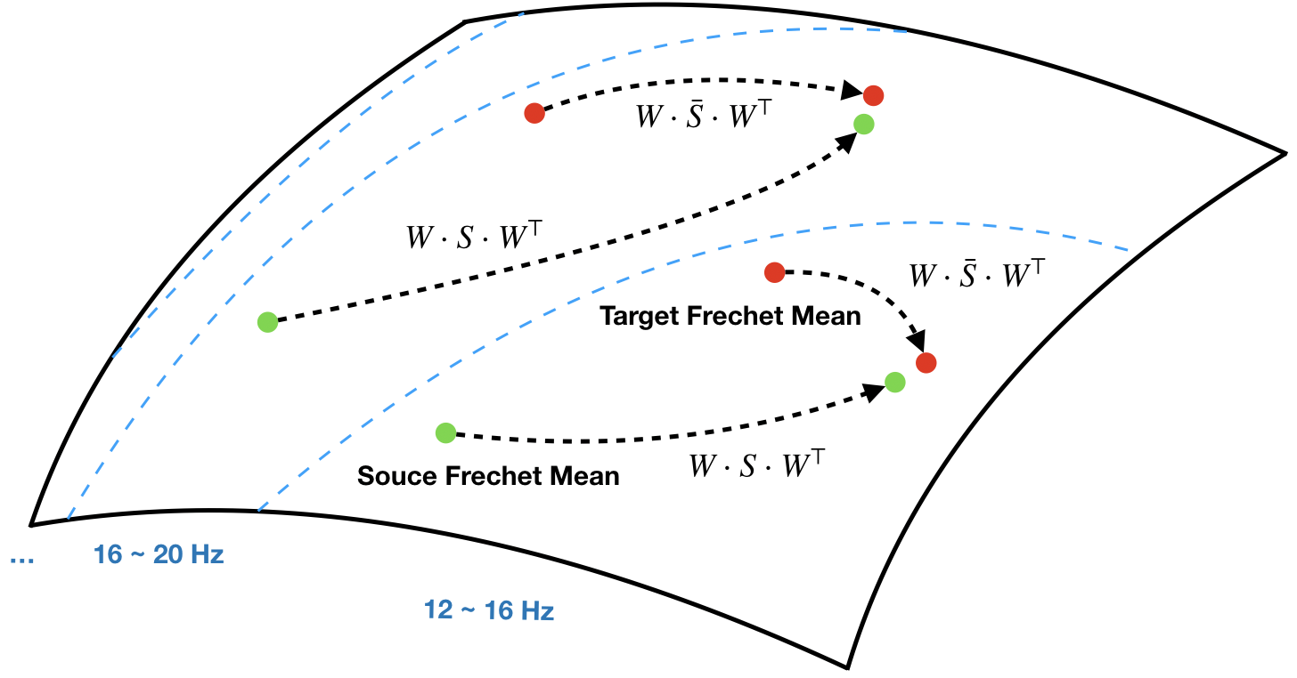
Figure 2: Illustration of DOT-Based Motor-Imagery Classifier: The proposed classifier is with the OD-DA framework on SPD manifolds that simultaneously transports the source and target Fr$\acute{e}$chet means in each frequency band to a common subspace of the same frequency band. Assumption 2 guarantees that each frequency band contributes equally to the classification. Assumption 3 states that each pair of transformations occurs within a frequency band.

Corollary 3.1.

Suppose EEG signals in the source and target domain have the same segmentation, Seg($\mathcal{F},\mathcal{T}$). Assuming we model EEG spatial covariance matrices in ($\mathcal{S}_{++}^{n_{C}}$, $g^{LEM}$) and that Assumption 1,  2, and 3 exist, then the values of the continuous optimal transport $T(S)$ reside within the set $\big{\{}\log(S_{i})\big{\}}_{i=1}^{N}$.

Proof.

In this case, the transport plan $\gamma$ is identity matrix. Theorem 3 directly implies this corollary as Assuption 1 and 2. ∎

Remark.

Assumption 1 is the necessary condition for modelling using the OT problem. Assumption 2 is straightforward because when we are uncertain about which frequency band has a higher weight for a specific task, we tend to assume that each frequency band has equal priority for the classification task. Assumption 3 is set based on the inspiration from practical problems as the frequency band $\Delta f$ is often discretized according to its physiological meaning, such as $\delta$ (less than 4 Hz), $\theta$ ($4\sim 7$ Hz), $\alpha$ ($8\sim 13$ Hz), $\beta$ ($14\sim 30$ Hz), and $\gamma$ (above 30 Hz) activity. This assumption ensures that features extracted from different frequency bands do not intersect with each other.

4.2 Evaluation Dataset

As part of our evaluation, we utilized three commonly used motor imagery datasets. This section provides a brief overview of these datasets. The data from these datasets cannot be accessed via MOABB or BNCI Horizon 2020. The selection criteria for the three evaluation datasets from MOABB and BNCI Horizon 2020 require that each subject has two-session recordings that were collected on different days. All digital signals were filtered using Chebyshev Type II filters at intervals of 4 Hz. The filters were designed to have a maximum loss of 3 dB in the passband and a minimum attenuation of 30 dB in the stopband. The followings are the descriptions of these three datasets.

Korea University Dataset (KU): The KU dataset (also known as Lee2019_MI in MOABB) comprises EEG signals obtained from 54 subjects during a binary-class EEG-MI task. The EEG signals were recorded using 62 electrodes at a sampling rate of 1,000 Hz. For evaluation, we selected 20 electrodes located in the motor cortex region, specifically FC-5/3/1/2/4/6, C-5/3/1/z/2/4/5, and CP-5/3/1/z/2/4/6. The dataset was divided into two sessions, S1 and S2, each consisting of a training and a testing phase. Each phase included 100 trials, with an equal number of right and left-hand imagery tasks, resulting in a total of 21,600 trials available for evaluation. The EEG signals were epoched from second 1 to second 3.5 relative to the stimulus onset, resulting in a total epoch duration of 2.5 seconds.

BNCI2014001: The BNCI2014001 dataset (also known as BCIC-IV-2a) involved 9 participants performing a motor imagery task with four classes: left hand, right hand, feet, and tongue. The task was recorded using 22 Ag/AgCl electrodes and three EOG channels at a sampling rate of 250 Hz. The recorded data were filtered using a bandpass filter between 0.5 and 100 Hz, with a 50 Hz notch filter applied. The study was conducted over two sessions on separate days, with each participant completing a total of 288 trials (six runs of 12 cue-based trials for each class). The EEG signals were epoched from the cue onset at second 2 to the end of the motor imagery period at second 6, resulting in a total epoch duration of 4 seconds.

BNCI2015001: The investigation of BNCI2015001 involved 12 participants performing a sustained right-hand versus both-feet imagery task. Most of the study consisted of two sessions conducted on consecutive days, with each participant completing 100 trials for each class, resulting in a total of 200 trials per participant. Four subjects participated in a third session, but their data were not included in the evaluation. The EEG data were acquired at a sampling rate of 512 Hz and filtered using a bandpass filter ranging from 0.5 to 100 Hz, with a notch filter at 50 Hz. The recordings began at second 3 with the prompt and continued until the end of the cross period at second 8, resulting in a total duration of 5 seconds.

4.3 Experimental Settings

The experimental settings for domain adaptation on the three evaluated datasets are described as follows and illustrated in Figure 3: 1). Semi-supervised Domain Adaptation: For the KU dataset, Session 1 was used for training, and the first half of Session 2 was used for validation, while the second half was reserved for testing. Early stopping was adopted during the validation phase. 2). Unsupervised Domain Adaptation: For the BNCI2014001 and BNCI2015001 dataset, Session 1 was used for training, and Session 2 was used for testing. No validation set was used, and a maximum epoch value (e.g., 500) was set for stopping in practice.

We specified that knowledge transfer must always occur from Session 1 (source domain) to Session 2 (target domain), i.e., $S1\longrightarrow S2$ for each dataset. This is because there is no neurophysiological meaning if negative transfer is used in the learning process. Typically, the former and latter sessions correspond to the calibration and feedback phases.

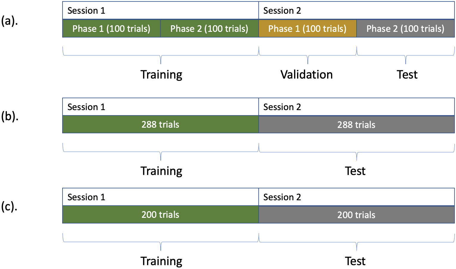
Figure 3: Illustrations for experimental settings on three datasets: (a). KU; (b). BNCI2014001; (c). BNCI2015001

4.4 Evaluated Baselines

In this article, we solely focus on geometric methods, which are based on EEG spatial covariance matrices, as comparative methods in the MI-EEG cross-session scenario. These methods can be broadly divided into four categories. These include the Category of Parallel Transportation (PT), Category of Deep Parallel Transportation (DPT), the Category of Optimal Transport, and the Category of Deep Optimal Transport. Each category encompasses various transfer methods, constructed on the foundation of three types of classifiers: the support vector machine (SVM), Minimum Distance to Riemannian Mean (MDM), and SPDNet. We begin by introducing these three classifiers, followed by a discussion of the transfer methods within each category.

1. Support Vector Machine (SVM) [43]: SVM is a well-known machine learning classifier used for classification and regression tasks, which aims to find an optimal hyperplane that maximally separates data points of different classes, allowing it to handle linear and non-linear classification problems effectively. After extracting features from EEG signals, they are fed into an SVM classifier for classification purposes.

2. Minimum Distance to Riemannian Mean (MDM) [13]: MDM employs the geodesic distance on ($\mathcal{S}_{++}$, $g^{AIRM}$), which comprises EEG spatial covariance matrices, as a prominent feature in the classification phase of a feature-engineering procedure. More specifically, a centroid is estimated for each predefined class, and subsequently, the classification of a new data point is determined based on its proximity to the nearest centroid.

3. SPDNet: The network architecture of SPDNet has been elaborated in Section 3.2. In the experiments, we only use one Bi-Map layer, with both the input and output dimensions equal to the number of motor imagery cortical electrodes: 20 for the KU dataset, 22 for the BNCI2014001 dataset, and 13 for the BNCI2015001 dataset.

In the subsequent section, we will classify the transfer methods on the SPD manifold. As some of these methods involve computations related to Riemannian metrics, we will emphasize the specific Riemannian metrics associated with each method. In the present work, the Riemannian metrics on the SPD manifold only include $g^{AIRM}$ and $g^{LEM}$. The different transfer methods across the four categories according to the Riemannian metric can be seen in the first three columns of Table II.

4.4.1 Category of Parallel Transportation

This category refers to the utilization of parallel transport on manifolds to perform transfer of training and testing data. Specifically, on ($\mathcal{S}_{++}$, $g^{LEM}$), parallel transport is an identity mapping, and therefore methods based on parallel transport for transfer learning are modeled using $g^{AIRM}$. One of the representative methods in this context is called Riemannian Procrustes Analysis (RPA) [44]. RPA utilizes transformations on ($\mathcal{S}_{++}$, $g^{AIRM}$), including translation, scaling, and rotation. After the geometric transformation, RPA uses the MDM approach as the base classifier. The RPA approach includes three sequential processes: recentering (RCT), stretching, and rotation (ROT). First, the RCT process is used to re-centralize the centroids of the data to the identity matrix. In implementation, ROT is the parallel transportation on ($\mathcal{S}_{++}$, $g^{AIRM}$) from the Fr$\acute{e}$chet mean of either source domain or target domain to the identity matrix. Second, the stretching process rescales the distributions on both datasets so that their dispersions around the mean are the same. Finally, the ROT process rotates the matrices from the target domain around the origin and matches the orientation of its point cloud with that of the source domain. In particular, the ROT process is unsupervised and can be used in unsupervised domain adaptation, whereas the RCT process is supervised and can only be used in semi-supervised domain adaptation. Specifically, RCT was proposed as a standalone method in [45] to address the MI-EEG classification problem.

4.4.2 Category of Deep Parallel Transportation

This category also refers to source-target domain transfer on the SPD manifold using parallel transportation. However, this category is coupled with deep neural networks on the SPD manifold. The representative work of this category is known as Riemannian Batch Normalization (RieBN) [46]. RieBN is an SPD matrix-valued network architecture that employs parallel transport for batch centering and biasing on SPD neural networks. The efficacy of this network structure, as well as its further optimized approach, has been validated on multiple MI-EEG classification datasets [31, 33]. Specifically, when referring to the RieBN method, we always assume that the Riemannian metric is $g^{AIRM}$.

4.4.3 Category of Optimal Transport

This category refers to treating the distribution of the covariance matrix obtained from cross-session as an OT problem and solving the transportation plan using different variants of Wasserstein distances [47]. The classifier is trained within a session and tested in a shifted session. This is an unsupervised method. We offer three different types of Wasserstein distances, including the earth mover’s distance (EMD) on either ($\mathcal{S}_{++}$, $g^{LEM}$) or on ($\mathcal{S}_{++}$, $g^{AIRM}$), Sliced-Wasserstein distance (SPDSW), and Log Sliced-Wasserstein distance (logSW).

4.4.4 Category of Deep Optimal Transport

This category pertains to the approach proposed in this paper, which uses SPD neural networks on ($\mathcal{S}_{++}$, $g^{LEM}$) to transfer both marginal distribution and conditional distribution, migrating the source domain and target domain to a common space induced by optimal transport. Within this category, the methods we propose include MDA, CDA, and MDA+CDA. As discussed in the introduction section, we will also include the DeepJDOT methodology within this category.

5 Main Results

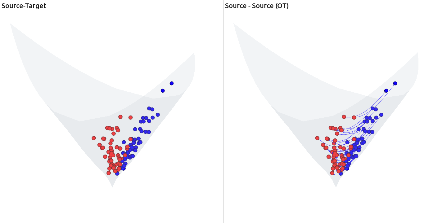
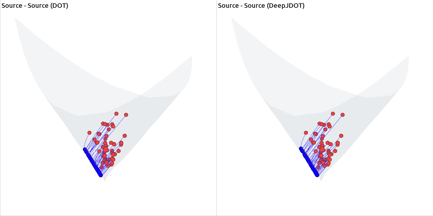
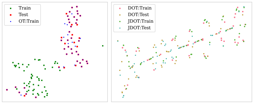
Figure 4: Synthetic Dataset on cone of the 2-dimensional ($\mathcal{S}_{++}$, $g^{LEM}$): The panels from left to right and top to bottom are sequentially labeled as (a) to (f). In panels (a) to (d), the red data points represent the source domain, while the blue data points indicate their locations after the algorithmic transformation. The x-axis and y-axis of Panels (e) and (f) represent two eigenvalues of the covariance matrix respectively. The two figures are designed to observe the distribution on a plane constituted by matrix eigenvalues after the transfer by these methods.

TABLE II: Comparative experiment table for three public datasets: All results in the table are in percentages (%), and the comparison methods include four categories, nine methods, and the corresponding three base classifiers. The original results of the base classifiers without considering transfer methods are at the bottom of the table. In the table, we use the symbol "/" to indicate that this method does not exist in the scenario constructed by this dataset.

Metric of $\mathcal{S}_{++}$	Category	Method	Classifier	KU (54 Subjects)		BNCI2014001 (9 Subjects)		BNCI2015001 (12 Subjects)
				$S1\longrightarrow S2$		$T\longrightarrow E$		$S1\longrightarrow S2$
				Semi-supervised		Unsupervised		Unsupervised
				Accuracy	Increment	Accuracy	Increment	Accuracy	Increment
$g^{AIRM}$	OT	EMD	SVM	65.24 (14.81)	$-$0.07	50.89 (16.54)	$-$14.27	82.17 (11.80)	$+$6.25
	PT	RCT	MDM	52.69 (6.39)	$+$0.34	55.13 (12.48)	$+$0.89	77.67 (13.23)	$+$5.46
		ROT	MDM	51.39 (5.89)	$-$0.96	/
		RCT	SPDNet	69.91 (13.67)	$+$2.15	72.11 (12.99)	$+$3.51	81.25 (10.64)	$+$4.75
		ROT	SPDNet	63.44 (14.94)	$-$4.32	/
	DPT	RieBN	SPDNet	67.57 (15.27)	$-$0.19	69.33 (13.49)	$+$0.73	78.83 (14.56)	$+$2.33
$g^{LEM}$	OT	EMD	SVM	67.70 (15.14)	$-$0.06	68.44 (15.79)	$+$3.28	82.17 (11.80)	$+$6.25
		EMD	SPDNet	64.22 (14.30)	$-$3.54	62.15 (14.69)	$-$6.45	78.33 (13.80)	$+$1.83
		SPDSW	SVM	66.67 (14.54)	$+$1.36	67.82 (16.71)	$+$2.66	82.42 (11.74)	$+$6.50
		logSW	SVM	66.26 (15.00)	$+$0.95	65.82 (16.56)	$+$0.66	80.75 (12.94)	$+$4.83
	DOT	DeepJDOT	SPDNet	67.38 (14.67)	$-$0.38	61.00 (11.40)	$-$7.60	77.63 (15.12)	$+$1.13
		MDA	SPDNet	69.19 (14.37)	$+$1.43	67.78 (12.46)	$-$0.82	78.33 (14.57)	$+$1.83
		CDA	SPDNet	68.80 (14.29)	$+$1.04	65.12 (11.34)	$-$3.48	78.25 (14.59)	$+$1.75
		MDA+CDA	SPDNet	68.61 (14.79)	$+$1.05	64.85 (11.54)	$-$3.75	78.29 (11.99)	$+$1.79
			SVM	65.31 (14.42)		65.16 (17.00)		75.92 (16.29)
Base Classifier			MDM	52.35 (6.73)		54.24 (13.31)		72.21 (14.67)
			SPDNet	67.76 (14.55)		68.60 (13.03)		76.50 (14.41)

5.1 Synthetic Dataset

In this experiment, we synthesize a source domain dataset consisting of 50 covariance matrices of size $2\times 2$, drawn from a Gaussian distribution on the SPD manifold [48] with a median of 1 and a standard deviation of 0.4. We utilize a transformation matrix $W=[[1,0.5],[0.5,1]]$, such that data in the target domain is expressed as $W\cdot S\cdot W^{\top}$.

Figure (a) exhibits red points sourced from the source domain, with the blue points originating from the target domain. In Figure (b), the blue points represent the relocation of the red points via the Earth Mover’s Distance (EMD) method from Optimal Transport (OT). The associations made by this transformation are represented by thin blue lines. Remarkably, the position of these transformed blue points is extremely proximate to the points of the target domain in Figure (a). This can be attributed to the fact that the OT-DA method essentially computes a weighted average of the original source and target domain data points, based on weights learned to maximize the transportation cost. As such, in Figure (e), we observe numerous transformed blue points enveloped by the yellow points from the target domain.

The transformed blue points in Figures (c) and (d) were derived from mapping the red points via neural network weights learned through the DOT and DeepJDOT methods, respectively. Corresponding point pairs are linked with thin blue lines. These figures reveal the shared fundamental characteristic of the DOT and DeepJDOT methods that both project the source and target domains onto a subspace learned via a network, which, in these two figures, is represented by a straight line. In the context of differential geometry, this indeed represents a form of submanifold. A submanifold refers to a lower-dimensional manifold embedded within a higher-dimensional one. In this case, the 2D matrices are being represented by a 1D line, essentially projecting the higher dimensional data onto a lower dimensional space. This reduces the complexity of the data while preserving key information. Furthermore, as indicated by Figure (f), this subspace is even identical for both methods.

5.2 Comparative Experiments on Real-World EEG Datasets

As shown in Table II, we classify the $\mathcal{S}_{++}$ space into three categories according to different Riemannian metrics. The first category does not require computation using a Riemannian metric, the second employs $g^{AIRM}$, while the third uses $g^{LEM}$. As the experimental results indicate, considering different metrics is necessary. For instance, in the table, EMD+SVM achieved 50.89 ($g^{AIRM}$) and 68.33 ($g^{LEM}$) respectively on the BNCI2014001 dataset.

First, we introduce several observations: 1). The improvement is related to the number of participants. On two datasets with fewer participants (i.e., BNCI2014001/BNCI2015001), the enhancement brought by the transfer methods is more significant. We noticed several scenarios where there was an increase or decrease of more than 5%. 2). The extent of improvement is related to the base classifier’s results. If the results from the base classifier are low, then there are more opportunities for the transfer methods to achieve significant improvements. 3). All the improved results are related to the structure of the classifier neural network, the selection of test parameters, the preprocessing of datasets, and so on. Therefore, the conclusions of this study may not necessarily be universally applicable.

Next, we compare the methods in different spaces as follows:

• ($\mathcal{S}_{++}$, $g^{AIRM}$) includes three categories (Cat. OT, PT & DPT). Combining the results from all three datasets, the RCT method in Cat. PT performs well when paired with the MDM or SPDNet classifier. The EMD method in Cat. OT has the largest variation in performance. It is worth noting that although the second step ROT in the RPA method can only be used in semi-supervised domain adaptation scenarios, its performance is noticeably worse than RCT, which is consistent with the results reported in their original paper. The RieBN method in Cat.DPT slightly improves the results, but all three performances are weaker than the RCT method.

• ($\mathcal{S}_{++}$, $g^{LEM}$) includes two categories (Cat. OT and DOT). The EMD method paired with the SVM classifier performs significantly better than when paired with the SPDNet classifier. SPDSW and logSW methods have obvious improvements compared to their base classifier (SVM), among which SPDSW performs better than logSW by 1 to 2 percentage points on all three datasets. The methods based on MDA and CDA proposed in this paper perform very closely, except for the BNCI2014001 dataset, the improvements on the other two datasets are between 1 to 2 percent, where the MDA method is slightly better than CDA or a mixture of MDA and CDA. Notably, the pseudo-label method was used in the use of CDA methods. The accuracy of the pseudo-label will affect the final result. DeepJDOT shares certain similarities with the method we propose; However, its performance across three datasets falls short of our proposed approach. The primary reason for this could be attributed to our decision to replace the task of computing transportation costs for each data point with merely computing transportation costs for the centers of each frequency band’s dataset. For classification tasks, minimizing the transportation cost does not necessarily imply improved accuracy, thus this alteration reduces computational overhead while enhancing the model’s potential.

Comparing methods across different spaces, numerically, the RieBN method and the DOT methods proposed in this paper are quite close, but weaker than the RCT method. Compared to other Cat. OT methods (EMD/SPDSW/logSW), the deep learning-based approaches results in a higher overall classification outcome. When it comes to the calculation of CDA in DOT, we employed the pseudo label method. These pseudo labels come from the classification results of the Geometric EEG Classifiers in [32], which currently yields the best performance on subject-specific tasks. Although more accurate pseudo labels would enhance the performance of DOT, we cannot expect superior techniques to be currently available. Specifically, the results of SPDSW and logSW on BNCI2014001 are obtained by invoking the filters provided by the author in the corresponding GitHub repository of the article, which perform much better than our more rudimentary filters. This is because the decoding performance of traditional machine learning methods relies heavily on the selection of handcrafted features.

Overall, these geometric transfer methods are effective. However, it is important to note that these tasks are often employed for testing transfer learning methods as domain shift is known to exist. However, the performance degradation of classifiers on these tasks is not solely due to the domain shift, hence any improvements offered by transfer learning methods are inherently limited. Additionally, we currently lack an effective method to quantify the intensity of domain shift, thus we are unable to fully quantify the performance of these methods. Therefore, these results are merely observations in these constrained scenarios. In addition, the results can be also significantly influenced by various factors, such as the choice of classifier, dataset settings, and the architecture of the methods themselves. We prefer not to provide further insights based solely on these numerical results, as they may not capture the full picture.

6 DISCUSSIONS

In this section, we will summarize and discuss the ambiguity and limitations of DOT in the following issues.

6.1 Integration with Geometric EEG Classifiers

We naturally integrate the proposed Category DOT into the Geometric EEG Classifiers, such as Tensor-CSPNet [31] and Graph-CSPNet [32]. It’s important to note that the Geometric EEG Classifiers operate on $g^{AIRM}$, so when we select this classifier, we need to disable the RieBN layer and change all operations involving the Riemannian distance to be computed under $g^{LEM}$. It is worth emphasizing that the classification results from the slected network architecture are not optimal. The architecture for all experiments consists of a single BiMap layer, ensuring that the number of input and output units match the number of electrodes in the motor cortex. There is a certain gap compared with the classification results using SPDNet to construct Geometric EEG Classifiers. However, such simplification is intended to highlight the improvement effect of transfer and not to be disturbed by the maximum relevant information contained in the data related to classification.

TABLE III: Table for several operators on SPD manifolds under $g^{AIRM}$ and $g^{LEM}$. $D\log$ and $D\exp$ are the Fr$\acute{e}$chet derivatives of the principal matrix logarithm $\log$ and the matrix exponential map $\exp$ respectively.

	$g^{AIRM}$	$g^{LEM}$
Inner product: $\langle S_{1},S_{2}\rangle_{P}$	$\operatorname{Tr}{(P^{-1}\cdot S_{1}\cdot P^{-1}\cdot S_{2}})$	$\langle D\log{(P)}(S_{1}),D\log{(P)}(S_{2})\rangle$
Riemannian Exponential: $\exp_{P}(S)$	$P^{\frac{1}{2}}\cdot\exp{\big{(}P^{-\frac{1}{2}}\cdot S\cdot P^{-\frac{1}{2}})}\cdot P^{\frac{1}{2}}$	$\exp{\big{(}\log{(P)}+D\log{(P)}(S)\big{)}}$
Riemannian Logarithm: $\log_{P}(S)$	$P^{\frac{1}{2}}\cdot\log{\big{(}P^{-\frac{1}{2}}\cdot S\cdot P^{-\frac{1}{2}})}\cdot P^{\frac{1}{2}}$	$D\exp{\big{(}\log{(P)}\big{)}}\big{(}\log{(S)}-\log{(P)}\big{)}$
Riemannian Geodesic: $\gamma_{t}(S_{1},S_{2})$	$S_{1}^{\frac{1}{2}}\cdot\exp{\big{(}t\cdot\log{(S_{1}^{-\frac{1}{2}}\cdot S_{2}\cdot S_{1}^{-\frac{1}{2}})}\big{)}}\cdot S_{1}^{\frac{1}{2}}$	$\exp{\big{(}(1-t)\cdot\log{(S_{1})}+t\cdot\log{(S_{2})}\big{)}}$
Riemannian Distance: $d_{g}(S_{1},S_{2}$)	$||\log{(S_{1}^{-\frac{1}{2}}\cdot S_{2}^{\frac{1}{2}}\cdot S_{1}^{-\frac{1}{2}})}||$	$||\log{(S_{1})}-\log{(S_{2})}||$
Fr$\acute{e}$chet Mean: $\overline{w}(\mathcal{B})$	$\arg\min_{\mu\in\mathcal{S}_{++}}\sum_{i=1}^{N}d_{g^{AIRM}}^{2}(S_{i},\mu)/N$	$\exp{\big{(}\frac{1}{|\mathcal{B}|}\cdot\sum_{i}\log{(S_{i})}\big{)}}$

6.2 Theorem 3 with cost function $c(x,\bar{x})=||x-\bar{x}||_{\ell^{2}}^{2}$

In this section, we will show Theorem 3 with cost function $c(x,\bar{x})=||x-\bar{x}||_{\ell^{2}}^{2}$ is equilvant to [6, Theorem 3.1]. It was first observed and proved by Yair et al.[10] who use the matrix vectorization operator to establish an isometry between the affine transformation and the Bi-Map transformation. We follow their arguments and revise a bit of their proof.

Theorem 4.

[6, Theorem 3.1]  Let $\mu$ and $\nu$ be two discrete distributions on $\mathbb{R}^{n}$ with $N$ Diracs. Given a strictly positive definite matrix $A$, bias weight $b\in\mathbb{R}^{n}$, and source samples $\{x_{i}\}_{i=1}^{N}\sim\mu$, suppose target samples $\bar{x}_{i}:=A\cdot x_{i}+b$, for $i=1,...,N$, and the weights in both source and target distributions’ empirical distributions are $1/N$. Then, transoport $T(x_{i})=A\cdot x_{i}+b$ is the solution to the OT Problem provided with a cost function $c(x,\bar{x}):=||x-\bar{x}||_{\ell^{2}}^{2}$.

To expose the relationship between the Bi-Map transformation in Theorem 3 and affine transformation in Theorem 4, we introduce the matrix vectorization operator $vec(\cdot)$ to stack the column vectors of matrix $A=(a_{1}\big{|}a_{2}\big{|}\cdots\big{|}a_{n})$ below on another as follows,

$$vec(A):=\begin{pmatrix}a_{1}\\ a_{2}\\ \vdots\\ a_{n}\\ \end{pmatrix}$$

Then, we have the following lemma.

Lemma 5.

$vec(W\cdot S\cdot W^{\top})=(W\otimes W)\cdot vec(S)$, where $\otimes$ is Kronecker product.

Proof.

Suppose $S$ is an $n\times n$ matrix, and $W^{\top}=(w_{1}^{\top}|w_{2}^{\top}|\cdots|w_{m}^{\top})$ is the transpose of $m\times n$ matrix $W$ with each column vector $w_{i}^{\top}\in\mathbb{R}^{n}$ (i=1, …, m). The k-th column vector of $W\cdot S\cdot W^{\top}$ can be written as $(W\cdot S\cdot W^{\top})_{(:,k)}=W\cdot S\cdot w_{k}^{\top}=(w_{k}^{\top}\otimes W)\cdot vec(S)$. Hence, we achieve the lemma as follows,

$$vec(W\cdot S\cdot W^{\top}) =\begin{pmatrix}(W\cdot S\cdot W^{\top})_{(:,1)}\\ \vdots\\ (W\cdot S\cdot W^{\top})_{(:,m)}\\ \end{pmatrix}$$

$$=\begin{pmatrix}w_{1}^{\top}\otimes W\\ \vdots\\ w_{m}^{\top}\otimes W\\ \end{pmatrix}\cdot vec(S)$$

$$=(W\otimes W)\cdot vec(S).$$

∎

Lemma 6.

Suppose $W\in\mathbb{R}^{n\times n}$ is positive definite, then $W\otimes W$ is also positive definite.

Proof.

This is given by a basic fact that suppose $\{\lambda_{1},...,\lambda_{n}\}$ are the eigenvalues of $W$, then the eigenvalues for $W\otimes W$ is $\{\lambda_{1}^{2},...,\lambda_{n}^{2}\}$. Hence, $W\otimes W$ is positive definite. ∎

According to Lemma 5 and 6, the Bi-Map transformation $W\cdot S\cdot W^{\top}$ turns to be affine transformation $A=W\otimes W$, and thus Theorem 3. Hence, Theorem 3 endowed with the cost function $c\big{(}vec(x),vec(y)\big{)}=||vec(x)-vec(y)||_{\ell^{2}}^{2}$ is equilvant to Theorem 4.

6.3 Riemannian Metrics for SPD Manifolds

To allow us to measure distances, angles, and lengths of curves on the smooth manifold, the metric called Riemannian metric is introduced, which is a smoothly varying assignment of inner products to tangent spaces of a smooth manifold and turns the smooth manifold into a Riemannian manifold $(\mathcal{M},g)$. A Riemannian metric $g$ at any $p\in\mathcal{M}$ is a smooth assignment of an inner product $g_{p}:T_{p}\mathcal{M}\times T_{p}\mathcal{M}\longmapsto\mathbb{R}$ to each tangent space $T_{p}\mathcal{M}$, such that for any $u,v\in T_{p}\mathcal{M}$, the following properties hold:

• Positive-definiteness: $g_{p}(u,u)\geq 0$ and $g_{p}(u,u)=0$ if and only if $u=\boldsymbol{0}$.

• Symmetry: $g_{p}(u,v)=g_{p}(v,u)$.

Moreover, we make the assumption that $g_{p}$ exhibits smooth variation. This implies that given any two smooth vector fields $X$ and $Y$, the inner product $g_{p}(X|_{p},Y|_{p})$ is a smooth function of $p$. If we treat the space of SPD matrices as a vector space endowed with standard additive matrix structure, numerous standard operations on SPD matrices turn out to be non-convex and yield matrices which are not positively definite. Indeed, gradient descent, when conducted using the conventional Frobenius norm, fundamentally involves progression along a line within the vector space of symmetric matrices. As a result, one side of this line inevitably intersects the boundary of the cone. Therefore, in Diffusion Tensor Images, a number of authors have concurrently suggested the employment of Riemannian metrics over the space of SPD matrices. These metrics possess the remarkable characteristic of invariance under affine transformations of the base space coordinates [51, 52]. This Riemannian metric on $\mathcal{S}_{++}$ is now referred to as $g^{AIRM}$ and is defined as follows:

$$g^{AIRM}(v,w):=\langle\,P^{-\frac{1}{2}}vP^{-\frac{1}{2}},P^{-\frac{1}{2}}wP^{-\frac{1}{2}}\,\rangle,$$

where $v,w\in T_{P}\mathcal{S}_{++}$. The space of SPD matrices, when endowed with $g^{AIRM}$, transforms into a space characterized by non-positive sectional curvature without the cut-locus, which is globally diffeomorphic to Euclidean space, a manifold known as a Cartan-Hadamard manifold. The Cartan-Hadamard manifold exhibits numerous advantageous geometric and statistical properties when applied to SPD manifolds, such as the uniqueness of geodesics connecting any two SPD matrices and the existence and uniqueness of the mean for a set of SPD matrices, among others. As a result, the structure obtained exhibits many characteristics of Euclidean spaces, despite retaining its manifold structure due to its curvature. Nevertheless, algorithms operating on SPD manifolds endowed with $g^{AIRM}$ tend to exhibit slow performance due to the complexity of matrix computations. To rectify this constraint and concurrently mitigate the swelling effect, Arsigny introduced the Riemannian metric $g^{LEM}$. The chief distinguishing advantage of $g^{LEM}$ is its facilitation of the statistical analysis of SPD matrices, making it much more manageable. Indeed, the log-Euclidean metric $g^{LEM}$ leads to a considerable improvement in computational efficiency, as evidenced by a decrease in computation time by a factor of 4 to 10. When the distance of the data from the identity matrix falls below the Ricci curvature, it is reasonable to affirm that the log-Euclidean framework serves as an effective first-order approximation of affine-invariant computations [24]. In particular, while the Fr$\acute{e}$chet mean of ($\mathcal{S}_{++}$, $g^{LEM}$) possesses an explicit formula, ($\mathcal{S}_{++}$, $g^{AIRM}$) does not. Formally, given a set of SPD matrices $\{S^{1},\cdots,S^{N}\}$, the Fréchet mean $\mu$ [23] of that set is given as follows,

$$\mu:=\arg\min_{\mu\in\mathcal{S}_{++}}\frac{1}{N}\cdot\sum_{i=1}^{N}~{}d_{g^{AIRM}}^{2}(S^{i},\mu).$$

It is implicitly computed through a barycentric equation and solved iteratively as follows:

$$~{}\mu_{t+1}\longleftarrow\mu_{t}^{\frac{1}{2}}\exp{\Big{(}\frac{\sum_{i}\log{(\mu_{t}^{-\frac{1}{2}}S_{i}\mu_{t}^{-\frac{1}{2}})}}{|\mathcal{B}|}\Big{)}}\mu_{t}^{\frac{1}{2}},$$ (9)

where $|\mathcal{B}|$ is the batch size. In Table III, we present the explicit formulations of functions defined on SPD manifolds under two distinct metrics. In recent years, some more advantageous metrics for SPD matrices have been proposed, such as Thompson’s metric [53]. However, these are not considered in the scope of this work.

6.4 Parallel Transportation

Parallel transport is a fundamental concept in Riemannian geometry. On a Riemannian manifold, parallel transport involves the transfer of a tangent vector at one point along a curve on the manifold to another point, such that the transported vector remains parallel to the original vector with respect to the Riemannian metric. This provides a method for comparing tangent vectors at different points on the manifold, allowing for the transmission of information along a continuous path while preserving certain geometric properties. For the two commonly used Riemannian metrics on SPD manifolds, namely $g^{AIRM}$ and $g^{LEM}$, distinct parallel transport expressions are exhibited. Formally, let’s consider $S_{1},S_{2}$ $\in$ ($\mathcal{S}_{++}$, $g^{AIRM}$); the parallel transport from $S_{1}$ to $S_{2}$ for $s\in T_{S_{1}}\mathcal{S}_{++}$ is expressed as

$$\Gamma_{S_{1}\rightarrow S_{2}}(s)=E\cdot s\cdot E^{\top},$$

where $E=(S_{1}\cdot S_{2}^{-1})^{\frac{1}{2}}$. This proposition is proved in [54] and revised in [10]. Conversely, in the case of $g^{LEM}$, assuming $S_{1},S_{2}\in$ ($\mathcal{S}_{++}$, $g^{LEM}$), the parallel transport is given by $\Gamma_{S_{1}\rightarrow S_{2}}(s)=s$. In MI-EEG classifiers, tangent vectors on SPD manifolds are often considered as features of the classifier. Consequently, the distinct parallel transport expressions determine the modeling approaches based on the two different Riemannian metrics: For models employing $g^{AIRM}$, features from different sessions are considered to exhibit a shift, i.e., $X_{S}\neq X_{T}$. Therefore, supervised or unsupervised non-linear transformations are utilized to migrate features from one session to another. This migration operation is generally applied prior to the classifier. In contrast, models based on $g^{LEM}$ assume that features from different sessions do not exhibit a shift, i.e., $X_{S}=X_{T}$. As a result, a single geometric neural network is directly employed for training and testing purposes. These different approaches to modeling based on the chosen Riemannian metric have implications for the overall performance and suitability of the MI-EEG classifier in various scenarios.

7 Justification of Assumption 3

In this section, we will demonstrate through statistical results that Assumption 3 in DOT-based MI-EEG classifier is a reasonable assumption for the MI-BCI dataset. From Table IV of the following page, the numbers on the diagonal represent the Riemannian distances under Log-Euclidean geometry within the same frequency band, which are consistently the smallest among all the row numbers in the two datasets. This suggests that the mapping moves the center of each frequency band in the source domain to the same frequency band center in the target domain.

The procedure of the calculation is as follows: assuming source and target samples can be represented in the format:

$$\text{[trials, frequency bands, channels, channels]},$$

with the frequency bands fixed (in the second dimension), we can first calculate the Fréchet mean. This involves averaging all covariance matrices along the trials dimension, resulting in a shape of [frequency bands, channels, channels]. Next, we can directly compute the log-Euclidean distance for each pair of frequency bands.

In this study, digital signals were filtered using Chebyshev Type II filters at intervals of 4 Hz. The filters were designed to have a maximum loss of 3 dB in the passband and a minimum attenuation of 30 dB in the stopband. This calculation process aligns with intuition. The difference between the same frequency bands should be smaller since they capture similar signal characteristics within the same frequency range. On the other hand, the difference between different frequency bands tends to be larger because they may correspond to distinct signal features or frequency components. Therefore, by computing the difference between frequency bands, we can quantify their dissimilarity in terms of covariance structures.

TABLE IV: Average Log-Euclidean distance between the Fr$\acute{e}$chet means of EEG spatial covariance matrices generated from the different frequency band of the source and target domains on KU (54 subjects), BNCI2014001 (9 subjects), and BNCI2015001 (12 subjects). The shortest distance in each row is highlighted in boldface.

KU: S1 $\backslash$ S2	4$\sim$8 Hz	8$\sim$12 Hz	12$\sim$16 Hz	16$\sim$20 Hz	20$\sim$24 Hz	24$\sim$28 Hz	28$\sim$32 Hz	32$\sim$36 Hz	36$\sim$40 Hz
4$\sim$8 Hz	4.69	4.98	5.82	6.74	7.19	7.64	8.17	8.78	9.28
8$\sim$12 Hz	5.09	4.21	4.82	5.81	6.25	6.70	7.22	7.82	8.31
12$\sim$16 Hz	5.84	4.76	4.01	4.62	4.98	5.34	5.78	6.30	6.75
16$\sim$20 Hz	6.66	5.61	4.37	3.96	4.08	4.33	4.64	5.02	5.40
20$\sim$24 Hz	7.08	6.01	4.66	3.97	3.86	3.99	4.27	4.63	4.97
24$\sim$28 Hz	7.52	6.45	4.98	4.11	3.86	3.75	3.91	4.21	4.52
28$\sim$32 Hz	8.04	6.96	5.40	4.37	4.07	3.82	3.73	3.87	4.11
32$\sim$36 Hz	8.65	7.56	5.93	4.77	4.42	4.13	3.88	3.74	3.82
36$\sim$40 Hz	9.16	8.07	6.40	5.16	4.77	4.43	4.11	3.82	3.74

BNCI2014001: T $\backslash$ E	4$\sim$8 Hz	8$\sim$12 Hz	12$\sim$16 Hz	16$\sim$20 Hz	20$\sim$24 Hz	24$\sim$28 Hz	28$\sim$32 Hz	32$\sim$36 Hz	36$\sim$40 Hz
4$\sim$8 Hz	2.81	4.25	5.14	5.88	6.70	8.30	9.64	10.97	12.46
8$\sim$12 Hz	4.31	2.37	3.98	5.45	6.28	8.07	9.44	10.77	12.26
12$\sim$16 Hz	5.16	3.91	2.29	3.53	4.23	5.83	7.15	8.42	9.87
16$\sim$20 Hz	5.84	5.49	3.44	2.17	2.76	4.08	5.29	6.56	7.98
20$\sim$24 Hz	6.59	6.24	4.18	2.75	2.18	3.31	4.54	5.79	7.24
24$\sim$28 Hz	8.11	8.02	5.72	4.01	3.14	2.20	2.96	4.03	5.38
28$\sim$32 Hz	9.42	9.38	7.06	5.21	4.39	2.83	2.21	2.86	4.05
32$\sim$36 Hz	10.67	10.63	8.25	6.43	5.57	3.87	2.72	2.22	3.05
36$\sim$40 Hz	12.16	12.12	9.69	7.85	7.02	5.18	3.85	2.70	2.22

BNCI2015001: $S_{1}$ $\backslash$ $S_{2}$	4$\sim$8 Hz	8$\sim$12 Hz	12$\sim$16 Hz	16$\sim$20 Hz	20$\sim$24 Hz	24$\sim$28 Hz	28$\sim$32 Hz	32$\sim$36 Hz	36$\sim$40 Hz
4$\sim$8 Hz	1.07	12.39	12.35	10.36	9.71	8.46	5.73	2.25	6.24
8$\sim$12 Hz	12.04	1.06	1.49	2.68	3.22	4.40	7.13	12.43	18.19
12$\sim$16 Hz	12.10	1.60	1.09	2.52	3.13	4.32	7.08	12.41	18.18
16$\sim$20 Hz	10.19	2.99	2.67	1.19	1.59	2.45	5.06	10.40	16.22
20$\sim$24 Hz	9.64	3.40	3.15	1.53	1.22	1.90	4.51	9.84	15.66
24$\sim$28 Hz	8.36	4.51	4.30	2.34	1.80	1.19	3.21	8.52	14.34
28$\sim$32 Hz	5.72	7.17	7.01	4.94	4.31	3.06	1.28	5.73	11.54
32$\sim$36 Hz	2.52	12.43	12.31	10.24	9.58	8.29	5.44	1.30	6.17
36$\sim$40 Hz	6.41	18.22	18.12	16.09	15.42	14.14	11.27	5.88	1.25

8 CONCLUSIONS

This research has potential implications for advancing domain adaptation. By extending the OT-DA framework to SPD manifolds, we broaden the possibilities for handling complex neurophysiological data in neuroscience. In addressing real-world domain adaptation problems, the introduction of the category of DOT provides a powerful and flexible tool to tackle diverse and challenging changes in data distribution. To meet the specific requirements of MI-EEG tasks, we have designed neural network-based techniques for cross-session scenarios. These techniques combine the advantages of deep learning and traditional optimization methods to improve the algorithm’s robustness and generalization ability. Through experiments on multiple publicly available datasets, we validate the feasibility and effectiveness of the proposed approach. The experimental results demonstrate significant improvements achieved by the category of DOT across various complex tasks, highlighting its potential and advantages in practical applications. Furthermore, to gain a better understanding and comparison of different methods, we analyze and visualize the distribution of a synthetic dataset on the SPD Cone. This analysis helps reveal the distribution characteristics of different methods in the manifold space and provides valuable insights for future research and improvements.

In conclusion, this study establishes a solid foundation for research and applications of domain adaptation problems on SPD manifolds through theoretical extensions, method categorization, and empirical validation. Our work not only offers new tools and methods for data analysis in neuroscience but also provides valuable references and insights for the academic communities in related fields. We believe that by delving into the study of differential geometry and optimal transport theory, we will continue to drive interdisciplinary research and facilitate the widespread application of transfer learning to practical problems.

References

- [1] S. Ben-David, J. Blitzer, K. Crammer, F. Pereira et al., “Analysis of representations for domain adaptation,” Advances in neural information processing systems, vol. 19, p. 137, 2007.
- [2] S. J. Pan and Q. Yang, “A survey on transfer learning,” IEEE Transactions on knowledge and data engineering, vol. 22, no. 10, pp. 1345–1359, 2009.
- [3] M. Wang and W. Deng, “Deep visual domain adaptation: A survey,” Neurocomputing, vol. 312, pp. 135–153, 2018.
- [4] Y.-P. Lin and T.-P. Jung, “Improving eeg-based emotion classification using conditional transfer learning,” Frontiers in human neuroscience, vol. 11, p. 334, 2017.
- [5] M. Sugiyama, M. Krauledat, and K.-R. Müller, “Covariate shift adaptation by importance weighted cross validation.” Journal of Machine Learning Research, vol. 8, no. 5, 2007.
- [6] N. Courty, R. Flamary, D. Tuia, and A. Rakotomamonjy, “Optimal transport for domain adaptation,” IEEE transactions on pattern analysis and machine intelligence, vol. 39, no. 9, pp. 1853–1865, 2016.
- [7] N. Courty, R. Flamary, A. Habrard, and A. Rakotomamonjy, “Joint distribution optimal transportation for domain adaptation,” in Proceedings of the 31st International Conference on Neural Information Processing Systems, ser. NIPS’17. Red Hook, NY, USA: Curran Associates Inc., 2017, p. 3733–3742.
- [8] ——, “Joint distribution optimal transportation for domain adaptation,” Advances in neural information processing systems, vol. 30, 2017.
- [9] B. B. Damodaran, B. Kellenberger, R. Flamary, D. Tuia, and N. Courty, “Deepjdot: Deep joint distribution optimal transport for unsupervised domain adaptation,” in Proceedings of the European conference on computer vision (ECCV), 2018, pp. 447–463.
- [10] O. Yair, F. Dietrich, R. Talmon, and I. G. Kevrekidis, “Domain adaptation with optimal transport on the manifold of spd matrices,” arXiv preprint arXiv:1906.00616, 2019.
- [11] Z. J. Koles, M. S. Lazar, and S. Z. Zhou, “Spatial patterns underlying population differences in the background eeg,” Brain topography, vol. 2, no. 4, pp. 275–284, 1990.
- [12] J. Müller-Gerking, G. Pfurtscheller, and H. Flyvbjerg, “Designing optimal spatial filters for single-trial eeg classification in a movement task,” Clinical neurophysiology, vol. 110, no. 5, pp. 787–798, 1999.
- [13] A. Barachant, S. Bonnet, M. Congedo, and C. Jutten, “Multiclass brain–computer interface classification by riemannian geometry,” IEEE Transactions on Biomedical Engineering, vol. 59, no. 4, pp. 920–928, 2011.
- [14] ——, “Classification of covariance matrices using a riemannian-based kernel for bci applications,” Neurocomputing, vol. 112, pp. 172–178, 2013.
- [15] M. Congedo, A. Barachant, and R. Bhatia, “Riemannian geometry for eeg-based brain-computer interfaces; a primer and a review,” Brain-Computer Interfaces, vol. 4, no. 3, pp. 155–174, 2017.
- [16] Y. Brenier, “Polar factorization and monotone rearrangement of vector-valued functions,” Communications on pure and applied mathematics, vol. 44, no. 4, pp. 375–417, 1991.
- [17] M. Long, J. Wang, G. Ding, J. Sun, and P. S. Yu, “Transfer feature learning with joint distribution adaptation,” in Proceedings of the IEEE international conference on computer vision, 2013, pp. 2200–2207.
- [18] V. Arsigny, P. Fillard, X. Pennec, and N. Ayache, “Fast and simple computations on tensors with log-euclidean metrics.” Ph.D. dissertation, INRIA, 2005.
- [19] B. Fernando, A. Habrard, M. Sebban, and T. Tuytelaars, “Unsupervised visual domain adaptation using subspace alignment,” in Proceedings of the IEEE international conference on computer vision, 2013, pp. 2960–2967.
- [20] X. Pennec, “Statistical computing on manifolds for computational anatomy,” Ph.D. dissertation, Université Nice Sophia Antipolis, 2006.
- [21] V. Arsigny, P. Fillard, X. Pennec, and N. Ayache, “Log-euclidean metrics for fast and simple calculus on diffusion tensors,” Magnetic Resonance in Medicine: An Official Journal of the International Society for Magnetic Resonance in Medicine, vol. 56, no. 2, pp. 411–421, 2006.
- [22] X. Pennec, “Statistical computing on manifolds: from riemannian geometry to computational anatomy,” in LIX Fall Colloquium on Emerging Trends in Visual Computing. Springer, 2008, pp. 347–386.
- [23] X. Pennec, P. Fillard, and N. Ayache, “A riemannian framework for tensor computing,” International Journal of computer vision, vol. 66, no. 1, pp. 41–66, 2006.
- [24] X. Pennec, “Manifold-valued image processing with spd matrices,” in Riemannian geometric statistics in medical image analysis. Elsevier, 2020, pp. 75–134.
- [25] R. J. Kobler, J.-I. Hirayama, L. Hehenberger, C. Lopes-Dias, G. R. Müller-Putz, and M. Kawanabe, “On the interpretation of linear riemannian tangent space model parameters in m/eeg,” in 2021 43rd Annual International Conference of the IEEE Engineering in Medicine & Biology Society (EMBC). IEEE, 2021, pp. 5909–5913.
- [26] R. J. Kobler, J.-i. Hirayama, and M. Kawanabe, “Controlling the fréchet variance improves batch normalization on the symmetric positive definite manifold,” in ICASSP 2022-2022 IEEE International Conference on Acoustics, Speech and Signal Processing (ICASSP). IEEE, 2022, pp. 3863–3867.
- [27] Z. Huang, R. Wang, S. Shan, X. Li, and X. Chen, “Log-euclidean metric learning on symmetric positive definite manifold with application to image set classification,” in International conference on machine learning. PMLR, 2015, pp. 720–729.
- [28] Z. Huang and L. Van Gool, “A riemannian network for spd matrix learning,” in Thirty-First AAAI Conference on Artificial Intelligence, 2017.
- [29] Z. Huang, C. Wan, T. Probst, and L. Van Gool, “Deep learning on lie groups for skeleton-based action recognition,” in Proceedings of the IEEE conference on computer vision and pattern recognition, 2017, pp. 6099–6108.
- [30] C. Ju, D. Gao, R. Mane, B. Tan, Y. Liu, and C. Guan, “Federated transfer learning for eeg signal classification,” in 2020 42nd Annual International Conference of the IEEE Engineering in Medicine & Biology Society (EMBC). IEEE, 2020, pp. 3040–3045.
- [31] C. Ju and C. Guan, “Tensor-cspnet: A novel geometric deep learning framework for motor imagery classification,” IEEE Transactions on Neural Networks and Learning Systems, 2022.
- [32] ——, “Graph neural networks on spd manifolds for motor imagery classification: A perspective from the time-frequency analysis,” arXiv preprint arXiv:2211.02641, 2022.
- [33] R. Kobler, J.-i. Hirayama, Q. Zhao, and M. Kawanabe, “Spd domain-specific batch normalization to crack interpretable unsupervised domain adaptation in eeg,” in Advances in Neural Information Processing Systems, vol. 35, 2022, pp. 6219–6235.
- [34] C. Villani, Optimal transport: old and new. Springer, 2009, vol. 338.
- [35] S. Kolouri, S. R. Park, M. Thorpe, D. Slepcev, and G. K. Rohde, “Optimal mass transport: Signal processing and machine-learning applications,” IEEE signal processing magazine, vol. 34, no. 4, pp. 43–59, 2017.
- [36] G. Monge, “Mémoire sur la théorie des déblais et des remblais,” Mem. Math. Phys. Acad. Royale Sci., pp. 666–704, 1781.
- [37] L. V. Kantorovich, “On the translocation of masses,” Journal of mathematical sciences, vol. 133, no. 4, pp. 1381–1382, 2006.
- [38] R. J. McCann, “Polar factorization of maps on riemannian manifolds,” Geometric & Functional Analysis GAFA, vol. 11, no. 3, pp. 589–608, 2001.
- [39] B. Sun and K. Saenko, “Deep coral: Correlation alignment for deep domain adaptation,” in European conference on computer vision. Springer, 2016, pp. 443–450.
- [40] B. Sun, J. Feng, and K. Saenko, “Correlation alignment for unsupervised domain adaptation,” in Domain Adaptation in Computer Vision Applications. Springer, 2017, pp. 153–171.
- [41] Y.-H. Kim and B. Pass, “Multi-marginal optimal transport on riemannian manifolds,” American Journal of Mathematics, vol. 137, no. 4, pp. 1045–1060, 2015.
- [42] R. Turrisi, R. Flamary, A. Rakotomamonjy, and M. Pontil, “Multi-source domain adaptation via weighted joint distributions optimal transport,” in Uncertainty in Artificial Intelligence. PMLR, 2022, pp. 1970–1980.
- [43] C. Cortes and V. Vapnik, “Support-vector networks,” Machine learning, vol. 20, pp. 273–297, 1995.
- [44] P. L. C. Rodrigues, C. Jutten, and M. Congedo, “Riemannian procrustes analysis: transfer learning for brain–computer interfaces,” IEEE Transactions on Biomedical Engineering, vol. 66, no. 8, pp. 2390–2401, 2018.
- [45] O. Yair, M. Ben-Chen, and R. Talmon, “Parallel transport on the cone manifold of spd matrices for domain adaptation,” IEEE Transactions on Signal Processing, vol. 67, no. 7, pp. 1797–1811, 2019.
- [46] D. Brooks, O. Schwander, F. Barbaresco, J.-Y. Schneider, and M. Cord, “Riemannian batch normalization for spd neural networks,” Advances in Neural Information Processing Systems, vol. 32, 2019.
- [47] C. Bonet, B. Malézieux, A. Rakotomamonjy, L. Drumetz, T. Moreau, M. Kowalski, and N. Courty, “Sliced-wasserstein on symmetric positive definite matrices for m/eeg signals,” arXiv preprint arXiv:2303.05798, 2023.
- [48] S. Said, L. Bombrun, Y. Berthoumieu, and J. H. Manton, “Riemannian gaussian distributions on the space of symmetric positive definite matrices,” IEEE Transactions on Information Theory, vol. 63, no. 4, pp. 2153–2170, 2017.
- [49] P. Petersen, S. Axler, and K. Ribet, Riemannian geometry. Springer, 2006, vol. 171.
- [50] M. P. Do Carmo and J. Flaherty Francis, Riemannian geometry. Springer, 1992, vol. 6.
- [51] M. Moakher, “A differential geometric approach to the geometric mean of symmetric positive-definite matrices,” SIAM Journal on Matrix Analysis and Applications, vol. 26, no. 3, pp. 735–747, 2005.
- [52] P. T. Fletcher and S. Joshi, “Riemannian geometry for the statistical analysis of diffusion tensor data,” Signal Processing, vol. 87, no. 2, pp. 250–262, 2007.
- [53] C. Mostajeran, N. Da Costa, G. Van Goffrier, and R. Sepulchre, “Differential geometry with extreme eigenvalues in the positive semidefinite cone,” arXiv preprint arXiv:2304.07347, 2023.
- [54] S. Sra and R. Hosseini, “Conic geometric optimization on the manifold of positive definite matrices,” SIAM Journal on Optimization, vol. 25, no. 1, pp. 713–739, 2015.