Wrapped Classifier with Dummy Teacher for
training physics-based classifier at
unlabeled radar data

Abstract

In the paper a method for automatic classification of signals received by EKB and MAGW ISTP SB RAS coherent scatter radars (8-20MHz operating frequency) during 2021 is described. The method is suitable for automatic physical interpretation of the resulting classification of the experimental data in realtime. We called this algorithm Wrapped Classifier with Dummy Teacher. The method is trained on unlabeled dataset and is based on training optimal physics-based classification using clusterization results. The approach is close to optimal embedding search, where the embedding is interpreted as a vector of probabilities for soft classification. The approach allows to find optimal classification algorithm, based on physically interpretable parameters of the received data, both obtained during physics-based numerical simulation and measured experimentally. Dummy Teacher clusterer used for labeling unlabeled dataset is gaussian mixture clustering algorithm.

For algorithm functioning we extended the parameters obtained by the radar with additional parameters, calculated during simulation of radiowave propagation using ray-tracing and IRI-2012 and IGRF models for ionosphere and Earth’s magnetic field correspondingly.

For clustering by Dummy Teacher we use the whole dataset of available parameters (measured and simulated ones). For classification by Wrapped Classifier we use only well physically interpreted parameters. As a result we trained the classification network and found 11 well-interpretable classes from physical point of view in the available data. Five other found classes are not interpretable from physical point of view, demonstrating the importance of taking into account radiowave propagation for correct classification.

1 Introduction

The problem of classifying multidimensional data is quite complex, intensively studied and finds its applications in various fields, including geophysics [1]. One of the informative diagnostic tools for the magnetosphere, ionosphere and upper atmosphere are SuperDARN (Super Dual Auroral Radar Network) and similar decameter radars. Currently there are more than 35 such an instruments around the world [2]. The radar transmit sounding pulses and receive scattered signal used to study the scattering irregularities. The high data amount produced by these radars, however, is accompanied by the difficulty in interpreting these data. The received radar signals are a mixture of signals formed by various physical mechanisms that are combinations of radiowave reflection and scattering processes - scattering from the ground and sea surfaces, refraction and focusing in the ionosphere, scattering by ionospheric irregularities of E and F layers, aligned with the Earth’s magnetic field, scattering on meteor trails, mesospheric radio echo, etc [2]. For the statistical and morphological analysis of such phenomena, one needs to automatically identify and separate these signals. In this problem, different methods are used, based on the analysis of statistically processed data[3], on machine learning methods[4], and on the analysis of individual soundings before their statistical processing[5].

Since 2012, ISTP SB RAS operates the EKB coherent scatter radar in the Sverdlovsk region, and since 2020 it operates the MAGW radar in the Magadan region. The radars are similar to SuperDARN radars. Unlike the mid-latitude EKB radar, which observe only several types of scattered signals, mostly groundscatter [6], the higher latitude MAGW radar observes more signal types, which are difficult to identify, interpret and analyze. This cause the problem of automatic identification of scattering signal types at ISTP SB RAS radars.

Frequently, such a task is solved manually, using the analysis of specific cases[3], or by statistical methods or machine learning methods, formulating separation rules based on datasets of labeled examples and/or using initial assumptions about number of classes and separation surface shape[4, 5]. In this paper, we propose an identification method based on modern machine learning methods with using an unlabeled dataset, and with a significant involvement of knowledge about possible physical scattering mechanisms.

Usually, when separating data, one of two approaches is used - clustering or classification. They allows separating a set of points in a multidimensional space into clusters/classes - subsets separated according some rules.

Clustering uses unlabeled dataset(we do not initially know actual clusters each point belongs to), and some clustering method separates the data into a clusters. Clustering of new data requires either new training on an expanded dataset, or uses an approaches to classify new the point based on classes of already classified points from the training dataset (for example, by K-Nearest Neighbors algorithm). There are many clustering methods exists, and changing the method most often results to different separation of the data into clusters. The advantage of this method is that there is no need to label each point of the training dataset by its class. In terms of machine learning, it does not require a teacher. The disadvantage is the uncertainty in choosing the correct method for clustering new points, as well as high hardware requirements when training on large datasets and when used in real time.

Classification is usually carried out on the basis of training a certain decision scheme (decision trees, neural networks, etc.) on a labeled training dataset, and then applying the trained scheme to classify new points from a new dataset. When classifying data, the important problem is the presence of a labeled dataset, in terms of machine learning - the presence of a teacher. The presence of a teacher allows one to know the number of expected clusters (classes). Modern classification methods allow either to predict the class of each point (”hard classification”), or to predict the probabilities that this point belongs to one or another class (”soft classification”). The predicted class of a point is usually defined as the class with the highest probability. Thus, the advantage of the classification are: known number of clusters, easiness of interpretation of each class, fast and optimal algorithm for classifying new points. The disadvantage is the need for a labeled training dataset.

The application of machine learning to the problem of data classification of SuperDARN and similar radars is not new, but previously it was limited to the simpler problem of separating signals scattered from the earth’s surface and signals scattered by the ionosphere [3] using a labeled dataset[5] or clusterization[4].

Our method combines classification and clusterization into a single scheme to train automatic classification of the data from the ISTP SB RAS coherent scatter radars and provides interpretability of the results. The main idea of the method is using clustering for all available data: experimental one and physics-based numerically simulated one, and training optimal classifier network, that uses smaller number of dataset features to produce optimal classification to ”hidden classes”. These hidden classes can be used as an input for another network that produce optimal prediction of clusterization results. The use of interpretable features for classification allows us to interpret the hidden classes from a physical point of view. This approach is close to ”optimal embedding” approach, widely used in natural language processing.

Since the two schemes - clustering and classification in this method work together, we called such a classification scheme and its training a ”Wrapped Classifier with Dummy Teacher” , where transformation of hidden classes into clusters acts as an auxiliary ”Wrap” that performs training of the ”Classifier”. Based on its function the clustering algorithm is called by us a ”Dummy Teacher”. The Wrap and Dummy Teacher are not directly involved in processing new data, but allows us to train the optimal classifier at train dataset.

2 Idea, network architecture and training

To combine the approaches, we create a three-stage scheme that does not require a teacher. At the first stage we calculate additional parameters from physics-based numerical simulation of radiowave propagation. At the second stage, we create a labeled dataset from the original unlabeled dataset using Dummy Teacher clustering algorithm. At the third stage, we create a classification scheme consisting of two sequential neural networks - one of which (Classifier) creates an optimal representation of the data as 20-dimensional vector (embedding) interpreted by us later as hidden classes probabilities. Second network (Wrap) transforms the hidden classes probabilities into cluster numbers of the labeled dataset. During training, the Classifier and Wrap will be jointly trained for best fit of labeled dataset.

We cannot initially justify which clustering scheme to use in the first stage, and be sure of the adequacy of the clusters it creates. In this sense, clustering acts as a dummy teacher who somehow clusters our data, but make mistakes, clusters data incorrectly, selects more or less clusters than necessary, does not merge clusters, uses non-physical variables for clustering, and so on.

It conducts clustering from experiment to experiment (from day to day, from radar to radar) independently: the same scattering types in different experiments can have different cluster numbers. Therefore, when interpreting clustering results we do not only separating and merging the clusters, but also renumber them. We can not fully trust such a teacher, and be sure of the correctness of his clustering. We only assume that, in some sense, this clustering is approximately correct. That is why we call such a teacher a Dummy Teacher. Based on the results of its clustering, we build and train an optimal classifier that produce optimal physics-based classification and has generalizing and interpreting capabilities that are lacking in a Dummy Teacher.

One of the intensively developing directions of machine learning today is natural language processing, having a huge amount of applications - from automatic translation and text abstraction problems to chat bots and question-answer systems[7].

One of the central places in natural language processing is the vector representation of objects (embedding). Embedding represents an object (word or N-gram) as a vector, usually of a fixed dimension. A significant advance in the processing of natural languages is taken by adaptive embedding, which was apparently presented for the first time in word2vec procedure. It was built on the basis of the requirement for an optimal vector representation of a word to solve the problem of predicting a word by its neighbors[8]. The optimal embedding constructed in this way has two useful properties: the closer two words in their meaning, the closer Euclidean distance between their embeddings; and replacing the words with their found embeddings makes it possible to effectively predict a word by its neighbors. Thus, the optimal embedding reflects the semantic load of words and widely used for text analysis.

More general application of the embedding is to represent the meaning of sentences used in automatic translation algorithms (for example, in seq2seq[9]). In this case, two networks are trained, one of which (Encoder) transfers to the other (Decoder) the meaning of the sentence, represented in the form of a multidimensional vector, and the algorithm for the calculation of this vector arises as a result of solving the task of optimal translation of this sentence from one language to another. In this case, sentences that are close in meaning turn out to be also close in the Euclidean distance between their vectors [9]. Such a representation makes it possible to effectively solve the problem of automatic translation of texts. Thus, the obtained multidimensional vector can be interpreted as an embedding for sentences, optimal for solving the problem of automatic sentence translation.

The problem of soft classification by a neural network also can be considered as constructing an effective embedding for points: the dimension of the embedding (output) vector of classes probabilities is equal to the number of classes, and the points belonging to the same class should be close in terms of the distance between their embedding vectors. This optimal representation is at the same time a solution of the classification problem.

Therefore, the problem of automatic data classification in our case can be reformulated as the problem of constructing of an effective embedding for each data point (Classifier), which will allow us to build a network (Wrap) that conducts classification that is optimally close to the clustering produced by the Dummy Teacher. Such efficient embedding can be interpreted as classifying the data into optimal (hidden) classes. By choosing physically clear and easily interpretable inputs for Classifier, these classes can also be interpreted from a physical point of view.

We use the following architecture (”Wrapped Classifier”), shown in Fig.1, consisting of two networks (Classifier and Wrap), trained cooperatively and a clusterer (Dummy Teacher). Once trained, we later use only the trained Classifier for classifying new data.

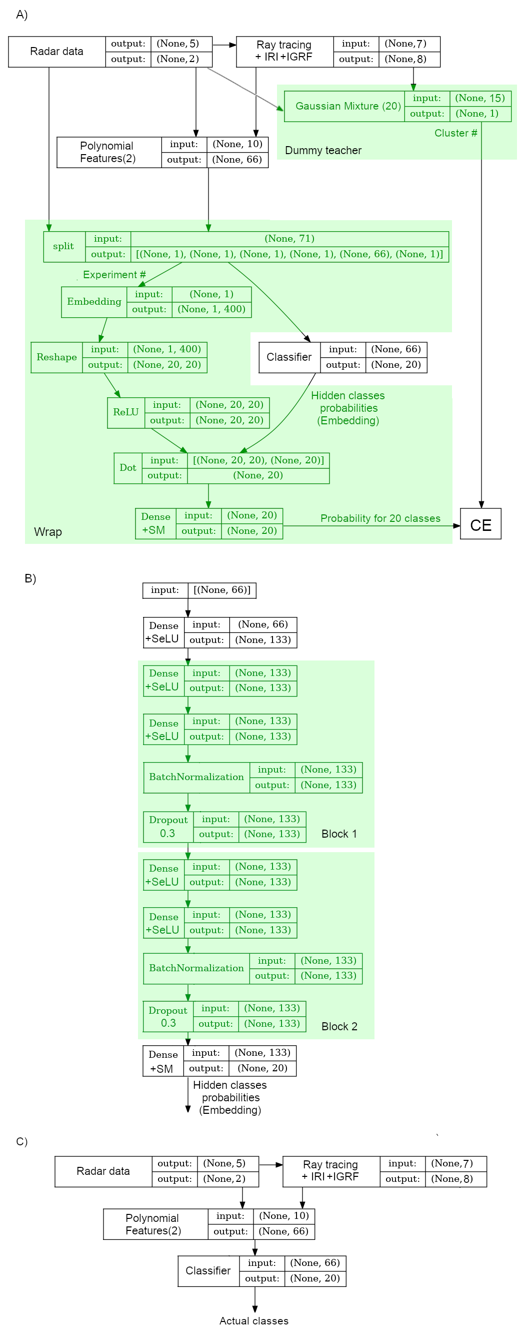
Figure 1: Architecture of the Wrapped Classifier with Dummy Teacher and dimensions of vectors. A) - network architecture in training mode; B) Classifier architecture C) - network architecture in processing mode. ”None” labels correspond to the number of records in the dataset.

From Fig.1A,C one can see that the network architecture is ideologically close to the word2vec network architecture, but instead of the embedding matrix for words, a neural network - Classifier is used (Fig.1B), and the problem of predicting word by its context is replaced by the problem of predicting Dummy Teacher cluster number by hidden classes probabilities. Classifier generates optimal embeddings and takes into account the physics of the problem by using only physically well-interpreted parameters for classification. This representation is further converted by the Wrap into classification closest to clusterization by Dummy Teacher. An important detail is that the numbering of the clusters differs from experiment to experiment, and the the clusters must be renumbered for each experiment. To do this, the Wrap uses adaptive embedding, which, unlike traditional vector-valued embeddings, is a non-negative matrix-valued embedding (implemented by sequential use of the Embedding, Reshape and ReLU layers of TensorFlow library). The experiment number is used as an index for the embedding (in our case, this is a unique number constructed from the radar number and the day number). The renumbering of classes is performed by matrix multiplication of the classes obtained from the Classifier by a matrix embedding that is unique for each experiment. Conceptually, this operation is close to a very simplified Attention [10] mechanism. The renumbered class obtained in this way goes to the decision layer. This method allows us to speed up the learning process and the memory amount required for the network training.

We use a polynomial straightening space (Polynomial Features, appends squares of parameters and all cross products of parameters) at the input of the Wrapped Classifier. This caused by to the fact that weighted sum of the squares of the Doppler shift and the signal spectral width is already used as a good criterion for the identification of groundscatter signals [3]. So taking into account the squares of the input features and the cross products of the input features, as will be shown below, increases the efficiency of the classification.

The Classifier is a fully connected network consisting of input and output layers, and hidden layers combined into two identical blocks: 2 fully connected layers + Normalization + 30% Dropout (shown in Fig.1B). All the activation functions, except for the output layer, are SeLU.

SeLU is used to reduce the effect of gradient fading, DropOut and Normalization - to reduce overtraining of the network and to speed up its training, respectively.

The number of neurons in each layer of the Classifier per one exceeds doubled dimension of the input data and is chosen in accordance with the Kolmogorov-Arnold theorem [11] for the most optimal representation of the input data. Classifier has about 83000 trained parameters, and Wrap has about 206000 trained parameters.

For training, the initial dataset (data from two radars for January-September 2021, ~ 3 million records) is splitted into training, validation and test datasets in proportion of 64%:16%:20%. The weighted cross-entropy is used as a loss function, the stop condition is the early stoping for 20 epochs based on the value of the AURPC metric on the validation dataset.

The difference from traditional schemes is that the embedding of the Classifier scheme is normalized - it is non-negative, and the sum of its components is equal to 1, which is implemented by Softmax output activation function. This allows interpreting the Classifier output as the probability of belonging the point to a particular (hidden) class.

The proposed algorithm consists of 3 stages:

1) adding to the experimental data obtained by the radar, the physical parameters calculated from these experimental data and physical models, making unlabeled dataset;

2) clustering each experiment of the resulting dataset by the Dummy Teacher to obtain a labeled training dataset for the Wrapped Classifier.

3) joint training of the Wrapped Classifier network (Wrap and Classifier) on labeled dataset to obtain an optimally trained Classifier from the condition of the maximum coincidence between the classification made by Wrapped Classifier and clustering made by the Dummy Teacher.

To speed up the network training each stage was carried out sequentially, with saving the resulting datasets to storage. To interpret the new data, only stage 1 is required, followed by the processing of the data received from 1st stage by the trained Classifier. Let us describe the stages in details.

2.1 Stage 1: adding physical parameters

Dummy Teacher separates the data according to all the dataset features available, not paying a special attention to the physicality of these parameters - their suitability for interpreting the physical mechanisms of formation of a particular type of scattered signal. Such a processing that is not based on physical mechanisms will be nearly useless later for the interpretation of the data. Therefore, the Classifier does its classification based only on well-understandable physical parameters included into the dataset, both measured and numerically simulated by physical models based on the parameters measured by the radar. This allows us later to interpret the classes obtained by the Classifier from a physical point of view.

The main parameters affecting the interpretation of the scattered signals in the ionosphere are the position of the scattering region on the radiowave propagation trajectory, the angle between the propagation trajectory and the Earth’s magnetic field at the scattering point, and the scattering height[2]. It is also important for consideration to take into account the hop-like nature of propagation to understand at which hop of the trajectory the scattering occurred, and how many times the radio signal was reflected from the ionosphere and from the Earth’s surface.

Therefore, based on the measured parameters of the received signal and known experimental setup, we can calculate additional physical parameters using radiophysical and geophysical models describing radiowave propagation in an inhomogeneous ionosphere.

Geometric optics (ray tracing) [12] was used to calculate the wave propagation trajectory in the approximation of non-magnetized ionosphere. Ionospheric refraction is calculated from the international reference model of the ionosphere IRI-2012[13]. The Earth’s magnetic field is calculated from the international reference magnetic field model IGRF [14]. As input parameters for calculating the trajectory, we used: the received signal elevation angle (it was assumed that it coincides with the emission elevation angle) calibrated by the method[15]; the azimuth of the radar beam; the operating frequency of the radar; the geographic position of the radar; date/time and radar range.

As the physical parameters characterizing the calculated propagation trajectory, the following parameters were chosen, obtained by raytracing:

- the sine of the angle between the wave vector of the radiowave and the horizon at the scattering point. It allows one to estimate how close the scattering point to the point of the reflection from the ionosphere, where this parameter becomes zero. Before the point of ionospheric reflection this parameter is greater than zero, and after the point of reflection (this parameter is less than zero. This allows to later interpret classes in terms 0.5 and 1.5 hop positions;

- the cosine of the angle between the wave vector and the Earth’s magnetic field at the scattering point. This parameter allows one to determine whether the scattering is near the perpendicular to the magnetic field (aspect sensitive scattering) or not. In case of scattering from magnetically oriented inhomogeneties the parameter is close to zero;

- the sine of the angle between the wave vector and the horizon in the middle of the path length to the scattering point. It allows one to understand whether the signal is scattering from the Earth’s surface, because in this case this parameter should be close to zero;

- the sine of the angle between the wave vector and the horizon at a quarter of the path length to the scattering point. As in previous case, it allows us to estimate whether the signal is the second scattering from the ground after two-hop propagation or not.

- the sine of the angle between the wave vector and the horizon at three quarters of path length to the scattering point. It has similar interpretation as the previous case.

- the hop number for hop propagation (the number of reflections from the Earth’s surface + 1). It allows one to additionally guess at which hop of the trajectory the scattering occurs.

- the altitude at which the scattering occurs. It allows one to guess about a possible mechanism of the scattering: the region of 70-100 km corresponds to meteor trail scattering, 100-130 km - scattering in the E-layer, above 150 km - scattering in the F-layer, if the altitude close to zero - most likely this is scattering from the Earth’s surface. The heights greater than F2 maximum height (about 400km) usually should not occure, so in this case propagation trajectory calculated incorrectly.

- the effective scattering height - the height obtained in the assumption of straight-line (refraction-free) wave propagation. This parameter can help to interpret the cases where refraction in the ionosphere can be neglected. For example, the case of meteor trail scattering and scattering in the E-layer at 0.5 hop. In most often cases the interpretation of this parameter depends on sounding frequency, so using of this parameter could cause questions, and will be discussed later.

In addition, the physical parameters characterizing the scattering mechanism are the Doppler shift of the radiowave (associated with the velocity of the scattering irregularities and propagation in non-stationary ionosphere) and the spectral width of the signal (associated with the lifetime of the scattering irregularities).

Thus, the classification model (Classifier) depends on 10 input parameters, only two of which (Doppler shift and spectral width) were directly measured by the radar, and the rest 8 of them were obtained using numerical simulation based on the measured parameters of received signal. These parameters are illustrated in Fig.2.

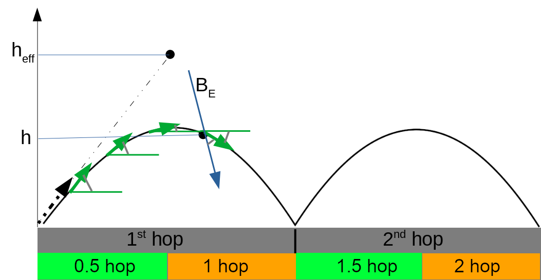
Figure 2: Scheme for calculating physical parameters determined from numerical simulations. The black solid line is the trajectory of the radio signal propagation, calculated using ray-tracing. blue arrow - the direction of Earth’s magnetic field, green horizontal lines marks the direction of the horizon, green solid arrows - the direction of propagation of the radio signal. The half hops marked at the bottom (0.5,1,1.5,2) are not used as parameters for the network, but are used later when interpreting the classes.

The propagation trajectory of the radiowave is calculated by the geometric optics method [12] based on the ionosphere model (given by the IRI model) and the characteristics of the radio wave (the frequency of the sounding signal and the angles of its arrival - azimuth and elevation). The necessary smoothness of the ionosphere in calculations is provided by fitting it with local B-splines of the 2nd order (parabolic interpolation of electron density between spatial and altitude points given by the IRI model). The radiowave is thought propagating in a plane determined by the sounding azimuth. The ionosphere is assumed to be two-dimensionally inhomogeneous (over the propagation direction and over the height).

2.2 Stage 2: Clustering by Dummy Teacher

In order to further train the classification algorithm based on the initially unlabeled data, within the framework of this algorithm, it is necessary to create a labeled training dataset. Sometimes, the labeling of the source dataset can be made manually, but it takes too much efforts to do this. In this paper we use another approach, developed for optimal embeddings in language models: search for the representation (hidden classes) optimal for solving a model problem by another network, and train two these networks together. As a model problem, the imitation of clustering by Dummy Teacher is used. Thus, the Dummy Teacher is not the main element of the network, but rather a supporting one, which allows, however, to optimally train Classifier network.

Scattered signals usually can be separated into a types according to the boundary conditions of some measured parameter: these can be short ranges for meteor trail scattering or low velocity and spectral width for a groundscatter [2]. Therefore, it looks reasonable to use for clustering the algorithms that finds an optimal limited areas occupied for points of a given class. We used for clustering the probabilistic model, describing the data as a superposition of 20 multidimensional Gaussian distributions with their own parameters. Each of gaussian describes its own cluster of points in multidimensional coordinates. This clustering algorithm is widely known as Gaussian mixture model.

The parameters that the Dummy Teacher will use, in addition to the physical parameters obtained as a result of simulation in stage 1, are the following experimental features: time (UT), spatial coordinates (beam number or azimuth, radar distance, elevation of the received signal) and the sounding frequency. For a more accurate separation during clustering, we use only signals with a high signal-to-noise ratio ($>3dB$). The power of the radio signal is not used in the algorithm due to the data contain various power variations that are not related to the type of signal: radio signal absorption in the D-layer and its focusing–defocusing due to the propagation of the radio wave in an inhomogeneous ionosphere [16].

Clustering of each experiment (the experiment number is a unique number composed of the day number and the radar number) is carried out independently, which allows us to speed up the clustering algorithm and put an additional uncertainty to the Dummy Teacher.

2.3 Stage 3: Training the Wrapped Classifier

Our main task is to build and train the Classifier network, which carries out the optimal classification of our data. The Classifier architecture is shown in Fig.1B.

As the input of this network the physical parameters are used, which we consider to be responsible for the signals identification, taking into account the physical mechanisms of the formation of signals of different types. This allows us to interpret the obtained classes in the future.

Typically, Doppler velocity and spectral width are used to identify groundscatter signals. In addition to them, the scattering height, which is responsible for the echo formation mechanism, carries useful information. In particular, at altitudes below 100 km, the main signal source is scattering by meteor trails; at altitudes up to 400 km this is scattering in the ionosphere, and the higher altitudes more likely corresponds to incorrect calculation of radiowave trajectory. The Classifier also uses parameters obtained during numerical simulation: key parameters characterizing the propagation trajectory, the aspect angle with the Earth’s magnetic field at the scattering point, the real scattering height, and so on.

It should be noted that the parameters used by the Dummy Teacher and by the Classifier are different. The Classifier uses only physical parameters that do not depend on the operating mode of the radar, with which the optimal classification should be associated: scattering height, trajectory angle with the magnetic field in the scattering region, trajectory behavior features, propagation hop number, Doppler frequency shift and signal spectral width. Dummy Teacher uses, in addition to the physical parameters, also characteristics related to the time and operating mode of the radar: the universal time, radar beam number, ray elevation, radar range and sounding frequency.

Thus, the Classifier network make an extraction of meaning from the input data and produces a vector (embedding) characterizing the classification of signals from physical point of view, into hidden classes optimal to predict Dummy Teacher clustering. In order to this embedding has an interpretable probability meaning, it is normalized: the sum of all coordinates of the vector is 1, and all the coordinates are non-negative. This is implemented using the standard machine learning approach - softmax activation function at the output of the Classifier. This allows us to interpret this embedding as the probability that the input point belongs to one or another ”hidden” class. This embedding will be used later by the ”Wrap” network to produce prediction of Dummy Teacher cluster number. The dimension of this embedding vector is fixed and set to 20 in order to exceed the possible number of significant types in the received signal. As a result of training this dimension will be decreased automatically (some of embedding coordinates will be nearly zero), as it will be shown later.

The schema is trained based on the best fit by the Wrapped Classifier the clusterization of the Dummy Teacher and algorithmically formulated as classification training, where labels come from Dummy Teacher and their predictions come from Wrapped Classifier.

The architecture of the network is shown in Fig.1A. Such an architecture allows training the Wrapped Classifier to classification optimal from the point of view of predicting the results of a Dummy Teacher. This architecture automatically renumerates the cluster numbers for each experiment independently. When processing new data, we do not need to use Wrap, but use only Classifier network and its output (hidden classes probabilities) as physics-based classification of the signals. So after training Wrapped Classifier the Wrap can be thrown away.

During training, weighted cross-entropy is used as a loss function, where the weights are the inverse frequency of a cluster number in the training dataset. This allows to automatically balance the dataset, and thereby to improve fitting quality.

AURPC is used as a metric of the prediction quality, because it works correct enough in a case of a possible class imbalance. When training, we use a early stopping over 20 epochs, when maximum AURPC is found at validation dataset, as an overtrain stopping criterion. Gradient descent method is used with ADAM optimizer, with batch size 32. Full dataset size is about 3 million records, split into training, validation and test datasets is made as 64%:16%:20%. The propagation parameters are calculated in the C language using the IRI-2012 and IGRF models, implemented in the Fortran language. Network training is implemented in Python, Dummy Teacher is implemented using sklearn library functions, Wrapped Classifier is implemented using TensorFlow/Keras library functions. The AURPC value achieved as a result of training was 0.659 after 173 training epochs, which looks as a sufficient result for a 20-class classification.

3 Results and their interpretation

3.1 Training results

Fig.3 shows the result of classifying the 03/08/2021 data obtained by EKB and MAGW radars by the trained Classifier algorithm into 20 classes (c0-c19). The data from all radar beams are displayed simultaneously. The figure shows a reasonable separation of the data into classes. Meteor scatter (class 14) is one of the most easily interpreted classes, corresponding to scatter at radar ranges up to 450 km [15].

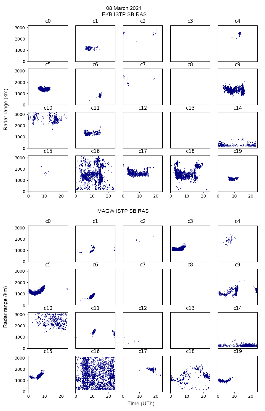
Figure 3: Points positions of hidden classes of the Classifier as a function of radar range and time. Data from EKB and MAGW ISTP SB RAS radars during 08/03/2021.

3.2 Interpreting the classes

To interpret all the classes, the mean value and standard deviation of each of the 10 Classifier input parameters and radar distance are calculated for each class over whole available dataset (January-September 2021). According to the average values and standard deviations of these parameters, the interpretation of each class is carried out. In addition the degree of interpretability of the classes is calculated - the number of points in which the mean height of their classes does not exceed the physically expected value of 400 km - the maximum of the F2 layer height. Higher values indicate inaccurate ionospheric model or inaccurate received signal elevation angle measurements, which leads to errors in calculating the wave propagation trajectory. The part of data that cannot be interpreted from this point of view is 22%, and there are 78% of interpretable data points.

Classes 0,2,7,10,17,18 due to the high model scattering height exceeding the height of the ionospheric maximum were assigned by us to the classes with poorly calculated propagation trajectory. Scattering at high altitudes most likely does not correspond to reality because of the low background electron density at these altitudes, which leads to a low probability of intense irregularities at altitudes above F2 maximum. Therefore, most likely, this signal is scattered at lower altitudes, so the ray-tracing trajectory calculations are most likely incorrect. This is associated with known problems of the accuracy of ionospheric models[17], and with the inaccuracy of measuring the elevation angle of the radio wave arrival[15].

Class 8 is empty, and classes 2, 4, and 13 are relatively rare, so they should not be taken into account.

Classes 1,11 are localized at ranges of 800-1500 km, at heights of 35-200 km, non-aspect sensitive (the average angle with the magnetic field is far from perpendicular), on the descending part of the propagation trajectory. Therefore they can be interpreted as long-range (1hop, after reflection from ionosphere) meteor scattering or as a groundscatter.

Class 3 - rarely observed by the EKB radar, but frequently observed by the MAGW radar, non-aspect sensitive, at heights of 50-110 km, at ranges of 1000-1250 km, after reflection from the ground on the ascending part of the trajectory. It can be interpreted as 1.5hop meteor scatter.

Class 5 - non-aspect sensitive scattering at altitudes of 20-110 km, after reflection from the ground, on the ascending part of the trajectory. It can be interpreted as a groundscatter.

Class 6 - aspect sensitive scattering from distances of 500-800 km, at heights of 160-260 km on the ascending part of the trajectory. It can be interpreted as 0.5E or 0.5F scatter.

Class 9 - non-aspect sensitive scattering at ranges 600-1600 km, at altitudes 40-180 km, on the descending part of the trajectory. It can be interpreted as a groundscatter.

Class 12 - aspect sensitive scattering at altitudes of 200-300 km and ranges of 380-700 km, on the ascending part of the trajectory. It can be interpreted as 0.5F scatter.

Class 14 is scattering at heights of 50-130 km, at distances of 180-470 km, on the ascending part of the trajectory. It can be interpreted as a 0.5 hop meteor trail echo.

Class 15 - aspect sensitive scattering at heights of 125-190 km, 1100-1650 km, after reflection from the ground, on the ascending part of the trajectory, can be interpreted as 1.5F scatter.

Class 16 - aspect sensitive scatter at heights of 0-550 km, at distances 500-2000 km, partially before, partially after reflection from the ground. As one can see from Fig.3 it can be interpreted as an indefinite class, consistent from points difficult to identify. This class will not be taken into account.

Class 19 - non-aspect sensitive scattering at altitudes of 10-120 km, on the descending part of the trajectory, at ranges of 1000-1200 km, can be interpreted as groundscatter.

Thus, the scattered signal can be divided into 11 interpretable classes, and 9 classes should not be taken into account. An example of observations labeled in accordance with this classification is shown in the Fig.4. The figure shows only the signals from interpreted classes.

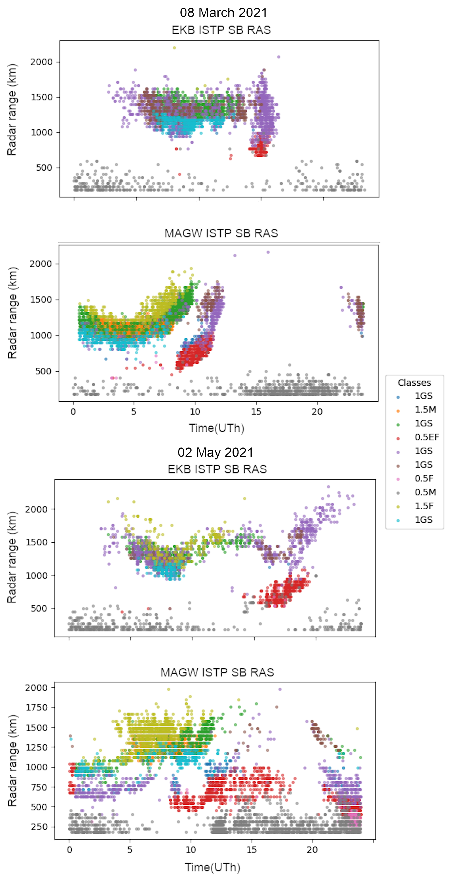
Figure 4: An example of automatic classification of radar data EKB ISTP SB RAS and MAGW ISTP SB RAS for 08 March 2021 (top) and 02 May 2021 (bottom)

3.3 Simplifying the network

To investigate the possibilities of simplifying the Wrapped Classifier network, its simplified variants were analyzed: removing the straightening space (PF) before Wrapped Classifier, removing one of the blocks (B2) from the Classifier, removing the dependence on the refraction-free scattering height ($h_{eff}$). As an additional information, the ability of the algorithm to separate meteor trail scattering into a separate class on both radars was estimated (this is determined from the average physical parameters of the class - the signals of this class should have an average altitude of 70-100 km and an average radar range not exceeding 400 km). The analysis results are summarized in the table 1.

Table 1: Comparison of results for simplified network variants. PF - Polynomial features transformation is included into Wrap, B2 - Block 2 included into Classifier, $h_{eff}$ - refraction free scattering height is used as input parameter. Interpretable - percent of points in classes with correct scattering height. ME - meteor trail echo.

PF	B2	$h_{eff}$	AURPC	Interpretable	ME class exists?
yes	yes	yes	0.659	78%	yes
yes	yes	no	0.593	77%	no
yes	no	yes	0.627	85%	no
yes	no	no	0.575	89%	no
no	yes	yes	0.550	77%	no
no	yes	no	0.522	74%	no
no	no	yes	0.605	86%	no
no	no	no	0.556	78%	no

As can be seen from the results, the presented version of the Wrapped Classifier network provides the best AURPC value, a good percentage of class interpretability, and is the only variant that provides the detection of meteor trail scattering by both radars. Thus, it looks like no simplification of the network architecture is necessary.

4 Conclusion

In the paper a method for automatic classification of signals received on EKB and MAGW ISTP SB RAS radars during January-September 2021 is described. The method is suitable for automatic physical interpretation of the experimental data classification in realtime. We called this algorithm Wrapped Classifier with Dummy Teacher. During training, it classifies the radar data to 20 hidden classes, used for optimal prediction the data clustering by Dummy Teacher (the probabilistic method of dividing data on 20 clusters with different gaussian distributions).

We extended parameters obtained by the radar with additional parameters, calculated during numerical simulation of radiowave propagation using ray-tracing technique and IRI-2012 and IGRF models for ionosphere and Earth’s magnetic field correspondingly. For clustering by Dummy Teacher algorithm we use the whole dataset of available parameters (measured and simulated ones). For classification by Wrapped Classifier algorithm it uses only well physically interpreted parameters. As a result we found 11 well-intepretable classes from a physical point of view in the available data.

Necessary for this method is a high-quality elevation calibration of the radars and high-accuracy ionospheric model. They are necessary for correct calculations of the signal propagation trajectory. For simulation we use the model ionosphere (IRI-2012) and ray-tracing calculation of beam propagation in the ionosphere. Errors associated with this lead to the appearance of classes that cannot be interpreted from the point of view of radio wave propagation. They are characterized by a large expected scattering height, above the maximum of the F2 layer. The number of such uninterpretable datapoints is about 22%.

References

- [1] S. Yu and J. Ma, “Deep Learning for Geophysics: Current and Future Trends,” Reviews of Geophysics, vol. 59, no. 3, p. e2021RG000742, 2021.
- [2] N. Nishitani, J. Ruohoniemi, M. Lester, J. B. H. Baker, A. Koustov, S. Shepherd, G. Chisham, T. Hori, E. G. Thomas, R. Makarevich, A. Marchaudon, P. Ponomarenko, J. A. Wild, S. Milan, W. A. Bristow, J. Devlin, E. Miller, R. A. Greenwald, T. Ogawa, and T. Kikuchi, “Review of the accomplishments of mid-latitude Super Dual Auroral Radar Network (SuperDARN) HF radars,” Progress in Earth and Planetary Science, vol. 6, no. 1, p. 27, Mar 2019.
- [3] G. Blanchard, S. Sundeen, and K. Baker, “Probabilistic identification of high-frequency radar backscatter from the ground and ionosphere based on spectral characteristics,” Radio Science, vol. 44, no. 5, p. RS5012, 2009.
- [4] A. Ribeiro, J. Ruohoniemi, J. Baker, S. Clausen, S. de Larquier, and R. Greenwald, “A new approach for identifying ionospheric backscatter in midlatitude SuperDARN HF radar observations,” Radio Sci., vol. 46, p. RS4011, 2011.
- [5] I. A. Lavygin, O. I. Berngardt, V. P. Lebedev, and K. V. Grkovich, “Identifying ground scatter and ionospheric scatter signals by using their fine structure at ekaterinburg decametre coherent radar,” IET Radar, Sonar & Navigation, vol. 14, no. 1, pp. 167–176, 2020.
- [6] O. Berngardt, N. Zolotukhina, and A. Oinats, “Observations of field-aligned ionospheric irregularities during quiet and disturbed conditions with EKB radar: First results,” Earth, Planets and Space, vol. 67, p. 143, 2015.
- [7] D. Jurafsky and J. Martin, Speech and Language Processing: An Introduction to Natural Language Processing, Computational Linguistics, and Speech Recognition, ser. Prentice Hall series in artificial intelligence. Pearson Prentice Hall, 2009.
- [8] T. Mikolov, K. Chen, G. Corrado, and J. Dean, “Efficient Estimation of Word Representations in Vector Space,” arXiv e-prints, p. arXiv:1301.3781, Jan. 2013.
- [9] I. Sutskever, O. Vinyals, and Q. V. Le, “Sequence to Sequence Learning with Neural Networks,” arXiv e-prints, p. arXiv:1409.3215, Sep. 2014.
- [10] A. Vaswani, N. Shazeer, N. Parmar, J. Uszkoreit, L. Jones, A. N. Gomez, L. Kaiser, and I. Polosukhin, “Attention Is All You Need,” arXiv e-prints, p. arXiv:1706.03762, Jun. 2017.
- [11] V. Arnold, “On the function of three variables,” Amer. Math. Soc. Transl., pp. 51–54, 1963.
- [12] V. Ginzburg, The Propagation of Electromagnetic Waves in Plasmas, ser. Commonwealth and International Library. Pergamon Press, 1970.
- [13] Bilitza, Dieter, Altadill, David, Zhang, Yongliang, Mertens, Chris, Truhlik, Vladimir, Richards, Phil, McKinnell, Lee-Anne, and Reinisch, Bodo, “The international reference ionosphere 2012 - a model of international collaboration,” J. Space Weather Space Clim., vol. 4, p. A07, 2014.
- [14] E. Thébault, C. C. Finlay, C. D. Beggan, P. Alken, J. Aubert, O. Barrois, F. Bertrand, T. Bondar, A. Boness, L. Brocco, E. Canet, A. Chambodut, A. Chulliat, P. Coïsson, F. Civet, A. Du, A. Fournier, I. Fratter, N. Gillet, B. Hamilton, M. Hamoudi, G. Hulot, T. Jager, M. Korte, W. Kuang, X. Lalanne, B. Langlais, J.-M. Léger, V. Lesur, F. J. Lowes, S. Macmillan, M. Mandea, C. Manoj, S. Maus, N. Olsen, V. Petrov, V. Ridley, M. Rother, T. J. Sabaka, D. Saturnino, R. Schachtschneider, O. Sirol, A. Tangborn, A. Thomson, L. Tøffner-Clausen, P. Vigneron, I. Wardinski, and T. Zvereva, “International Geomagnetic Reference Field: the 12th generation,” Earth, Planets and Space, vol. 67, no. 1, p. 79, 2015.
- [15] O. I. Berngardt, R. R. Fedorov, P. Ponomarenko, and K. V. Grkovich, “Interferometric calibration and the first elevation observations at EKB ISTP SB RAS radar at 10-12 MHz,” Polar Science, p. 100628, 2020.
- [16] O. I. Berngardt, J. P. St. Maurice, J. M. Ruohoniemi, and A. Marchaudon, “Seasonal and diurnal dynamics of radio noise for 8-20MHz poleward-oriented mid-latitude radars,” arXiv e-prints, p. arXiv:2107.11532, Jul. 2021.
- [17] Z. Liu, H. Fang, L. Weng, S. Wang, J. Niu, and X. Meng, “A comparison of ionosonde measured foF2 and IRI-2016 predictions over China,” Advances in Space Research, vol. 63, no. 6, pp. 1926–1936, mar 2019.