supplemental
A generalized likelihood based Bayesian approach for scalable joint regression and covariance selection in high dimensions
Abstract
The paper addresses joint sparsity selection in the regression coefficient matrix and the error precision (inverse covariance) matrix for high-dimensional multivariate regression models in the Bayesian paradigm. The selected sparsity patterns are crucial to help understand the network of relationships between the predictor and response variables, as well as the conditional relationships among the latter. While Bayesian methods have the advantage of providing natural uncertainty quantification through posterior inclusion probabilities and credible intervals, current Bayesian approaches either restrict to specific sub-classes of sparsity patterns and/or are not scalable to settings with hundreds of responses and predictors. Bayesian approaches which only focus on estimating the posterior mode are scalable, but do not generate samples from the posterior distribution for uncertainty quantification. Using a bi-convex regression based generalized likelihood and spike-and-slab priors, we develop an algorithm called Joint Regression Network Selector (JRNS) for joint regression and covariance selection which (a) can accommodate general sparsity patterns, (b) provides posterior samples for uncertainty quantification, and (c) is scalable and orders of magnitude faster than the state-of-the-art Bayesian approaches providing uncertainty quantification. We demonstrate the statistical and computational efficacy of the proposed approach on synthetic data and through the analysis of selected cancer data sets. We also establish high-dimensional posterior consistency for one of the developed algorithms.
1 Introduction
We consider joint variable and precision matrix selection in high-dimensional multivariate regression models with multiple responses. In particular, we consider two sets of variables: the matrix whose rows comprise of samples on predictor variables and the matrix whose rows comprise of matched samples (same set of entities) on response variables. We are interested in inferring a graphical model on the variables from the data, while accounting for the effect of the data. The corresponding multivariate regression model is given by
| (1) |
where is an matrix whose rows comprise of the noise vectors and is a matrix of regression coefficients. To make things concrete, assume that are independent, and
This is equivalent to assuming that the noise vectors are i.i.d. . The matrix captures the dependence between the response variables conditional on the predictor variables, and the matrix captures the effect of the predictor variables on the response variables.
For example, in molecular biology applications, multiple Omics modalities are profiled on the same set of samples. Then, following the central dogma of biology, the predictor variables could correspond to the DNA level (e.g., copy number or methylation data), while the response variables to the transcriptomic level (mRNA expression). Another possibility is that the predictors correspond to the transcriptomic level and the responses to the proteomic level. Thus, the regression coefficients in encode transcriptional or translational dependencies, while the entries of reflect statistical associations within a molecular compartment.
We focus on the problem under a high-dimensional setting, wherein and/or is larger than or comparable to the sample size . In such sample starved settings, imposing sparsity in and offers a simple and effective approach for reducing the effective number of parameters. The sparsity patterns in and often have specific scientific interpretations and can help researchers understand the underlying relationships between variables in the data set. To summarize, our goal is simultaneous sparse estimation of and , and the use of estimated sparsity patterns to understand relevant dependence structures.
The above problem has been studied in the literature. On the frequentist side, various penalized likelihood based methods have been proposed. Many of these methods use an penalty that encourages sparsity both in and . Various optimization algorithms have been employed; see Friedman et al. (2008), Rothman et al. (2010), Lee and Liu (2012), Cai et al. (2013), Lin et al. (2016a) and references therein. Note that the conditional log-likelihood for response given can be written as
| (2) |
and is not jointly convex in and . Hence, many popular algorithms (e.g., block coordinate descent) for optimizing a penalized version of this log-likelihood may fail to converge to the global optimum, especially in settings where , as pointed out in Lee and Liu (2012). However, the log-likelihood is bi-convex, i.e., it is convex in for fixed and in for fixed . The bi-convexity is leveraged in Lin et al. (2016a) to develop a two-block coordinate descent algorithm which converges to a stationary point of the objective function assuming that all iterates need to be within a ball of certain radius (a function of the model dimensions and the sample size ) that in addition contains the true data generating parameters. This condition is then shown to hold with high probability.
Some recent papers such as Sohn and Kim (2012), Yuan and Zhang (2014), McCarter and Kim (2014) consider an alternate parameterization where . The likelihood can be shown to be jointly convex in , and the respective algorithms in these papers provide sparse estimates of and by using appropriate penalties. However, sparsity in does not in general correspond to sparsity in . In many applications, the linear model with the parameterization is the natural modeling tool, and sparsity in the regression coefficient matrix has a specific scientific interpretation. This interpretability may be lost if sparsity is instead imposed on . See (Lin et al., 2016a, Section 5) for a detailed discussion.
Bayesian methods offer a natural framework for addressing uncertainty quantification of model parameters through the posterior distribution, and several Bayesian approaches have also been proposed in the literature. Brown et al. (1998) propose a Bayesian approach for the joint estimation of and , but restrict the sparsity pattern in to be such that each row of is completely sparse or completely dense. Richardson et al. (2010) allow for a general sparsity pattern in , but restrict to be a diagonal matrix. Bhadra and Mallick (2013) use spike-and-slab prior distributions to induce sparsity in (conditional on ), and -Wishart prior distributions coupled with independent Bernoulli priors on the sparsity pattern in . Similar to Brown et al. (1998), they restrict the rows of to be completely sparse or completely dense, and also restrict the sparsity pattern in to correspond to a decomposable graph. In a related work Consonni et al. (2017), the authors develop an objective Bayesian approach for Directed Acyclic Graph estimation in the presence of covariates. This approach induces sparsity in the Cholesky factor of and corresponds to directly inducing sparsity in , when the underlying sparsity pattern is decomposable. In a recent work, Deshpande et al. (2019) propose a scalable Bayesian approach using spike-and-slab Laplace prior distributions to induce sparsity in and . The work employs an Expectation Conditional Maximization algorithm to find the (sparse) posterior mode, and thereby obtain sparse estimates of and . However, methods to generate samples from the posterior distribution are not explored, and hence uncertainty quantification in the form of posterior credible regions/intervals is not available. In Li et al. (2021) the authors propose a Gaussian likelihood based fully Bayesian procedure for the simultaneous estimation of the mean vector and the inverse covariance matrix which provides measures of uncertainty. However, in moderate/high dimensional settings it might run into scalability issues as pointed out in Section 4.
Note that in most of the above cited literature, and in this paper, two layers of variables are considered. The matrix captures the effect of the top layer (predictors) on the bottom layer (responses), while the matrix captures the conditional covariance structure of the bottom layer. It is possible to consider a scenario where we have a chain of multiple layers of variables, each layer affecting the layer below it (see the setting in Lin et al. (2016b)), thereby giving rise to multiple pairs of and matrices. Due to the factorization of the likelihood based on the Markov property induced by the chain structure, any method developed for the two-layer setting can be extended in a reasonably straightforward way to the multiple layer setting, subject to some model parameter identifiability restrictions (see Section 3.4 in Lin et al. (2016b)).
In Ha et al. (2020b), the authors consider the multiple layer setting, and develop a generalized likelihood based Bayesian approach for simultaneous sparse estimation of the and pair. In Peng et al. (2009a) and Khare et al. (2015), the use of a regression based generalized likelihood has been shown to significantly improve the computational efficiency compared to Gaussian likelihood based methods for standard graphical models (no presence of predictors). In Ha et al. (2020b) sparsity inducing spike-and-slab prior distributions are used for the entries of and , and an MCMC algorithm (called BANS) based on add/delete/swap moves in the space of sparsity patterns is developed to generate approximate samples from the posterior distribution. In simulation experiments, scenarios with up to ten layers of variables, and up to 20 variables in each layers are considered. However, the algorithm starts to run into serious computational issues when the number of variables in each layer is bumped up to 200 (with two layers). One reason for this is the need for several matrix inversions to compute Metropolis-Hastings based rejection probabilities in each iteration of the BANS algorithm (see Sections 2.2 and 4 for more details). A faster algorithm called BANS-parallel, wherein computations corresponding to each response variable can be parallelized, has also been developed in Ha et al. (2020b). However, this approach ignores the symmetry in which negatively affects the quality of the estimates, and again requires matrix inversions for various Metropolis-Hastings steps (see Remark Remark at the end of Section 2). In short, existing Bayesian approaches suffer from at least one of the following drawbacks: (i) restrict to a subclass of sparsity patterns; (ii) focus on estimating the posterior mode and not on sampling from the posterior distribution; (iii) are not computationally scalable due to excessive use of matrix inversions.
The goal of this paper is to develop a computationally scalable generalized likelihood based Bayesian procedure for joint regression and precision matrix selection, which can account for arbitrary sparsity patterns in and , and provide uncertainty quantification. First, we leverage ideas in Khare et al. (2015) for standard graphical models (no predictors) to the current setting, and construct a regression based generalized likelihood that is bi-convex in and . The generalized likelihood in Ha et al. (2020b), which corresponds to the predictor adjusted version of the generalized likelihood in Peng et al. (2009a), is neither jointly convex, nor bi-convex. In the standard graphical model setting, it has been demonstrated in Khare et al. (2015) that convexity plays an important role in improved algorithmic and empirical performance of the generalized likelihood as compared to the one in Peng et al. (2009a). Next, we develop a Gibbs sampling algorithm (referred to as the joint algorithm) to sample from the corresponding posterior (using spike-and-slab priors for entries of and ). With entry-wise updates of and involving standard distributions, we completely avoid the matrix inversions needed for the Metropolis-Hastings steps in BANS and the resulting algorithm is significantly computationally faster. As an illustrative example, with responses and predictors, the proposed MCMC algorithm, coded in R/Rcpp, completes 3000 iterations (each iteration cycles through all the entries of and ) in less than 5 minutes. In the same setting, BANS (implemented using R/Rcpp code available on Github) was only able to finish less than 100 iterations in 4 days.
Several frequentist methods in the literature, such as those in Lee and Liu (2012) and Cai et al. (2013), consider a step-wise approach for sparse estimation of and . In this approach, regressions corresponding to each of the responses are used to obtain sparse estimates of columns of . The resulting estimate of is used to compute plug-in covariate adjusted responses, subsequently provided to a standard graphical model estimation procedure to obtain a sparse estimate of . As a Bayesian analog of this approach, and for faster computation, we develop a step-wise algorithm for joint regression/covariance selection. In this approach, we first focus on estimation/selection for by treating as a diagonal matrix and combining the resulting Gaussian likelihood with spike-and-slab priors on entries of . An appropriate posterior estimate of is then used to compute covariate-adjusted responses (or pseudo-errors) . In the second step of the algorithm, the generalized likelihood of Khare et al. (2015), along with spike-and-slab priors on the entries of is used for selecting the sparsity pattern in . The computational advantage obtained by ignoring the cross-correlation in the responses for the estimation step clearly comes with the cost of some loss of statistical efficiency. However, we rigorously establish high-dimensional posterior model selection and estimation consistency of the resulting estimates in Section 3.1. As expected, the simulation experiments in Section 4 in general demonstrate a loss in statistical accuracy and roughly two times improvement in computational performance as compared to the joint algorithm.
The remainder of the paper is organized as follows. The joint and the step-wise algorithms are developed in Sections 2 and 3, respectively. High-dimensional posterior consistency results for the step-wise algorithm are provided in Section 3.1. An extensive simulation study evaluating the empirical performance of the proposed algorithms is presented in Section 4 and an analysis of a cancer data set is presented in Section 5. Proofs of the technical results along with additional simulation details are provided in a Supplementary document.
2 Joint sparsity selection for and using a bi-convex generalized likelihood
We develop a generalized likelihood based Bayesian approach for jointly estimating the sparsity patterns in and . Consider the log-likelihood denoted by in (2). One reason why block updates corresponding to optimization/MCMC algorithms for the corresponding penalized objective functions/posteriors run into computational issues, even in moderate dimensional settings, is the presence of the term, which leads to expensive matrix inverse computations. Let denote the column of the data matrix . Hence, is the collection of all the observations corresponding to the response. Then, the conditional density of given all the other responses (and of course, conditional on ) is given by
| (3) |
where and denote the columns of and respectively, and . The above follows by noting that when regressing the variable against the other variables, the regression coefficient of the variable is given by . Using ideas in Besag (1975), a generalized likelihood for can be defined by taking the product of these conditional densities. This is the regression based generalized likelihood used for the BANS algorithm in Ha et al. (2020b), and its form is given by
| (4) |
Taking logarithm of the expression in (4), shows that the problematic term in the log-Gaussian likelihood (2) is now replaced by a much simpler term in the generalized log-likelihood. However, the bi-convexity is lost, i.e., given , the function is not convex in . In the simpler setting of Gaussian graphical models with no predictors (i.e., no ), it was shown in Khare et al. (2015) that this lack of convexity can lead to severe convergence issues (in a penalized optimization context) and a convex version of the generalized likelihood was constructed. We adapt this idea in the more general setting of joint regression and precision matrix estimation in a Bayesian context.
In particular, by ‘weighting’ each observation with for the expression in (2), i.e., using the conditional density of , and then taking the product over every , we get the generalized likelihood
| (5) |
Next, we discuss some important features related to and its use for Bayesian inference.
-
•
The exponent in now becomes a quadratic form in , and the power of is now instead of (as compared to ). Hence, is bi-convex (convex in given , convex in given ) and in general analytically more tractable than .
-
•
Note that our primary goal, as far as is concerned, is sparsity selection. Hence, following Meinshausen and Bühlmann (2006), Peng et al. (2009a), Khare et al. (2015), we relax the constraint of positive definiteness for to the simpler constraint of just having positive diagonal entries. This relaxation leads to significant improvement in computational scalability. If a positive definite estimate of is needed for a downstream application, it can be obtained by a quick refitting step restricting to the selected sparsity pattern. The same relaxation of the positive definiteness constraint is also used for the BANS algorithm in Ha et al. (2020b). Such a relaxation is not possible for the Gaussian likelihood because of the presence of the term.
-
•
Although a generalized likelihood is not a probability density anymore, it can still be regarded as a data based weight function, and as long as the product of the generalized likelihood and the specified prior density is integrable over the parameter space, one can construct a posterior distribution and carry out Bayesian inference (see Bissiri et al. (2016); Alquier (2020) and the references therein).
To induce sparsity, we use spike-and-slab prior distributions (mixture of point mass at zero and a normal density) for the entries of and the off-diagonal entries of , and exponential priors for the diagonal entries of . Specifically, for and , we use the following priors:
where ’s and ’s are independently distributed and denotes the distribution with its entire mass at 0. Further, the hyperparameters denote the respective mixing probabilities for entries of and , and the hyperparameters are the respective prior slab variances.
The resulting generalized posterior distribution
is
intractable in the sense that closed form computation or direct sampling
is not feasible. However, straightforward calculations show that:
-
•
the full conditional posterior distribution of each entry of (given all the other parameters and the data) is a mixture of a point mass at zero and an appropriate normal density. For
where
-
•
the full conditional posterior distribution of each off-diagonal entry of (given all the other parameters and the data) is a mixture of a point mass at zero and an appropriate normal density. For
(6) where
-
•
The full conditional posterior density of each diagonal entry of (given all the other parameters and the data) is given as
(7) where
This is an univariate density with the unique mode at
where .
These properties allow us to construct a Metropolis-within-Gibbs sampler, which we call the Joint Regression Network Selector (JRNS), to sample from the joint generalized posterior density of and . One iteration of JRNS, given the current value of is described in Algorithm 1 below. Essentially, all entries of and off-diagonal entries of are sampled from the respective full conditional distribution. A Metropolis-Hastings approach is used for the diagonal entries of . In particular, a proposal is generated from a normal density centered at the conditional posterior mode for . The proposed value is accepted or rejected based on the relevant Metropolis based acceptance probability computed using the proposal normal density and the full conditional of . A more detailed description of this algorithm is presented in Section 9 of the Supplement.
2.1 Sparsity selection and estimation using MCMC output
The output from JRNS for an appropriate number of iterations (after the burn-in period), can be used as follows to estimate the sparsity patterns in the corresponding parameters. We follow the majority voting approach to construct such an estimate, wherein we include only those variables whose generalized posterior based marginal inclusion probabilities are at least (Barbieri and Berger (2004)). Let represent the sparsity indicator of for and . Then, represents the sparsity pattern in . For each let which is approximated by
| (8) |
The quantity in (8) is the proportion of iterations for which out of the iterations. If , the -th entry is considered non-zero in the estimated sparsity pattern of . It is to be noted that by Ergodic theorem the MCMC approximation given above in (8) converges to the generalized posterior probability, of being non-zero as . For large values of , it is very close to . Then, an estimate of is approximately obtained as
A similar majority voting approach based on the generalized posterior based marginal inclusion probabilities can be used to estimate the sparsity pattern in . In particular, if represents the sparsity indicator for for , then an estimate of is approximately obtained as
Further, an estimate of the magnitudes of the selected non-zero entries of can also be obtained as follows. If , then
An estimate of the magnitudes of the selected non-zero entries of can also be obtained similarly. As stated earlier, the positive definiteness constraint on is relaxed for faster sparsity selection. An examination of the output of JRNS for many of our simulation settings in Section 4 consistently revealed positive definite iterates. However, there is no general guarantee that these iterates or the resulting estimate of will be positive definite.
If one wants to enforce positive definiteness, it can be achieved through a post-processing step (see Lee et al. (2020)) which focuses on the induced posterior of , where
for some suitably chosen .
Note that is guaranteed to be positive definite and has the exact same off-diagonal entries as . Hence, if are the components of the iterates produced by the JRNS or step-wise algorithm, sparsity selection, inclusion probabilities and credible intervals for the off-diagonal entries are unchanged if one uses instead of . The transformation to only affects estimation of the diagonal entries . This additional eigenvalue check for computing takes computations and hence does not change the computational complexity of JRNS (see (10) below), and marginally increases the wall-clock time (less than 5% in all our simulation settings).
Another approach to ensure positive definiteness is to use the refitting idea from the penalized sparsity selection literature (see for example Ma and Michailidis (2016)). The estimators generated from penalized sparsity selection methods often suffer from (magnitude) bias issues, and one way to fix this is to obtain a constrained MLE of the desired parameter (by restricting to the the estimated sparsity pattern). Using this idea in our context, we compute the estimated sparsity pattern in and the regression coefficient matrix estimator from the MCMC output as described above. Now, we use the pseudo-errors (rows of ) as approximate samples from a distribution, and use the glasso function in R to compute the constrained MLE of restricted to the sparsity pattern .
Hyperparameter selection: Selecting hyperparameters is an important issue in any Bayesian approach. In sample-starved settings discussed in this paper, the choice of hyperparameters may have a significant impact on the resulting estimates (see the Supplementary section 10.2 for more illustrations or details). A standard approach to choose the hyperparameters will be to use cross validation wherein we consider a grid of values for the hyperparameters and select the set of values based on the minimum prediction error. However, this method can be computationally expensive. If one does not have the computational resources or time to carry out the cross validation technique, another approach is to make some sensible objective choices as discussed below.
For JRNS, we have the prior mixture probabilities , the prior slab variances and and as hyperparameters. For and one can always consider a flat prior in which case we will get a beta-update for and in every iteration of the Gibbs sampler. Another choice of and which is motivated by the theoretical results in this paper and also in Cao et al. (2019), Narisetty and He (2014) is to take and . We use these choices in the simulation studies and obtain good results. For and one may choose values around 1 or for a more principled choice one may choose objective Inverse-Gamma priors with shape = and rate = as suggested in Wang (2012). These will result in straightforward Inverse-Gamma updates for and in each iteration. One may consider the Gamma prior with the same shape and rate values for as well.
2.2 JRNS and BANS: A computational cost comparison
Next, we discuss the computational cost associated with the proposed JRNS algorithm, and compare it with the computational cost for the BANS algorithm in Ha et al. (2020b). The structural differences in the generalized likelihoods used by the two algorithms have been described in the discussion surrounding equations (4) and (5). As we describe below, there are also crucial differences between the two approaches at the computational level that lead to a significant difference in overall computational costs.
-
•
Algorithm 2, as described in Section C of the supplementary document, provides the detailed pseudo-code for one iteration of the JRNS algorithm. The matrix multiplications in Lines 2 and 3 take at most operations (computation of and needs to be done only once prior to starting the iterations, and hence is not included). For each of the repetitions of the dual for loops in Lines 4 and 5, the most expensive steps are the computation of in Line 12, which takes operations, and the update of the row of in Line 20 which takes operations. The computational cost of all the other steps does not depend on and involves operations in all. Hence, the overall cost of Lines 4 to 22 is at most
(9) operations. The matrix multiplications in Lines 23 and 24 need operations. For each of the repetitions of the dual for loops in Lines 25 and 26, the most expensive step is the computation of in Line 33, which takes operations. The computational cost of all the other steps does not depend on and takes operations in all. The update of the diagonal entry in Lines 42 to 46 takes operations and is only repeated in the outer for loop. Also, the update of in Line 49 requires operations. Hence, the overall cost of Lines 23 to 49 is at most
(10) The overall cost of one iteration of the JRNS algorithm can be obtained by adding the values in (9) and (10). Note that this is an upper bound, as the sparsity in and can reduce the cost of many vector/matrix products in Algorithm 1.
-
•
The BANS algorithm (Ha et al., 2020b, Supplemental Section S3) uses a Metropolis-Hastings based approach to do a neighbourhood exploration in the graph spaces for the sparsity patterns in and . This algorithm is implemented in the ch.chaingraph function available on Github with the Supplementary material for Ha et al. (2020b) In particular, the update in each iteration of the BANS algorithm cycles through each response variable, and proposes an add-delete or swap operation among its current neighbors or non-neighbors. This proposal is accepted or rejected based on a Metropolis-Hastings based probability. The non-zero entries in the appropriate rows of are then generated from relevant multivariate normal distributions. To implement this procedure, the authors start by computing the inverse of a matrix (Line of chaingraph.R in Ha et al. (2020a)). The inversion requires operations. Since this is done for all response variables, the costs of these inversions add up to operations. There are of course, additional costs to consider for the computation of the acceptance probability and multivariate normal sampling described previously, which requires more albeit smaller matrix inversions and matrix multiplications of its own. A similar approach and inversion of matrices for all predictor variables is needed in the update, which leads a computational cost of operations (Lines 169-173 of chaingraph.R in Ha et al. (2020a)). The overall computational cost for one iteration of the BANS algorithm is therefore of the order of .
The above analysis shows that each iteration of the JRNS algorithm is an order of magnitude faster than each iteration of the BANS algorithm. The multiple inversions in the BANS algorithm are probably the main reason for the computational issues encountered when both and are in the hundreds (see the simulation study in Section 4 for more details).
Remark.
There is a faster version of the BANS algorithm, called BANS-parallel, which has been constructed by ignoring the symmetry in to parallelize the computations for each row. While a similar parallel version can also be constructed for JRNS, we find that even without parallelization, JRNS is computationally faster than the BANS-parallel algorithm. For instance, in a simulation setting with , 3000 MCMC iterations take around 50 seconds for the BANS-parallel as opposed to 5 seconds for the regular JRNS algorithm. Also, it is well known from the vanilla graphical models literature (see for example Peng et al. (2009a),Khare et al. (2015)) that this non-symmetric approach can lead to statistical inefficiencies, and we do not pursue it further.
3 Step-wise estimation of the sparsity patterns of and
Next, we present a computationally faster alternative to the JRNS procedure. As opposed to jointly estimating the sparsity patterns of and using the generalized likelihood in (5), we first estimate the sparsity pattern in by looking at the individual regressions inherent in the multivariate regression model (1), and use this to obtain an estimate of the sparsity pattern in . We provide a detailed description below.
Step 1: Estimating the sparsity pattern in using individual regressions. Let denote the column of the response matrix , denote the column of the regression coefficient matrix , and denote the column of the error matrix , for . Note that is the collection of the observations for the response variable, and the entries of are i.i.d. , where is the diagonal entry of . The multivariate regression model in (1) can be equivalently represented as a collection of the individual regressions
| (11) |
Clearly, the vectors are dependent, and this dependence is precisely captured by the precision matrix . However, in this section, we will be agnostic to this dependence, and consider a generalized likelihood for based on the product of the marginal densities of the vectors as follows.
| (12) |
We use spike-and-slab priors (mixture of point mass at zero and a normal density) for the entries of , and Inverse-Gamma priors for . In particular for
where ’s and ’s are independently distributed and denotes the distribution with a point mass at 0. Again, is a hyperparameter denoting the mixing probability for the spike-and-slab priors. The resulting generalized posterior distribution (denoted by ) is again intractable in the sense that closed form computation or direct sampling is not feasible. However, straightforward calculations show that:
-
•
the full conditional posterior distribution of each entry of (given all the other parameters and the data) is a mixture of a point mass at zero and an appropriate normal density:
where,
-
•
The full conditional posterior distribution of (given all the other parameters and the data) is again Inverse-Gamma:
(13) where
These properties allow us to construct a Gibbs sampler to generate approximate samples from the generalized posterior distribution of . We can construct an estimate of the sparsity pattern in using the majority voting approach similar to the one mentioned in Section 2.1. An estimate of can also be obtained as follows. Let be a matrix whose -th column, is given by the posterior mean
which has a closed form expression given in Section A.3 of the supplementary document. Our estimate of is obtained from , replacing by its estimate . Alternatively, an estimate of can also be obtained using the Gibbs output in a similar manner as done for the JRNS approach towards the end of Section 2.1. For notational simplicity, in the rest of the paper, we will simply write in place of .
Note that using the generalized likelihood denoted by amounts to simultaneously and independently estimating individual regressions with Gaussian errors. The Gibbs sampling approach in (Narisetty and He, 2014, Section 7) for univariate regressions with spike-and-slab priors can potentially be used for each of the regressions. However, this approach again relies on first making appropriate moves in the space of sparsity patterns and then drawing the regression coefficient vector from the relevant multivariate normal distribution. With settings where and both are large in mind, we prefer to avoid the multivariate normal draws and instead use univariate mixture normal updates for each entry of as previously specified.
Step 2: Estimating the sparsity pattern in using error estimates from Step 1. Using the working estimate from Step 1, we construct error estimates
Let denote the matrix with row given by for . We know that the true errors are i.i.d. . Using the estimated error as an approximation for the true error , our task of estimating
is now reduced to a sparse precision matrix estimation problem.
For this purpose, we use the generalized regression based likelihood for by replacing in (5) by as follows.
| (14) |
We use spike-and-slab prior distributions (mixture of point mass at zero and a normal density) for the off-diagonal entries for , and exponential priors for the diagonal entries of . In particular for ,
The resulting generalized posterior distribution is intractable in the sense that closed form computation or direct sampling is not feasible. However, straightforward calculations show that the full conditional posterior distributions of the off-diagonal and diagonal elements of are exactly as in (6) and (7) with replaced by as needed. These properties allow us to construct a Gibbs sampler to generate approximate samples from the generalized posterior distribution of , which can further be used to construct an estimator of the sparsity pattern of using the majority voting approach in a similar manner as was done for in Step 1 of Method 2.
The issue of hyperparameter selection is also important in this approach. In the Stepwise approach we have the Inverse-Gamma parameters and from the prior on the diagonals of in Step 1 along with the other hyperparameters considered for the JRNS approach, namely the prior mixture probabilities , the prior slab variances , and . For the hyperparameters and similar choices can be taken as in the JRNS algorithm. As for the prior distributions on the diagonals of , one might consider the objective Inverse-Gamma priors with shape = and rate = as considered for and .
3.1 High dimensional selection consistency for the step-wise approach
We establish high-dimensional consistency of the stepwise procedure for estimation of the sparsity patterns of and described in Section 3. We will consider a high-dimensional setting, where the number of responses and the number of predictors vary with . Under the true model, the response matrix is obtained as
or, equivalently,
The predictor vectors and the error vectors are assumed to be i.i.d. and i.i.d. respectively. Since both and grow with , the true parameters also change with , but we suppress this dependence for ease of exposition and remind the reader of this dependence as needed. Let the indicator matrices and respectively denote the sparsity patterns in and respectively, and denote the probability measure underlying the true model. We define as the number of non-zero entries in , the column of , , and . Under standard and mild regularity conditions on the eigenvalues of and the hyperparameters and (see Supplementary Sections 7 and 8 for details), the following consistency result can be established in a regime where essentially can grow sub-exponentially with .
Theorem 1.
(Selection and Estimation Consistency of the generalized posterior)
Suppose
. Then,
-
(a)
(Selection Consistency for ) Under Assumptions A1-A4 stated in Supplementary Section 7, the (sequence of) sparsity pattern estimates for obtained from the step-wise approach satisfy
-
(b)
(Estimation Consistency for ) Under Assumptions A1-A4 stated in Supplementary Section 7, the pseudo-posterior distribution on B concentrates around the truth at a rate of (in Frobenius norm). In particular,
converges to as for a large enough constant .
- (c)
The proof of the above results leverages arguments in Narisetty and He (2014) and Khare et al. (2015) for univariate spike-and-slab regression and standard graphical models with no covariates. However, some careful modifications and additional arguments are needed for the multivariate setting and the fact that pseudo-errors with an estimate are being used in Step 2 of the step-wise approach. The proof is provided in Supplementary Sections 7 and 8.
4 Performance Evaluation
We evaluate the performance of the joint JRNS approach presented in Section 2 and the step-wise approach in Section 3 under diverse simulation settings. The data generating model is , where the rows of the error matrix are i.i.d. multivariate normal with mean vector and precision matrix . We consider six different combinations of the triplet along with the number of non-zero entries in and the off-diagonal part of provided in Table 1. For each combination, the rows of are independently generated according to , where . The non-zero entries of are drawn independently from a distribution. Further, the non-zero entries of the off-diagonals of are drawn independently from , while diagonal entries are drawn independently from a distribution.
| Combination | Non-zeros in | Non-zeros in (off-diagonals) | |
|---|---|---|---|
| 1 | |||
| 2 | |||
| 3 | |||
| 4 | |||
| 5 | |||
| 6 |
For each simulation setting in Table 1, we generate 200 replicated data sets to evaluate the computational performance and selection accuracy with respect to and of the proposed methods along with state-of-the-art Bayesian methods. Specifically, we compare the following methods: Joint (JRNS algorithm in Section 2), Stepwise (step-wise algorithm in Section 3), BANS (Bayesian node-wise selection algorithm from Ha et al. (2020b)), DPE (Spike-and-slab lasso with dynamic posterior exploration from Deshpande et al. (2019)), DCPE (Spike-and-slab lasso with dynamic conditional posterior exploration from Deshpande et al. (2019)) and HS-GHS (horseshoe-graphical horseshoe) from Li et al. (2021). Note that any estimator obtained by maximizing a penalized likelihood can be interpreted as the posterior mode of an appropriate Bayesian model. The DPE and DCPE esitmators are essentially penalized likelihood estimators obtained by using spike and (Laplace) slab penalties for individual entries of and . In detailed simulations in Deshpande et al. (2019), these methods are shown to provide significantly superior selection performance than the other penalized likelihood approaches such as MRCE Rothman et al. (2010) and CAPME Cai et al. (2013), and we use them here as benchmarks for the selection performance of the proposed methods. Of course, these optimization based approaches do not generate samples from the posterior distribution and can not provide uncertainty quantification in the form of posterior credible intervals/inclusion probabilities. The HS-GHS method of Li et al. (2021) is a fully Bayesian approach based on the Gaussian likelihood.
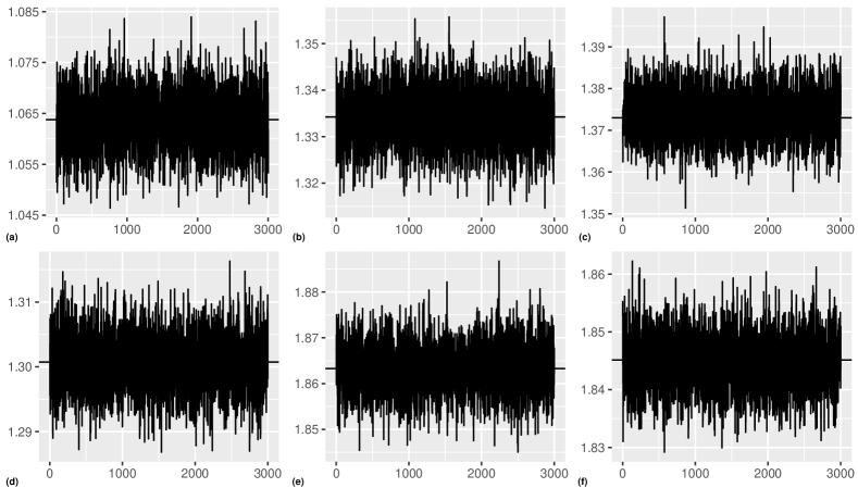
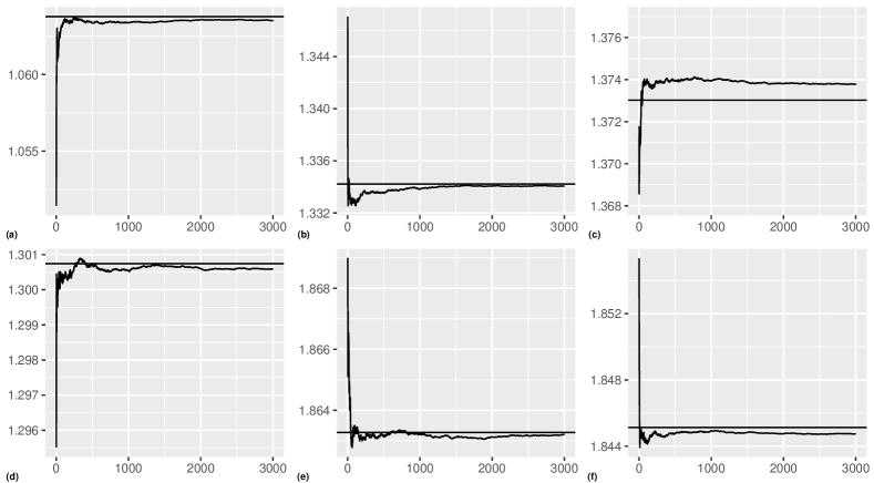
The joint and step-wise methods were both run for 1000 burn-in iterations and then 2000 more follow-up iterations. The hyperparameters were chosen as described towards the end of Section 2.1 (theoretically motivated choices for and and objective inverse-gamma priors for and ). We also consider learning and adaptively by using Beta hyperpriors on and and the results are presented in Tables 8 and 9 of Supplementary Section 10.2. We use traceplots and cumulative average plots to monitor and ensure the convergence of the MCMC. Some of these plots are provided in Figures 1 and 2. The BANS algorithm was run using the default hyperparameter settings in Ha et al. (2020b) again with 1000 burn-in and 2000 more follow-up iterations. DPE and DCPE are optimization algorithms for identifying the relevant posterior mode, and they were run with default settings provided in Deshpande et al. (2019).
Computational performance: We start by evaluating the computational performance of each of the methods. For each of the six combinations from Table 1, we run each of these methods for the 200 replicated data sets and report the average wall clock time. All methods were run on HiPerGator, a high-performance computing cluster at the University of Florida with each node running an Intel Haswell E5-2698 processor. The average wall clock-times are reported in Table 2. The results demonstrate the challenges with scalability for BANS due to the matrix inversion issues discussed in Section 2.2. For the four combinations of with at least predictors and responses, the required 3000 iterations of the MCMC algorithm for a single replication could not be completed in 4 days (mostly, less than 100 iterations were completed). The HS-GHS method also encountered similar issues. For Settings 3, 4, 5 and 6 (where and are both at least 200), the HS-GHS could not complete the required number of iterations in 4 days. In fact, for all these settings less than 150 iterations were completed in 4 days. For all 200 replications in Setting 1 we get an error involving positive definiteness of an intermediate matrix calculation. Hence, results are only provided for Setting 2. On the other hand, we see that both JRNS and Stepwise approaches scale well and can easily handle settings with large and values. As expected, the stepwise approach takes less computing time than the joint approach. While the DPE algorithm also has scalability issues with increasing and , the DCPE algorithm scales very well and is the fastest among all the five algorithms in most settings. In the setting, the stepwise algorithm is faster, and the Joint (JRNS) algorithm also roughly takes the same time as DCPE. However, as noted in Deshpande et al. (2019), the faster speed of DCPE can come at the cost of sub-optimal performance (see also Table 3 below). More importantly, the DCPE algorithm focuses on optimization of the posterior mode, and does not provide samples from the posterior distribution for uncertainty quantification. On the other hand, output from the Joint (JRNS) and Stepwise methods can be used to construct posterior marginal inclusion probabilities and credible intervals. This is demonstrated below in Tables 7, 8 and 9 for the JRNS method.
| Density | Cases | Joint | Stepwise | DPE | DCPE | BANS | HS-GHS | |
| 100 | 6.86 | 6.72 | 1.46 | 0.13 | 3890.11 | PDE | ||
| 100 | 3.79 | 4.48 | 0.67 | 0.05 | 5922.96 | 5811.68 | ||
| 150 | 241.25 | 159.19 | 67295.27 | 62.41 | TO | TO | ||
| 150 | 833.80 | 280.29 | TO | 785.83 | TO | TO | ||
| 100 | 233.93 | 97.57 | 126175.95 | 29.40 | TO | TO | ||
| 200 | 294.20 | 138.50 | 4956.46 | 78.47 | TO | TO | ||
Sparsity selection performance: To assess the sparsity selection performance of the methods developed, the following measures were evaluated after running each method on each of the 200 replicates, and comparing the estimated sparsity patterns with the true sparsity pattern:
| Matthews Correlation Coefficient (MCC) | ||
where TP, TN, FP, FN are the total number of true positive, true negative, false positive and false negative identifications made. The average MCC values for sparsity estimation in and for all methods across all combinations are provided in Tables 3 and 4, respectively.
It can be seen that for sparsity selection in , the JRNS and Stepwise approaches significantly outperfrom DPE and DCPE in most settings. On closer examination of the outputs, one of the reasons appears to be that in some cases the DPE and DCPE estimate by a diagonal matrix, thus failing to identify all non-zero off-diagonal elements. The performance of BANS in the settings where results are available is quite sub-optimal compared to other approaches. For sparsity selection in , the JRNS method gives the best performance. Here the performance of BANS improves compared to sparsity selection, but remains sub-optimal compared to competing approaches. The computationally faster approximations DCPE and Stepwise are in general less accurate than DPE and JRNS, respectively. We have results for HS-GHS only in Setting 2 (due to timeout issues discussed before) and its performance with respect to sparsity selection in that setting is comparable to other methods.
Estimation performance: To assess the estimation performance of the proposed methods, we compute the relative estimation error of the final estimates of and which have been constructed using the majority voting approach described in Section 2.1. The relative estimation errors for are presented in Table 5 and those for are presented in Table 6. As is seen from Table 5 the JRNS method performs very well in all the simulation settings, in fact it is the best performing method in terms of relative estimation error of in most of the settings. The performance of the Stepwise method is also quite competitive here. For estimation of , the transformation described at the end of Section 2.1 was used to ensure positive definiteness of the iterates and the resulting estimate. We have included an additional column in Table 6 for the refitted estimates of as described in Section 2.1. It is evident from Table 6 that the performance of the JRNS method (without refitting) is competitive with the other methods. In Setting 2 where we were able to get HS-GHS output in a reasonable time, its performance is slightly better than JRNS, Stepwise, DPE and DCPE. The refitting based estimates for JRNS exhibit better performance than any other method in most of the settings including Setting 2. Note that for refitting based estimates, the connection to the magnitudes of the entries in the iterates of the JRNS MCMC output, and hence the corresponding credible intervals, is lost (for uncertainty quantification).
| Sparsity | Cases | Joint | Stepwise | DPE | DCPE | BANS | HS-GHS | |
| 100 | 0.783 | 0.778 | 0.593 | 0.576 | 0.374 | PDE | ||
| 100 | 0.821 | 0.820 | 0.708 | 0.623 | 0.305 | 0.831 | ||
| 150 | 0.918 | 0.899 | 0.888 | 0.881 | TO | TO | ||
| 150 | 0.912 | 0.831 | TO | 0.752 | TO | TO | ||
| 100 | 0.867 | 0.846 | 0.533 | 0.571 | TO | TO | ||
| 200 | 0.969 | 0.968 | 0.959 | 0.964 | TO | TO | ||
| Sparsity | Cases | Joint | Stepwise | DPE | DCPE | BANS | HS-GHS | |
| 100 | 1.000 | 1.000 | 1.000 | 1.000 | 0.613 | PDE | ||
| 100 | 1.000 | 1.000 | 1.000 | 1.000 | 0.913 | 0.985 | ||
| 150 | 1.000 | 0.997 | 1.000 | 1.000 | TO | TO | ||
| 150 | 0.998 | 0.770 | TO | 0.938 | TO | TO | ||
| 100 | 0.991 | 0.961 | 0.950 | 0.943 | TO | TO | ||
| 200 | 1.000 | 0.956 | 0.997 | 0.924 | TO | TO | ||
| Sparsity | Cases | Joint | Stepwise | DPE | DCPE | BANS | HS-GHS | |
| 100 | 0.0167 | 0.0169 | 0.0169 | 0.0169 | 0.9323 | PDE | ||
| 100 | 0.0269 | 0.0276 | 0.0275 | 0.0277 | 0.9317 | 0.0308 | ||
| 150 | 0.0154 | 0.0172 | 0.0152 | 0.0153 | TO | TO | ||
| 150 | 0.0038 | 0.0434 | TO | 0.0140 | TO | TO | ||
| 100 | 0.0043 | 0.0141 | 0.0063 | 0.0089 | TO | TO | ||
| 200 | 0.00350 | 0.0116 | 0.0033 | 0.0109 | TO | TO | ||
| Sparsity | Cases | Joint | Joint-Refitted | Stepwise | DPE | DCPE | BANS | HS-GHS | |
| 100 | 0.2444 | 0.1794 | 0.2361 | 0.2300 | 0.2271 | 1.0247 | PDE | ||
| 100 | 0.2475 | 0.1874 | 0.2389 | 0.2424 | 0.2538 | 1.0125 | 0.2180 | ||
| 150 | 0.2197 | 0.1442 | 0.2092 | 0.1429 | 0.1444 | TO | TO | ||
| 150 | 0.2181 | 0.1424 | 0.2306 | TO | 0.1679 | TO | TO | ||
| 100 | 0.2352 | 0.1854 | 0.2262 | 0.2423 | 0.2320 | TO | TO | ||
| 200 | 0.2209 | 0.1159 | 0.2029 | 0.1129 | 0.1100 | TO | TO | ||
Uncertainty quantification based on the generalized posterior distribution: Next, we illustrate uncertainty quantification for JRNS using inclusion probabilities (see Section 2.1) and credible intervals obtained from the generalized posterior distribution. Note that the DPE and DCPE algorithms do not provide posterior samples for this purpose. We first consider the simulation setting where , and randomly choose one out of the replicated data sets. Table 7 shows the estimated marginal inclusion probabilities for selected entries in and using the JRNS algorithm. For the matrix, , entries , , are true positives: they are estimated as non-zero, since all have estimated inclusion probability (the corresponding values were chosen as non-zero for all post burn-in iterations), and their true values in are non-zero. Entry is a false positive: it is estimated as non-zero since the estimated inclusion probability is (the corresponding values were chosen as non-zero for out of post burn-in iterations), but its true value in is zero. Hence, the inclusion probabilities indicate that the decision to classify as non-zero is not supported with the same certainty by the posterior distribution as the decision to classify , , . Finally, entries , are true negatives: they are estimated as zero since the inclusion probabilities and are less than , and their true values in are zero. For the matrix, entries are true positives with estimated marginal inclusion probabilities , entry is false positive with estimated marginal inclusion probability , and entries are true negatives both with estimated marginal inclusion probabilities . The network plots indicating the associations between the predictors and the response variables and also among the response variables for this replication are presented in Figure 3. Note that the BANS algorithm can not provide a full set of iterations for the setting due to computational scalability issues. Hence, inclusion probabilities for the BANS algorithm are not included in Table 7.

| Matrix | Entry | JRNS classification | Inclusion probability | True classification |
|---|---|---|---|---|
| Non-zero | Non-zero | |||
| Non-zero | Non-zero | |||
| Non-zero | Non-zero | |||
| Non-zero | Zero | |||
| Zero | Zero | |||
| Zero | Zero | |||
| Non-zero | Non-zero | |||
| Non-zero | Non-zero | |||
| Non-zero | Non-zero | |||
| Non-zero | Zero | |||
| Zero | Zero | |||
| Zero | Zero |
For a comparative illustration with both JRNS and BANS, we consider the setting. Marginal inclusion probability estimates for selected entries of and for both the joint (JRNS) method and the BANS approach (based on post burn-in iterations) are provided in Table 8. Entries in , and in are true positives for both methods (correctly identified as non-zero), but the inclusion probabilities for BANS are smaller than those of JRNS for all three entries. Entries in and in are falsely identified as non-zero by BANS based on inclusion probabilities greater than , but correctly identified as zero by JRNS. Entry in is correctly identified as non-zero by JRNS with an inclusion probability of while BANS incorrectly identifies it as zero with a low inclusion probability. Other entries in the table are true negatives for both methods (correctly identified as zero), but JRNS has a lower inclusion probability for all as compared to BANS. While the entries reported in Table 8 are just a small subset, we found that the pattern of JRNS having a higher/lower inclusion probability than BANS when the true value is non-zero/zero is repeated for most entries of and . This is not surprising given the significantly better selection performance of JRNS in this setting (see Tables 3 and 4).
| Matrix | Entry | Classification | Inclusion probability | True classification | ||
|---|---|---|---|---|---|---|
| JRNS | BANS | JRNS | BANS | |||
| Non-zero | Non-zero | 0.972 | Non-zero | |||
| Non-zero | Non-zero | 0.765 | Non-zero | |||
| zero | Non-zero | 0.772 | zero | |||
| zero | zero | 0.253 | zero | |||
| zero | zero | 0.2505 | zero | |||
| zero | zero | 0.0495 | zero | |||
| zero | zero | 0.293 | zero | |||
| Non-zero | zero | 0.112 | Non-zero | |||
| Non-zero | Non-zero | 1 | 0.952 | Non-zero | ||
| zero | Non-zero | 0 | 0.5605 | zero | ||
| zero | zero | 0.492 | zero | |||
| zero | zero | 0.4075 | zero | |||
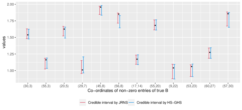
Next, we consider the second simulation setting, where , for a comparison of the empirical coverage probabilities of the posterior credible intervals by JRNS and HS-GHS. For each of 12 true non-zero entries of , and each of the replications, we compute the posterior credible interval obtained by using the relevant sample quantiles of the non-zero values in the post burn-in iterations (for both the methods). The proportion of credible intervals (out of ) which contain the true value gives us an estimate of the coverage probability for each method. Table 9 presents the average coverage over the 200 replicated datasets of true value in the 95 credible intervals for these 12 entries of . For entries, both methods perform very well with respect to including the true value in their corresponding credible intervals. The average coverage probability for JRNS is 0.948, while that for HS-GHS is 0.945. We also provide Figure 4 for a visual comparison of the posterior credible intervals for the non-zero entries of the true in one of the replicates. The plot shows the credible intervals by both methods for all 12 non-zero values in the true for a single data set. In this particular data set, most of the credible intervals by JRNS are in general narrower than the corresponding credible intervals by HS-GHS, though the difference is relatively small. However, for co-ordinate (56,8) the HS-GHS credible interval fails to capture the true value, while the JRNS credible interval contains the true one. Similar patterns were observed in the credible intervals for other replicates.
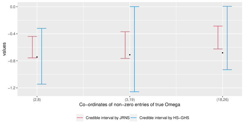
We also obtain credible intervals for the three true non-zero entries of in this setting and computed the coverage probability in a similar process as mentioned above for . For a randomly selected replicate, we plot the credible intervals of the true non-zero entries of by JRNS and HS-GHS in Figure 5 and the average coverage probabilities are listed in Table 9. The credible intervals by JRNS are narrower, however, the comparison of coverage performance is mixed. Due to the narrower credible intervals of JRNS, the true value can sometimes lie just outside the credible interval and hence the coverage probability gets negatively impacted by this. We also obtain credible intervals for the three true non-zero entries of in this setting and computed the coverage probability in a similar process as mentioned above for . For a randomly selected replicate we plot the credible intervals of true non-zero entries of by JRNS and HS-GHS in Figure 5 and the average coverage probabilities are listed in Table 9. The credible intervals by JRNS are narrower, however, the comparison of coverage performance is mixed. Due to the narrower credible intervals of JRNS the true value can sometimes lie just outside the credible interval and hence the coverage probability gets negatively impacted by this.
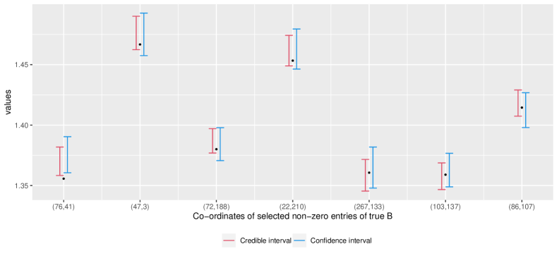
We also consider a simulation setting with , and select a group of entries in which are non-zero. The coverage probabilities for the credible intervals, as described before, are estimated by the proportion of credible intervals (out of 200) containing the true value. The average coverage probability over all true non-zero entries in and over all replications is 0.9422. Recall that the values for BANS and HS-GHS in this setting are not available due to computational scalability issues. Next, we present a comparison between the credible intervals obtained from JRNS and the frequentist confidence intervals obtained from the debiased lasso approach Van de Geer et al. (2014) in Figure 6 for 7 randomly selected coordinates of . The plot indicates that for all of these coordinates the JRNS approach provides narrower and more precise intervals while containing the corresponding true values for most of these coordinates. The codes implementing the two proposed methods, namely the JRNS and the Stepwise methods are available at https://github.com/srijata06/JRNS_Stepwise.
| coordinates | JRNS | HS-GHS | |
| (30,3) | 0.940 | 0.945 | |
| (55,3) | 0.945 | 0.930 | |
| (20,5) | 0.955 | 0.925 | |
| (29,7) | 0.970 | 0.970 | |
| (45,8) | 0.930 | 0.950 | |
| (56,8) | 0.940 | 0.950 | |
| (17,14) | 0.945 | 0.935 | |
| (55,20) | 0.940 | 0.945 | |
| (9,22) | 0.945 | 0.925 | |
| (53,23) | 0.970 | 0.980 | |
| (60,27) | 0.955 | 0.945 | |
| (57,30) | 0.940 | 0.935 | |
| (2,8) | 0.607 | 0.865 | |
| (3,19) | 0.938 | 0.800 | |
| (18,26) | 0.778 | 0.810 |
5 Analysis of TCGA cancer data
| Cancer type | ||||
|---|---|---|---|---|
| 1 | READ | 121 | 73 | 76 |
| 2 | LUAD | 356 | 73 | 76 |
| 3 | COAD | 338 | 73 | 76 |
| 4 | LUSC | 309 | 73 | 86 |
| 5 | OV | 227 | 73 | 77 |
| 6 | SKCM | 333 | 73 | 76 |
| 7 | UCEC | 393 | 73 | 77 |
To further illustrate the performance of the proposed methods, we present results from the analysis of cancer data from TCGA (The Cancer Genome Atlas). We consider data for 7 different TCGA tumor types: colon adenocarcinoma (COAD), lung adenocarcinoma (LUAD), lung squamous cell carcinoma (LUSC), ovarian serous cystadenocarcinoma (OV), rectum adenocarcinoma (READ) skin cutaneous melanoma (SKCM) and uterine corpus endometrial carcinoma (UCEC). For each of these cancer types we have mRNA expression data and RPPA-based proteomic data. As mentioned in the introduction, since mRNA is translated to protein, it is natural to consider protein expression data to be the response variable and the mRNA expression data to be the predictors. The sample size , number of predictors and the number of response variables for the 7 data sets corresponding to each cancer type are given in Table 10.
| Gene | Protein | Inclusion Probability | |
|---|---|---|---|
| 1 | X1 | 1 | 0.98 |
| 2 | X2 | 2 | 1.00 |
| 3 | X64 | 2 | 0.88 |
| 4 | X60 | 3 | 0.78 |
| 5 | X4 | 4 | 1.00 |
| 6 | X32 | 4 | 0.53 |
| 7 | X5 | 5 | 1.00 |
| 8 | X16 | 5 | 0.56 |
| 9 | X6 | 6 | 1.00 |
| 10 | X7 | 7 | 1.00 |
| 11 | X20 | 7 | 0.98 |
| 12 | X8 | 8 | 1.00 |
| 13 | X56 | 9 | 0.96 |
| 14 | X60 | 9 | 1.00 |
| 15 | X11 | 10 | 1.00 |
| 16 | X11 | 11 | 1.00 |
| 17 | X20 | 11 | 0.76 |
| 18 | X12 | 12 | 1.00 |
| 19 | X13 | 13 | 1.00 |
| 20 | X14 | 13 | 0.91 |
| 21 | X16 | 13 | 0.63 |
| 22 | X70 | 14 | 0.79 |
| 23 | X15 | 16 | 1.00 |
| 24 | X40 | 16 | 0.72 |
| 25 | X10 | 17 | 0.94 |
| 26 | X16 | 17 | 1.00 |
| 27 | X17 | 18 | 1.00 |
| Gene | Protein | Inclusion Probability | |
|---|---|---|---|
| 28 | X68 | 18 | 0.52 |
| 29 | X18 | 19 | 1.00 |
| 30 | X11 | 20 | 0.69 |
| 31 | X17 | 21 | 0.72 |
| 32 | X21 | 21 | 1.00 |
| 33 | X6 | 22 | 0.86 |
| 34 | X21 | 24 | 0.75 |
| 35 | X24 | 24 | 1.00 |
| 36 | X23 | 25 | 1.00 |
| 37 | X28 | 25 | 0.81 |
| 38 | X63 | 25 | 0.66 |
| 39 | X70 | 25 | 0.97 |
| 40 | X10 | 26 | 0.54 |
| 41 | X8 | 27 | 0.60 |
| 42 | X11 | 27 | 0.89 |
| 43 | X27 | 27 | 1.00 |
| 44 | X28 | 28 | 1.00 |
| 45 | X58 | 28 | 0.98 |
| 46 | X29 | 29 | 1.00 |
| 47 | X64 | 30 | 0.89 |
| 48 | X17 | 31 | 1.00 |
| 49 | X31 | 31 | 1.00 |
| 50 | X32 | 31 | 0.81 |
| 51 | X42 | 32 | 0.99 |
| 52 | X34 | 34 | 1.00 |
| 53 | X70 | 34 | 0.83 |
| 54 | X33 | 35 | 0.99 |
| Gene | Protein | Inclusion Probability | |
|---|---|---|---|
| 55 | X35 | 35 | 1.00 |
| 56 | X36 | 37 | 0.51 |
| 57 | X31 | 38 | 0.58 |
| 58 | X37 | 38 | 1.00 |
| 59 | X38 | 39 | 1.00 |
| 60 | X25 | 40 | 0.65 |
| 61 | X39 | 40 | 1.00 |
| 62 | X8 | 41 | 0.53 |
| 63 | X47 | 41 | 1.00 |
| 64 | X24 | 43 | 0.53 |
| 65 | X43 | 43 | 1.00 |
| 66 | X44 | 44 | 0.92 |
| 67 | X46 | 44 | 0.94 |
| 68 | X11 | 47 | 0.96 |
| 69 | X47 | 47 | 1.00 |
| 70 | X36 | 49 | 0.91 |
| 71 | X50 | 50 | 0.71 |
| 72 | X6 | 52 | 0.81 |
| 73 | X61 | 53 | 1.00 |
| 74 | X68 | 53 | 0.88 |
| 75 | X72 | 56 | 0.96 |
| 76 | X58 | 57 | 1.00 |
| 77 | X60 | 57 | 1.00 |
| 78 | X15 | 58 | 0.81 |
| 79 | X58 | 58 | 1.00 |
| 80 | X28 | 59 | 0.78 |
| 81 | X58 | 59 | 1.00 |
| Gene | Protein | Inclusion Probability | |
|---|---|---|---|
| 82 | X59 | 59 | 0.92 |
| 83 | X61 | 61 | 0.51 |
| 84 | X6 | 62 | 0.64 |
| 85 | X29 | 63 | 0.98 |
| 86 | X62 | 63 | 1.00 |
| 87 | X70 | 63 | 1.00 |
| 88 | X63 | 64 | 1.00 |
| 89 | X33 | 65 | 0.90 |
| 90 | X63 | 65 | 1.00 |
| 91 | X63 | 66 | 1.00 |
| 92 | X17 | 68 | 0.83 |
| 93 | X46 | 68 | 0.86 |
| 94 | X24 | 69 | 0.78 |
| 95 | X11 | 71 | 0.52 |
| 96 | X57 | 71 | 0.64 |
| 97 | X67 | 71 | 0.94 |
| 98 | X59 | 72 | 0.51 |
| 99 | X69 | 73 | 1.00 |
| 100 | X3 | 74 | 0.53 |
| 101 | X70 | 74 | 1.00 |
| 102 | X71 | 74 | 0.99 |
| 103 | X14 | 75 | 0.85 |
| 104 | X72 | 75 | 1.00 |
| 105 | X73 | 76 | 1.00 |
We carry out a separate data analysis for each of the seven cancer types. For JRNS and the Stepwise estimation methods the Gibbs samplers were run for 1000 iterations for burn-in followed by additional 2000 iterations for calculating the regression coefficients and the precision matrices. As noted earlier, DPE and DCPE do not provide uncertainty quantification. While BANS does provide uncertainty quantification, computationally it takes a prohibitively long time with the above values. In Ha et al. (2020b), this dataset was analyzed but the dataset for each cancer type was further broken based on pathway information, which significantly reduces the dimensionality of the problem.
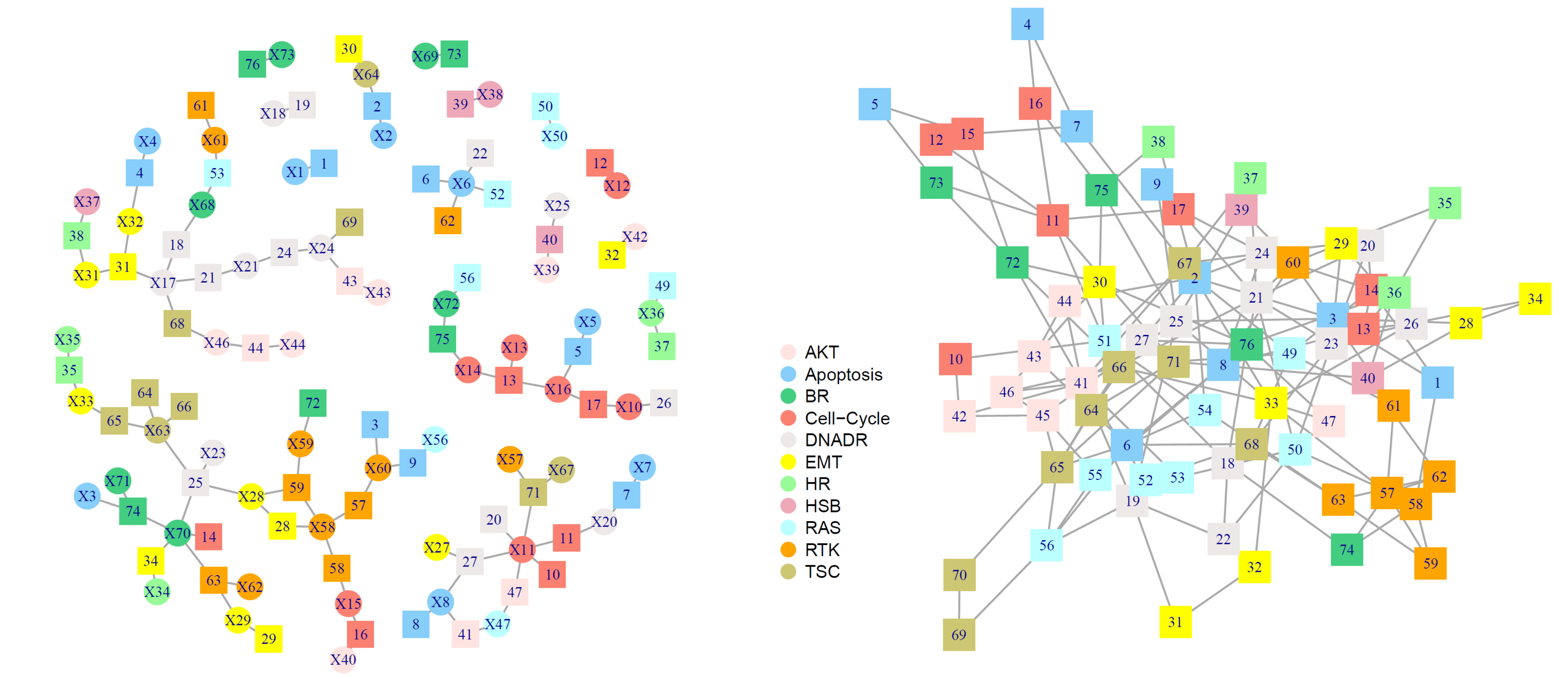
We present the estimated network plots obtained using JRNS depicting (1) the associations between mRNA and proteins and (2) that among the proteins for the LUAD cancer type in Figure 7. The indices/serial numbers for genes and proteins for the LUAD dataset are given in Table 13 in the Appendix. Figure 7 depicts the sparsity estimates of and for the LUAD type cancer based on a 0.5 cutoff for the inclusion probabilities. The genes and proteins are mapped to their respective functional pathways to aid interpretation. The list of pathways and the corresponding genes for each of the pathways is listed in Table 14 in the Appendix. For the associations encoded in matrix (see left panel of Figure 7), we see genes and proteins from the following pathways to be involved : RTK, EMT, Cell Cycle and Apoptosis. The results are broadly consistent with known functional mechanisms for the disease including stimulation of RTK to activate downstream signaling that encodes EMT’s inducing transcription factors Gonzalez and Medici (2014). The epithelial mesenchymal transition (EMT) is an essential mechanism that contributes to the progression in cancer and involves apoptotic responses and the cell cycle, all elements captured in some of the connections depicted in the Figure. Further, we see similar connections at the protein expression network in the right panel of Figure 7. One can also see that there are strong connections within members of the same pathway, as well as cross-talk with members of other pathways. We particularly focus on the LUAD network plots here as it shows some very interesting biological connections. The network plots for the other cancer types are included in the Supplementary file.
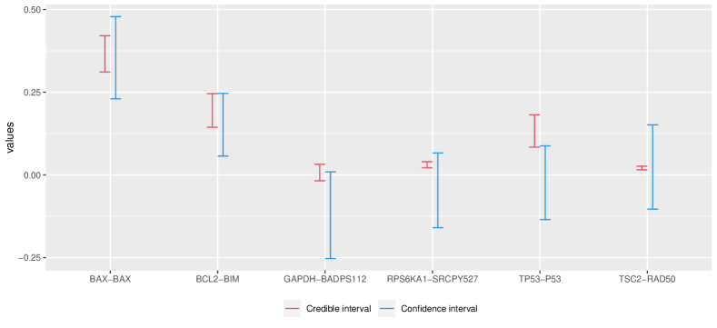
Next, we present Figure 8 which depicts the coverage of the credible intervals by JRNS and the confidence intervals by Debiased Lasso for six randomly selected entries of for the lung adenocarcinoma (LUAD) cancer data. We randomly selected 6 gene-protein coordinates in . Here the credible intervals are not only much shorter than the corresponding confidence intervals, but in most cases are subsets of their corresponding confidence intervals.
| JRNS | Stepwise | DPE | DCPE | |
|---|---|---|---|---|
| READ | 0.509 | 0.513 | 0.516 | 0.513 |
| LUAD | 0.878 | 0.869 | 0.874 | 0.876 |
| LUSC | 0.838 | 0.839 | 0.834 | 0.836 |
| COAD | 0.887 | 0.881 | 0.886 | 0.884 |
| OV | 0.778 | 0.779 | 0.774 | 0.779 |
| SKCM | 0.859 | 0.860 | 0.859 | 0.860 |
| UCEC | 0.919 | 0.912 | 0.917 | 0.919 |
We also compare the prediction accuracy of the proposed methods with DPE and DCPE. Default settings were chosen for these methods as mentioned in Section 4. Results for HSGHS could not be obtained since we get the same error involving positive definiteness of an intermediate matrix calculation here as well. For prediction evaluation purposes, we perform a 5-fold cross validation in which we randomly divide the data set for each cancer type into 5 parts. The model for each of the listed approaches in Table 12 is built 5 times, each time using one of the parts as the test set and the rest as the training set. The average prediction error is then normalized with respect to that corresponding to the vanilla regression method ( separate response-specific linear models). A relative prediction error less than implies that the corresponding method has better prediction performance than the vanilla regression approach. All the relative prediction errors are listed in Table 12. The results show that the proposed methods have a very similar and competitive predictive performance compared to DPE and DCPE, while additionally providing uncertainty quantification by sampling from the posterior distribution.
6 Discussion
In this paper, we use a biconvex generalized likelihood function along with sparsity inducing spike-and-slab prior distributions for joint sparsity selection and estimation of the regression coefficient and error covariance matrices in multivariate linear regression models. The proposed JRNS and Stepwise algorithms are significantly faster than related (generalized) Bayesian methods both due to the simpler algebraic structure of the generalized likelihood used and also due to more efficient MCMC implementation (as discussed in Section 2.2), provide samples from the generalized posterior distribution for uncertainty quantification, and perform competitively in terms of selection/estimation performance in simulated data settings and in the TCGA cancer data application.
Intuitively, the joint JRNS approach should provide better accuracy than the Stepwise approach as it utilizes the cross-correlations among the errors in estimation of (while the Stepwise approach ignores them). This is borne out in the simulations, especially for Setting 4 with . However, theoretical analysis of the joint generalized posterior of for the JRNS approach is much more complicated than the corresponding analysis for the Stepwise approach. One possible direction of future enquiry is to establish high-dimensional posterior consistency results for the joint JRNS approach (analogous to those in Theorem 1 for the Stepwise approach). Another possible future direction would be to explore the use of the biconvex generalized likelihood functions along with continuous shrinkage prior distributions, such as the Horseshoe one and study the computational and theoretical properties of such an approach.
Appendix: Pathways for TCGA cancer data
Table 13 listes the indices of all the genes and proteins in the LUAD cancer data and Table 14 lists all the pathways that have been considered in the analysis of the TCGA cancer data in Section 5 and their gene members.
| Gene | Protein | |
|---|---|---|
| 1 | BAK1 | BAK |
| 2 | BAX | BAX |
| 3 | BID | BID |
| 4 | BCL2L11 | BIM |
| 5 | CASP7 | CASPASE7CLEAVEDD198 |
| 6 | BAD | BADPS112 |
| 7 | BCL2 | BCL2 |
| 8 | BCL2L1 | BCLXL |
| 9 | BIRC2 | CIAP |
| 10 | CDK1 | CDK1 |
| 11 | CCNB1 | CYCLINB1 |
| 12 | CCNE1 | CYCLINE1 |
| 13 | CCNE2 | CYCLINE2 |
| 14 | CDKN1B | P27PT157 |
| 15 | PCNA | P27PT198 |
| 16 | FOXM1 | PCNA |
| 17 | TP53BP1 | FOXM1 |
| 18 | ATM | 53BP1 |
| 19 | BRCA2 | ATM |
| 20 | CHEK1 | CHK1PS345 |
| 21 | CHEK2 | CHK2PT68 |
| 22 | XRCC5 | KU80 |
| 23 | MRE11A | MRE11 |
| 24 | TP53 | P53 |
| 25 | RAD50 | RAD50 |
| 26 | RAD51 | RAD51 |
| 27 | XRCC1 | XRCC1 |
| 28 | FN1 | FIBRONECTIN |
| 29 | CDH2 | NCADHERIN |
| 30 | COL6A1 | COLLAGENVI |
| 31 | CLDN7 | CLAUDIN7 |
| 32 | CDH1 | ECADHERIN |
| 33 | CTNNB1 | BETACATENIN |
| 34 | SERPINE1 | PAI1 |
| 35 | ESR1 | ERALPHA |
| 36 | PGR | ERALPHAPS118 |
| 37 | AR | PR |
| 38 | INPP4B | AR |
| Gene | Protein | |
|---|---|---|
| 39 | GATA3 | INPP4B |
| 40 | AKT1 | GATA3 |
| 41 | AKT2 | AKTPS473 |
| 42 | AKT3 | AKTPT308 |
| 43 | GSK3A | GSK3ALPHABETAPS21S9 |
| 44 | GSK3B | GSK3PS9 |
| 45 | AKT1S1 | PRAS40PT246 |
| 46 | TSC2 | TUBERINPT1462 |
| 47 | PTEN | PTEN |
| 48 | ARAF | ARAFPS299 |
| 49 | JUN | CJUNPS73 |
| 50 | RAF1 | CRAFPS338 |
| 51 | MAPK8 | JNKPT183Y185 |
| 52 | MAPK1 | MAPKPT202Y204 |
| 53 | MAPK3 | MEK1PS217S221 |
| 54 | MAP2K1 | P38PT180Y182 |
| 55 | MAPK14 | P90RSKPT359S363 |
| 56 | RPS6KA1 | YB1PS102 |
| 57 | YBX1 | EGFRPY1068 |
| 58 | EGFR | EGFRPY1173 |
| 59 | ERBB2 | HER2PY1248 |
| 60 | ERBB3 | HER3PY1298 |
| 61 | SHC1 | SHCPY317 |
| 62 | SRC | SRCPY416 |
| 63 | EIF4EBP1 | SRCPY527 |
| 64 | RPS6KB1 | 4EBP1PS65 |
| 65 | MTOR | 4EBP1PT37T46 |
| 66 | RPS6 | 4EBP1PT70 |
| 67 | RB1 | P70S6KPT389 |
| 68 | CAV1 | MTORPS2448 |
| 69 | MYH11 | S6PS235S236 |
| 70 | RAB11A | S6PS240S244 |
| 71 | RAB11B | RBPS807S811 |
| 72 | GAPDH | CAVEOLIN1 |
| 73 | RBM15 | MYH11 |
| 74 | RAB11 | |
| 75 | GAPDH | |
| 76 | RBM15 |
| Pathway | Genes | |
|---|---|---|
| 1 | AKT/PI3K | AKT1, AKT2, AKT3, GSK3A, GSK3B, CDKN1B, AKT1S1, TSC2, INPP4B, PTEN |
| 2 | Apoptosis | BAK1, BAX, BID, BCL2L11, CASP7, BAD, BCL2, BCL2L1, BIRC2 |
| 3 | Breast Reactive | CAV1, MYH11, RAB11A, RAB11B, CTNNB1, GAPDH, RBM15 |
| 4 | Cell Cycle | CDK1, CCNB1, CCNE1, CCNE2, CDKN1B, PCNA, FOXM1 |
| 5 | DNA damage response | TP53BP1, ATM, BRCA2, CHEK1, CHEK2, XRCC5, MRE11A, TP53,RAD50, RAD51, XRCC1 |
| 6 | EMT | FN1, CDH2, COL6A1, CLDN7, CDH1, CTNNB1, SERPINE1 |
| 7 | Hormone Receptor | ES1, EGR, PR |
| 8 | Hormone Signaling (Breast) | INPP4B, GATA3, BCL2 |
| 9 | RAS | ARAF, JUN, RAF1, MAPK8, MAPK1, MAPK3, MAP2K1, MAPK14, RPS6KA1, YBX1 |
| 10 | RTK | EGFR, ERBB2, ERBB3, SHC1, SRC |
| 11 | TSC | EIF4EBP1, RPS6KB1, MTOR, RPS6, RB1 |
7 Details of the proof of Theorem 1(a), 1(b)
7.1 Assumptions required for Theorem 1(a), 1(b)
We recall that and represents the sparsity indicator of . Also, denotes the sparsity indicator of the true parameter . Let denote the -th column of and be the number of non-zero entries in . We will consider only the models with sparsity indicator for which for all where is a realistic model cut-off size (See Assumption A2). Below, for a matrix we will use the operator norm , the Frobenius norm and the norms and . Let be an arbitrarily fixed constant. Also, we define
where is the -th element of .
Assumption A1.
There exists and not depending on such that the eigenvalues of all submatrices of are bounded below and above by and respectively, and
where is the -th diagonal element of .
Assumption A2.
for some and and where for some
Assumption A3.
The slab variance satisfies where denotes the -th column of .
Assumption A4.
7.2 Proof of Theorem 1(a)
Let denote the posterior probability of . Given the true model with sparsity indicator and another arbitrary model with sparsity indicator , the ratio of posterior probabilities can be shown to satisfy
| (15) | ||||
| (16) |
Here represents the submatrix of consisting of columns corresponding to the active indices in , represents the identity matrix of order and
The derivation of (7.2) follows from computations similar to those given in Ghosh et al. (2021). Let denote the projection matrix into the column space of and
We define four events below and show that they occur with probability tending to 1.
where represents the sub-matrix of R consisting of rows and columns corresponding to the active indices in
We also define
Using Theorem 6.2.1 from Vershynin (2018) and Lemma F.2 from Basu and Michailidis (2015) we get
Hence
| (17) |
Here we use an upper bound for as obtained in the proof of Lemma 4.1 of Cao et al. (2020). Using arguments similar to those in the proof for it can be shown that and that
It then follows that
| (20) |
We now state and prove two lemmas which will be used to prove Theorem 1(a).
Lemma 2.
If for a particular , then there exists (not depending on or ) such that for all on the set , we have
Proof.
Lemma 3.
If for a particular is such that , then there exists (not depending on or ) such that for all on the set , we have
if , and
if .
Proof.
Let . Then
| (28) |
Using (7.2) and (7.2) it can be shown that
and hence we get
| (29) |
CASE I: For all sufficiently large and Thus, on we have
| (30) |
We have already shown in the proof of Lemma 1 that
As for all large , using arguments similar to the proof of Lemma 1 it can be shown that on we have
| (31) |
On ,
and
for Then on ,
| (32) |
for some appropriate constant . Hence from (7.2) we have
| (33) |
by Assumption A2.
CASE II: Let Also, let and denote the vectors consisting of the elements of ( the -th column of ) which correspond to the active indices of , and respectively. We first find a lower bound for . Using Woodbury’s identity it can be shown that
| (34) |
We show that the second term is the dominating term and is bounded below by where is as in Assumption A2. Without loss of generality, we assume that is composed as where
| (35) |
Hence,
| (36) |
Now by Lemma S1.4 of Ghosh et al. (2021) there exists a vector such that
where and .
On we have
| (37) |
by Assumption A2. Thus,
By Assumption A4, on the set ,
Now, since , we have
| (39) |
for some appropriate constant . Now
| (40) |
∎
Proof of Theorem 1(a). We first prove that
. Let and be as in Lemmas 1 and 2 and . Then for all and , on the set ,
| (42) | |||||
by Lemmas 1 and 2. In order to find a bound for (42), we use the inequalities , and for . We also note that so that and for , we have and . We then have
and therefore,
Now
As , we get as .
Now we recall that
and is defined as 1 if and if Let .
For .
Thus for .
For .
Thus for . Then
| (43) |
7.3 Proof of Theorem 1(b)
Next we prove the theorem on estimation consistency for where we show that there exists a constant such that
where and denotes the posterior distribution.
For each , let denote the vector of dimension consisting of the non-zero entries of given the true sparsity pattern and or simply denote the vector consisting of the non-zero entries of , the column of . Let be a matrix whose -th column, is given by the posterior mean
Let be the vector of dimension consisting of the non-zero entries of . Then it can be shown that
First we note that for any ,
| (44) |
Thus it is enough to show that
since it is proved earlier that . Also it can be shown that
| (45) |
where and the maximum is over those for which . Further,
| (46) |
The posterior distribution of and are given by
Now
| (47) |
where is a standard normal vector.
| (48) |
We set
Similar to the set defined above, it can be shown that for some suitably chosen constants and . Then for a fixed on the set ,
and hence
To bound the third term in the RHS of (7.3) we recall the distribution of and use a slight modification of Remark S1.1 of Ghosh et al. (2021) with replaced by wherein we show both the shape and scale of the Inverse gamma distribution are of appropriate order.
We set and note that . Now on , by arguments used in proving equation (7.2)
and also . Then by choosing properly we can make for all large .
Using Corollary 5.35 in Vershynin (2018) one can show that
Then setting and choosing such that one can show that
| (49) |
Thus we get
| (50) |
Finally we obtain an upper bound for the second term, in (7.3). To that end we first note for each
| (51) |
Now, on using Assumption A3 we have
| (52) |
and on we have
| (53) |
| (56) |
8 Details of proof of Theorem 1(c)
8.1 Assumptions required for Theorem 1(c)
Assumption B1.
as
where denotes the number of non-zero entries in the upper triangle of .
Assumption B2.
There exists such that
Assumption B3.
, as
where denotes the smallest absolute value among all the off-diagonal entries of .
Assumption B4.
We choose where
where is an appropriately chosen constant.
8.2 Proof of Theorem 1(c)
A Bayesian approach has been developed in Jalali et al. (2020) for sparse estimation of the error precision matrix in a high-dimensional setting using spike and slab priors and the regression based generalized likelihood function of Khare et al. (2015). Their results are applicable in our case if the regression coefficient matrix is assumed to known. The expression for the posterior distribution of the sparsity pattern of , as obtained in Jalali et al. (2020) depends on the estimate of the variance-covariance matrix . However, in our case is unknown and so we estimate it by as obtained in Step 1 of the Stepwise method and replace by . Below we provide a bound for .
Let denote the true value of and , and be as defined above in Section 7. Our final estimate of is obtained from , replacing by its estimate .
Now,
| (57) |
and on we have
Since is obtained from , replacing by its estimate , it follows from Theorem 1(a) and (8.2) that with -probability tending to one,
| (61) |
Next we provide a bound for using the bound provided in (61). We note that can be decomposed as follows:
| (62) |
We have
and for each on ,
Hence,
We also have
and for each ,
For each on ,
So, for each ,
and hence,
Now from equation (62), on ,
| (63) |
for some appropriate constant c.
Using the fact that and are good approximations of and respectively and using straightforward modifications of the arguments of Jalali et al. (2020) and some additional arguments we show that the posterior distribution of is consistent in the sense that
Finally the part (c) of Theorem 1 follows from this result using arguments similar to that leading to (7.2) above in the proof of part (a).
9 Detailed algorithm of JRNS
10 Additional simulation results
10.1 Sparsity selection performance
In the main paper we have presented the average MCC values for sparsity estimation in both and based on 200 replicated datasets for all the methods, namely JRNS(Joint), Stepwise approach, DPE, DCPE and BANS. We considered a variety of combinations of listed in Table 1 of the main paper. Here we present tables with average values of sensitivity and specificity for sparsity estimation in both and . We also present average values of relative norm for sparsity estimation in which is defined as where denotes the Frobenius norm of a matrix.
For sparsity selection in , we see that the JRNS and Stepwise approaches perform much better than DCPE and DPE with respect to average sensitivity values. For specificity all the methods have values very close to 1. Though BANS performs competitively with respect to specificity, in terms of sensitivity, it is clearly outperformed by the JRNS and Stepwise methods. For sparsity selection in , the JRNS algorithm shows the best performance in most of the settings and the values for the different measures for DPE and DCPE are very close to the corresponding values for JRNS and Stepwise algorithms. For BANS the sensitivity values improve here but it still has sub-optimal performance with respect to relative norm of the estimate of .
| Sparsity | Cases | Joint | Stepwise | DPE | DCPE | BANS | HSGHS | |
| 100 | 0.6817 | 0.6967 | 0.2142 | 0.2233 | 0.4817 | PDE | ||
| 100 | 0.7267 | 0.7383 | 0.1550 | 0.0283 | 0.2650 | 0.7150 | ||
| 150 | 0.9290 | 0.9340 | 0.7876 | 0.7780 | TO | TO | ||
| 150 | 0.9450 | 0.8753 | TO | 0.7447 | TO | TO | ||
| 100 | 0.8480 | 0.8620 | 0.2924 | 0.3303 | TO | TO | ||
| 200 | 0.9780 | 0.9805 | 0.9265 | 0.9323 | TO | TO | ||
| Sparsity | Cases | Joint | Stepwise | DPE | DCPE | BANS | HS-GHS | |
| 100 | 0.9997506 | 0.9996344 | 1.0000000 | 1.0000000 | 0.9961338 | PDE | ||
| 100 | 0.9997338 | 0.9995949 | 0.9999884 | 1.0000000 | 0.9963194 | 0.9997569 | ||
| 150 | 0.9999019 | 0.9998506 | 0.9999990 | 0.9999995 | TO | TO | ||
| 150 | 0.9999779 | 0.9999199 | TO | 0.9998398 | TO | TO | ||
| 100 | 0.9998888 | 0.9998159 | 0.9999970 | 0.9999975 | TO | TO | ||
| 200 | 0.9999059 | 0.9998667 | 0.9999972 | 0.9999977 | TO | TO | ||
| Sparsity | Cases | Joint | Stepwise | DPE | DCPE | BANS | HS-GHS | |
| 100 | 1.0000000 | 1.0000000 | 1.0000000 | 1.0000000 | 0.9991667 | PDE | ||
| 100 | 1.0000000 | 1.0000000 | 1.0000000 | 1.0000000 | 0.9975000 | 1.000000 | ||
| 150 | 1.000000 | 1.000000 | 1.0000000 | 0.9999992 | TO | TO | ||
| 150 | 1.0000000 | 1.0000000 | TO | 1.0000000 | TO | TO | ||
| 100 | 1.0000000 | 1.0000000 | 1.0000000 | 1.0000000 | TO | TO | ||
| 200 | 1.0000000 | 1.0000000 | 1.0000000 | 1.0000000 | TO | TO | ||
| Sparsity | Cases | Joint | Stepwise | DPE | DCPE | BANS | HS-GHS | |
| 100 | 0.9999972 | 1.0000000 | 1.0000000 | 1.0000000 | 0.9941304 | PDE | ||
| 100 | 1.0000000 | 1.0000000 | 1.0000000 | 1.0000000 | 0.9987360 | 0.9997791 | ||
| 150 | 0.9999977 | 0.9999932 | 1.0000000 | 0.9999992 | TO | TO | ||
| 150 | 0.9999977 | 0.9996601 | TO | 0.9999030 | TO | TO | ||
| 100 | 0.9999970 | 0.9999735 | 0.9999557 | 0.9999825 | TO | TO | ||
| 200 | 0.9999987 | 0.9999627 | 0.9999990 | 0.9999575 | TO | TO | ||
10.2 Hyperparameter selection
The important issue of selection of hyperparameters was briefly discussed in Section 2 of the main paper. As mentioned there, the theoretical results of our paper and also those of Cao et al. (2019) and Narisetty and He (2014) motivated us to take and . In order to see how sensitive our results are with respect to changes in the values of the hyperparameters around our choices, we performed simulation experiments for different choices of and for the setting where and the number of non-zero entries in and among the off-diagonal entries of are and respectively. The values of MCC for sparsity selection of and and relative estimation error of for different values of and together with our choices of and as well as different values of the sample size are presented in Tables 19 - 21. The results in these tables reaffirm the intuition that especially as the sample size grows, there are no significant changes in the performance of the estimators as we vary the values of the hyperparameters and .
| Sample size | |||||||
|---|---|---|---|---|---|---|---|
| JRNS | Stepwise | JRNS | Stepwise | JRNS | Stepwise | ||
| 50 | 0.456611 | 0.195824 | 0.443757 | 0.191426 | 0.413763 | 0.185339 | |
| 0.522697 | 0.407968 | 0.510742 | 0.396833 | 0.462008 | 0.356453 | ||
| 0.630093 | 0.626606 | 0.626373 | 0.628004 | 0.578496 | 0.605354 | ||
| 100 | 0.824727 | 0.788363 | 0.816666 | 0.801548 | 0.758186 | 0.787223 | |
| 0.861820 | 0.829216 | 0.854171 | 0.847995 | 0.809472 | 0.845547 | ||
| 0.852824 | 0.844891 | 0.864933 | 0.859695 | 0.868123 | 0.871109 | ||
| 150 | 0.944332 | 0.891047 | 0.944369 | 0.913404 | 0.926108 | 0.937398 | |
| 0.936696 | 0.890740 | 0.943541 | 0.912652 | 0.942260 | 0.945645 | ||
| 0.897044 | 0.891543 | 0.922895 | 0.918023 | 0.948174 | 0.948327 | ||
| 200 | 0.958262 | 0.906148 | 0.967857 | 0.929079 | 0.969988 | 0.968598 | |
| 0.944422 | 0.908759 | 0.958733 | 0.932000 | 0.971172 | 0.969177 | ||
| 0.911446 | 0.908679 | 0.937298 | 0.930596 | 0.969767 | 0.969714 | ||
| Sample size | |||||||
|---|---|---|---|---|---|---|---|
| JRNS | Stepwise | JRNS | Stepwise | JRNS | Stepwise | ||
| 50 | 0.549165 | 0.088672 | 0.542708 | 0.088634 | 0.543439 | 0.088686 | |
| 0.592646 | 0.161716 | 0.590881 | 0.161653 | 0.590786 | 0.162460 | ||
| 0.713135 | 0.819988 | 0.714307 | 0.820428 | 0.715335 | 0.818886 | ||
| 100 | 0.488290 | 0.147177 | 0.487633 | 0.147078 | 0.489134 | 0.147308 | |
| 0.635307 | 0.282160 | 0.632513 | 0.281971 | 0.632951 | 0.282221 | ||
| 0.924696 | 0.870234 | 0.924777 | 0.868219 | 0.922867 | 0.868982 | ||
| 150 | 0.412558 | 0.205877 | 0.412212 | 0.205819 | 0.412529 | 0.205947 | |
| 0.565750 | 0.330461 | 0.566835 | 0.330390 | 0.565658 | 0.330595 | ||
| 0.958730 | 0.892018 | 0.957689 | 0.893823 | 0.958287 | 0.894166 | ||
| 200 | 0.383624 | 0.248326 | 0.384346 | 0.248388 | 0.383731 | 0.248295 | |
| 0.520121 | 0.374873 | 0.521217 | 0.374745 | 0.521213 | 0.374880 | ||
| 0.934772 | 0.888740 | 0.934523 | 0.889443 | 0.936059 | 0.888556 | ||
| Sample size | |||||||
|---|---|---|---|---|---|---|---|
| Joint | Stepwise | Joint | Stepwise | Joint | Stepwise | ||
| 50 | 0.079190 | 0.204494 | 0.082342 | 0.204656 | 0.084490 | 0.204276 | |
| 0.041919 | 0.145363 | 0.041923 | 0.146736 | 0.042020 | 0.145176 | ||
| 0.031765 | 0.021795 | 0.031596 | 0.021790 | 0.031658 | 0.021832 | ||
| 100 | 0.029408 | 0.104857 | 0.029514 | 0.105318 | 0.029476 | 0.104686 | |
| 0.021651 | 0.055278 | 0.021727 | 0.055390 | 0.021742 | 0.055232 | ||
| 0.011085 | 0.012678 | 0.011081 | 0.012737 | 0.011161 | 0.012734 | ||
| 150 | 0.028091 | 0.060263 | 0.028124 | 0.060331 | 0.028103 | 0.060318 | |
| 0.019697 | 0.039141 | 0.019654 | 0.039091 | 0.019711 | 0.039098 | ||
| 0.007320 | 0.009555 | 0.007345 | 0.009527 | 0.007328 | 0.009517 | ||
| 200 | 0.026405 | 0.044825 | 0.026352 | 0.044801 | 0.026420 | 0.044862 | |
| 0.018945 | 0.030533 | 0.018890 | 0.030560 | 0.018888 | 0.030558 | ||
| 0.006642 | 0.008472 | 0.006657 | 0.008449 | 0.006610 | 0.008475 | ||
For and we have also suggested taking Beta priors. The Beta prior in particular is attractive due to conditional conjugacy and the resulting computational simplicity of the conditional updates for and . Below in Tables 22 and 23 we present the sparsity selection performance in and based on the MCC metric using Beta(1,1), i.e., uniform hyper-priors on and for all simulation settings for both the JRNS and Stepwise algorithms.
| Sparsity | Cases | Joint | Joint | Stepwise | Stepwise | ||
| fixed , | Beta(1,1) hyperprior | fixed , | Beta(1,1) hyperprior | ||||
| 100 | 1.000 | 1.000 | 1.000 | 1.000 | |||
| 100 | 1.000 | 1.000 | 1.000 | 1.000 | |||
| 150 | 1.000 | 1.000 | 0.997 | 1.000 | |||
| 150 | 0.998 | 1.000 | 0.770 | 0.982 | |||
| 100 | 0.991 | 1.000 | 0.961 | 0.996 | |||
| 200 | 1.000 | 1.000 | 0.956 | 0.997 | |||
| Sparsity | Cases | Joint | Joint | Stepwise | Stepwise | ||
| fixed , | Beta(1,1) hyperprior | fixed , | Beta(1,1) hyperprior | ||||
| 100 | 0.783 | 0.749 | 0.778 | 0.763 | |||
| 100 | 0.821 | 0.748 | 0.820 | 0.770 | |||
| 150 | 0.918 | 0.939 | 0.899 | 0.939 | |||
| 150 | 0.912 | 0.945 | 0.831 | 0.930 | |||
| 100 | 0.867 | 0.856 | 0.846 | 0.859 | |||
| 200 | 0.969 | 0.972 | 0.968 | 0.971 | |||
11 Additional network plots and corresponding inclusion probability tables
Here we present the network plots for all the other cancer types apart from LUAD, the plots for which are provided in the main paper. Tables 25, 28, 31, 34 and 37 provide the indices for all the genes and the proteins included in the dataset for these cancer types. The left panel in Figures 9 - 13 indicates the associations between mRNA and proteins while the right panel in each of these figures indicate the associations among different proteins considered. The different colors of each node represent the pathway membership of the corresponding gene or protein, which is also provided in the form of a legend in each of these figures. The corresponding tables listing the inclusion probability of each included edge for both types of network plots and for each cancer type are also provided in this section. The network plots for the cancer type LUSC could not be provided here since the pathway membership information is missing for some of the genes and proteins in that dataset. Also, Table 24 here lists the inclusion probabilities of all the edges included in the network plot indicating associations among proteins for LUAD cancer given in the right panel of Figure 5 in the main paper.
| Protein | Protein | Inclusion | |
|---|---|---|---|
| Probability | |||
| 1 | 1 | 3 | 1.00 |
| 2 | 2 | 3 | 1.00 |
| 3 | 2 | 7 | 1.00 |
| 4 | 4 | 7 | 1.00 |
| 5 | 2 | 8 | 0.74 |
| 6 | 6 | 8 | 1.00 |
| 7 | 11 | 12 | 1.00 |
| 8 | 3 | 13 | 1.00 |
| 9 | 8 | 13 | 1.00 |
| 10 | 1 | 14 | 1.00 |
| 11 | 5 | 14 | 1.00 |
| 12 | 13 | 14 | 1.00 |
| 13 | 5 | 15 | 1.00 |
| 14 | 7 | 15 | 0.61 |
| 15 | 14 | 15 | 1.00 |
| 16 | 4 | 16 | 1.00 |
| 17 | 11 | 16 | 1.00 |
| 18 | 11 | 17 | 1.00 |
| 19 | 6 | 18 | 1.00 |
| 20 | 14 | 20 | 1.00 |
| 21 | 17 | 21 | 1.00 |
| 22 | 18 | 22 | 1.00 |
| 23 | 19 | 22 | 1.00 |
| 24 | 3 | 23 | 1.00 |
| 25 | 20 | 23 | 1.00 |
| 26 | 21 | 23 | 1.00 |
| 27 | 2 | 24 | 1.00 |
| 28 | 8 | 24 | 1.00 |
| 29 | 14 | 24 | 1.00 |
| 30 | 17 | 24 | 1.00 |
| 31 | 9 | 25 | 1.00 |
| 32 | 19 | 25 | 1.00 |
| 33 | 13 | 26 | 1.00 |
| 34 | 23 | 26 | 1.00 |
| 35 | 2 | 27 | 1.00 |
| 36 | 23 | 29 | 1.00 |
| 37 | 26 | 29 | 1.00 |
| Protein | Protein | Inclusion | |
|---|---|---|---|
| Probability | |||
| 38 | 19 | 31 | 1.00 |
| 39 | 28 | 32 | 1.00 |
| 40 | 31 | 32 | 1.00 |
| 41 | 2 | 33 | 1.00 |
| 42 | 25 | 33 | 1.00 |
| 43 | 26 | 33 | 1.00 |
| 44 | 32 | 33 | 1.00 |
| 45 | 28 | 34 | 1.00 |
| 46 | 29 | 35 | 1.00 |
| 47 | 13 | 36 | 1.00 |
| 48 | 35 | 36 | 1.00 |
| 49 | 21 | 37 | 1.00 |
| 50 | 2 | 38 | 1.00 |
| 51 | 25 | 39 | 1.00 |
| 52 | 36 | 40 | 1.00 |
| 53 | 19 | 41 | 1.00 |
| 54 | 27 | 41 | 1.00 |
| 55 | 10 | 42 | 1.00 |
| 56 | 41 | 42 | 1.00 |
| 57 | 30 | 43 | 1.00 |
| 58 | 2 | 44 | 1.00 |
| 59 | 41 | 44 | 1.00 |
| 60 | 43 | 44 | 1.00 |
| 61 | 6 | 45 | 1.00 |
| 62 | 25 | 45 | 1.00 |
| 63 | 42 | 45 | 1.00 |
| 64 | 5 | 46 | 1.00 |
| 65 | 41 | 46 | 1.00 |
| 66 | 43 | 46 | 1.00 |
| 67 | 45 | 46 | 1.00 |
| 68 | 33 | 47 | 1.00 |
| 69 | 14 | 49 | 1.00 |
| 70 | 41 | 49 | 1.00 |
| 71 | 21 | 50 | 1.00 |
| 72 | 22 | 50 | 1.00 |
| 73 | 23 | 50 | 1.00 |
| 74 | 10 | 51 | 1.00 |
| Protein | Protein | Inclusion | |
|---|---|---|---|
| Probability | |||
| 75 | 11 | 51 | 1.00 |
| 76 | 18 | 51 | 1.00 |
| 77 | 30 | 51 | 1.00 |
| 78 | 41 | 52 | 1.00 |
| 79 | 41 | 53 | 1.00 |
| 80 | 50 | 53 | 1.00 |
| 81 | 52 | 53 | 1.00 |
| 82 | 6 | 54 | 1.00 |
| 83 | 51 | 54 | 1.00 |
| 84 | 53 | 54 | 0.50 |
| 85 | 26 | 55 | 1.00 |
| 86 | 45 | 55 | 1.00 |
| 87 | 6 | 56 | 1.00 |
| 88 | 19 | 56 | 1.00 |
| 89 | 55 | 56 | 1.00 |
| 90 | 33 | 57 | 1.00 |
| 91 | 39 | 57 | 0.95 |
| 92 | 3 | 58 | 1.00 |
| 93 | 13 | 58 | 1.00 |
| 94 | 50 | 58 | 1.00 |
| 95 | 57 | 59 | 1.00 |
| 96 | 58 | 59 | 1.00 |
| 97 | 3 | 60 | 1.00 |
| 98 | 8 | 60 | 1.00 |
| 99 | 21 | 60 | 1.00 |
| 100 | 29 | 60 | 1.00 |
| 101 | 3 | 61 | 1.00 |
| 102 | 49 | 61 | 1.00 |
| 103 | 57 | 61 | 1.00 |
| 104 | 40 | 62 | 1.00 |
| 105 | 57 | 62 | 1.00 |
| 106 | 54 | 63 | 1.00 |
| 107 | 59 | 63 | 1.00 |
| 108 | 62 | 63 | 1.00 |
| 109 | 27 | 64 | 1.00 |
| 110 | 6 | 65 | 1.00 |
| 111 | 64 | 65 | 1.00 |
| Protein | Protein | Inclusion | |
|---|---|---|---|
| Probability | |||
| 112 | 21 | 66 | 1.00 |
| 113 | 33 | 66 | 0.56 |
| 114 | 34 | 66 | 0.59 |
| 115 | 64 | 66 | 1.00 |
| 116 | 29 | 67 | 1.00 |
| 117 | 37 | 67 | 1.00 |
| 118 | 41 | 67 | 1.00 |
| 119 | 51 | 67 | 1.00 |
| 120 | 3 | 68 | 0.97 |
| 121 | 23 | 68 | 1.00 |
| 122 | 52 | 68 | 1.00 |
| 123 | 55 | 68 | 1.00 |
| 124 | 63 | 68 | 1.00 |
| 125 | 56 | 69 | 1.00 |
| 126 | 65 | 70 | 1.00 |
| 127 | 69 | 70 | 1.00 |
| 128 | 11 | 71 | 1.00 |
| 129 | 49 | 71 | 1.00 |
| 130 | 65 | 71 | 1.00 |
| 131 | 15 | 72 | 1.00 |
| 132 | 30 | 72 | 1.00 |
| 133 | 41 | 72 | 1.00 |
| 134 | 66 | 72 | 1.00 |
| 135 | 5 | 73 | 1.00 |
| 136 | 72 | 73 | 1.00 |
| 137 | 26 | 74 | 1.00 |
| 138 | 58 | 74 | 1.00 |
| 139 | 16 | 75 | 1.00 |
| 140 | 25 | 75 | 1.00 |
| 141 | 30 | 75 | 1.00 |
| 142 | 38 | 75 | 1.00 |
| 143 | 18 | 76 | 1.00 |
| 144 | 30 | 76 | 1.00 |
| 145 | 47 | 76 | 1.00 |
| Gene | Protein | |
|---|---|---|
| 1 | BAK1 | BAK |
| 2 | BAX | BAX |
| 3 | BID | BID |
| 4 | BCL2L11 | BIM |
| 5 | CASP7 | CASPASE7CLEAVEDD198 |
| 6 | BAD | BADPS112 |
| 7 | BCL2 | BCL2 |
| 8 | BCL2L1 | BCLXL |
| 9 | BIRC2 | CIAP |
| 10 | CDK1 | CDK1 |
| 11 | CCNB1 | CYCLINB1 |
| 12 | CCNE1 | CYCLINE1 |
| 13 | CCNE2 | CYCLINE2 |
| 14 | CDKN1B | P27PT157 |
| 15 | PCNA | P27PT198 |
| 16 | FOXM1 | PCNA |
| 17 | TP53BP1 | FOXM1 |
| 18 | ATM | 53BP1 |
| 19 | BRCA2 | ATM |
| 20 | CHEK1 | CHK1PS345 |
| 21 | CHEK2 | CHK2PT68 |
| 22 | XRCC5 | KU80 |
| 23 | MRE11A | MRE11 |
| 24 | TP53 | P53 |
| 25 | RAD50 | RAD50 |
| 26 | RAD51 | RAD51 |
| 27 | XRCC1 | XRCC1 |
| 28 | FN1 | FIBRONECTIN |
| 29 | CDH2 | NCADHERIN |
| 30 | COL6A1 | COLLAGENVI |
| 31 | CLDN7 | CLAUDIN7 |
| 32 | CDH1 | ECADHERIN |
| 33 | CTNNB1 | BETACATENIN |
| 34 | SERPINE1 | PAI1 |
| 35 | ESR1 | ERALPHA |
| 36 | PGR | ERALPHAPS118 |
| 37 | AR | PR |
| 38 | INPP4B | AR |
| Gene | Protein | |
|---|---|---|
| 39 | GATA3 | INPP4B |
| 40 | AKT1 | GATA3 |
| 41 | AKT2 | AKTPS473 |
| 42 | AKT3 | AKTPT308 |
| 43 | GSK3A | GSK3ALPHABETAPS21S9 |
| 44 | GSK3B | GSK3PS9 |
| 45 | AKT1S1 | PRAS40PT246 |
| 46 | TSC2 | TUBERINPT1462 |
| 47 | PTEN | PTEN |
| 48 | ARAF | ARAFPS299 |
| 49 | JUN | CJUNPS73 |
| 50 | RAF1 | CRAFPS338 |
| 51 | MAPK8 | JNKPT183Y185 |
| 52 | MAPK1 | MAPKPT202Y204 |
| 53 | MAPK3 | MEK1PS217S221 |
| 54 | MAP2K1 | P38PT180Y182 |
| 55 | MAPK14 | P90RSKPT359S363 |
| 56 | RPS6KA1 | YB1PS102 |
| 57 | YBX1 | EGFRPY1068 |
| 58 | EGFR | EGFRPY1173 |
| 59 | ERBB2 | HER2PY1248 |
| 60 | ERBB3 | HER3PY1298 |
| 61 | SHC1 | SHCPY317 |
| 62 | SRC | SRCPY416 |
| 63 | EIF4EBP1 | SRCPY527 |
| 64 | RPS6KB1 | 4EBP1PS65 |
| 65 | MTOR | 4EBP1PT37T46 |
| 66 | RPS6 | 4EBP1PT70 |
| 67 | RB1 | P70S6KPT389 |
| 68 | CAV1 | MTORPS2448 |
| 69 | MYH11 | S6PS235S236 |
| 70 | RAB11A | S6PS240S244 |
| 71 | RAB11B | RBPS807S811 |
| 72 | GAPDH | CAVEOLIN1 |
| 73 | RBM15 | MYH11 |
| 74 | RAB11 | |
| 75 | GAPDH | |
| 76 | RBM15 |
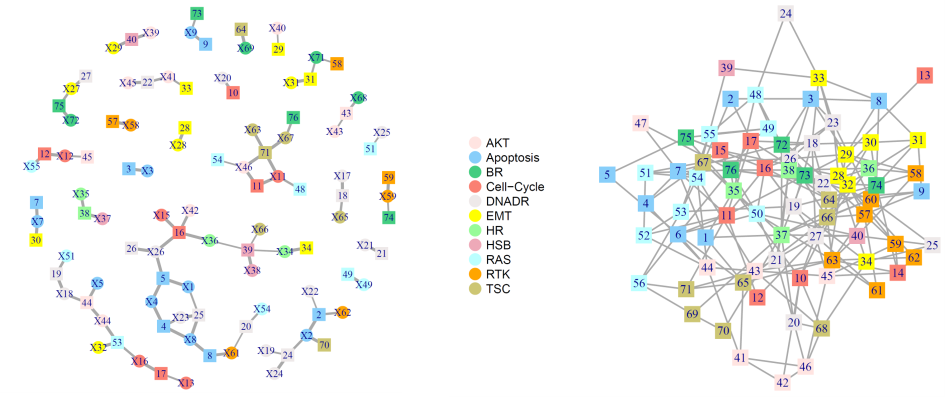
| Gene | Protein | Inclusion | |
|---|---|---|---|
| Probability | |||
| 1 | X2 | 2 | 1.00 |
| 2 | X22 | 2 | 0.50 |
| 3 | X62 | 2 | 0.74 |
| 4 | X3 | 3 | 0.98 |
| 5 | X4 | 4 | 1.00 |
| 6 | X8 | 4 | 1.00 |
| 7 | X23 | 4 | 0.80 |
| 8 | X1 | 5 | 1.00 |
| 9 | X4 | 5 | 1.00 |
| 10 | X26 | 5 | 0.98 |
| 11 | X7 | 7 | 1.00 |
| 12 | X8 | 8 | 1.00 |
| 13 | X61 | 8 | 0.92 |
| 14 | X9 | 9 | 0.93 |
| 15 | X20 | 10 | 0.89 |
| 16 | X11 | 11 | 1.00 |
| 17 | X46 | 11 | 0.99 |
| 18 | X12 | 12 | 1.00 |
| 19 | X55 | 12 | 1.00 |
| 20 | X15 | 16 | 1.00 |
| 21 | X26 | 16 | 1.00 |
| Gene | Protein | Inclusion | |
|---|---|---|---|
| Probability | |||
| 22 | X36 | 16 | 0.96 |
| 23 | X42 | 16 | 0.89 |
| 24 | X13 | 17 | 0.60 |
| 25 | X16 | 17 | 1.00 |
| 26 | X17 | 18 | 1.00 |
| 27 | X65 | 18 | 0.76 |
| 28 | X18 | 19 | 0.98 |
| 29 | X51 | 19 | 0.86 |
| 30 | X54 | 20 | 0.69 |
| 31 | X61 | 20 | 0.50 |
| 32 | X21 | 21 | 1.00 |
| 33 | X41 | 22 | 0.82 |
| 34 | X45 | 22 | 1.00 |
| 35 | X2 | 24 | 0.77 |
| 36 | X19 | 24 | 0.57 |
| 37 | X24 | 24 | 1.00 |
| 38 | X1 | 25 | 0.63 |
| 39 | X8 | 25 | 0.98 |
| 40 | X23 | 25 | 1.00 |
| 41 | X26 | 26 | 1.00 |
| 42 | X27 | 27 | 1.00 |
| Gene | Protein | Inclusion | |
|---|---|---|---|
| Probability | |||
| 43 | X28 | 28 | 1.00 |
| 44 | X40 | 29 | 0.51 |
| 45 | X7 | 30 | 1.00 |
| 46 | X31 | 31 | 1.00 |
| 47 | X71 | 31 | 0.66 |
| 48 | X41 | 33 | 0.64 |
| 49 | X34 | 34 | 1.00 |
| 50 | X35 | 38 | 0.92 |
| 51 | X37 | 38 | 1.00 |
| 52 | X34 | 39 | 0.51 |
| 53 | X36 | 39 | 0.52 |
| 54 | X38 | 39 | 1.00 |
| 55 | X66 | 39 | 0.52 |
| 56 | X29 | 40 | 0.98 |
| 57 | X39 | 40 | 0.97 |
| 58 | X43 | 43 | 0.58 |
| 59 | X68 | 43 | 0.80 |
| 60 | X5 | 44 | 0.94 |
| 61 | X18 | 44 | 0.84 |
| 62 | X44 | 44 | 0.97 |
| 63 | X12 | 45 | 0.62 |
| Gene | Protein | Inclusion | |
|---|---|---|---|
| Probability | |||
| 64 | X11 | 48 | 0.72 |
| 65 | X49 | 49 | 0.99 |
| 66 | X25 | 51 | 0.55 |
| 67 | X16 | 53 | 0.73 |
| 68 | X32 | 53 | 1.00 |
| 69 | X44 | 53 | 0.96 |
| 70 | X46 | 54 | 0.52 |
| 71 | X58 | 57 | 1.00 |
| 72 | X71 | 58 | 0.56 |
| 73 | X59 | 59 | 1.00 |
| 74 | X69 | 64 | 1.00 |
| 75 | X2 | 70 | 1.00 |
| 76 | X11 | 71 | 1.00 |
| 77 | X46 | 71 | 1.00 |
| 78 | X63 | 71 | 0.93 |
| 79 | X67 | 71 | 1.00 |
| 80 | X9 | 73 | 0.68 |
| 81 | X59 | 74 | 0.58 |
| 82 | X27 | 75 | 0.79 |
| 83 | X72 | 75 | 1.00 |
| 84 | X67 | 76 | 0.76 |
| Protein | Protein | Inclusion | |
|---|---|---|---|
| Probability | |||
| 1 | 2 | 3 | 1.00 |
| 2 | 5 | 6 | 1.00 |
| 3 | 1 | 7 | 1.00 |
| 4 | 4 | 7 | 1.00 |
| 5 | 3 | 8 | 1.00 |
| 6 | 6 | 11 | 1.00 |
| 7 | 7 | 11 | 1.00 |
| 8 | 11 | 12 | 1.00 |
| 9 | 4 | 15 | 1.00 |
| 10 | 2 | 16 | 1.00 |
| 11 | 11 | 16 | 1.00 |
| 12 | 11 | 17 | 1.00 |
| 13 | 17 | 18 | 1.00 |
| 14 | 16 | 19 | 1.00 |
| 15 | 18 | 19 | 1.00 |
| 16 | 10 | 20 | 1.00 |
| 17 | 20 | 21 | 1.00 |
| 18 | 18 | 22 | 1.00 |
| 19 | 3 | 23 | 1.00 |
| 20 | 16 | 23 | 0.97 |
| 21 | 16 | 26 | 1.00 |
| 22 | 23 | 26 | 1.00 |
| 23 | 12 | 27 | 1.00 |
| 24 | 16 | 27 | 1.00 |
| 25 | 18 | 27 | 1.00 |
| 26 | 15 | 28 | 1.00 |
| 27 | 22 | 28 | 0.67 |
| 28 | 23 | 28 | 1.00 |
| 29 | 3 | 29 | 1.00 |
| 30 | 8 | 29 | 1.00 |
| 31 | 11 | 29 | 1.00 |
| 32 | 13 | 29 | 1.00 |
| 33 | 26 | 29 | 1.00 |
| 34 | 28 | 30 | 1.00 |
| 35 | 8 | 31 | 1.00 |
| 36 | 9 | 31 | 1.00 |
| 37 | 30 | 31 | 1.00 |
| 38 | 10 | 32 | 1.00 |
| 39 | 22 | 32 | 1.00 |
| 40 | 31 | 32 | 1.00 |
| 41 | 8 | 33 | 1.00 |
| 42 | 18 | 33 | 1.00 |
| 43 | 23 | 33 | 1.00 |
| 44 | 24 | 33 | 1.00 |
| 45 | 32 | 33 | 1.00 |
| 46 | 19 | 34 | 1.00 |
| 47 | 25 | 34 | 1.00 |
| 48 | 28 | 34 | 1.00 |
| 49 | 1 | 35 | 1.00 |
| 50 | 10 | 35 | 1.00 |
| Protein | Protein | Inclusion | |
|---|---|---|---|
| Probability | |||
| 51 | 22 | 36 | 1.00 |
| 52 | 27 | 36 | 1.00 |
| 53 | 29 | 36 | 1.00 |
| 54 | 1 | 37 | 1.00 |
| 55 | 20 | 37 | 1.00 |
| 56 | 21 | 37 | 1.00 |
| 57 | 26 | 37 | 1.00 |
| 58 | 35 | 37 | 1.00 |
| 59 | 3 | 38 | 1.00 |
| 60 | 21 | 38 | 1.00 |
| 61 | 26 | 38 | 1.00 |
| 62 | 36 | 38 | 1.00 |
| 63 | 37 | 38 | 1.00 |
| 64 | 33 | 39 | 1.00 |
| 65 | 25 | 40 | 0.85 |
| 66 | 27 | 40 | 1.00 |
| 67 | 37 | 40 | 1.00 |
| 68 | 10 | 42 | 1.00 |
| 69 | 41 | 42 | 1.00 |
| 70 | 27 | 43 | 1.00 |
| 71 | 4 | 44 | 1.00 |
| 72 | 6 | 44 | 1.00 |
| 73 | 41 | 44 | 1.00 |
| 74 | 43 | 44 | 1.00 |
| 75 | 14 | 45 | 1.00 |
| 76 | 27 | 45 | 1.00 |
| 77 | 29 | 45 | 1.00 |
| 78 | 44 | 45 | 1.00 |
| 79 | 20 | 46 | 1.00 |
| 80 | 41 | 46 | 1.00 |
| 81 | 42 | 46 | 1.00 |
| 82 | 45 | 46 | 1.00 |
| 83 | 7 | 47 | 1.00 |
| 84 | 24 | 48 | 1.00 |
| 85 | 35 | 48 | 1.00 |
| 86 | 38 | 48 | 1.00 |
| 87 | 17 | 49 | 1.00 |
| 88 | 6 | 50 | 1.00 |
| 89 | 16 | 50 | 1.00 |
| 90 | 21 | 50 | 1.00 |
| 91 | 40 | 50 | 1.00 |
| 92 | 11 | 52 | 1.00 |
| 93 | 44 | 52 | 1.00 |
| 94 | 51 | 52 | 1.00 |
| 95 | 19 | 53 | 1.00 |
| 96 | 52 | 53 | 1.00 |
| 97 | 2 | 54 | 1.00 |
| 98 | 7 | 54 | 1.00 |
| 99 | 39 | 54 | 1.00 |
| 100 | 43 | 54 | 1.00 |
| Protein | Protein | Inclusion | |
|---|---|---|---|
| Probability | |||
| 101 | 44 | 54 | 1.00 |
| 102 | 51 | 54 | 1.00 |
| 103 | 53 | 54 | 1.00 |
| 104 | 48 | 55 | 1.00 |
| 105 | 49 | 55 | 1.00 |
| 106 | 50 | 55 | 1.00 |
| 107 | 53 | 55 | 1.00 |
| 108 | 6 | 56 | 1.00 |
| 109 | 53 | 56 | 1.00 |
| 110 | 9 | 57 | 1.00 |
| 111 | 32 | 57 | 1.00 |
| 112 | 49 | 57 | 1.00 |
| 113 | 29 | 58 | 1.00 |
| 114 | 36 | 58 | 1.00 |
| 115 | 40 | 58 | 1.00 |
| 116 | 14 | 59 | 1.00 |
| 117 | 28 | 59 | 1.00 |
| 118 | 45 | 59 | 1.00 |
| 119 | 57 | 59 | 1.00 |
| 120 | 9 | 60 | 1.00 |
| 121 | 23 | 60 | 1.00 |
| 122 | 25 | 60 | 1.00 |
| 123 | 37 | 60 | 1.00 |
| 124 | 57 | 60 | 1.00 |
| 125 | 27 | 61 | 1.00 |
| 126 | 57 | 61 | 1.00 |
| 127 | 14 | 62 | 1.00 |
| 128 | 32 | 62 | 1.00 |
| 129 | 14 | 63 | 1.00 |
| 130 | 22 | 63 | 1.00 |
| 131 | 40 | 63 | 1.00 |
| 132 | 43 | 63 | 1.00 |
| 133 | 50 | 63 | 1.00 |
| 134 | 57 | 63 | 1.00 |
| 135 | 61 | 63 | 1.00 |
| 136 | 62 | 63 | 1.00 |
| 137 | 9 | 64 | 1.00 |
| 138 | 10 | 64 | 1.00 |
| 139 | 16 | 64 | 1.00 |
| 140 | 38 | 64 | 1.00 |
| 141 | 1 | 65 | 1.00 |
| 142 | 6 | 65 | 1.00 |
| 143 | 41 | 65 | 1.00 |
| 144 | 63 | 65 | 0.92 |
| 145 | 26 | 66 | 1.00 |
| 146 | 30 | 66 | 0.91 |
| 147 | 57 | 66 | 1.00 |
| 148 | 60 | 66 | 1.00 |
| 149 | 65 | 66 | 1.00 |
| 150 | 26 | 67 | 1.00 |
| Protein | Protein | Inclusion | |
|---|---|---|---|
| Probability | |||
| 151 | 35 | 67 | 1.00 |
| 152 | 50 | 67 | 1.00 |
| 153 | 51 | 67 | 1.00 |
| 154 | 10 | 68 | 1.00 |
| 155 | 20 | 68 | 1.00 |
| 156 | 34 | 68 | 1.00 |
| 157 | 43 | 68 | 0.80 |
| 158 | 46 | 68 | 1.00 |
| 159 | 37 | 69 | 1.00 |
| 160 | 56 | 69 | 1.00 |
| 161 | 37 | 70 | 1.00 |
| 162 | 69 | 70 | 1.00 |
| 163 | 11 | 71 | 1.00 |
| 164 | 43 | 71 | 1.00 |
| 165 | 56 | 71 | 1.00 |
| 166 | 65 | 71 | 1.00 |
| 167 | 3 | 72 | 1.00 |
| 168 | 7 | 72 | 1.00 |
| 169 | 30 | 72 | 1.00 |
| 170 | 37 | 72 | 1.00 |
| 171 | 48 | 72 | 1.00 |
| 172 | 64 | 72 | 1.00 |
| 173 | 17 | 73 | 1.00 |
| 174 | 37 | 73 | 1.00 |
| 175 | 60 | 73 | 1.00 |
| 176 | 72 | 73 | 1.00 |
| 177 | 8 | 74 | 1.00 |
| 178 | 14 | 74 | 1.00 |
| 179 | 19 | 74 | 1.00 |
| 180 | 22 | 74 | 1.00 |
| 181 | 30 | 74 | 1.00 |
| 182 | 31 | 74 | 1.00 |
| 183 | 37 | 74 | 1.00 |
| 184 | 58 | 74 | 1.00 |
| 185 | 5 | 75 | 1.00 |
| 186 | 15 | 75 | 1.00 |
| 187 | 16 | 75 | 1.00 |
| 188 | 35 | 75 | 1.00 |
| 189 | 49 | 75 | 1.00 |
| 190 | 6 | 76 | 1.00 |
| 191 | 17 | 76 | 1.00 |
| 192 | 22 | 76 | 1.00 |
| 193 | 32 | 76 | 1.00 |
| 194 | 35 | 76 | 1.00 |
| 195 | 38 | 76 | 1.00 |
| 196 | 47 | 76 | 1.00 |
| 197 | 51 | 76 | 1.00 |
| Gene | Protein | |
|---|---|---|
| 1 | BAK1 | BAK |
| 2 | BAX | BAX |
| 3 | BID | BID |
| 4 | BCL2L11 | BIM |
| 5 | CASP7 | CASPASE7CLEAVEDD198 |
| 6 | BAD | BADPS112 |
| 7 | BCL2 | BCL2 |
| 8 | BCL2L1 | BCLXL |
| 9 | BIRC2 | CIAP |
| 10 | CDK1 | CDK1 |
| 11 | CCNB1 | CYCLINB1 |
| 12 | CCNE1 | CYCLINE1 |
| 13 | CCNE2 | CYCLINE2 |
| 14 | CDKN1B | P27PT157 |
| 15 | PCNA | P27PT198 |
| 16 | FOXM1 | PCNA |
| 17 | TP53BP1 | FOXM1 |
| 18 | ATM | 53BP1 |
| 19 | BRCA2 | ATM |
| 20 | CHEK1 | BRCA2 |
| 21 | CHEK2 | CHK1PS345 |
| 22 | XRCC5 | CHK2PT68 |
| 23 | MRE11A | KU80 |
| 24 | TP53 | MRE11 |
| 25 | RAD50 | P53 |
| 26 | RAD51 | RAD50 |
| 27 | XRCC1 | RAD51 |
| 28 | FN1 | XRCC1 |
| 29 | CDH2 | FIBRONECTIN |
| 30 | COL6A1 | NCADHERIN |
| 31 | CLDN7 | COLLAGENVI |
| 32 | CDH1 | CLAUDIN7 |
| 33 | CTNNB1 | ECADHERIN |
| 34 | SERPINE1 | BETACATENIN |
| 35 | ESR1 | PAI1 |
| 36 | PGR | ERALPHA |
| 37 | AR | ERALPHAPS118 |
| 38 | INPP4B | PR |
| 39 | GATA3 | AR |
| Gene | Protein | |
|---|---|---|
| 40 | AKT1 | INPP4B |
| 41 | AKT2 | GATA3 |
| 42 | AKT3 | AKTPS473 |
| 43 | GSK3A | AKTPT308 |
| 44 | GSK3B | GSK3ALPHABETAPS21S9 |
| 45 | AKT1S1 | GSK3PS9 |
| 46 | TSC2 | PRAS40PT246 |
| 47 | PTEN | TUBERINPT1462 |
| 48 | ARAF | PTEN |
| 49 | JUN | ARAFPS299 |
| 50 | RAF1 | CJUNPS73 |
| 51 | MAPK8 | CRAFPS338 |
| 52 | MAPK1 | JNKPT183Y185 |
| 53 | MAPK3 | MAPKPT202Y204 |
| 54 | MAP2K1 | MEK1PS217S221 |
| 55 | MAPK14 | P38PT180Y182 |
| 56 | RPS6KA1 | P90RSKPT359S363 |
| 57 | YBX1 | YB1PS102 |
| 58 | EGFR | EGFRPY1068 |
| 59 | ERBB2 | EGFRPY1173 |
| 60 | ERBB3 | HER2PY1248 |
| 61 | SHC1 | HER3PY1298 |
| 62 | SRC | SHCPY317 |
| 63 | EIF4EBP1 | SRCPY416 |
| 64 | RPS6KB1 | SRCPY527 |
| 65 | MTOR | 4EBP1PS65 |
| 66 | RPS6 | 4EBP1PT37T46 |
| 67 | RB1 | 4EBP1PT70 |
| 68 | CAV1 | P70S6KPT389 |
| 69 | MYH11 | MTORPS2448 |
| 70 | RAB11A | S6PS235S236 |
| 71 | RAB11B | S6PS240S244 |
| 72 | GAPDH | RBPS807S811 |
| 73 | RBM15 | CAVEOLIN1 |
| 74 | MYH11 | |
| 75 | RAB11 | |
| 76 | GAPDH | |
| 77 | RBM15 |
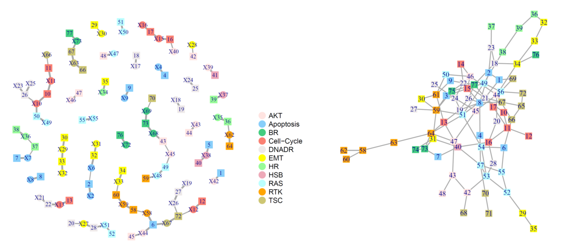
| Gene | Protein | Inclusion | |
|---|---|---|---|
| Probability | |||
| 1 | X42 | 1 | 0.94 |
| 2 | X2 | 2 | 1.00 |
| 3 | X6 | 2 | 0.50 |
| 4 | X4 | 4 | 1.00 |
| 5 | X38 | 5 | 0.98 |
| 6 | X44 | 6 | 1.00 |
| 7 | X58 | 6 | 1.00 |
| 8 | X67 | 6 | 0.95 |
| 9 | X7 | 7 | 1.00 |
| 10 | X8 | 8 | 1.00 |
| 11 | X9 | 9 | 1.00 |
| 12 | X10 | 10 | 1.00 |
| 13 | X11 | 10 | 1.00 |
| 14 | X11 | 11 | 1.00 |
| 15 | X66 | 11 | 0.54 |
| 16 | X12 | 12 | 1.00 |
| 17 | X13 | 13 | 1.00 |
| 18 | X15 | 16 | 1.00 |
| 19 | X40 | 16 | 0.60 |
| 20 | X15 | 17 | 0.95 |
| 21 | X16 | 17 | 1.00 |
| Gene | Protein | Inclusion | |
|---|---|---|---|
| Probability | |||
| 22 | X17 | 18 | 1.00 |
| 23 | X18 | 19 | 1.00 |
| 24 | X27 | 20 | 0.61 |
| 25 | X13 | 22 | 1.00 |
| 26 | X21 | 22 | 1.00 |
| 27 | X24 | 25 | 1.00 |
| 28 | X10 | 26 | 0.60 |
| 29 | X23 | 26 | 1.00 |
| 30 | X25 | 26 | 1.00 |
| 31 | X19 | 27 | 0.99 |
| 32 | X26 | 27 | 1.00 |
| 33 | X27 | 28 | 1.00 |
| 34 | X51 | 28 | 0.93 |
| 35 | X30 | 29 | 0.55 |
| 36 | X29 | 30 | 1.00 |
| 37 | X6 | 32 | 1.00 |
| 38 | X31 | 32 | 1.00 |
| 39 | X29 | 33 | 1.00 |
| 40 | X32 | 33 | 1.00 |
| 41 | X33 | 34 | 1.00 |
| 42 | X34 | 35 | 1.00 |
| Gene | Protein | Inclusion | |
|---|---|---|---|
| Probability | |||
| 43 | X35 | 36 | 1.00 |
| 44 | X62 | 36 | 0.62 |
| 45 | X7 | 37 | 0.50 |
| 46 | X36 | 37 | 0.57 |
| 47 | X36 | 38 | 1.00 |
| 48 | X37 | 39 | 1.00 |
| 49 | X38 | 40 | 1.00 |
| 50 | X39 | 41 | 1.00 |
| 51 | X28 | 42 | 0.57 |
| 52 | X45 | 43 | 0.50 |
| 53 | X68 | 43 | 0.91 |
| 54 | X43 | 44 | 1.00 |
| 55 | X44 | 45 | 0.84 |
| 56 | X46 | 47 | 1.00 |
| 57 | X47 | 48 | 1.00 |
| 58 | X45 | 49 | 0.59 |
| 59 | X48 | 49 | 1.00 |
| 60 | X10 | 50 | 0.94 |
| 61 | X49 | 50 | 1.00 |
| 62 | X50 | 51 | 1.00 |
| 63 | X51 | 52 | 0.90 |
| Gene | Protein | Inclusion | |
|---|---|---|---|
| Probability | |||
| 64 | X55 | 55 | 1.00 |
| 65 | X58 | 58 | 0.52 |
| 66 | X59 | 58 | 1.00 |
| 67 | X48 | 59 | 0.83 |
| 68 | X33 | 60 | 0.60 |
| 69 | X59 | 60 | 1.00 |
| 70 | X62 | 64 | 0.99 |
| 71 | X63 | 66 | 1.00 |
| 72 | X63 | 67 | 1.00 |
| 73 | X73 | 67 | 0.88 |
| 74 | X69 | 70 | 0.53 |
| 75 | X12 | 72 | 0.52 |
| 76 | X26 | 72 | 0.59 |
| 77 | X67 | 72 | 0.98 |
| 78 | X68 | 73 | 1.00 |
| 79 | X69 | 73 | 1.00 |
| 80 | X72 | 76 | 1.00 |
| 81 | X73 | 77 | 1.00 |
| Gene | Protein | Inclusion | |
|---|---|---|---|
| Probability | |||
| 1 | 1 | 2 | 1.00 |
| 2 | 2 | 8 | 1.00 |
| 3 | 4 | 8 | 1.00 |
| 4 | 10 | 11 | 1.00 |
| 5 | 11 | 12 | 1.00 |
| 6 | 3 | 15 | 1.00 |
| 7 | 8 | 15 | 1.00 |
| 8 | 11 | 16 | 1.00 |
| 9 | 11 | 17 | 1.00 |
| 10 | 8 | 19 | 1.00 |
| 11 | 13 | 19 | 1.00 |
| 12 | 16 | 20 | 1.00 |
| 13 | 1 | 21 | 1.00 |
| 14 | 10 | 21 | 1.00 |
| 15 | 14 | 22 | 1.00 |
| 16 | 21 | 22 | 1.00 |
| 17 | 2 | 23 | 1.00 |
| 18 | 18 | 23 | 1.00 |
| 19 | 3 | 24 | 1.00 |
| 20 | 22 | 24 | 1.00 |
| 21 | 24 | 25 | 1.00 |
| 22 | 8 | 26 | 1.00 |
| 23 | 19 | 26 | 1.00 |
| 24 | 16 | 28 | 1.00 |
| 25 | 32 | 33 | 1.00 |
| 26 | 18 | 34 | 1.00 |
| 27 | 33 | 34 | 1.00 |
| 28 | 29 | 35 | 1.00 |
| Gene | Protein | Inclusion | |
|---|---|---|---|
| Probability | |||
| 29 | 32 | 36 | 1.00 |
| 30 | 23 | 37 | 1.00 |
| 31 | 36 | 39 | 1.00 |
| 32 | 38 | 39 | 1.00 |
| 33 | 7 | 40 | 1.00 |
| 34 | 13 | 40 | 1.00 |
| 35 | 16 | 40 | 1.00 |
| 36 | 31 | 40 | 1.00 |
| 37 | 42 | 43 | 1.00 |
| 38 | 20 | 44 | 1.00 |
| 39 | 34 | 44 | 1.00 |
| 40 | 24 | 45 | 1.00 |
| 41 | 44 | 45 | 1.00 |
| 42 | 14 | 46 | 1.00 |
| 43 | 15 | 46 | 1.00 |
| 44 | 44 | 46 | 1.00 |
| 45 | 43 | 47 | 1.00 |
| 46 | 45 | 47 | 1.00 |
| 47 | 43 | 48 | 1.00 |
| 48 | 15 | 49 | 1.00 |
| 49 | 38 | 49 | 1.00 |
| 50 | 46 | 50 | 1.00 |
| 51 | 21 | 51 | 1.00 |
| 52 | 24 | 51 | 1.00 |
| 53 | 49 | 51 | 1.00 |
| 54 | 29 | 52 | 1.00 |
| 55 | 28 | 53 | 1.00 |
| 56 | 42 | 53 | 1.00 |
| Gene | Protein | Inclusion | |
|---|---|---|---|
| Probability | |||
| 57 | 52 | 53 | 1.00 |
| 58 | 6 | 54 | 1.00 |
| 59 | 51 | 54 | 1.00 |
| 60 | 53 | 54 | 1.00 |
| 61 | 6 | 55 | 1.00 |
| 62 | 52 | 55 | 1.00 |
| 63 | 45 | 56 | 1.00 |
| 64 | 49 | 56 | 1.00 |
| 65 | 4 | 57 | 1.00 |
| 66 | 40 | 57 | 1.00 |
| 67 | 53 | 57 | 1.00 |
| 68 | 55 | 57 | 1.00 |
| 69 | 3 | 59 | 1.00 |
| 70 | 27 | 59 | 1.00 |
| 71 | 30 | 59 | 1.00 |
| 72 | 31 | 59 | 1.00 |
| 73 | 51 | 59 | 1.00 |
| 74 | 58 | 60 | 1.00 |
| 75 | 9 | 61 | 1.00 |
| 76 | 13 | 61 | 1.00 |
| 77 | 30 | 61 | 1.00 |
| 78 | 50 | 61 | 1.00 |
| 79 | 58 | 62 | 1.00 |
| 80 | 58 | 63 | 1.00 |
| 81 | 13 | 64 | 1.00 |
| 82 | 47 | 64 | 1.00 |
| 83 | 51 | 64 | 1.00 |
| 84 | 63 | 64 | 1.00 |
| Gene | Protein | Inclusion | |
|---|---|---|---|
| Probability | |||
| 85 | 6 | 66 | 1.00 |
| 86 | 44 | 66 | 1.00 |
| 87 | 65 | 66 | 1.00 |
| 88 | 8 | 67 | 1.00 |
| 89 | 21 | 67 | 1.00 |
| 90 | 65 | 67 | 1.00 |
| 91 | 42 | 68 | 1.00 |
| 92 | 1 | 69 | 1.00 |
| 93 | 56 | 69 | 1.00 |
| 94 | 57 | 70 | 1.00 |
| 95 | 70 | 71 | 1.00 |
| 96 | 56 | 72 | 1.00 |
| 97 | 65 | 72 | 1.00 |
| 98 | 7 | 73 | 1.00 |
| 99 | 31 | 73 | 1.00 |
| 100 | 64 | 73 | 1.00 |
| 101 | 31 | 74 | 1.00 |
| 102 | 73 | 74 | 1.00 |
| 103 | 3 | 75 | 1.00 |
| 104 | 22 | 75 | 1.00 |
| 105 | 59 | 75 | 0.78 |
| 106 | 34 | 76 | 1.00 |
| 107 | 9 | 77 | 1.00 |
| 108 | 17 | 77 | 1.00 |
| 109 | 18 | 77 | 1.00 |
| 110 | 26 | 77 | 1.00 |
| 111 | 75 | 77 | 1.00 |
| Gene | Protein | |
|---|---|---|
| 1 | BAK1 | BAK |
| 2 | BAX | BAX |
| 3 | BID | BID |
| 4 | BCL2L11 | BIM |
| 5 | CASP7 | CASPASE7CLEAVEDD198 |
| 6 | BAD | BADPS112 |
| 7 | BCL2 | BCL2 |
| 8 | BCL2L1 | BCLXL |
| 9 | BIRC2 | CIAP |
| 10 | CDK1 | CDK1 |
| 11 | CCNB1 | CYCLINB1 |
| 12 | CCNE1 | CYCLINE1 |
| 13 | CCNE2 | CYCLINE2 |
| 14 | CDKN1B | P27PT157 |
| 15 | PCNA | P27PT198 |
| 16 | FOXM1 | PCNA |
| 17 | TP53BP1 | FOXM1 |
| 18 | ATM | 53BP1 |
| 19 | BRCA2 | ATM |
| 20 | CHEK1 | CHK1PS345 |
| 21 | CHEK2 | CHK2PT68 |
| 22 | XRCC5 | KU80 |
| 23 | MRE11A | MRE11 |
| 24 | TP53 | P53 |
| 25 | RAD50 | RAD50 |
| 26 | RAD51 | RAD51 |
| 27 | XRCC1 | XRCC1 |
| 28 | FN1 | FIBRONECTIN |
| 29 | CDH2 | NCADHERIN |
| 30 | COL6A1 | COLLAGENVI |
| 31 | CLDN7 | CLAUDIN7 |
| 32 | CDH1 | ECADHERIN |
| 33 | CTNNB1 | BETACATENIN |
| 34 | SERPINE1 | PAI1 |
| 35 | ESR1 | ERALPHA |
| 36 | PGR | ERALPHAPS118 |
| 37 | AR | PR |
| 38 | INPP4B | AR |
| Gene | Protein | |
|---|---|---|
| 39 | GATA3 | INPP4B |
| 40 | AKT1 | GATA3 |
| 41 | AKT2 | AKTPS473 |
| 42 | AKT3 | AKTPT308 |
| 43 | GSK3A | GSK3ALPHABETAPS21S9 |
| 44 | GSK3B | GSK3PS9 |
| 45 | AKT1S1 | PRAS40PT246 |
| 46 | TSC2 | TUBERINPT1462 |
| 47 | PTEN | PTEN |
| 48 | ARAF | ARAFPS299 |
| 49 | JUN | CJUNPS73 |
| 50 | RAF1 | CRAFPS338 |
| 51 | MAPK8 | JNKPT183Y185 |
| 52 | MAPK1 | MAPKPT202Y204 |
| 53 | MAPK3 | MEK1PS217S221 |
| 54 | MAP2K1 | P38PT180Y182 |
| 55 | MAPK14 | P90RSKPT359S363 |
| 56 | RPS6KA1 | YB1PS102 |
| 57 | YBX1 | EGFRPY1068 |
| 58 | EGFR | EGFRPY1173 |
| 59 | ERBB2 | HER2PY1248 |
| 60 | ERBB3 | HER3PY1298 |
| 61 | SHC1 | SHCPY317 |
| 62 | SRC | SRCPY416 |
| 63 | EIF4EBP1 | SRCPY527 |
| 64 | RPS6KB1 | 4EBP1PS65 |
| 65 | MTOR | 4EBP1PT37T46 |
| 66 | RPS6 | 4EBP1PT70 |
| 67 | RB1 | P70S6KPT389 |
| 68 | CAV1 | MTORPS2448 |
| 69 | MYH11 | S6PS235S236 |
| 70 | RAB11A | S6PS240S244 |
| 71 | RAB11B | RBPS807S811 |
| 72 | GAPDH | CAVEOLIN1 |
| 73 | RBM15 | MYH11 |
| 74 | RAB11 | |
| 75 | GAPDH | |
| 76 | RBM15 |
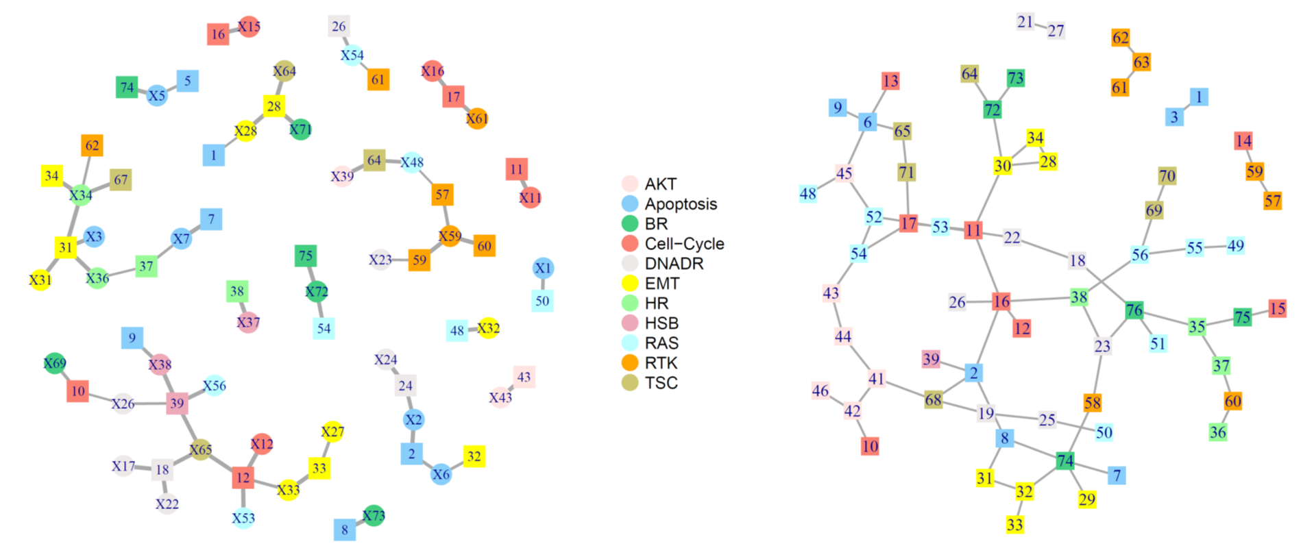
| Gene | Protein | Inclusion | |
|---|---|---|---|
| Probability | |||
| 1 | X28 | 1 | 0.54 |
| 2 | X2 | 2 | 1.00 |
| 3 | X6 | 2 | 0.76 |
| 4 | X5 | 5 | 0.68 |
| 5 | X7 | 7 | 1.00 |
| 6 | X73 | 8 | 1.00 |
| 7 | X38 | 9 | 0.83 |
| 8 | X26 | 10 | 0.54 |
| 9 | X69 | 10 | 0.75 |
| 10 | X11 | 11 | 1.00 |
| 11 | X12 | 12 | 1.00 |
| 12 | X33 | 12 | 0.72 |
| 13 | X53 | 12 | 1.00 |
| 14 | X65 | 12 | 0.96 |
| 15 | X15 | 16 | 1.00 |
| Gene | Protein | Inclusion | |
|---|---|---|---|
| Probability | |||
| 16 | X16 | 17 | 0.97 |
| 17 | X61 | 17 | 0.98 |
| 18 | X17 | 18 | 1.00 |
| 19 | X22 | 18 | 0.98 |
| 20 | X65 | 18 | 0.94 |
| 21 | X2 | 24 | 0.91 |
| 22 | X24 | 24 | 1.00 |
| 23 | X54 | 26 | 0.82 |
| 24 | X28 | 28 | 1.00 |
| 25 | X64 | 28 | 1.00 |
| 26 | X71 | 28 | 1.00 |
| 27 | X3 | 31 | 0.97 |
| 28 | X31 | 31 | 1.00 |
| 29 | X34 | 31 | 0.99 |
| 30 | X36 | 31 | 0.99 |
| Gene | Protein | Inclusion | |
|---|---|---|---|
| Probability | |||
| 31 | X6 | 32 | 0.67 |
| 32 | X27 | 33 | 0.73 |
| 33 | X33 | 33 | 1.00 |
| 34 | X34 | 34 | 1.00 |
| 35 | X7 | 37 | 0.65 |
| 36 | X36 | 37 | 0.57 |
| 37 | X37 | 38 | 1.00 |
| 38 | X26 | 39 | 0.63 |
| 39 | X38 | 39 | 1.00 |
| 40 | X56 | 39 | 0.94 |
| 41 | X65 | 39 | 0.93 |
| 42 | X43 | 43 | 1.00 |
| 43 | X32 | 48 | 0.97 |
| 44 | X1 | 50 | 0.84 |
| 45 | X72 | 54 | 0.94 |
| Gene | Protein | Inclusion | |
|---|---|---|---|
| Probability | |||
| 46 | X48 | 57 | 0.52 |
| 47 | X59 | 57 | 0.78 |
| 48 | X23 | 59 | 0.60 |
| 49 | X59 | 59 | 1.00 |
| 50 | X59 | 60 | 1.00 |
| 51 | X54 | 61 | 0.52 |
| 52 | X34 | 62 | 0.61 |
| 53 | X39 | 64 | 0.97 |
| 54 | X48 | 64 | 0.88 |
| 55 | X34 | 67 | 0.92 |
| 56 | X5 | 74 | 0.97 |
| 57 | X72 | 75 | 1.00 |
| Protein | Protein | Inclusion | |
|---|---|---|---|
| Probability | |||
| 1 | 1 | 3 | 1.00 |
| 2 | 2 | 8 | 1.00 |
| 3 | 6 | 9 | 1.00 |
| 4 | 6 | 13 | 1.00 |
| 5 | 2 | 16 | 1.00 |
| 6 | 11 | 16 | 1.00 |
| 7 | 12 | 16 | 1.00 |
| 8 | 11 | 17 | 1.00 |
| 9 | 18 | 22 | 1.00 |
| 10 | 19 | 25 | 1.00 |
| 11 | 16 | 26 | 1.00 |
| 12 | 21 | 27 | 1.00 |
| 13 | 11 | 30 | 1.00 |
| 14 | 28 | 30 | 1.00 |
| 15 | 8 | 31 | 1.00 |
| 16 | 31 | 32 | 1.00 |
| 17 | 32 | 33 | 1.00 |
| 18 | 28 | 34 | 1.00 |
| Protein | Protein | Inclusion | |
|---|---|---|---|
| Probability | |||
| 19 | 30 | 34 | 1.00 |
| 20 | 35 | 37 | 1.00 |
| 21 | 16 | 38 | 1.00 |
| 22 | 23 | 38 | 1.00 |
| 23 | 2 | 39 | 1.00 |
| 24 | 10 | 42 | 1.00 |
| 25 | 41 | 42 | 1.00 |
| 26 | 41 | 44 | 1.00 |
| 27 | 43 | 44 | 1.00 |
| 28 | 6 | 45 | 1.00 |
| 29 | 42 | 46 | 1.00 |
| 30 | 45 | 48 | 1.00 |
| 31 | 25 | 50 | 1.00 |
| 32 | 45 | 52 | 1.00 |
| 33 | 22 | 53 | 1.00 |
| 34 | 52 | 53 | 1.00 |
| 35 | 17 | 54 | 1.00 |
| 36 | 43 | 54 | 1.00 |
| Protein | Protein | Inclusion | |
|---|---|---|---|
| Probability | |||
| 37 | 52 | 54 | 1.00 |
| 38 | 49 | 55 | 1.00 |
| 39 | 38 | 56 | 1.00 |
| 40 | 55 | 56 | 1.00 |
| 41 | 23 | 58 | 1.00 |
| 42 | 14 | 59 | 1.00 |
| 43 | 57 | 59 | 1.00 |
| 44 | 36 | 60 | 1.00 |
| 45 | 37 | 60 | 1.00 |
| 46 | 61 | 63 | 1.00 |
| 47 | 62 | 63 | 1.00 |
| 48 | 6 | 65 | 1.00 |
| 49 | 2 | 68 | 1.00 |
| 50 | 19 | 68 | 1.00 |
| 51 | 41 | 68 | 1.00 |
| 52 | 56 | 69 | 1.00 |
| 53 | 69 | 70 | 1.00 |
| 54 | 17 | 71 | 1.00 |
| Protein | Protein | Inclusion | |
|---|---|---|---|
| Probability | |||
| 55 | 65 | 71 | 1.00 |
| 56 | 30 | 72 | 1.00 |
| 57 | 64 | 72 | 1.00 |
| 58 | 72 | 73 | 1.00 |
| 59 | 7 | 74 | 1.00 |
| 60 | 8 | 74 | 1.00 |
| 61 | 29 | 74 | 1.00 |
| 62 | 32 | 74 | 1.00 |
| 63 | 58 | 74 | 0.95 |
| 64 | 15 | 75 | 1.00 |
| 65 | 35 | 75 | 1.00 |
| 66 | 18 | 76 | 1.00 |
| 67 | 23 | 76 | 1.00 |
| 68 | 35 | 76 | 1.00 |
| 69 | 51 | 76 | 1.00 |
| Gene | Protein | |
|---|---|---|
| 1 | BAK1 | BAK |
| 2 | BAX | BAX |
| 3 | BID | BID |
| 4 | BCL2L11 | BIM |
| 5 | CASP7 | CASPASE7CLEAVEDD198 |
| 6 | BAD | BADPS112 |
| 7 | BCL2 | BCL2 |
| 8 | BCL2L1 | BCLXL |
| 9 | BIRC2 | CIAP |
| 10 | CDK1 | CDK1 |
| 11 | CCNB1 | CYCLINB1 |
| 12 | CCNE1 | CYCLINE1 |
| 13 | CCNE2 | CYCLINE2 |
| 14 | CDKN1B | P27PT157 |
| 15 | PCNA | P27PT198 |
| 16 | FOXM1 | PCNA |
| 17 | TP53BP1 | FOXM1 |
| 18 | ATM | 53BP1 |
| 19 | BRCA2 | ATM |
| 20 | CHEK1 | CHK1PS345 |
| 21 | CHEK2 | CHK2PT68 |
| 22 | XRCC5 | KU80 |
| 23 | MRE11A | MRE11 |
| 24 | TP53 | P53 |
| 25 | RAD50 | RAD50 |
| 26 | RAD51 | RAD51 |
| 27 | XRCC1 | XRCC1 |
| 28 | FN1 | FIBRONECTIN |
| 29 | CDH2 | NCADHERIN |
| 30 | COL6A1 | COLLAGENVI |
| 31 | CLDN7 | CLAUDIN7 |
| 32 | CDH1 | ECADHERIN |
| 33 | CTNNB1 | BETACATENIN |
| 34 | SERPINE1 | PAI1 |
| 35 | ESR1 | ERALPHA |
| 36 | PGR | ERALPHAPS118 |
| 37 | AR | PR |
| 38 | INPP4B | AR |
| Gene | Protein | |
|---|---|---|
| 39 | GATA3 | INPP4B |
| 40 | AKT1 | GATA3 |
| 41 | AKT2 | AKTPS473 |
| 42 | AKT3 | AKTPT308 |
| 43 | GSK3A | GSK3ALPHABETAPS21S9 |
| 44 | GSK3B | GSK3PS9 |
| 45 | AKT1S1 | PRAS40PT246 |
| 46 | TSC2 | TUBERINPT1462 |
| 47 | PTEN | PTEN |
| 48 | ARAF | ARAFPS299 |
| 49 | JUN | CJUNPS73 |
| 50 | RAF1 | CRAFPS338 |
| 51 | MAPK8 | JNKPT183Y185 |
| 52 | MAPK1 | MAPKPT202Y204 |
| 53 | MAPK3 | MEK1PS217S221 |
| 54 | MAP2K1 | P38PT180Y182 |
| 55 | MAPK14 | P90RSKPT359S363 |
| 56 | RPS6KA1 | YB1PS102 |
| 57 | YBX1 | EGFRPY1068 |
| 58 | EGFR | EGFRPY1173 |
| 59 | ERBB2 | HER2PY1248 |
| 60 | ERBB3 | HER3PY1298 |
| 61 | SHC1 | SHCPY317 |
| 62 | SRC | SRCPY416 |
| 63 | EIF4EBP1 | SRCPY527 |
| 64 | RPS6KB1 | 4EBP1PS65 |
| 65 | MTOR | 4EBP1PT37T46 |
| 66 | RPS6 | 4EBP1PT70 |
| 67 | RB1 | P70S6KPT389 |
| 68 | CAV1 | MTORPS2448 |
| 69 | MYH11 | S6PS235S236 |
| 70 | RAB11A | S6PS240S244 |
| 71 | RAB11B | RBPS807S811 |
| 72 | GAPDH | CAVEOLIN1 |
| 73 | RBM15 | MYH11 |
| 74 | 1 | RAB11 |
| 75 | 2 | GAPDH |
| 76 | 3 | RBM15 |
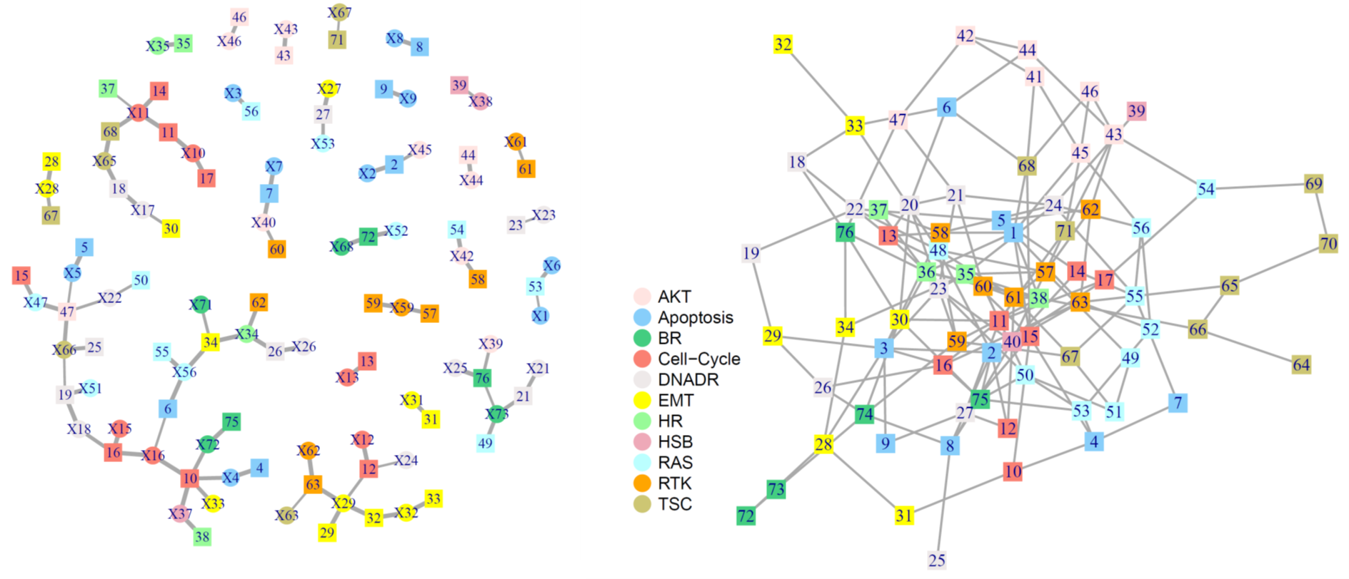
| Gene | Protein | Inclusion | |
|---|---|---|---|
| Probability | |||
| 1 | X2 | 2 | 1.00 |
| 2 | X45 | 2 | 0.73 |
| 3 | X4 | 4 | 1.00 |
| 4 | X5 | 5 | 1.00 |
| 5 | X16 | 6 | 0.56 |
| 6 | X56 | 6 | 0.97 |
| 7 | X7 | 7 | 1.00 |
| 8 | X40 | 7 | 0.96 |
| 9 | X8 | 8 | 1.00 |
| 10 | X9 | 9 | 1.00 |
| 11 | X4 | 10 | 0.89 |
| 12 | X16 | 10 | 0.98 |
| 13 | X33 | 10 | 0.88 |
| 14 | X37 | 10 | 1.00 |
| 15 | X72 | 10 | 0.86 |
| 16 | X10 | 11 | 1.00 |
| 17 | X11 | 11 | 1.00 |
| 18 | X12 | 12 | 1.00 |
| 19 | X24 | 12 | 0.53 |
| 20 | X29 | 12 | 0.65 |
| 21 | X13 | 13 | 1.00 |
| 22 | X11 | 14 | 1.00 |
| Gene | Protein | Inclusion | |
|---|---|---|---|
| Probability | |||
| 23 | X47 | 15 | 0.90 |
| 24 | X15 | 16 | 1.00 |
| 25 | X16 | 16 | 1.00 |
| 26 | X18 | 16 | 0.84 |
| 27 | X10 | 17 | 1.00 |
| 28 | X17 | 18 | 1.00 |
| 29 | X65 | 18 | 0.98 |
| 30 | X18 | 19 | 1.00 |
| 31 | X51 | 19 | 0.99 |
| 32 | X66 | 19 | 0.55 |
| 33 | X21 | 21 | 0.88 |
| 34 | X73 | 21 | 0.86 |
| 35 | X23 | 23 | 0.53 |
| 36 | X66 | 25 | 0.90 |
| 37 | X26 | 26 | 1.00 |
| 38 | X34 | 26 | 0.98 |
| 39 | X27 | 27 | 1.00 |
| 40 | X53 | 27 | 0.79 |
| 41 | X28 | 28 | 1.00 |
| 42 | X29 | 29 | 1.00 |
| 43 | X17 | 30 | 0.66 |
| 44 | X31 | 31 | 1.00 |
| Gene | Protein | Inclusion | |
|---|---|---|---|
| Probability | |||
| 45 | X29 | 32 | 1.00 |
| 46 | X32 | 32 | 1.00 |
| 47 | X32 | 33 | 1.00 |
| 48 | X34 | 34 | 1.00 |
| 49 | X56 | 34 | 0.99 |
| 50 | X71 | 34 | 0.69 |
| 51 | X35 | 35 | 1.00 |
| 52 | X11 | 37 | 0.52 |
| 53 | X37 | 38 | 1.00 |
| 54 | X38 | 39 | 0.68 |
| 55 | X43 | 43 | 1.00 |
| 56 | X44 | 44 | 1.00 |
| 57 | X46 | 46 | 0.87 |
| 58 | X5 | 47 | 0.53 |
| 59 | X22 | 47 | 0.64 |
| 60 | X47 | 47 | 1.00 |
| 61 | X66 | 47 | 0.91 |
| 62 | X73 | 49 | 0.91 |
| 63 | X22 | 50 | 0.62 |
| 64 | X1 | 53 | 0.52 |
| 65 | X6 | 53 | 0.93 |
| 66 | X42 | 54 | 0.98 |
| Gene | Protein | Inclusion | |
|---|---|---|---|
| Probability | |||
| 67 | X56 | 55 | 1.00 |
| 68 | X3 | 56 | 0.98 |
| 69 | X59 | 57 | 0.92 |
| 70 | X42 | 58 | 0.90 |
| 71 | X59 | 59 | 1.00 |
| 72 | X40 | 60 | 0.73 |
| 73 | X61 | 61 | 0.63 |
| 74 | X34 | 62 | 0.91 |
| 75 | X29 | 63 | 0.99 |
| 76 | X62 | 63 | 1.00 |
| 77 | X63 | 63 | 0.52 |
| 78 | X28 | 67 | 0.79 |
| 79 | X11 | 68 | 0.93 |
| 80 | X65 | 68 | 1.00 |
| 81 | X67 | 71 | 0.51 |
| 82 | X52 | 72 | 1.00 |
| 83 | X68 | 72 | 1.00 |
| 84 | X72 | 75 | 1.00 |
| 85 | X25 | 76 | 1.00 |
| 86 | X39 | 76 | 0.72 |
| 87 | X73 | 76 | 0.58 |
| Protein | Protein | Inclusion | |
|---|---|---|---|
| Probability | |||
| 1 | 2 | 3 | 1.00 |
| 2 | 4 | 7 | 1.00 |
| 3 | 2 | 8 | 1.00 |
| 4 | 3 | 9 | 1.00 |
| 5 | 4 | 10 | 1.00 |
| 6 | 2 | 12 | 1.00 |
| 7 | 5 | 14 | 1.00 |
| 8 | 1 | 15 | 1.00 |
| 9 | 4 | 15 | 1.00 |
| 10 | 10 | 15 | 1.00 |
| 11 | 3 | 16 | 1.00 |
| 12 | 11 | 16 | 1.00 |
| 13 | 2 | 17 | 1.00 |
| 14 | 11 | 17 | 1.00 |
| 15 | 6 | 20 | 1.00 |
| 16 | 13 | 20 | 1.00 |
| 17 | 20 | 21 | 1.00 |
| 18 | 5 | 22 | 1.00 |
| 19 | 13 | 22 | 1.00 |
| 20 | 18 | 22 | 1.00 |
| 21 | 19 | 22 | 1.00 |
| 22 | 3 | 23 | 1.00 |
| 23 | 20 | 23 | 1.00 |
| 24 | 21 | 23 | 1.00 |
| 25 | 21 | 24 | 1.00 |
| 26 | 8 | 25 | 1.00 |
| 27 | 16 | 26 | 1.00 |
| 28 | 9 | 27 | 1.00 |
| 29 | 11 | 27 | 1.00 |
| 30 | 12 | 27 | 1.00 |
| 31 | 15 | 27 | 1.00 |
| 32 | 3 | 28 | 1.00 |
| 33 | 3 | 29 | 1.00 |
| 34 | 19 | 29 | 1.00 |
| 35 | 26 | 29 | 1.00 |
| 36 | 11 | 30 | 1.00 |
| 37 | 20 | 30 | 1.00 |
| 38 | 10 | 31 | 1.00 |
| 39 | 28 | 31 | 1.00 |
| Protein | Protein | Inclusion | |
|---|---|---|---|
| Probability | |||
| 40 | 6 | 33 | 1.00 |
| 41 | 18 | 33 | 1.00 |
| 42 | 32 | 33 | 1.00 |
| 43 | 28 | 34 | 1.00 |
| 44 | 13 | 35 | 1.00 |
| 45 | 15 | 35 | 1.00 |
| 46 | 23 | 35 | 1.00 |
| 47 | 24 | 35 | 1.00 |
| 48 | 34 | 35 | 0.76 |
| 49 | 1 | 36 | 1.00 |
| 50 | 3 | 36 | 1.00 |
| 51 | 13 | 36 | 1.00 |
| 52 | 23 | 37 | 1.00 |
| 53 | 1 | 38 | 1.00 |
| 54 | 35 | 38 | 1.00 |
| 55 | 36 | 38 | 1.00 |
| 56 | 24 | 39 | 1.00 |
| 57 | 8 | 40 | 1.00 |
| 58 | 12 | 40 | 1.00 |
| 59 | 14 | 40 | 1.00 |
| 60 | 23 | 40 | 1.00 |
| 61 | 41 | 42 | 1.00 |
| 62 | 6 | 44 | 1.00 |
| 63 | 42 | 44 | 1.00 |
| 64 | 43 | 44 | 1.00 |
| 65 | 1 | 45 | 1.00 |
| 66 | 41 | 45 | 1.00 |
| 67 | 43 | 46 | 1.00 |
| 68 | 45 | 46 | 1.00 |
| 69 | 21 | 47 | 1.00 |
| 70 | 42 | 47 | 1.00 |
| 71 | 2 | 48 | 1.00 |
| 72 | 22 | 48 | 1.00 |
| 73 | 33 | 48 | 1.00 |
| 74 | 23 | 50 | 1.00 |
| 75 | 49 | 51 | 1.00 |
| 76 | 50 | 51 | 1.00 |
| 77 | 4 | 53 | 1.00 |
| 78 | 50 | 53 | 1.00 |
| Protein | Protein | Inclusion | |
|---|---|---|---|
| Probability | |||
| 79 | 52 | 53 | 1.00 |
| 80 | 17 | 54 | 1.00 |
| 81 | 43 | 54 | 1.00 |
| 82 | 7 | 55 | 1.00 |
| 83 | 14 | 55 | 1.00 |
| 84 | 24 | 55 | 1.00 |
| 85 | 24 | 56 | 1.00 |
| 86 | 45 | 56 | 1.00 |
| 87 | 52 | 56 | 1.00 |
| 88 | 55 | 56 | 1.00 |
| 89 | 35 | 57 | 1.00 |
| 90 | 48 | 57 | 1.00 |
| 91 | 49 | 57 | 1.00 |
| 92 | 1 | 58 | 1.00 |
| 93 | 3 | 58 | 1.00 |
| 94 | 13 | 58 | 1.00 |
| 95 | 24 | 58 | 1.00 |
| 96 | 37 | 58 | 1.00 |
| 97 | 23 | 59 | 1.00 |
| 98 | 38 | 59 | 1.00 |
| 99 | 48 | 59 | 1.00 |
| 100 | 21 | 60 | 1.00 |
| 101 | 36 | 60 | 1.00 |
| 102 | 38 | 60 | 1.00 |
| 103 | 50 | 60 | 1.00 |
| 104 | 38 | 61 | 1.00 |
| 105 | 40 | 61 | 1.00 |
| 106 | 48 | 61 | 1.00 |
| 107 | 57 | 61 | 1.00 |
| 108 | 60 | 61 | 1.00 |
| 109 | 5 | 62 | 1.00 |
| 110 | 43 | 62 | 1.00 |
| 111 | 57 | 62 | 1.00 |
| 112 | 2 | 63 | 1.00 |
| 113 | 5 | 63 | 1.00 |
| 114 | 16 | 63 | 1.00 |
| 115 | 52 | 63 | 1.00 |
| 116 | 62 | 63 | 1.00 |
| 117 | 63 | 65 | 1.00 |
| Protein | Protein | Inclusion | |
|---|---|---|---|
| Probability | |||
| 118 | 38 | 66 | 0.70 |
| 119 | 64 | 66 | 1.00 |
| 120 | 65 | 66 | 1.00 |
| 121 | 51 | 67 | 1.00 |
| 122 | 55 | 67 | 1.00 |
| 123 | 59 | 67 | 1.00 |
| 124 | 61 | 67 | 1.00 |
| 125 | 1 | 68 | 1.00 |
| 126 | 6 | 68 | 1.00 |
| 127 | 15 | 68 | 1.00 |
| 128 | 41 | 68 | 1.00 |
| 129 | 46 | 68 | 1.00 |
| 130 | 54 | 69 | 1.00 |
| 131 | 65 | 70 | 1.00 |
| 132 | 69 | 70 | 1.00 |
| 133 | 11 | 71 | 1.00 |
| 134 | 40 | 71 | 1.00 |
| 135 | 43 | 71 | 1.00 |
| 136 | 45 | 71 | 1.00 |
| 137 | 28 | 72 | 1.00 |
| 138 | 72 | 73 | 1.00 |
| 139 | 8 | 74 | 1.00 |
| 140 | 26 | 74 | 1.00 |
| 141 | 30 | 74 | 1.00 |
| 142 | 59 | 74 | 1.00 |
| 143 | 73 | 74 | 1.00 |
| 144 | 2 | 75 | 1.00 |
| 145 | 8 | 75 | 1.00 |
| 146 | 16 | 75 | 1.00 |
| 147 | 30 | 75 | 1.00 |
| 148 | 50 | 75 | 1.00 |
| 149 | 53 | 75 | 1.00 |
| 150 | 18 | 76 | 1.00 |
| 151 | 30 | 76 | 1.00 |
| 152 | 34 | 76 | 1.00 |
| 153 | 36 | 76 | 1.00 |
| 154 | 47 | 76 | 1.00 |
| Gene | Protein | |
|---|---|---|
| 1 | BAK1 | BAK |
| 2 | BAX | BAX |
| 3 | BID | BID |
| 4 | BCL2L11 | BIM |
| 5 | CASP7 | CASPASE7CLEAVEDD198 |
| 6 | BAD | BADPS112 |
| 7 | BCL2 | BCL2 |
| 8 | BCL2L1 | BCLXL |
| 9 | BIRC2 | CIAP |
| 10 | CDK1 | CDK1 |
| 11 | CCNB1 | CYCLINB1 |
| 12 | CCNE1 | CYCLINE1 |
| 13 | CCNE2 | CYCLINE2 |
| 14 | CDKN1B | P27PT157 |
| 15 | PCNA | P27PT198 |
| 16 | FOXM1 | PCNA |
| 17 | TP53BP1 | FOXM1 |
| 18 | ATM | 53BP1 |
| 19 | BRCA2 | ATM |
| 20 | CHEK1 | BRCA2 |
| 21 | CHEK2 | CHK1PS345 |
| 22 | XRCC5 | CHK2PT68 |
| 23 | MRE11A | KU80 |
| 24 | TP53 | MRE11 |
| 25 | RAD50 | P53 |
| 26 | RAD51 | RAD50 |
| 27 | XRCC1 | RAD51 |
| 28 | FN1 | XRCC1 |
| 29 | CDH2 | FIBRONECTIN |
| 30 | COL6A1 | NCADHERIN |
| 31 | CLDN7 | COLLAGENVI |
| 32 | CDH1 | CLAUDIN7 |
| 33 | CTNNB1 | ECADHERIN |
| 34 | SERPINE1 | BETACATENIN |
| 35 | ESR1 | PAI1 |
| 36 | PGR | ERALPHA |
| 37 | AR | ERALPHAPS118 |
| 38 | INPP4B | PR |
| 39 | GATA3 | AR |
| Gene | Protein | |
|---|---|---|
| 40 | AKT1 | INPP4B |
| 41 | AKT2 | GATA3 |
| 42 | AKT3 | AKTPS473 |
| 43 | GSK3A | AKTPT308 |
| 44 | GSK3B | GSK3ALPHABETAPS21S9 |
| 45 | AKT1S1 | GSK3PS9 |
| 46 | TSC2 | PRAS40PT246 |
| 47 | PTEN | TUBERINPT1462 |
| 48 | ARAF | PTEN |
| 49 | JUN | ARAFPS299 |
| 50 | RAF1 | CJUNPS73 |
| 51 | MAPK8 | CRAFPS338 |
| 52 | MAPK1 | JNKPT183Y185 |
| 53 | MAPK3 | MAPKPT202Y204 |
| 54 | MAP2K1 | MEK1PS217S221 |
| 55 | MAPK14 | P38PT180Y182 |
| 56 | RPS6KA1 | P90RSKPT359S363 |
| 57 | YBX1 | YB1PS102 |
| 58 | EGFR | EGFRPY1068 |
| 59 | ERBB2 | EGFRPY1173 |
| 60 | ERBB3 | HER2PY1248 |
| 61 | SHC1 | HER3PY1298 |
| 62 | SRC | SHCPY317 |
| 63 | EIF4EBP1 | SRCPY416 |
| 64 | RPS6KB1 | SRCPY527 |
| 65 | MTOR | 4EBP1PS65 |
| 66 | RPS6 | 4EBP1PT37T46 |
| 67 | RB1 | 4EBP1PT70 |
| 68 | CAV1 | P70S6KPT389 |
| 69 | MYH11 | MTORPS2448 |
| 70 | RAB11A | S6PS235S236 |
| 71 | RAB11B | S6PS240S244 |
| 72 | GAPDH | RBPS807S811 |
| 73 | RBM15 | CAVEOLIN1 |
| 74 | MYH11 | |
| 75 | RAB11 | |
| 76 | GAPDH | |
| 77 | RBM15 |
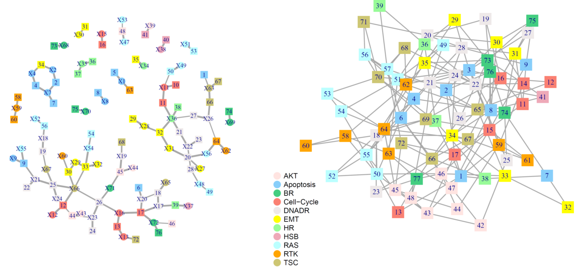
| Gene | Protein | Inclusion | |
|---|---|---|---|
| Probability | |||
| 1 | X63 | 1 | 0.63 |
| 2 | X2 | 2 | 1.00 |
| 3 | X7 | 2 | 0.96 |
| 4 | X4 | 4 | 1.00 |
| 5 | X7 | 4 | 1.00 |
| 6 | X1 | 5 | 1.00 |
| 7 | X20 | 6 | 0.94 |
| 8 | X7 | 7 | 1.00 |
| 9 | X8 | 8 | 1.00 |
| 10 | X9 | 9 | 0.98 |
| 11 | X21 | 9 | 0.77 |
| 12 | X55 | 9 | 0.96 |
| 13 | X11 | 10 | 0.96 |
| 14 | X11 | 11 | 1.00 |
| 15 | X36 | 11 | 0.96 |
| 16 | X12 | 12 | 1.00 |
| 17 | X66 | 12 | 0.98 |
| 18 | X13 | 13 | 1.00 |
| 19 | X16 | 13 | 1.00 |
| 20 | X15 | 16 | 1.00 |
| 21 | X16 | 17 | 1.00 |
| 22 | X17 | 17 | 1.00 |
| 23 | X20 | 17 | 0.95 |
| 24 | X72 | 17 | 0.98 |
| 25 | X17 | 18 | 1.00 |
| 26 | X20 | 18 | 0.58 |
| Gene | Protein | Inclusion | |
|---|---|---|---|
| Probability | |||
| 27 | X65 | 18 | 1.00 |
| 28 | X18 | 19 | 1.00 |
| 29 | X67 | 19 | 0.65 |
| 30 | X27 | 20 | 0.80 |
| 31 | X31 | 20 | 1.00 |
| 32 | X56 | 20 | 0.97 |
| 33 | X22 | 21 | 0.95 |
| 34 | X36 | 21 | 0.97 |
| 35 | X21 | 22 | 1.00 |
| 36 | X22 | 23 | 0.96 |
| 37 | X23 | 24 | 1.00 |
| 38 | X21 | 25 | 0.97 |
| 39 | X24 | 25 | 1.00 |
| 40 | X66 | 25 | 0.92 |
| 41 | X67 | 25 | 0.84 |
| 42 | X16 | 26 | 0.81 |
| 43 | X23 | 26 | 1.00 |
| 44 | X66 | 26 | 0.67 |
| 45 | X71 | 26 | 0.85 |
| 46 | X26 | 27 | 1.00 |
| 47 | X36 | 27 | 0.55 |
| 48 | X22 | 28 | 0.72 |
| 49 | X27 | 28 | 1.00 |
| 50 | X48 | 28 | 0.69 |
| 51 | X28 | 29 | 1.00 |
| 52 | X29 | 30 | 1.00 |
| Gene | Protein | Inclusion | |
|---|---|---|---|
| Probability | |||
| 53 | X60 | 30 | 0.76 |
| 54 | X66 | 30 | 0.82 |
| 55 | X30 | 31 | 1.00 |
| 56 | X28 | 32 | 0.85 |
| 57 | X31 | 32 | 1.00 |
| 58 | X36 | 32 | 0.99 |
| 59 | X29 | 33 | 1.00 |
| 60 | X32 | 33 | 1.00 |
| 61 | X54 | 33 | 1.00 |
| 62 | X66 | 33 | 0.72 |
| 63 | X2 | 34 | 0.92 |
| 64 | X4 | 34 | 0.92 |
| 65 | X34 | 35 | 1.00 |
| 66 | X35 | 36 | 1.00 |
| 67 | X35 | 37 | 1.00 |
| 68 | X36 | 38 | 1.00 |
| 69 | X17 | 39 | 0.91 |
| 70 | X37 | 39 | 1.00 |
| 71 | X38 | 40 | 1.00 |
| 72 | X39 | 41 | 1.00 |
| 73 | X23 | 44 | 0.52 |
| 74 | X24 | 44 | 0.58 |
| 75 | X43 | 44 | 1.00 |
| 76 | X19 | 45 | 1.00 |
| 77 | X44 | 45 | 1.00 |
| 78 | X71 | 45 | 0.82 |
| Gene | Protein | Inclusion | |
|---|---|---|---|
| Probability | |||
| 79 | X72 | 46 | 0.52 |
| 80 | X47 | 48 | 1.00 |
| 81 | X53 | 48 | 0.56 |
| 82 | X48 | 49 | 0.65 |
| 83 | X11 | 50 | 0.59 |
| 84 | X49 | 50 | 1.00 |
| 85 | X51 | 53 | 0.94 |
| 86 | X54 | 54 | 0.80 |
| 87 | X18 | 56 | 0.81 |
| 88 | X52 | 56 | 0.72 |
| 89 | X59 | 58 | 1.00 |
| 90 | X59 | 60 | 1.00 |
| 91 | X1 | 63 | 0.98 |
| 92 | X26 | 64 | 0.52 |
| 93 | X56 | 64 | 1.00 |
| 94 | X62 | 64 | 1.00 |
| 95 | X26 | 66 | 0.91 |
| 96 | X63 | 66 | 1.00 |
| 97 | X63 | 67 | 1.00 |
| 98 | X19 | 68 | 0.80 |
| 99 | X13 | 72 | 0.95 |
| 100 | X68 | 73 | 1.00 |
| 101 | X69 | 74 | 1.00 |
| 102 | X70 | 75 | 0.90 |
| 103 | X72 | 76 | 1.00 |
| Protein | Protein | Inclusion | |
|---|---|---|---|
| Probability | |||
| 1 | 2 | 3 | 1.00 |
| 2 | 3 | 8 | 1.00 |
| 3 | 9 | 11 | 1.00 |
| 4 | 1 | 13 | 1.00 |
| 5 | 1 | 15 | 1.00 |
| 6 | 9 | 15 | 1.00 |
| 7 | 3 | 16 | 1.00 |
| 8 | 11 | 16 | 1.00 |
| 9 | 12 | 16 | 1.00 |
| 10 | 1 | 17 | 1.00 |
| 11 | 2 | 17 | 1.00 |
| 12 | 11 | 17 | 1.00 |
| 13 | 4 | 18 | 1.00 |
| 14 | 16 | 19 | 1.00 |
| 15 | 6 | 20 | 1.00 |
| 16 | 19 | 20 | 1.00 |
| 17 | 6 | 21 | 1.00 |
| 18 | 14 | 22 | 1.00 |
| 19 | 21 | 22 | 1.00 |
| 20 | 18 | 23 | 1.00 |
| 21 | 3 | 24 | 1.00 |
| 22 | 21 | 24 | 1.00 |
| 23 | 22 | 24 | 1.00 |
| 24 | 22 | 25 | 1.00 |
| 25 | 2 | 26 | 1.00 |
| 26 | 8 | 26 | 1.00 |
| 27 | 3 | 27 | 1.00 |
| 28 | 16 | 27 | 1.00 |
| 29 | 2 | 28 | 1.00 |
| 30 | 4 | 28 | 1.00 |
| 31 | 9 | 28 | 1.00 |
| 32 | 20 | 28 | 1.00 |
| 33 | 3 | 29 | 0.54 |
| 34 | 3 | 30 | 1.00 |
| 35 | 8 | 30 | 1.00 |
| 36 | 14 | 30 | 1.00 |
| 37 | 20 | 30 | 1.00 |
| 38 | 11 | 31 | 1.00 |
| 39 | 16 | 31 | 1.00 |
| 40 | 7 | 32 | 1.00 |
| 41 | 32 | 33 | 1.00 |
| 42 | 8 | 34 | 1.00 |
| 43 | 18 | 34 | 1.00 |
| 44 | 24 | 34 | 1.00 |
| 45 | 33 | 34 | 1.00 |
| 46 | 18 | 35 | 1.00 |
| 47 | 24 | 35 | 1.00 |
| Protein | Protein | Inclusion | |
|---|---|---|---|
| Probability | |||
| 48 | 29 | 35 | 1.00 |
| 49 | 22 | 36 | 1.00 |
| 50 | 29 | 36 | 1.00 |
| 51 | 1 | 37 | 1.00 |
| 52 | 36 | 37 | 1.00 |
| 53 | 1 | 38 | 1.00 |
| 54 | 7 | 38 | 1.00 |
| 55 | 37 | 38 | 1.00 |
| 56 | 36 | 39 | 1.00 |
| 57 | 8 | 41 | 1.00 |
| 58 | 14 | 41 | 1.00 |
| 59 | 22 | 41 | 1.00 |
| 60 | 25 | 42 | 1.00 |
| 61 | 17 | 43 | 1.00 |
| 62 | 42 | 43 | 1.00 |
| 63 | 43 | 45 | 1.00 |
| 64 | 44 | 45 | 1.00 |
| 65 | 6 | 46 | 0.76 |
| 66 | 15 | 46 | 1.00 |
| 67 | 33 | 46 | 1.00 |
| 68 | 44 | 46 | 1.00 |
| 69 | 8 | 47 | 1.00 |
| 70 | 42 | 47 | 1.00 |
| 71 | 43 | 47 | 1.00 |
| 72 | 46 | 47 | 1.00 |
| 73 | 43 | 48 | 1.00 |
| 74 | 21 | 49 | 1.00 |
| 75 | 31 | 49 | 1.00 |
| 76 | 6 | 50 | 1.00 |
| 77 | 18 | 50 | 1.00 |
| 78 | 43 | 50 | 1.00 |
| 79 | 46 | 50 | 1.00 |
| 80 | 3 | 51 | 1.00 |
| 81 | 20 | 51 | 1.00 |
| 82 | 49 | 51 | 1.00 |
| 83 | 18 | 52 | 1.00 |
| 84 | 50 | 52 | 1.00 |
| 85 | 51 | 54 | 1.00 |
| 86 | 53 | 54 | 1.00 |
| 87 | 4 | 55 | 1.00 |
| 88 | 6 | 55 | 1.00 |
| 89 | 13 | 55 | 1.00 |
| 90 | 45 | 55 | 1.00 |
| 91 | 52 | 55 | 1.00 |
| 92 | 54 | 55 | 1.00 |
| 93 | 4 | 56 | 1.00 |
| 94 | 2 | 57 | 1.00 |
| Protein | Protein | Inclusion | |
|---|---|---|---|
| Probability | |||
| 95 | 6 | 57 | 1.00 |
| 96 | 39 | 57 | 0.53 |
| 97 | 56 | 57 | 1.00 |
| 98 | 50 | 58 | 1.00 |
| 99 | 1 | 59 | 1.00 |
| 100 | 3 | 59 | 1.00 |
| 101 | 14 | 59 | 1.00 |
| 102 | 44 | 59 | 1.00 |
| 103 | 18 | 60 | 1.00 |
| 104 | 58 | 60 | 1.00 |
| 105 | 15 | 61 | 1.00 |
| 106 | 59 | 61 | 1.00 |
| 107 | 3 | 62 | 1.00 |
| 108 | 49 | 62 | 1.00 |
| 109 | 56 | 62 | 1.00 |
| 110 | 57 | 62 | 1.00 |
| 111 | 58 | 62 | 1.00 |
| 112 | 47 | 63 | 1.00 |
| 113 | 51 | 63 | 1.00 |
| 114 | 58 | 63 | 1.00 |
| 115 | 45 | 64 | 1.00 |
| 116 | 53 | 64 | 1.00 |
| 117 | 54 | 64 | 0.75 |
| 118 | 55 | 64 | 1.00 |
| 119 | 62 | 64 | 1.00 |
| 120 | 63 | 64 | 1.00 |
| 121 | 12 | 65 | 1.00 |
| 122 | 21 | 65 | 1.00 |
| 123 | 33 | 65 | 1.00 |
| 124 | 62 | 65 | 1.00 |
| 125 | 6 | 66 | 1.00 |
| 126 | 23 | 66 | 1.00 |
| 127 | 38 | 66 | 1.00 |
| 128 | 46 | 66 | 1.00 |
| 129 | 65 | 66 | 1.00 |
| 130 | 16 | 67 | 1.00 |
| 131 | 34 | 67 | 0.95 |
| 132 | 61 | 67 | 1.00 |
| 133 | 64 | 67 | 1.00 |
| 134 | 66 | 67 | 1.00 |
| 135 | 22 | 68 | 1.00 |
| 136 | 57 | 68 | 1.00 |
| 137 | 62 | 68 | 1.00 |
| 138 | 2 | 69 | 1.00 |
| 139 | 15 | 69 | 1.00 |
| 140 | 16 | 69 | 1.00 |
| 141 | 18 | 69 | 1.00 |
| Protein | Protein | Inclusion | |
|---|---|---|---|
| Probability | |||
| 142 | 21 | 69 | 1.00 |
| 143 | 48 | 69 | 1.00 |
| 144 | 64 | 69 | 1.00 |
| 145 | 21 | 70 | 0.65 |
| 146 | 37 | 70 | 1.00 |
| 147 | 53 | 70 | 1.00 |
| 148 | 56 | 70 | 1.00 |
| 149 | 57 | 70 | 1.00 |
| 150 | 68 | 70 | 1.00 |
| 151 | 69 | 70 | 1.00 |
| 152 | 20 | 71 | 1.00 |
| 153 | 56 | 71 | 0.79 |
| 154 | 70 | 71 | 1.00 |
| 155 | 17 | 72 | 1.00 |
| 156 | 45 | 72 | 1.00 |
| 157 | 57 | 72 | 1.00 |
| 158 | 66 | 72 | 1.00 |
| 159 | 14 | 73 | 1.00 |
| 160 | 26 | 73 | 0.94 |
| 161 | 29 | 73 | 1.00 |
| 162 | 35 | 73 | 0.90 |
| 163 | 65 | 73 | 1.00 |
| 164 | 4 | 74 | 1.00 |
| 165 | 7 | 74 | 1.00 |
| 166 | 25 | 74 | 1.00 |
| 167 | 31 | 74 | 1.00 |
| 168 | 65 | 74 | 1.00 |
| 169 | 73 | 74 | 1.00 |
| 170 | 9 | 75 | 1.00 |
| 171 | 27 | 75 | 1.00 |
| 172 | 30 | 75 | 1.00 |
| 173 | 31 | 75 | 1.00 |
| 174 | 73 | 75 | 1.00 |
| 175 | 2 | 76 | 1.00 |
| 176 | 8 | 76 | 1.00 |
| 177 | 15 | 76 | 1.00 |
| 178 | 19 | 76 | 1.00 |
| 179 | 24 | 76 | 1.00 |
| 180 | 13 | 77 | 1.00 |
| 181 | 17 | 77 | 1.00 |
| 182 | 23 | 77 | 1.00 |
| 183 | 26 | 77 | 1.00 |
| 184 | 46 | 77 | 1.00 |
| 185 | 48 | 77 | 1.00 |
| 186 | 63 | 77 | 1.00 |
References
- Alquier (2020) Alquier P (2020) Approximate bayesian inference. Entropy (Basel) 22:1272
- Barbieri and Berger (2004) Barbieri MM, Berger JO (2004) Optimal predictive model selection. Annals of Statistics 32(3):870–897
- Basu and Michailidis (2015) Basu S, Michailidis G (2015) Regularized estimation in sparse high-dimensional time series models. The Annals of Statistics 43(4):1535–1567
- Besag (1975) Besag J (1975) Statistical analysis of non-lattice data. Journal of the Royal Statistical Society: Series D (The Statistician) 24(3):179–195
- Bhadra and Mallick (2013) Bhadra A, Mallick BK (2013) Joint high-dimensional Bayesian variable and covariance selection with an application to eQTL analysis. Biometrics 69(2):447–457
- Bissiri et al. (2016) Bissiri P, Holmes C, Walker S (2016) A general framework for updating belief distributions. Journal of the Royal Statistical Society Ser B 78:1103–1130
- Brown et al. (1998) Brown PJ, Vannucci M, Fearn T (1998) Multivariate Bayesian variable selection and prediction. Journal of the Royal Statistical Society Series B 60:627–641
- Cai et al. (2013) Cai TT, Li H, Liu W, Xie J (2013) Covariate-adjusted precision matrix estimation with an application in genetical genomics. Biometrika 100(1):139–156
- Cao et al. (2019) Cao X, Khare K, Ghosh M (2019) Posterior graph selection and estimation consistency for high-dimensional bayesian dag models. Annals of Statistics 47(1):319–348
- Cao et al. (2020) Cao X, Khare K, Ghosh M, et al. (2020) High-dimensional posterior consistency for hierarchical non-local priors in regression. Bayesian Analysis 15(1):241–262
- Consonni et al. (2017) Consonni G, La Rocca L, Peluso S (2017) Objective Bayes covariate-adjusted sparse graphical model selection. Scandinavian Journal of Statistics 44:741–764
- Deshpande et al. (2019) Deshpande SK, Ročková V, George EI (2019) Simultaneous variable and covariance selection with the multivariate spike-and-slab lasso. Journal of Computational and Graphical Statistics 28(4):921–931
- Friedman et al. (2008) Friedman J, Hastie T, Tibshirani R (2008) Sparse inverse covariance estimation with the graphical lasso. Biostatistics 9(3):432–441
- Van de Geer et al. (2014) Van de Geer S, Bühlmann P, Ritov Y, Dezeure R (2014) On asymptotically optimal confidence regions and tests for high-dimensional models. The Annals of Statistics 42(3):1166–1202
- Ghosh et al. (2021) Ghosh S, Khare K, Michailidis G (2021) Strong selection consistency of bayesian vector autoregressive models based on a pseudo-likelihood approach. Annals of Statistics 49:1267–1299
- Gonzalez and Medici (2014) Gonzalez DM, Medici D (2014) Signaling mechanisms of the epithelial-mesenchymal transition. Science signaling 7(344):re8–re8
- Ha et al. (2020a) Ha MJ, Stingo F, Baladandayuthapani V (2020a) Supplemental material for ‘Bayesian Structure Learning in Multi-layered Genomic Networks’. Github
- Ha et al. (2020b) Ha MJ, Stingo FC, Baladandayuthapani V (2020b) Bayesian structure learning in multi-layered genomic networks. Journal of the American Statistical Association (just-accepted):1–33
- Jalali et al. (2020) Jalali P, Khare K, Michailidis G (2020) B-concord – a scalable bayesian high-dimensional precision matrix estimation procedure. 2005.09017
- Khare et al. (2015) Khare K, Oh S, Rajaratnam B (2015) A convex pseudolikelihood framework for high dimensional partial correlation estimation with convergence guarantees. Journal of the Royal Statistical Society B 77:803–825
- Lee et al. (2020) Lee K, Lee K, Lee J (2020) Post-processed posteriors for banded covariances. arXiv preprint arXiv:201112627
- Lee and Liu (2012) Lee W, Liu Y (2012) Simultaneous multiple response regression and inverse covariance matrix estimation via penalized gaussian maximum likelihood. Journal of multivariate analysis 111:241–255
- Li et al. (2021) Li Y, Datta J, Craig BA, Bhadra A (2021) Joint mean–covariance estimation via the horseshoe. Journal of Multivariate Analysis 183:104716
- Lin et al. (2016a) Lin J, Basu S, Banerjee M, Michailidis G (2016a) Penalized maximum likelihood estimation of multi-layered gaussian graphical models. Journal of Machine Learning Research 17:1–51
- Lin et al. (2016b) Lin L, Drton M, Shojaie A (2016b) High-Dimensional Inference of Graphical Models Using Regularized Score Matching. Electronic Journal of Statistics 10(1):394–422
- Ma and Michailidis (2016) Ma J, Michailidis G (2016) Joint structural estimation of multiple graphical models. Journal of Machine Learning Research 17(166):1–48
- McCarter and Kim (2014) McCarter C, Kim S (2014) On sparse gaussian chain graph models. In: Advances in Neural Information Processing Systems, pp 3212–3220
- Meinshausen and Bühlmann (2006) Meinshausen N, Bühlmann P (2006) High-dimensional graphs and variable selection with the lasso. The Annals of Statistics pp 1436–1462
- Narisetty and He (2014) Narisetty N, He X (2014) Bayesian variable selection with shrinking and diffusing priors. Ann Statist 42:789–817
- Peng et al. (2009a) Peng J, Wang P, Zhou N, Zhu J (2009a) Partial correlation estimation by joint sparse regression models. Journal of the American Statistical Association 104:735–746
- Peng et al. (2009b) Peng J, Wang P, Zhou N, Zhu J (2009b) Partial correlation estimation by joint sparse regression models. Journal of the American Statistical Association 104(486)
- Richardson et al. (2010) Richardson S, Bottolo L, Rosenthal JS (2010) Bayesian models for sparse regression analysis of high dimensional data. In Bernardo, J, Bayarri, M, Berger, J, Dawid, A, Heckerman, D, Smith, A F M, and West, M, editors, Bayesian Statistics 9
- Rothman et al. (2010) Rothman AJ, Levina E, Zhu J (2010) Sparse multivariate regression with covariance estimation. Journal of Computational and Graphical Statistics 19(4):947–962
- Sohn and Kim (2012) Sohn KA, Kim S (2012) Joint estimation of structured sparsity and output structure in multiple-output regression via inverse-covariance regularization. In: International Conference on Artificial Intelligence and Statistics, pp 1081–1089
- Vershynin (2018) Vershynin R (2018) High-Dimensional Probability. Cambridge University Press
- Wang (2012) Wang H (2012) Bayesian graphical lasso models and efficient posterior computation. Bayesian Analysis 7(4):867–886
- Yuan and Zhang (2014) Yuan XT, Zhang T (2014) Partial gaussian graphical model estimation. IEEE Transactions on Information Theory 60(3):1673–1687