Dynamics of small particle inertial migration in curved square ducts

Abstract

Microchannels are well-known in microfluidic applications for the control and separation of microdroplets and cells. Often the objects in the flow experience inertial effects, resulting in dynamics that is a departure from the underlying channel flow dynamics. This paper considers small neutrally buoyant spherical particles suspended in flow through a curved duct having a square cross-section. The particle experiences a combination of inertial lift force induced by the disturbance from the primary flow along the duct, and drag from the secondary vortices in the cross-section, which drive migration of the particle within the cross-section. We construct a simplified model that preserves the core topology of the force field yet depends on a single parameter $\kappa$, quantifying the relative strength of the two forces. We show that $\kappa$ is a bifurcation parameter for the dynamical system that describes motion of the particle in the cross section of the duct. At large values of $\kappa$ there exists an attracting limit cycle, in each of the upper and lower halves of the duct. At small $\kappa$ we find that particles migrate to one of four stable foci. Between these extremes, there is an intermediate-range of $\kappa$ for which all particles migrate to a single stable focus. Noting that the positions of the limit cycles and foci vary with the value of $\kappa$, this behavior indicates that, for a suitable particle mixture, duct bend radius might be chosen to segregate particles by size. We evaluate the time and axial distance required to focus particles near the unique stable node, which determines the duct length required for particle segregation.

37C27,70K05, 70K42, 70K70,76D05

1 Introduction

Inertial lift is a phenomenon, first reported by Segre and Silberberg [17], that causes particles and cells suspended in flow through microscale devices to deviate from fluid streamlines. The applications of this effect are revolutionizing diagnostic medical technologies, the separation and identification of circulating tumor cells (CTCs) being one of many examples [19]. Other general uses include flow cytometry, rare cell isolation, cell cycle synchronization, platelet and bacteria separation, plasma extraction, particle classification, and fluid mixing [12]. While the effect of inertial lift on particle migration has been extensively studied for uni-directional flows [1, 9, 11, 13, 16], many of the devices being used in cutting edge microfluidics have a complex design through which there is a full three-dimensional flow. Some of the more recent advances in this field, experimental and otherwise, are described in several review articles [2, 3, 18].

Inertial migration of a neutrally buoyant spherical particle suspended in flow through a straight duct with square cross-section was considered by Hood et. al [11]. Analysis of the fully enclosed flow is challenging, and to render the problem tractable a combination of perturbation theory and numerical computation was applied. Motivated by their approach, Harding et al. [8] extended this work to consider the inertial migration of a neutrally buoyant spherical particle suspended in flow through curved ducts with square, rectangular and trapezoidal cross-sections; it was found that rectangular and trapezoidal cross-sections had a better ability to separate particles depending on their size and these cross-sections became the primary focus of the results presented. In particular, it was demonstrated that the lateral focusing location within curved ducts with a rectangular cross-section could be approximately characterized by a dimensionless parameter $\kappa$ which approximately quantifies the relative strength of the secondary flow drag to the inertial lift force, these being the primary drivers of particle migration. Although the migration of only a single particle was considered it is reasonable to expect good predictions of the behavior of sufficiently dilute suspensions in which particle-particle interaction is minimal. In this paper we focus on curved ducts with a square cross-section which, as seen in [8], exhibit a variety of interesting migration dynamics that warrant further investigation. This is one aim of the present paper.

A second aim is to construct a model of the migration forces on a particle in a curved duct which is simple to evaluate whilst still capturing the topological structure which is essential for accurate prediction of migration dynamics. While simulation data from [8] can be interpolated directly and applied to the integration of particle trajectories, a simpler closed-form model facilitates rapid prototyping. Existing models in the literature often focus on modeling the inertial lift force as a sum of wall-induced, slip-shear and shear-gradient-induced components. Such models are generally one-dimensional in nature owing to the historical development of this decomposition via a study of particle migration in one-dimensional flows between two plane parallel walls. Rasooli and Çetin [15] remark that the application of such models “for the prediction of equilibria for particles in 3D Poiseuille flow in square and rectangular channels is quite questionable”. They instead use Hood et al.’s approximation of the inertial lift force in straight rectangular ducts [11] for their own particle tracking model applied to flow through curved rectangular ducts. The idea of combining the inertial lift force from a straight duct with drag forces induced from curved duct flow as a simple but useful way to describe behavior in curved ducts was also explored by Harding [5].

Our particle tracking model for neutrally buoyant spherical particles suspended in flow through curved square ducts is similar to that of Rasooli and Çetin [15] but differs in a few key ways: a) the axial particle velocity is taken to be in constant equilibrium with the surrounding fluid, b) the forces within a cross-section are decomposed solely into a secondary flow drag and inertial lift force, and c) both the secondary flow drag and inertial lift force are modeled via relatively simple formulae. The assumption in a), which includes neglect of the added mass force, is reasonable because equilibrium in the main direction of flow is reached quickly compared to the time scale of particle migration. Moreover, as the particle migrates in the cross-sectional plane the change in axial velocity is sufficiently smooth and slow for equilibrium to be maintained. The decomposition in b) comes about after the careful analysis and decomposition of the forces on a neutrally buoyant particle in [8] which, for example, reveals that the centripetal and centrifugal forces are approximately equal and opposite for a neutrally buoyant particle. For c) we use a novel approximation of inertial lift which preserves the topological structure of the zero level curves of the inertial lift force to ensure an accurate prediction of equilibria points over a wide range of problem parameters. Put together, these simplifications result in our Zero Level Fit (ZeLF) model, first introduced here, which expedites the calculation of particle trajectories allowing a detailed study of the resulting dynamical system.

Using the ZeLF model we study the dynamics of particle migration in a curved square duct. We show that there are three regimes, a small $\kappa$ regime in which a small number of stable equilibria exist, a large $\kappa$ regime in which a stable attracting orbit exists, and the transition between these two regimes. This intermediate $\kappa$ regime is of particular interest as it has only one focusing point. For this regime, we investigate the axial distance and time scale required for the focusing to occur, and how these depend on initial particle location in the cross-section. While previous studies have only looked at the dynamics within the cross-section, the axial dynamics are extremely important in the context of applications (e.g. cell isolation and separation) in which it is necessary for particles to be focused by the time they reach the end of the duct.

The paper is organized as follows. Section 2 reviews the previous work done on particle flows in curved ducts. Section 3 describes how the ZeLF model for the particle dynamics is constructed. In particular, this section details the construction of the different components and how they are ultimately assembled for estimating particle trajectories to quickly and easily study the dynamics. In addition, the accuracy of the ZeLF model is shown by comparing it with the numerical model of [8]. The ZeLF model is then used in Section 4 to analyse the migration dynamics of a small particle for the three regimes of small, intermediate and large $\kappa$ value. How these compare with the dynamics predicted by the numerical model of [8] is also illustrated. Conclusions are given in Section 5.

2 Background

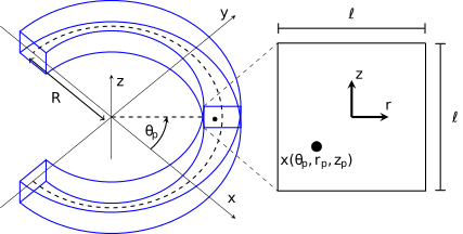
(a)

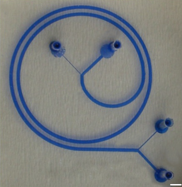
(b)

Figure 1: Configurations of curved ducts. (a) Curved duct with square cross-section containing a spherical particle located at $\mathbf{x}_{p}=\mathbf{x}(\theta_{p},r_{p},z_{p})$. The enlarged view of the cross-section around the particle illustrates the origin of the local $r,z$ coordinates at the center of the duct, as first described in [8]. The bend radius $R$ is with respect to the center-line of the duct and is quite small here for illustration purposes. Note that we do not consider the flow near the inlet/outlet. (b) Photo of an actual curved microchannel, provided by and reproduced with the permission of the Warkiani Laboratory, University of Technology Sydney, Australia. Notice the bend radius is approximately constant for $7/4$ turns. The scale bar on the bottom right is 2cm.

The general setup of our curved square duct is depicted in Figure 1. The horizontal and vertical coordinates within the duct cross-section are $(r,z)\in[-\ell/2,\ell/2]\times[-\ell/2,\ell/2]$ where $\ell$ is the side length of the square cross-section. The cross-sectional coordinates map to points in the three dimensional duct via

(1) $$\mathbf{x}(\theta,r,z)=(R+r)\cos(\theta)\mathbf{i}+(R+r)\sin(\theta)\mathbf{j}+z\mathbf{k}\,,$$

where $\theta$ is angular distance along the duct and $R$ is the bend radius of the duct (measured to the center of the cross-section). The dimensionless parameter $\epsilon:=\ell/(2R)$ is used to characterise the bend radius relative to half the cross-section height.

Let $\bar{p},\bar{\mathbf{u}}$ describe the pressure and velocity fields, respectively, of a steady pressure driven flow through the curved square duct in the absence of any particles. The fluid is assumed to be incompressible with uniform density $\rho$ and uniform viscosity $\mu$. For convenience we separate $\bar{\mathbf{u}}$ into its axial component $\bar{\mathbf{u}}_{a}$ and secondary component $\bar{\mathbf{u}}_{s}$, specifically

$$\bar{\mathbf{u}}_{a} :=(\bar{\mathbf{u}}\cdot\mathbf{e}_{\theta})\mathbf{e}_{\theta}\,,$$

$$\bar{\mathbf{u}}_{s} :=\bar{\mathbf{u}}-\bar{\mathbf{u}}_{a}\,.$$

The maximum of $\bar{\mathbf{u}}_{a}$ is taken to be the characteristic flow velocity and is denoted by $U_{m}$. It is assumed that the Dean number $K=\mathrm{Re}_{c}^{2}\epsilon$, where $\epsilon:=\ell/(2R)$ (as defined earlier) and $\mathrm{Re}_{c}=(\rho/\mu)U_{m}\ell/2$ is the channel Reynolds number, is small enough that the inertia of the fluid flow through the curved duct does not perturb the axial velocity component significantly from the Poiseuille flow obtained in a straight duct. The secondary flow $\bar{\mathbf{u}}_{s}$, consisting of two counter rotating vortices in the cross-sectional plane, scales with $U_{m}\sqrt{K\epsilon}$ [6].

A spherical particle with radius $a<\ell/2$ is then suspended in the fluid flow resulting in the new pressure and velocity fields $p,\mathbf{u}$, respectively. The location of the particle is described by the location of its center $\mathbf{x}_{p}=\mathbf{x}(\theta_{p},r_{p},z_{p})$. We assume the particle is free to spin, which features in the calculation of the forces that influence its motion [8]. However, in this study we do not track the particle spin as our aim is to produce a simplified model of the particle’s position. The flow fields $p,\mathbf{u}$ are non-steady due to the motion of the spherical particle suspended in it. However, as in [8], we move to the reference frame rotating with the cross-section containing the particle center, in which the angular coordinate is $\theta^{\prime}=\theta-\theta_{p}$ and the radial and vertical coordinates remain unchanged. In this rotating reference frame, the fluid motion may be taken as steady and a disturbance flow $q^{\prime},\mathbf{v}^{\prime}$ is introduced which describes the difference between $\bar{p},\bar{\mathbf{u}}$ and $p,\mathbf{u}$ in that frame. The force on the particle can be decomposed into three components: a gravity/buoyancy balance $\mathbf{F}_{g}$, a centrifugal/centripetal force balance $\mathbf{F}_{c}$ and a remaining hydrodynamic component $\mathbf{F}_{nb}$. There is an analogous decomposition of the torque which we do not describe in detail.

A recent paper explored the effects of non-neutral particle buoyancy for curved ducts having a rectangular cross-section [7]. Perturbations due to non-neutral buoyancy were found to be small for Froude numbers larger than $3$, $\mathrm{Fr}^{2}=U_{m}^{2}a/(g\ell^{2})$, and particle density $\rho_{p}$ satisfying $|\rho_{p}-\rho|\leq\rho/2$. Since this is the case for typical applications of inertial microfluidics, for simplicity, we here restrict attention to neutrally buoyant particles.

For a neutrally buoyant particle (for which $\mathbf{F}_{g}=0$ and $\mathbf{F}_{c}\approx 0$ once axial equilibrium is achieved) only the hydrodynamic force component remains, namely

$$\mathbf{F}_{nb}=\int_{|\mathbf{x}^{\prime}-\mathbf{x}_{p}^{\prime}|=a}\mathbf{n}\cdot\left(-q^{\prime}\mathbf{I}+\mu\left(\nabla^{\prime}v^{\prime}+\nabla^{\prime}v^{\prime\,T}\right)\right)\,dS^{\prime}\,,$$

where $|\mathbf{x}^{\prime}-\mathbf{x}_{p}^{\prime}|=a$ is the surface of the particle, primes denote variables in the rotating reference frame, and $\mathbf{n}$ is the outward pointing normal. Upon non-dimensionalizing for a viscous flow, using the characteristic length $a$ and velocity $U=U_{m}a/\ell$, one may perform a perturbation expansion of $q^{\prime},\mathbf{v}^{\prime}$ with respect to the particle Reynolds number $\mathrm{Re}_{p}=(\rho/\mu)U_{m}a^{2}/\ell$, which is assumed to be sufficiently small. Notice that particles are expected to quickly approach terminal velocity as determined by Stokes’ drag law and, thereafter, $\mathrm{Re}_{p}$ is the effective Stokes number during particle migration. For convenience and since $\bar{\mathbf{u}}_{s}$ scales with $U_{m}\sqrt{K\epsilon}=\mathrm{Re}_{p}U\kappa$, where

(2) $$\kappa=\ell^{4}/(4a^{3}R),$$

the secondary component of the background flow velocity is considered to be $\mathcal{O}(\mathrm{Re}_{p})$. Consequently, the leading order component of $\mathbf{F}_{nb}$ describes the primary force balance governing the axial velocity of the particle $u_{p}=d\theta_{p}/dt$ (and analogously the leading order component of the torque describes the primary balance governing its spin $\mathbf{\Omega}_{p}$).

The first order component of $\mathbf{F}_{nb}$ describes the forces governing particle migration within the cross-section, specifically the inertial lift $\mathbf{L}$ and secondary flow drag $\mathbf{D}$. The perturbation analysis yields [11]

(3) $$\mathbf{L}\propto\rho U_{m}^{2}a^{4}/\ell^{2}=\mu aU\mathrm{Re}_{p}$$

and, recalling that $\bar{\mathbf{u}}_{s}\propto\mathrm{Re}_{p}U\kappa$ and using the Stokes drag law to approximate the secondary drag force, it follows that

(4) $$\mathbf{D}\approx 6\pi\mu a\bar{\mathbf{u}}_{s}\propto\mu aU\mathrm{Re}_{p}\kappa\,.$$

Therefore, one expects $\mathbf{D}\propto\kappa\mathbf{L}$.

Computational approximations of $\mathbf{L}$ and $\mathbf{D}$ have been previously obtained over several cross-sectional shapes (square, rectangular and trapezoidal), in each case for a number of particle sizes and duct bend radii, including for straight ducts ($R\rightarrow\infty$) [8]. A key factor in determining the stability of equilibria and the existence of slow manifolds is the intersection of zero level curves of the $r$ and $z$ components of the net migration force $\mathbf{L}+\mathbf{D}$. Using these, a number of significantly different types of migration dynamics were identified. For rectangular cross-sectional shape in particular, but also for trapezoidal cross-sections, these were found to depend on the value of $\kappa$.

Ducts with square cross-sections were less studied in [8] but three different types of migration dynamics were identified, characterized by four stable equilibria, a single stable equilibrium, and a pair of stable limit cycles. In this paper, we undertake a detailed examination of migration dynamics in ducts with square cross-sectional shapes. For this purpose, it is desirable to construct a simpler model, which we call the Zero Level Fit (ZeLF) model, which is more tractable for studying the dynamical system of the particle motion in depth.

3 Constructing the ZeLF model

The inertial lift $\mathbf{L}$ experienced by the particle is primarily due to the disturbance of the axial flow along the duct. We assume that $\mathbf{L}$ is well approximated by that for the case of flow through a duct with the same cross-section in the limit $R\rightarrow\infty$ ($\epsilon\rightarrow 0$). To this, we add the effect of drag force $\mathbf{D}$ approximated by the Stokes drag law applied to the secondary velocity field $\bar{\mathbf{u}}_{s}$ describing the flow vortices in the cross-section that are due to the curvature of the duct also obtained for the limit $\epsilon\rightarrow 0$. Specifically, we compute $\hat{\mathbf{u}}_{s}=\lim_{R\to\infty}\frac{\bar{\mathbf{u}}_{s}}{U_{m}\sqrt{K\epsilon}}$ and then subsequently approximate $\bar{\mathbf{u}}_{s}$ as $\bar{\mathbf{u}}_{s}\approx U_{m}\sqrt{K\epsilon}\hat{\mathbf{u}}_{s}$. A similar model was briefly explored in [5], focusing on a duct having a rectangular cross-section and using numerical simulation data to compute the forces; for a sufficiently small ratio of duct height $\ell$ to bend radius $R$, the predicted net force driving particle migration was found to be similar to that of the more complex model [8] summarized in the previous section.

However, in contrast to the model of [5], here we fit simple model functions to simulation data for a small particle suspended in flow through a curved duct having a square cross-section and use these functions to estimate the force components. Our model functions preserve the topology of the zero level sets for the inertial lift and drag allowing us to retain the correct migration dynamics for ducts with large bend radius. Additionally, the model smooths over some of the numerical noise/error which is present in the simulation data.

A weakness of this modeling approach is that it may not be appropriate for ducts having a smaller bend radius where the curved geometry of the duct has a noticeable influence on both the inertial lift force and the secondary drag force. As the bend radius increases, the influence of the curved geometry on both of these components decays. Therefore our modeling of both the inertial lift force and secondary drag forces are expected to be most accurate for ducts having a large bend radius compared with the cross-sectional width.

Understanding the axial distance traveled by a particle during migration is crucial to the design of devices for particle focusing and separation. Hence, herein we couple this to the cross-sectional dynamics in a simplified manner. We take the axial velocity of the particle to always be equal to the terminal velocity if it were to remain fixed at its current cross-section location. This is a reasonable assumption because the axial velocity is expected to reach equilibrium on a much faster time scale than that of the cross-sectional migration. Further, since the axial velocity of the particle (at equilibrium) is similar to that of the background flow (there is a small ‘slip’ but it is order $(a/\ell)^{2}$) then this may be approximated by $\bar{\mathbf{u}}_{a}$$(r_{p},z_{p})$. Similar to $\bar{\mathbf{u}}_{s}$, we approximate $\bar{\mathbf{u}}_{a}$ with a simple model function for the limit $\epsilon\rightarrow 0$.

In the remainder of the paper we describe our model non-dimensionalising the cross-sectional coordinates according to

(5) $$(r,z)=\left(\frac{\ell}{2}\tilde{r},\frac{\ell}{2}\tilde{z}\right)\,.$$

This is most convenient because the rescaled cross-sectional domain $(\tilde{r},\tilde{z})\in[-1,1]\times[-1,1]$ is independent of any physical parameters (in contrast to scaling with respect to the particle radius $a$ for which the non-dimensionalized duct dimensions are $\ell/a$).

The following subsections outline the construction of the different model components before describing how they are assembled for the computation of particle trajectories.

3.1 Modeling the inertial lift force

We first give the model for the inertial lift acting on a particle and then discuss its derivation. The dimensionless component of lift in the $r$ direction within the cross-section, for a particle with position $(\tilde{r}_{p},\tilde{z}_{p})=(\tilde{r},\tilde{z})$, is approximated by

(6) $$\hat{L}_{r}(\tilde{r},\tilde{z})=\tilde{r}\left(1-12.7\tilde{r}^{6}-24.8\tilde{z}^{6}\right)\exp\left(2.95-1.43\tilde{r}^{2}-4.23\tilde{z}^{2}-1.98\tilde{r}^{4}\right.\\ \left.+5.28\tilde{r}^{2}\tilde{z}^{2}-1.10\tilde{z}^{4}+2.35\tilde{r}^{6}-1.16\tilde{r}^{4}\tilde{z}^{2}-7.16\tilde{r}^{2}\tilde{z}^{4}+3.51\tilde{z}^{6}\right).$$

Similarly, because of the expected symmetry for a straight duct with square cross-section, the component in the $z$ direction is approximated as

$$\hat{L}_{z}(\tilde{r},\tilde{z})=\hat{L}_{r}(\tilde{z},\tilde{r}).$$

In the dimensional setting these two inertial lift force components are

$$L_{r},L_{z}=\rho U_{m}^{2}\frac{a^{4}}{\ell^{2}}\hat{L}_{r},\rho U_{m}^{2}\frac{a^{4}}{\ell^{2}}\hat{L}_{z}\,.$$

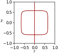
(a) The zero level set curve of $L_{r}$

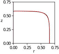
(b) Zoom of the zero level set curve of $L_{r}$

Figure 2: Fit of the zero level set curve of $f(\tilde{r},\tilde{z})=\tilde{r}(1-12.7\tilde{r}^{6}-24.8\tilde{z}^{6})$ (in red) with that of $\tilde{L}_{r}$ from finite element computations from [8] (in black). Figure (a) shows the two over the entire cross-section whereas figure (b) zooms into a portion of the upper right quadrant. The difference between the two is difficult to discern at both scales.

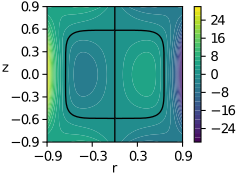
(a) Inertial lift model $\hat{L}_{r}$

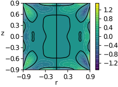
(b) Error of $\hat{L}_{r}$

Figure 3: Model of the inertial lift force $\hat{L}_{r}(\tilde{r},\tilde{z})$: (a) $\hat{L}_{r}$ over the cross-section excluding a small region around the walls; (b) the difference between the model and results computed from finite element solutions [8].

The inertial lift force model was constructed as follows. First the factor preceding the exponential in $\hat{L}_{r}$, $f(\tilde{r},\tilde{z})=\tilde{r}(1-12.7\tilde{r}^{6}-24.8\tilde{z}^{6})$, was determined by trial and error to give a good match between its zero level contour and the zero level contour of an interpolation of $L_{r}$ data computed via numerical simulations for a small particle (specifically with $a/\ell=1/20$) in a straight duct as described in [8]; see Figure 2. This ensures the prediction of the correct location and stability of equilibria for a straight duct. The exponential factor, with exponent consisting of a polynomial in $\tilde{r},\tilde{z}$, was then added to improve the global accuracy of the model in a way that does not modify the zero level contours. The coefficients of the polynomial (in the exponent) were obtained via a constrained least squares fitting to the interpolation of the $L_{r}$ data from the numerical simulations. There is a classical trade-off between accuracy and simplicity of the model in determining a suitable degree of the polynomial within the exponent. Compared with the simulation data, the specific model (6) achieves a $L_{2}$ relative error of $3.8\%$, see Figure 3.

3.2 Modeling the secondary drag force

The secondary drag force on the particle is approximated by combining Stokes’ drag law with the velocity of the secondary component of the fluid flow through a curved duct in the limit $\epsilon\rightarrow 0$. The secondary component consists of two counter-rotating vortices which are orthogonal to the main direction of flow. For a slow laminar flow through a curved duct, it can be shown that the velocity of the secondary component scales as $U_{m}\sqrt{K\epsilon}=\epsilon\mathrm{Re}_{c}U_{m}$ [6, 8]. The two velocity components can be described via a stream-function $\Phi(\tilde{r},\tilde{z})$, specifically with $-\partial\Phi/\partial\tilde{z}$ and $\partial\Phi/\partial\tilde{r}$ describing the velocity in the $\tilde{r}$ and $\tilde{z}$ directions, respectively.

The fundamental scale and topology of $\Phi$ is approximated as

$$\Phi_{0}(\tilde{r},\tilde{z})=-0.01591\epsilon\mathrm{Re}_{c}U_{m}(1-\tilde{r}^{2})^{2}\tilde{z}(1-\tilde{z}^{2})^{2}\,.$$

This approximation ensures that both $-\partial\Phi/\partial\tilde{z}$ and $\partial\Phi/\partial\tilde{r}$ are zero on the duct walls, describes two counter rotating vortices with the correct orientation, has the desired odd symmetry with respect to $\tilde{z}$, and has even symmetry with respect to $\tilde{r}$ as required in the limit $\epsilon\rightarrow 0$. The factor $0.01591$ was determined to fit the velocity fields obtained from a finite difference solution of the Navier–Stokes equations governing the background flow in the limit $\epsilon\rightarrow 0$ and at small flow rate.

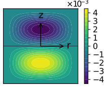
(a) Stream-function model $\Phi_{1}$

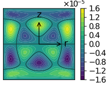
(b) Error of $\Phi_{1}$

Figure 4: Model of the secondary vortices: (a) streamfunction $\Phi_{1}(r,z)$ and (b) the difference between $\Phi_{1}(r,z)$ and the streamfunction from a finite difference computation over the cross-section in the limit $\epsilon\rightarrow 0$.

The accuracy of the secondary velocity approximation can be improved with the addition of further terms. We have performed an $L_{2}$ fit of the model

$$\Phi_{N}(\tilde{r},\tilde{z})=\Phi_{0}(\tilde{r},\tilde{z})\sum_{n=0}^{N}\sum_{i=0}^{n}\beta_{2i,2(n-i)}\tilde{r}^{2i}\tilde{z}^{2(n-i)},$$

for $N\in\mathbb{N}$, to the stream-function computed from the above mentioned finite difference solution of the Navier–Stokes equations. Fits were determined for several $N$ but $N=1$ was found to be sufficiently accurate for our study. In particular, we obtained

$$\Phi_{1}(\tilde{r},\tilde{z}) =\Phi_{0}(\tilde{r},\tilde{z})(0.9833+0.2289\tilde{r}^{2}-0.0178\tilde{z}^{2})$$

where the coefficients have been rounded to four decimal places. A plot of the approximation $\Phi_{1}$ is shown in Figure 4 alongside a plot of the error with respect to the finite-difference solution. The relative error of $\Phi_{1}$ is found to be $0.3\%$ making it sufficiently accurate for the study of dynamics herein.

For a small spherical particle, the drag force within the cross-sectional plane can be estimated using Stokes’ drag law in conjunction with the velocities obtained from the stream-function $\Phi_{1}$. Specifically, for a small particle suspended in the flow and which is not moving with respect to the $\tilde{r},\tilde{z}$ coordinates, one can use the approximation

$$D_{r},D_{z}=-6\pi\mu a\frac{\partial\Phi_{1}}{\partial\tilde{z}},6\pi\mu a\frac{\partial\Phi_{1}}{\partial\tilde{r}}$$

for the radial and vertical components of the drag force respectively. Taking the scaling of $\Phi_{1}$ into account, it is reasonable to non-dimensionalize the secondary drag force according to

$$D_{r},\,D_{z} =\mu a\epsilon\real_{c}U_{m}\tilde{D}_{r},\,\mu a\epsilon\real_{c}U_{m}\tilde{D}_{z}$$

$$=\rho U_{m}^{2}\frac{a\ell^{2}}{4R}\tilde{D}_{r},\,\rho U_{m}^{2}\frac{a\ell^{2}}{4R}\tilde{D}_{z}\,.$$

It is important to note that this approximation will not be accurate when the particle is very close to a wall, or for larger particles. The true drag coefficient is larger for increasing particle size, and additionally the drag coefficient increases when the particle approaches a wall. Since our interest is primarily smaller particles and their dynamics away from the walls we stick with Stokes’ drag law to maintain the simplicity of the model.

3.3 Modeling the axial velocity

The particle travels with an axial velocity which is close to that of the background fluid flow. For a slow laminar fluid flow through a curved square duct (with no particles), the axial velocity field is quite close to Poiseuille flow in a straight square duct, specifically within $O(\epsilon)$. With $U_{m}$ denoting the maximum axial velocity, then a simple approximation of the dimensionless Poiseuille flow is given by

(7) $$u_{0}(\tilde{r},\tilde{z})=U_{m}(1-\tilde{r}^{2})(1-\tilde{z}^{2})\,.$$

This approximation attains the expected maximum, satisfies no-slip boundary conditions on the walls, and has the even symmetry with respect to $r$ and $z$ that is expected for this flow.

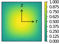
(a) Axial velocity model $u_{1}$

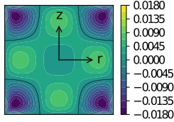
(b) Error of $u_{1}$

Figure 5: (a) Model function for the axial velocity $u_{1}(\tilde{r},\tilde{z})/U_{m}$ and (b) the difference between this and a finite difference computation of Poiseuille flow through a straight square duct with unit wall length.

The accuracy of the simple approximation (7) degrades away from the wall and the center, and can be improved by the addition of further terms in a similar manner to that used above for the streamfunction. Thus, we perform a simple $L_{2}$ fit of the model

(8) $$u_{N}(\tilde{r},\tilde{z})=u_{0}(\tilde{r},\tilde{z})\left(1+\sum_{n=1}^{N}\sum_{i=0}^{n}\alpha_{2i,2(n-i)}\tilde{r}^{2i}\tilde{z}^{2(n-i)}\right),$$

for a given $N\in\mathbb{N}$, with an axial velocity field computed from a finite difference solution of Poiseuille flow in a straight duct. The general form (8) retains all of the features of $u_{0}$ described above but provides a better approximation for increasing $N$. We constructed approximations for several $N$ but here too found that $N=1$ was sufficiently accurate for our study. Specifically, we obtained

$$u_{1}(\tilde{r},\tilde{z})=u_{0}(\tilde{r},\tilde{z})\left(1+0.1818(\tilde{r}^{2}+\tilde{z}^{2})\right),$$

where the coefficient has been rounded to four decimal places. A plot of the approximation $u_{1}$ is shown in Figure 5 alongside a plot of the error $u_{1}-u_{a}$ (both scaled with $U_{m}$) where $u_{a}=\lim_{R\rightarrow\infty}\bar{\mathbf{u}}_{a}\cdot\mathbf{e}_{\theta}$, i.e. the axial flow through a straight square duct. The relative error $\|u_{1}-u_{a}\|_{2}/\|u_{a}\|_{2}$ is found to be $1.1\%$ making $u_{1}$ sufficiently accurate for the study of dynamics herein. The terminal velocity of a particle is thus approximated as

$$u_{p}\approx u_{1}(r_{p},z_{p})\,.$$

3.4 Putting the model together

We now approximate the net force on the particle in the $r,z$ directions as

$$F_{r}=L_{r}+D_{r}\,,\quad F_{z}=L_{z}+D_{z}\,,$$

respectively. If we non-dimensionalize $F_{r},F_{z}$ with the same scale as $L_{r},L_{z}$, that is

$$F_{r}=\rho U_{m}^{2}a^{4}/\ell^{2}\hat{F}_{r}\,,\quad F_{z}=\rho U_{m}^{2}a^{4}/\ell^{2}\hat{F}_{z}\,,$$

then we obtain

$$\hat{F}_{r}=\hat{L}_{r}+\kappa\tilde{D}_{r}\,,\quad\hat{F}_{z}=\hat{L}_{z}+\kappa\tilde{D}_{z}\,,$$

with $\kappa=\ell^{4}/(4a^{3}R)$ as defined in (2). This highlights the fact that $\kappa$ describes the magnitude of the secondary drag force relative to the inertial lift force.

Using Stokes’ drag law, the terminal velocity of a small particle due to the net migration force is

$$v_{r}=\frac{F_{r}}{6\pi\mu a}=\frac{L_{r}+D_{r}}{6\pi\mu a}\,,\quad v_{z}=\frac{F_{z}}{6\pi\mu a}=\frac{L_{z}+D_{z}}{6\pi\mu a}\,.$$

In this study, it will be convenient to non-dimensionalize these velocities according to the secondary fluid velocity scale (rather than a scaling based on the inertial lift force). This is because we generally expect the secondary flow to be the dominant effect for a small particle and the inertial lift force can be viewed as a perturbation to this. In particular, we introduce

$$v_{r}=\epsilon\mathrm{Re}_{c}U_{m}\tilde{v}_{r}\,,\quad v_{z}=\epsilon\mathrm{Re}_{c}U_{m}\tilde{v}_{z}\,.$$

Consequently, we express $\tilde{v}_{r},\tilde{v}_{z}$ as

$$\tilde{v}_{r}=\frac{1}{6\pi}\left(\frac{\hat{L}_{r}}{\kappa}+\tilde{D}_{r}\right)\,,\quad\tilde{v}_{z}=\frac{1}{6\pi}\left(\frac{\hat{L}_{z}}{\kappa}+\tilde{D}_{z}\right)\,.$$

Then, the trajectory of a particle with center $(\tilde{r}_{p},\tilde{z}_{p})$ is modeled via the first order system of ordinary differential equations

(9a) $$\frac{d\tilde{r}_{p}}{d\tilde{t}} =\tilde{v}_{r}\left(\tilde{r}_{p},\tilde{z}_{p}\right)\,,$$

(9b) $$\frac{d\tilde{z}_{p}}{d\tilde{t}} =\tilde{v}_{z}\left(\tilde{r}_{p},\tilde{z}_{p}\right)\,,$$

where $\tilde{t}$ is dimensionless time, related to physical time $t$ by $t=R\tilde{t}/(U_{m}\mathrm{Re}_{c})$.

Observe that our model of particle migration depends only on the cross-sectional coordinate $(\tilde{r}_{p},\tilde{z}_{p})$ and is independent of the current angular location within the curved duct $\theta_{p}$. In order to study how far a particle travels through the curved duct over the time scale at which inertial migration takes place it is necessary to re-incorporate the axial motion into the model. In practice, particles lag slightly from the surrounding fluid velocity. However, for a small particle, this lag is sufficiently small that it is reasonable to take the background fluid velocity at the particle center as an approximation of the particle’s axial velocity. Therefore, we can incorporate this into our system of ordinary differential equations (9) by adding

(10) $$\frac{d\tilde{s}_{p}}{d\tilde{t}}=\frac{d}{d\tilde{t}}(\mathrm{Re}_{c}\theta_{p})=\frac{1}{(1+\epsilon\tilde{r}_{p})}\frac{u_{1}\left(\tilde{r}_{p},\tilde{z}_{p}\right)}{U_{m}}\,,$$

where $\theta_{p}$ tracks the angular coordinate of the particle in the curved duct and $\tilde{s}_{p}=\mathrm{Re}_{c}\theta_{p}$ is the corresponding dimensionless arc-length along the central axis of the channel that is related to the physical arc length ${s}_{p}=R\theta_{p}$ by

(11) $$\tilde{s}_{p}=\frac{\mathrm{Re}_{c}}{R}s_{p}\,.$$

We refer to $\tilde{s}_{p}$ as the distance the particle has travelled down the channel, where $\theta_{p}(0)=\tilde{s}_{p}(0)=0$. Finally, in keeping with the assumption made in developing this model, we take the $\epsilon\rightarrow 0$ limit of (10).

To summarise, the complete ZeLF model is described by the first-order system of ordinary differential equations, involving just the single dimensionless parameter $\kappa$,

(12a) $$\frac{d\tilde{r}_{p}}{d\tilde{t}} =\frac{1}{6\pi\kappa}\tilde{r}_{p}\left(1-12.7\tilde{r}_{p}^{6}-24.8\tilde{z}_{p}^{6}\right)\exp\left(2.95-1.43\tilde{r}_{p}^{2}-4.23\tilde{z}_{p}^{2}-1.98\tilde{r}_{p}^{4}\right.\,$$

$$\hskip 56.9055pt\left.+5.28\tilde{r}_{p}^{2}\tilde{z}_{p}^{2}-1.10\tilde{z}_{p}^{4}+2.35\tilde{r}_{p}^{6}-1.16\tilde{r}_{p}^{4}\tilde{z}_{p}^{2}-7.16\tilde{r}_{p}^{2}\tilde{z}_{p}^{4}+3.51\tilde{z}_{p}^{6}\right)$$

$$\quad+0.01591(1-\tilde{r}_{p}^{2})^{2}(1-\tilde{z}_{p}^{2})\big{(}0.9833+0.2289\tilde{r}_{p}^{2}$$

$$\hskip 142.26378pt-4.9699\tilde{z}_{p}^{2}-1.1445\tilde{r}_{p}^{2}\tilde{z}_{p}^{2}+0.1246\tilde{z}_{p}^{4}\big{)}\,,$$

(12b) $$\frac{d\tilde{z}_{p}}{d\tilde{t}} =\frac{1}{6\pi\kappa}\tilde{z}_{p}\left(1-24.8\tilde{r}_{p}^{6}-12.7\tilde{z}_{p}^{6}\right)\exp\left(2.95-4.23\tilde{r}_{p}^{2}-1.43\tilde{z}_{p}^{2}-1.10\tilde{r}_{p}^{4}\right.$$

$$\hskip 56.9055pt\left.+5.28\tilde{r}_{p}^{2}\tilde{z}_{p}^{2}-1.98\tilde{z}_{p}^{4}+3.51\tilde{r}_{p}^{6}-7.16\tilde{r}_{p}^{4}\tilde{z}_{p}^{2}-1.16\tilde{r}_{p}^{2}\tilde{z}_{p}^{4}+2.35\tilde{z}_{p}^{6}\right)$$

$$\quad+0.01591\tilde{r}_{p}(1-\tilde{r}_{p}^{2})\tilde{z}_{p}(1-\tilde{z}_{p}^{2})^{2}\big{(}3.4754+1.3734\tilde{r}_{p}^{2}-0.0712\tilde{z}_{p}^{2}\big{)}\,,$$

(12c) $$\frac{d\tilde{s}_{p}}{d\tilde{t}} =\left(1+0.1818(\tilde{r}_{p}^{2}+\tilde{z}_{p}^{2})\right)(1-\tilde{r}_{p}^{2})(1-\tilde{z}_{p}^{2})\,.$$

Results from this model are straightforward to translate from dimensionless to dimensional coordinates as needed.

4 Results of the ZeLF model

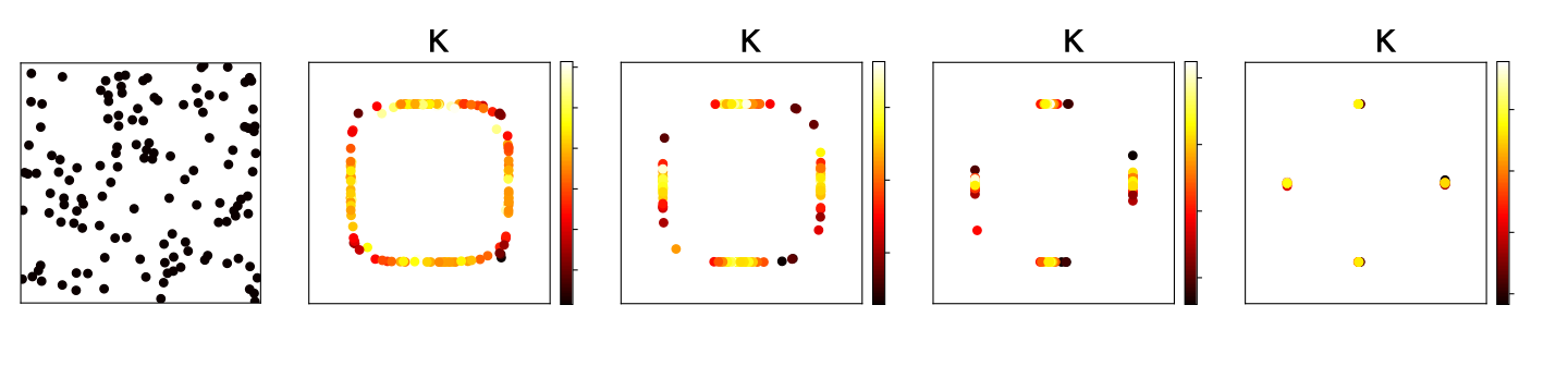
(a) $\kappa=1$

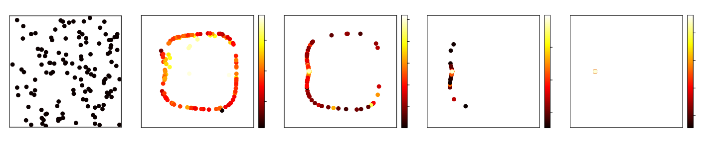
(b) $\kappa=25$

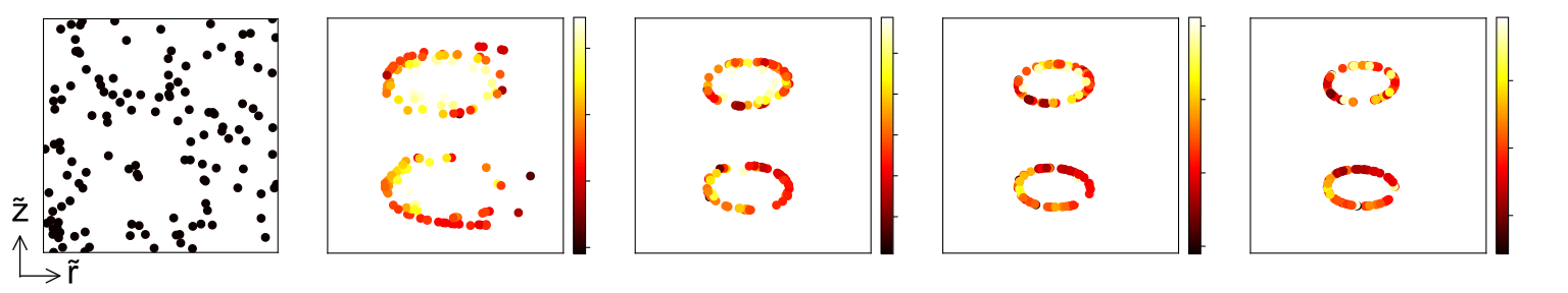
(c) $\kappa=200$

Figure 6: Cross-sectional positions of 128 particles, initially randomly distributed within the cross-section, $[-1,1]\crossproduct[-1,1]$. Each snapshot of the cross-section corresponds from left to right to the time $\tilde{t}=0,2\kappa,8\kappa,15\kappa,$ and $30\kappa$, and from top to bottom (a) small, (b) intermediate, and (c) large $\kappa$. The color scheme shows the axial distance each particle has traveled, calculated by (12c).

In this section, we investigate particle motion and its dependence on $\kappa$ using the ZeLF model. Figure 6 illustrates the migration of particles via five snapshots in time for three distinct $\kappa$ values. The particles migrate towards a single fixed point ($\kappa=25$), one of multiple fixed points ($\kappa=1$) or to a stable orbit ($\kappa=200$). The particle color indicates the dimensionless distance $\tilde{s}_{p}$ traveled down the channel by the particle.

We observe three distinct behaviors, here termed “multi-focus”, “unique-focus” and “periodic orbit”, corresponding to $\kappa$ small ($\kappa\lesssim 10$), intermediate ($10\lesssim\kappa\lesssim 25$), and large ($\kappa\gtrsim 25$). Since we are interested in the long term behavior of the particles we only discuss the long-time limit sets ($\omega$-limit sets [4]). The limit sets are composed of equilibria, which are classified as stable nodes or foci, saddle points, and unstable nodes by their eigenvalues, and limit cycles, also classified as either stable or unstable by their Poincaré map.

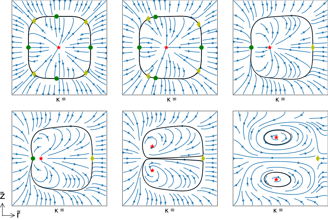
Figure 7: Particle trajectories for different $\kappa$ values within the cross-section, $[-1,1]\crossproduct[-1,1]$. The equilibria are in different colors and shapes: stable nodes (green $\bullet$), saddle points (yellow $\diamondsuit$) and unstable nodes (red $\star$). For $\kappa\leq 25$, the black line represents the heteroclinic orbit that connects the saddle to the stable equilibria. For $\kappa\geq 30$, the black line represents the limit cycle.

4.1 Multi-focus behavior (small $\kappa$)

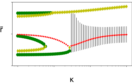
(a) $\kappa$-$\tilde{r}$ position

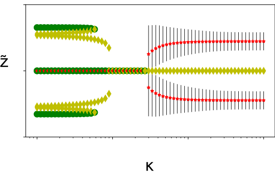
(b) $\kappa$-$\tilde{z}$ position

Figure 8: Equilibrium positions and the limit cycle range as a function of $\kappa$. The equilibria are in different colors and shapes: stable nodes (green $\bullet$), saddle points (yellow $\diamondsuit$) and unstable nodes (red $\star$). The range of the limit cycles are shown in black vertical lines.

For small $\kappa$, there are multiple stable nodes or focusing points near the center of each side of the cross-section, multiple saddle points near the corners of the cross-section, and one unstable node in the middle (Figure 7ab). For each saddle point, there is a heteroclinic orbit that connects to a stable node which acts as a slow manifold. The particles quickly migrate onto one of these heteroclinic orbits, and then slowly converge to the stable node (Figure 6(a)). Therefore, the migration velocity of the particle on the slow manifold determines the time needed for the particles to converge to the stable nodes. These particle trajectories are similar to those in a straight duct which is expected since as $R\rightarrow\infty$, $\kappa\rightarrow 0$ [8, 10].

4.2 Unique focus behavior (intermediate $\kappa$)

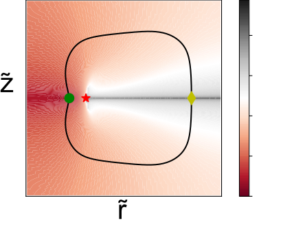
(a)

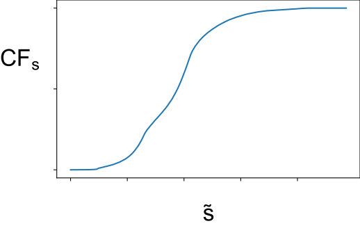
(b)

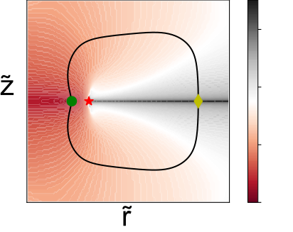
(c)

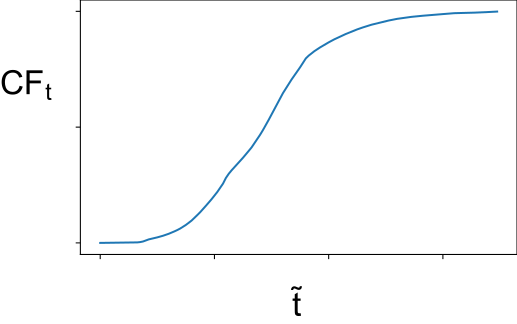
(d)

Figure 9: On the left are heat maps of the cross-section, $[-1,1]\crossproduct[-1,1]$, that show the (a) axial distance $\tilde{s}_{p}^{*}$ and (c) time $\tilde{t}^{*}$, defined in (13), required to focus from a position in the cross-section to the stable equilibrium point for $\kappa=25$. The equilibria are shown in different colors and shapes: stable nodes (green $\bullet$), saddle points (yellow $\diamondsuit$) and unstable nodes (red $\star$). The black solid line represents the heteroclinic orbit connecting the saddle to the stable node. On the right, the graphs show (b) $CF_{s}$ versus $\tilde{s}$ and (d) $CF_{t}$ versus $\tilde{t}$ as defined in (14), i.e. the fraction of the cross-sectional area from which particles have focused within the given distance $\tilde{s}$ and time $\tilde{t}$.

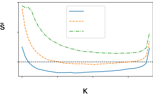
(a)

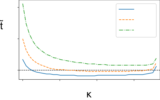
(b)

Figure 10: (a) axial distance $\tilde{s}$ and (b) time $\tilde{t}$ required for 90% (blue), 95% (red), 99% (green) of the particles to focus to the equilibrium for intermediate $\kappa$. The dashed horizontal line indicates the distance and time at which approximately 95% of particles with $15\leq\kappa\leq 25$ are focused.

As $\kappa$ increases the system undergoes saddle-node bifurcation as the stable node and saddle point in each of the upper and lower halves of the duct merge and disappear. Simultaneously a (subcritical) pitchfork bifurcation happens as two saddle points and one stable node on the outer side (right side) merge and become a saddle point (Figure 8). This results in a system with a unique stable equilibrium point that attracts all particles in the duct (Figure 7cd). All equilibria lie on the $\tilde{r}$-axis, due to the vertical reflection symmetry, with the stable node on the inner side (left side) of the duct. Similar to the multi-focus behavior, there exist heteroclinic orbits that connect the saddle to the stable node which act as a slow manifold (Figure 6(b)).

The axial distance and time required for particles to focus on this equilibrium point are important since they determine the length and run time of the apparatus to achieve particle focusing. Technically, if a particle does not start on the stable equilibrium point $(\tilde{r}^{*},\tilde{z}^{*})$ it will take infinite time to arrive at the exact equilibrium point. However, we consider that a particle has “focused” at the equilibrium point if the distance from the particle to the equilibrium is smaller than a certain threshold, which we choose to be $0.01$ for this paper. We define

(13a) $$\tilde{t}^{*}(\tilde{r},\tilde{z}) =\min\big{\{}\tilde{t}:\left\lVert(\tilde{r}_{p},\tilde{z}_{p})(\tilde{t})-(\tilde{r}^{*},\tilde{z}^{*})\right\rVert<0.01,\,(\tilde{r}_{p},\tilde{z}_{p})(0)=(\tilde{r},\tilde{z})\big{\}},$$

(13b) $$\tilde{s}_{p}^{*}(\tilde{r},\tilde{z}) =\tilde{s}_{p}(\tilde{t}^{*}(\tilde{r},\tilde{z})),$$

which correspond to the required time and axial distance for a particle at an initial position $(\tilde{r},\tilde{z})$ in the cross-section to focus. The heat maps in Figure 9ac show, $\tilde{s}_{p}^{*}$ and $\tilde{t}^{*}$ over the cross-section for $\kappa=25$. In each map, black shows the region from which the focusing distance or time is greatest, and dark red shows the region from which the focusing distance or time is shortest.

In order to understand the overall focusing ability in a given axial length or time, we compute the fraction of the channel cross-section area from which particles will have focused in distance $\tilde{s}$ or time $\tilde{t}$. We define these functions $CF_{s}(\tilde{s})$ and $CF_{t}(\tilde{t})$, respectively, as:

(14a) $$CF_{s}(\tilde{s}) =\frac{1}{4}\int_{-1}^{1}\int_{-1}^{1}\scalebox{1.5}{$\chi$}_{\tilde{s}_{p}^{*}\leq\tilde{s}}(\tilde{r},\tilde{z})d\tilde{r}d\tilde{z},$$

(14b) $$CF_{t}(\tilde{t}) =\frac{1}{4}\int_{-1}^{1}\int_{-1}^{1}\scalebox{1.5}{$\chi$}_{\tilde{t}^{*}\leq\tilde{t}}(\tilde{r},\tilde{z})d\tilde{r}d\tilde{z},$$

where $\scalebox{1.5}{$\chi$}_{\tilde{s}_{p}^{*}\leq\tilde{s}}$ and $\scalebox{1.5}{$\chi$}_{\tilde{t}^{*}\leq\tilde{t}}$ are characteristic functions with unit value where $\tilde{s}_{p}^{*}(\tilde{r},\tilde{z})\leq\tilde{s}$ and $\tilde{t}^{*}(\tilde{r},\tilde{z})\leq\tilde{t}$, respectively, and which are zero elsewhere. Assuming that the particles are initially randomly distributed in the cross-section, $CF_{s}$ and $CF_{t}$ give good approximations of the fraction of particles focused after a given distance $\tilde{s}$ and time $\tilde{t}$. Figure 9bd plot $CF_{s}(\tilde{s})$ and $CF_{t}(\tilde{t})$ for $\kappa=25$. We observe that the plots of $CF_{s}$ and $CF_{t}$ are qualitatively similar. This is due to the fact that the change of axial velocity is relatively slow and smooth over the slow manifold.

For engineering design one needs to know the duct length/number of turns of the spiral the duct length required for the majority (e.g. $95\%$) of particles to focus. This corresponds to finding $\tilde{s}$ satisfying $CF_{s}(\tilde{s})=f$, where $f$ is the fraction of particles focused. Figure 10 shows for $10\leq\kappa\leq 28$ the axial distance and time required for $90$, $95$, and $99\%$ of the particles to focus. There is only weak dependence on $\kappa$ for a significant portion of this range. These plots show that a given duct geometry may be used to focus a range of particle sizes. For example, from Figure 10(a), we see that a duct of length $\tilde{s}=300$ will focus at least 95% of particles corresponding to $15\leq\kappa\leq 25$. Once we know the duct length we can estimate how many turns of the spiral required for the focusing. Note that the bend radius is not constant along the spiral however the duct width is much smaller than the bend radius, allowing for small variation in the bend radius in real devices (see e.g. Fig. 1(b)). As an example, using physical parameters in [14, 20] the number of rotations corresponding to $\tilde{s}=300$ is approximately 4 and 1-5, respectively. We note that the duct cross-sections used in the experiments are rectangular rather than square. Still this suggests that only a modest number of turns may be needed to achieve the desired focusing. Then, since the particle radius is $a=G/\kappa^{1/3}$, where $G=(\ell^{4}/4R)^{1/3}$ captures the other geometrical parameters of the duct, at least 95% of all particles of size

$$0.34G\approx G/25^{1/3}\leq a\leq G/15^{1/3}\approx 0.41G$$

will focus after passing through the duct. From Figure 10(b) we see that this focusing takes a time $\tilde{t}\approx 500$. Differences in the size of particles results in different focusing points and, hence, particle separation by size. In practice, there needs to be a significant separation, within the cross section, between focusing positions (as a function of particle size) for effective separation. For example, in Figure 8(a), the variation in the radial coordinate is not large so that separation may be difficult. In general, for square ducts, the focusing position may not have sufficient variation and other cross-sectional shapes may be preferred as discussed in [8]. An analysis similar to this work could be carried out for different cross-sections.

4.3 Periodic orbit behavior (large $\kappa$)

As $\kappa$ increases further, the system undergoes two bifurcations as the stable and unstable nodes on the $\tilde{r}$-axis collide and give birth to an unstable node on either side of the $\tilde{r}$-axis (Figure 11(a)). For $\kappa$ between 25 and 25.5, there exists a vertical pitchfork bifurcation where the unstable node bifurcates to a pair of unstable nodes and a saddle point between them. For $\kappa$ between 27.5 and 28.5, there exists a horizontal saddle-node bifurcation where the saddle point and the stable node cancel out each other. Since ${d\tilde{z_{p}}}/{d\tilde{t}}=0$ on the $\tilde{r}$-axis, the latter bifurcation is determined by ${d\tilde{r_{p}}}/{d\tilde{t}}$ on the axis, which is shown in Figure 11(b). After the two bifurcations occur, there remains two periodic periodic orbits on either side of the $\tilde{r}$-axis, each around one of the unstable nodes (Figure 7e). For $\kappa=30$, the periodic orbits are large with varying particle speeds, slower near the saddle point and where the saddle-node bifurcation occurs. As $\kappa$ increases the periodic orbits become smaller and the particle speed becomes more uniform as they effectively follow the Dean flow (Figure 7f, and 8).

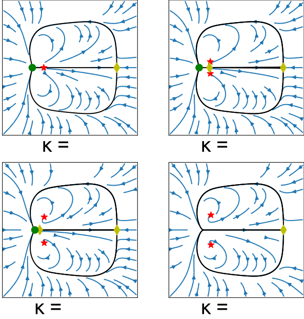
(a) Particle trajectories and equilibria

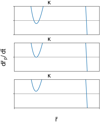
(b) ${d\tilde{r_{p}}}/{d\tilde{t}}$ on the $\tilde{r}$ axis

Figure 11: The two bifurcations between $\kappa=25$ and $30$ within the cross-section, $[-1,1]\crossproduct[-1,1]$. (a) presents the particle trajectories and the equilibria in different colors and shapes: stable nodes (green $\bullet$), saddle points (yellow $\diamondsuit$) and unstable nodes (red $\star$). For $\kappa\leq 28$, the black line represents the heteroclinic orbit that connects the equilibria on the $\tilde{r}$ axis. For $\kappa=28.5$, the black line represents the limit cycle. (b) are graphs of ${d\tilde{r_{p}}}/{d\tilde{t}}$ on the $\tilde{r}$ axis for $28\leq\kappa\leq 28.2$

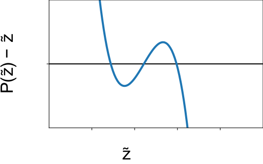
(a) Poincare map for $\kappa$ = 200

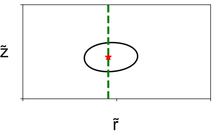
(b) Limit cycle and the manifold

Figure 12: The Poincaré map $P(\tilde{z})$ of the upper half domain, $[-1,1]\crossproduct[0,1]$, for $\kappa=200$. The manifold we choose for the Poincaré map is the vertical line that passes through the unstable nodes (red $\star$) as shown in (b) and (a) is the difference between $\tilde{z}$ and its Poincaré map $P(\tilde{z})$, i.e. $P(\tilde{z})-\tilde{z}$.

These periodic orbits are attractive limit cycles that are unique on each half domain, as shown by calculating the Poincaré map [4]. We choose the manifold that defines the Poincaré map as the vertical line through the unstable equilibrium point in the top half of the duct (Figure 12(b)) and define the Poincaré map $P:(0,1)\rightarrow(0,1)$ taking as input the $\tilde{z}$-coordinate of a particle on the manifold and yielding as output the $\tilde{z}$-coordinate of that particle after a full rotation around the unstable equilibrium. Figure 12(a) shows the $P(\tilde{z})-\tilde{z}$ value for the variable $\tilde{z}$. There are three zeros of the function, the middle one corresponding to the unstable node of the system and the other two corresponding to the limit cycle. The sign on either side of the zeros indicates that this limit cycle is attractive.

4.4 Comparison of ZeLF and detailed numerical models

Figure 13: $\kappa$ values and particle flow behavior of the numerical Model. The flow behavior is classified as described in section 4.4. The different sized circles indicate the four different sized particles from $a=0.05$ to $0.2$. The black line indicates the flow behavior of the ZeLF model. As the size of the particles decrease the behavior matches that of the ZeLF model. Due to the restriction on the range of $R$, the data points of particles with size $a=0.15$ and $0.2$ do not fully extend to exhibit the periodic flow behavior.

Recall that the ZeLF model used for the above analysis is an approximation of the detailed numerical model of [8]. We here compare the predictions of particle dynamics of these two models. From the ZeLF model, we have found that the particle dynamics will differ depending on the value of the parameter $\kappa$. For small $\kappa$ $(\lesssim 10)$ there are multiple points in the duct cross-section to which particles focus depending on their initial position; for intermediate $\kappa$ $(10\lesssim\kappa\lesssim 25$) there is a unique point to which all particles will focus, regardless of their initial position; for large $\kappa$ $(\gtrsim 25)$ there are no stable focus points but particles initially located in the top/bottom half of the duct cross-section will migrate to a periodic orbit in the top/bottom half of the cross-section. Similar changes in particle dynamics are seen using the detailed numerical model but these occur at slightly different values of $\kappa$.

Using a square duct with parameters $l=2$, $80\leq R\leq 5120$ and $a=0.05,0.10,0.15,0.20$, Figure 13 shows the nature of the particle dynamics predicted by the detailed numerical model of [8] for different values of $\kappa$. Also shown, for comparison, are the predictions of the ZeLF model which assumes that the particle size is small compared to the size of the duct ($a\ll\ell$) and that the bend radius $R$ is large ($\epsilon\rightarrow 0$). There is excellent agreement between the ZeLF model and the numerical model for small particle size. As the particle size increases the numerical model gives transitions between the different behaviors at smaller values of $\kappa$, but qualitatively we continue to observe the same three regimes occurring in the same order.

5 Conclusion

Building on previous work [8] we have developed a simplified model for the migration of a small neutrally buoyant particle suspended in relatively slow flow through microfluidic curved ducts with a square cross-section. While curved ducts with a square cross-section are not as effective as rectangular (or other) cross-sections for particle separation by size, they exhibit a wide range of interesting bifurcations. We model the inertial lift force by first fitting the zero level curves to data obtained from simulations of a small particle in a straight duct. Then, multiplying by the exponential of a polynomial in the cross-section coordinates, we fit the inertial lift force over the entire cross-section in a manner that does not modify the zero level curves already modeled. This two-step process is essential to capture the correct topology of the inertial lift force and correctly predict equilibria for large bend radii. To this, we add a simple drag force model to capture the effect of the secondary motion of the background flow. The ratio of the secondary drag to inertial lift forces is parametrized by a single dimensionless variable $\kappa$. Unlike previous studies, we also incorporate travel along the duct into the trajectory model to enable an analysis of the time and distance required for particles to focus.

Using this model we observe that there exist three different $\kappa$ regions with distinctive flow behavior. We introduce a simple criterion to categorize these three $\kappa$ behavior. This categorization aids in identifying appropriate ranges of physical parameters when designing a curved duct for focusing purposes. The methodology and analysis applied to extract and understand the $\kappa$ dependence of the model can be applied to other shaped ducts as well. In addition, we have shown that a duct of a given length will focus particles over a range of $\kappa$ values. This is an important observation as it establishes that a single device design might be used to focus multiple particle sizes simultaneously. Going forwards, it will be interesting to study if this observation holds for non-square ducts and/or non-spherical particles such that the focusing points for particles of different sizes have sufficiently different radial coordinate to enable practical particle separation.

References

- [1] E. S. Asmolov, The inertial lift on a spherical particle in a plane Poiseuille flow at large channel Reynolds number, Journal of Fluid Mechanics, 381 (1999), pp. 63–87, doi.org/10.1017/S0022112098003474.
- [2] D. Di Carlo, Inertial microfluidics, Lab Chip, 9 (2009), pp. 3038–3046, doi.org/10.1039/B912547G.
- [3] T. M. Geislinger and T. Franke, Hydrodynamic lift of vesicles and red blood cells in flow — from Fåhræus and Lindqvist to microfluidic cell sorting, Advances in Colloid and Interface Science, 208 (2014), pp. 161–176, doi.org/10.1016/j.cis.2014.03.002.
- [4] J. Guckenheimer and P. Holmes, Nonlinear oscillations, dynamical systems, and bifurcations of vector fields, vol. 42, Springer Science & Business Media, 2013.
- [5] B. Harding, A study of inertial particle focusing in curved microfluidic ducts with large bend radius and low flow rate, in Proceedings of the 21st Australasian Fluid Mechanics Conference, Adelaide, South Australia, Australia, Australasian Fluid Mechanics Society, December 2018, https://people.eng.unimelb.edu.au/imarusic/proceedings/21/Contribution_603_final.pdf. Contribution number 603.
- [6] B. Harding, A Rayleigh–Ritz method for Navier–Stokes flow through curved ducts, The ANZIAM Journal, 61 (2019), pp. 1–22, https://doi.org/10.1017/S1446181118000287.
- [7] B. Harding and Y. M. Stokes, Inertial focusing of non-neutrally buoyant spherical particles in curved microfluidic ducts, Journal of Fluid Mechanics, (2020), https://doi.org/10.1017/jfm.2020.589.
- [8] B. Harding, Y. M. Stokes, and A. L. Bertozzi, Effect of inertial lift on a spherical particle suspended in flow through a curved duct, Journal of Fluid Mechanics, 875 (2019), pp. 1–43, https://doi.org/10.1017/jfm.2019.323.
- [9] B. P. Ho and L. G. Leal, Inertial migration of rigid spheres in two-dimensional unidirectional flows, Journal of Fluid Mechanics, 65 (1974), pp. 365–400, doi.org/10.1017/S0022112074001431.
- [10] K. Hood, S. Kahkeshani, D. Di Carlo, and M. Roper, Direct measurement of particle inertial migration in rectangular microchannels, Lab on a Chip, 16 (2016), pp. 2840–2850.
- [11] K. Hood, S. Lee, and M. Roper, Inertial migration of a rigid sphere in three-dimensional Poiseuille flow, Journal of Fluid Mechanics, 765 (2015), pp. 452–479, doi.org/10.1017/jfm.2014.739.
- [12] J. M. Martel and M. Toner, Inertial focusing in microfluidics, Annual Review of Biomedical Engineering, 16 (2014), pp. 371–396, doi.org/10.1146/annurev-bioeng-121813-120704.
- [13] J.-P. Matas, J. F. Morris, and É. Guazzelli, Inertial migration of rigid spherical particles in poiseuille flow, Journal of Fluid Mechanics, 515 (2004), pp. 171–195, doi.org/10.1017/S0022112004000254.
- [14] H. Ramachandraiah, H. A. Svahn, and A. Russom, Inertial microfluidics combined with selective cell lysis for high throughput separation of nucleated cells from whole blood, Rsc Advances, 7 (2017), pp. 29505–29514.
- [15] R. Rasooli and B. Cetin, Assessment of lagrangian modeling of particle motion in a spiral microchannel for inertial microfluidics, Micromachines, 9 (2018), p. 433, http://dx.doi.org/10.3390/mi9090433.
- [16] J. A. Schonberg and E. J. Hinch, Inertial migration of a sphere in Poiseuille flow, Journal of Fluid Mechanics, 203 (1989), pp. 517–524, doi.org/10.1017/S0022112089001564.
- [17] G. Segre and A. Silberberg, Radial particle displacements in Poiseuille flow of suspensions, Nature, 189 (1961), pp. 209–210, doi.org/10.1038/189209a0.
- [18] P. Shi and R. Rzehak, Lift forces on solid spherical particles in wall-bounded flows, Chemical Engineering Science, 211 (2020), p. 115264, doi.org/10.1016/j.ces.2019.115264.
- [19] M. E. Warkiani, G. Guan, K. B. Luan, W. C. Lee, A. A. S. Bhagat, P. Kant Chaudhuri, D. S.-W. Tan, W. T. Lim, S. C. Lee, P. C. Y. Chen, C. T. Lim, and J. Han, Slanted spiral microfluidics for the ultra-fast, label-free isolation of circulating tumor cells, Lab Chip, 14 (2014), pp. 128–137, doi.org/10.1039/C3LC50617G.
- [20] M. E. Warkiani, B. L. Khoo, L. Wu, A. K. P. Tay, A. A. S. Bhagat, J. Han, and C. T. Lim, Ultra-fast, label-free isolation of circulating tumor cells from blood using spiral microfluidics, Nature protocols, 11 (2016), pp. 134–148.