Distinguishing gravitational and emission physics in black-hole imaging: spherical symmetry

Abstract

Imaging a supermassive black hole and extracting physical information requires good knowledge of both the gravitational and the astrophysical conditions near the black hole. When the geometrical properties of the black hole are well understood, extracting information on the emission properties is possible. Similarly, when the emission properties are well understood, extracting information on the black-hole geometry is possible. At present however, uncertainties are present both in the geometry and in the emission, and this inevitably leads to degeneracies in the interpretation of the observations. We explore here the impact of varying geometry and emission coefficient when modelling the imaging of a spherically-accreting black hole. Adopting the Rezzolla-Zhidenko parametric metric to model arbitrary static black-holes, we first demonstrate how shadow-size measurements leave degeneracies in the multidimensional space of metric-deviation parameters, even in the limit of infinite-precision measurements. Then, at finite precision, we show that these degenerate regions can be constrained when multiple pieces of information, such as the shadow-size and the peak image intensity contrast, are combined. Such degeneracies can potentially be eliminated with measurements at increased angular-resolution and flux-sensitivity. While our approach is restricted to spherical symmetry and hence idealised, we expect our results to hold also when more complex geometries and emission processes are considered.

1 Introduction

The characteristic central brightness depression in the first Event Horizon Telescope (EHT) image of M87^∗ provides strong evidence of its nature as a supermassive black hole (BH; Event Horizon Telescope Collaboration et al. 2019a, b, c, d, e, f). The size of the narrow, bright ring in the observed image sets an upper bound on the size of the central dark compact object. By comparing the observed image against a large library of synthetic images obtained from general-relativistic radiative-transfer (GRRT) computations coupled to general-relativistic magnetohydrodynamics (GRMHD) simulations of Kerr BHs being orbited by a turbulent, hot, magnetized disk in general relativity (GR; Event Horizon Telescope Collaboration et al. 2019d, e), the angular gravitational radius $\theta_{\text{g}}=GM/c^{2}D$ of M87^∗ can be ascertained, with $M$ its mass and $D$ the distance to it. The consistency of this value obtained by the EHT with the one obtained previously from stellar-dynamics measurements (Gebhardt et al., 2011) demonstrates that GR passes the null-hypothesis test (Event Horizon Telescope Collaboration et al., 2019f).

The width of the posterior on the fractional difference between these two measurements of $\theta_{\text{g}}$ can be used to infer crucial, albeit approximate, bounds on the size of the shadow of M87^∗. Furthermore, while all BHs cast shadows, there exist other compact objects (or black-hole mimickers), e.g., horizonless compact objects, both with and without singularities, wormholes, etc., that can be used to model the observed image of M87^∗ (see, e.g., Kocherlakota & Rezzolla 2020). Besides testing what type of exotic object M87^∗ is, there are also theory-specific possibilities that one can test for indirectly by considering whether the EHT image is consistent with the BH solutions from those theories. The latter include looking for the existence of additional matter fields, conspicuous in the strong gravitational fields around BHs (such as the axion in Sen 1992), anomalous couplings between gravity and/or fields, possibly leading to violations of the Einstein equivalence principle (Gibbons & Maeda, 1988), etc. Such a comparison, using the EHT shadow-size constraints, considering various well-known BH and non-BH solutions from GR and alternative theories has recently been reported in Kocherlakota et al. (2021). An accurate quantification of the size of deviation of these solutions from the Schwarzschild solution may be found in Kocherlakota & Rezzolla (2020).

While such analyses (Psaltis et al., 2020; Kocherlakota et al., 2021; Völkel et al., 2021) make use solely of the shadow-size constraints, the measurements in reality contain additional potentially useful information. Barring a few recent studies (Broderick et al., 2014; Johannsen et al., 2016; Mizuno et al., 2018; Olivares et al., 2020), the dearth of simulations of accreting non-Kerr BH and non-BH spacetimes, and of the associated analyses that would identify and extract novel features that they may present, limits the present ability to distinguish BHs of various theories. Notwithstanding the computational costs and the conceptual hurdles involved in expanding the presently available body of GRRT and GRMHD codes to accommodate non-Maxwell and non-Einstein-Hilbert theories respectively, it is presently unclear whether this is the most effective route at the moment.

Thus, proposing and developing semi-analytical accretion and emission models (Bambi & Modesto, 2013; Younsi et al., 2016; Pu & Broderick, 2018; Shaikh et al., 2019; Gimeno-Soler et al., 2019; Shaikh & Joshi, 2019; Narayan et al., 2019; Gan et al., 2021; Yang et al., 2021), and studying the variation of image features with these models and with varying spacetime geometry, as a path-finding step, could already yield important insights. Such analyses require fewer expensive operations such as integrations, and greatly reduce the overall computational cost, enabling a broader parameter survey. This is the logic followed in this work, where we adopt a generic but rapidly converging parameterisation of spherically symmetric BHs via the Rezzolla-Zhidenko (RZ) expansion (Rezzolla & Zhidenko, 2014), and a series of simple but effective spherically symmetric emission models. Furthermore, in addition to the shadow-size bounds, we also use (a) the scaling parameter $\alpha=d/\theta_{\text{g}}$ of the angular diameter $d$ of the observed ring feature in the M87^∗ image with its angular gravitational radius, (b) the lower bound on the maximum contrast in the image $\mathcal{C}_{\text{peak, EHT-min}}$, and (c) the fractional-width of the ring $f_{\text{w}}$, inferred by the EHT (see Table 1 of Event Horizon Telescope Collaboration et al. 2019a).

Adopting this approach, it then becomes possible to address, albeit within the present context of spherical models, some of the concerns that have recently been raised, e.g., in Gralla (2021), about the location of peak of emission near M87^∗, when modelled as a Schwarzschild BH, namely whether it is closer to the location of the innermost stable circular orbit or the photon sphere. We can also identify certain characteristic features in the observed image that are reasonably robust against varying emission prescriptions, such as the location of the peak contrast in the observed image and some that are not (value of peak contrast, fractional ring width, etc.). Indeed, it can be argued that this latter set of observables can be used to gain insight into the emission physics near accreting supermassive BHs. In this sense, recent work has considered the use of principal-component analyses to use all of the information in the image (see, e.g., Medeiros et al. 2020; Lara et al. 2021).

More importantly, the work reported here can be used to determine which degeneracies may emerge when distinguishing gravitational and emission physics in BH imaging. It is clear, in fact, that extracting physical information from a supermassive BH image requires a good knowledge of both the gravitational and astrophysical conditions near the black hole. The uncertainties associated with the spacetime geometry and with the emission mechanisms, and which are presently still rather large, inevitably lead to degeneracies in the interpretation of the observations. Indeed, while the EHT shadow-size measurements already impose non-trivial constraints on the relevant parameter space of any family of BHs, it is in general extremely difficult to distinguish – even in the limit of a perfectly precise measurement – BHs which belong to a two-parameter family that have differing horizon-sizes but which predict identical shadow-sizes (see the top row of Fig. 4). This limitation, however, is simply due to the use of a single observable: the shadow-size (see, e.g., Völkel et al. 2021). Hence, complementing the latter with the location of the observed peak of emission (characterized by $\alpha$) drastically changes the scenario, and it is therefore possible, in principle, to isolate the relevant metric parameters (see the bottom row of Fig. 4). We also illustrate that ever more detailed descriptions of the spacetime geometry, which emerge when considering BHs described by three independent parameters, bring in additional degeneracies. These, however, can be further resolved by exploiting other observables such as precise measurements of the fractional-width of the observed bright ring or with future observables such as the sizes of photon subrings that the next-generation EHT (ngEHT) hopes to observe (Gralla et al. 2019; Johnson et al. 2020; Broderick et al. 2021).

The structure of the paper is as follows. In Sec. 2 we summarise the simple radially freely infalling accretion model that we will use exclusively here, and discuss also a prescription for the associated emission that naturally follows (see Narayan et al. 2019). In Sec. 3, keeping the spacetime geometry fixed to that of a Schwarzschild BH, we compare the observed contrast profiles obtained by applying the aforementioned accretion-emission model against those obtained from other emission models that are currently in use. We also introduce an artificial inner cut-off for the emitting region as a simplistic proxy for a peaked emission profile and study how this impacts the final image. In Sec. 4, we vary the spacetime metric when using two characteristic emission prescriptions, and explore the constraints imposed by the EHT measurements on the space of parameters that induce deviations from the Schwarzschild geometry. In Sec. 5, we characterise the ring widths of the emission rings around various RZ BHs for different emission models and show that the shadow boundary always forms the inner edge of the emission ring, independently of whether or not there is an inner cutoff in the emission zone outside the horizon.

The purpose of the present work is to demonstrate, using spherically symmetric geometry and emission, that is possible to test the nature of strong gravitational fields near supermassive compact objects with the EHT. We expect that much of what discussed here will continue to hold also when more realistic emission models, such as those considered in Event Horizon Telescope Collaboration et al. (2019e) and Event Horizon Telescope Collaboration et al. (2019f), would be used in conjunction with axisymmetric spacetimes (Konoplya et al., 2016).

2 Spherical Accretion and Emission Models

In what follows, we will assume that photons and accreting material moves on geodesics of the spacetime metric. Further, the symbol $\nu$ and the index $\nu$ will be used to denote frequencies and specific quantities; Thus, e.g., $I_{\nu}$ will be the specific intensity and is a scalar quantity.

The line-element describing the exterior geometry of an arbitrary static BH can be written, in areal-polar coordinates $x^{\alpha}=(t,r,\theta,\phi)$, as,

$$ds^{2}=g_{\alpha\beta}dx^{\alpha}dx^{\beta}=-N^{2}(r)dt^{2}+\frac{B^{2}(r)}{N^{2}(r)}dr^{2}+r^{2}d\Omega_{2}^{2}\,,$$ (1)

where $d\Omega_{2}^{2}:=d\theta^{2}+\sin^{2}\theta~{}d\phi^{2}$ is the standard line-element on the two-sphere.

Due to the existence of the Killing vectors $\partial_{t}$ and $\partial_{\phi}$ in such a spacetime (Eq. 1), there exist a pair of associated conserved quantities, $E$ and $L$, along every geodesic, $x^{\alpha}(\lambda)$. These can be obtained straightforwardly from the Lagrangian for geodesic motion, $2\mathscr{L}:=g_{\alpha\beta}\dot{x}^{\alpha}\dot{x}^{\beta}$, as,

$$-E:= \ p_{t}=\partial_{\dot{t}}\mathscr{L}=-N^{2}\dot{t}\,,$$ (2)

$$L:= \ p_{\phi}=\partial_{\dot{\phi}}\mathscr{L}=r^{2}\sin^{2}\theta\dot{\phi}\,,$$

where the overdot denotes a derivative with respect to the affine parameter $\lambda$ along the geodesic. The Lagrangian $\mathscr{L}$ is itself also a conserved quantity along a geodesic ($2\mathscr{L}=0,-1$ for null and timelike geodesics), and when rewritten in terms of the other conserved quantities, as,

$$2\mathscr{L}=-\frac{E^{2}}{N^{2}}+\frac{B^{2}}{N^{2}}\dot{r}^{2}+r^{2}\dot{\theta}^{2}+\frac{L^{2}}{r^{2}\sin^{2}\theta}\,,$$ (3)

yields a separable equation for the radial and the polar velocity components,

$$0=\left(\frac{r^{2}B^{2}}{N^{2}}\frac{\dot{r}^{2}}{E^{2}}-\frac{r^{2}}{N^{2}}-\frac{2\mathscr{L}r^{2}}{E^{2}}\right)+\left(r^{4}\frac{\dot{\theta}^{2}}{E^{2}}+\frac{L^{2}}{E^{2}}\csc^{2}\theta\right)\,.$$

The existence of a fourth conserved quantity, called the Carter constant $C$, associated with the existence of an additional “hidden” symmetry and characterized by the Killing-Yano tensor (see, e.g., Hioki & Maeda 2009; Abdujabbarov et al. 2015) allows for us to write, with $\xi:=L/E$ and $\mathscr{I}:=C/E^{2}+\xi^{2}$,

$$\frac{\dot{r}^{2}}{E^{2}}= \ \frac{1+2\mathscr{L}E^{-2}N^{2}-\mathscr{I}r^{-2}N^{2}}{B^{2}}:=V_{\text{r}}(r)\,,$$ (4)

$$\frac{\dot{\theta}^{2}}{E^{2}}= \ \frac{\mathscr{I}-\xi^{2}\csc^{2}\theta}{r^{4}}\,.$$

Thus the four-velocity along an arbitrary geodesic $x^{\alpha}(\lambda)$ with conserved quantities $\left\{E,\xi,\mathscr{L},\mathscr{I}\right\}$ is given as,

$$\frac{\dot{x}_{\pm,\pm}^{\alpha}}{E}= \ \left(\frac{1}{N^{2}},\pm\frac{\left[1+2\mathscr{L}E^{-2}N^{2}-\mathscr{I}r^{-2}N^{2}\right]^{1/2}}{B}\right.\,,$$ (5)

$$\ \left.\pm\frac{\sqrt{\mathscr{I}-\xi^{2}\csc^{2}\theta}}{r^{2}},\frac{\xi}{r^{2}\sin^{2}\theta}\right)\,,$$

where the indices $\pm,\pm$ above correspond to the sign of the radial and polar velocities respectively.

2.1 Spherical Accretion Model and Observed Intensity Profile

The spherical accretion model of interest here is that of a fluid in radial free-fall towards the central compact object. The four-velocity $u^{\alpha}_{\text{e}}$ along such a radially freely infalling ($d\Omega_{2}=0$) timelike emitter is [see Eq. (5)],

$$u_{\text{e}}^{\alpha}=\bar{E}\left(\frac{1}{N^{2}},-\frac{\sqrt{1-\bar{E}^{-2}N^{2}}}{B},0,0\right)\,,$$ (6)

where $\bar{E}$ is the energy per unit mass of a fluid element at infinity.

As is reasonable, we will restrict to the case when the fluid elements have negligible (radial) kinetic energy at infinity (i.e., $\lim_{r\rightarrow\infty}u^{r}_{\text{e}}\simeq 0$ or $\bar{E}\simeq 1$). Further, the four-velocity $u^{\alpha}_{\text{o}}$ of an asymptotic static observer ($d\Omega_{2}=dr=0$) is,

$$u_{\text{o}}^{\alpha}=\lim_{r\rightarrow\infty}\left(N^{-1},0,0,0\right)=(1,0,0,0)\,.$$ (7)

A photon that is emitted at a radius $r$ with an emitter-frame frequency of $\nu_{\text{e}}$ appears in the frame of the observer to be of frequency $\nu_{\text{o}}$, due to gravitational and Doppler redshift. This redshift factor $\gamma_{\pm}$ for radially-outgoing (+) and -ingoing (-) photons is then given as,

$$\gamma_{\pm}(r)=\frac{\nu_{\text{o}}}{\nu_{\text{e}}}=\frac{\left(k_{\pm,\pm}\right)_{\alpha}u^{\alpha}_{\text{o}}}{\left(k_{\pm,\pm}\right)_{\beta}u^{\beta}_{\text{e}}}\simeq\frac{N^{2}}{1\pm\sqrt{\left(1-\mathscr{I}r^{-2}N^{2}\right)\left(1-N^{2}\right)}}\,,$$ (8)

where in writing the last relation above we have used $\bar{E}\approx 1$, and $k^{\mu}_{\pm,\pm}$ denotes the four-velocity of a photon [see Eq. (5)],

$$k_{\pm,\pm}^{\mu}=E\left(\frac{1}{N^{2}},\pm\frac{\sqrt{1-\mathscr{I}r^{-2}N^{2}}}{B},\pm\frac{\sqrt{\mathscr{I}-\xi^{2}\csc^{2}\theta}}{r^{2}},\frac{\xi}{r^{2}\sin^{2}\theta}\right)\,,$$

Notice that due to the purely radial motion of the emitter [see Eq. (6)] the redshift experienced by a photon is independent of its polar $(k_{\pm,\pm}^{\theta})$ and azimuthal $(k^{\phi})$ velocities, thus removing all $\theta$-dependence.

In general, in the presence of a fluid that both emits and absorbs radiation, the covariant radiative-transfer equation, written in the local fluid-frame, reads (see, e.g., Younsi et al. 2012),

$$\frac{dI_{\nu}}{d\lambda}=-\left(k_{\pm,\pm}\right)_{\beta}u_{\text{e}}^{\beta}\left(-q_{\nu}I_{\nu}+\frac{j_{\nu}}{\nu^{3}}\right)\,,$$ (9)

where $I_{\nu}$ is the specific intensity of a ray at frequency $\nu$, and $q_{\nu}$ and $j_{\nu}$ are the absorption and emission coefficients at that frequency respectively. Here however, as is relevant for the observing frequency of the EHT, we will consider the scenario of an optically-transparent fluid ($q_{\nu}=0$) that emits isotropically and monochromatically in its rest frame, $j_{\nu}=\delta(\nu-\nu_{\star})j$. For this scenario, the total intensity $I$ at a location $(\alpha,\beta)$ on the observer’s celestial plane is given as (see, e.g., Sec. 2.3 of Jaroszynski & Kurpiewski 1997; See also Bambi 2013; Shaikh et al. 2019),

$$I(\alpha,\beta)=-\fint\int\gamma_{\pm}^{4}\left(k_{\pm,\pm}\right)_{\beta}u_{\text{e}}^{\beta}j_{\nu}~{}\text{d}\lambda~{}\text{d}\nu=\fint\gamma_{\pm}^{3}j\frac{\text{d}r}{k_{\pm,\pm}^{r}}\,,$$ (10)

where the slash indicates that the integral is evaluated along the full inextensible worldline, through the emitting fluid, of the photons that appear in the observer’s sky at $(\alpha,\beta)$, and the sign of the redshift factor is chosen depending on whether the photon velocity is locally directed radially-outward ($+$) or -inward ($-$). The Cartesian celestial coordinates $(\alpha,\beta)$ on the sky of an asymptotic static observer, inclined at an angle $\theta_{\text{o}}$ with respect to the BH’s (positive) $z$-axis, that were introduced above can be related to the conserved quantities of the photons that appear there via (Bardeen, 1974; Hioki & Maeda, 2009),

$$\left(\alpha,\beta_{\pm}\right):=\left(-\xi\csc{\theta_{\text{o}}}\,,\pm\sqrt{\mathscr{I}-\xi^{2}\csc^{2}{\theta_{\text{o}}}}\right)\,,$$ (11)

with the sign determined by the polarity of its polar velocity.

From Eq. (10) we see that the inclination angle of the observer $\theta_{\text{o}}$ does not impact image formation in this simplified spherical accretion and emission setup; i.e., the only combination of $(\alpha,\beta)$ in the above is $\alpha^{2}+\beta^{2}=\mathscr{I}$, and the final image is circularly symmetric on the observer’s celestial plane. These properties greatly simplify the image construction, and we can simply compute the integral above (Eq. 10) along the the $x$-axis of the image plane for an equatorial asymptotic observer w.l.g., i.e., for $\theta_{\text{o}}=\pi/2$ and $\beta=0$, and simply rotate $\mathit{I}(\alpha\!=\!\xi,\beta\!=\!0):=I(\xi)$ to obtain the full 2-d intensity profile, $\mathit{I}(\alpha,\beta)$. Therefore, the integral we will be concerned with is,

$$\mathit{I}(\xi)=\begin{cases}\int_{r_{\text{cut}}}^{\infty}\gamma_{+}^{3}~{}j~{}\Lambda~{}\text{d}r\,,&|\xi|<\xi_{\text{ps}}\\ \int_{\max{\{r_{\text{cut}},r^{+}_{\text{ps}}\}}}^{\infty}\gamma_{+}^{3}~{}j~{}\Lambda~{}\text{d}r\,,&|\xi|=\xi_{\text{ps}}\\ \int_{\max{\{r_{\text{cut}},r_{\text{tp}}(\xi)\}}}^{\infty}\left(\gamma_{-}^{3}+\gamma_{+}^{3}\right)~{}j~{}\Lambda~{}\text{d}r\,,&|\xi|>\xi_{\text{ps}}\,,\end{cases}$$ (12)

where $r=r_{\text{cut}}\geq r_{0}$ is the location of the inner edge of the emission zone, where $r_{0}$ denotes the location of the outermost Killing horizon, $\Lambda:=|1/k_{\pm,\pm}^{r}|$, $\xi=\xi_{\text{ps}}$ is the impact factor of a photon moving on the photon sphere which is located at $r=r_{\text{ps}}$ (the superscript $+$ denotes an infinitesimally larger value), and $r=r_{\text{tp}}(\xi)$ is the location of the (radial) turning point of a photon with an impact factor of $\xi$ (see Sec. 2.2 below).

Although the existence of a such a sharp inner edge of emission is highly unrealistic, we employ $r_{\text{cut}}$ here as a proxy to study the impact of severe emission suppression close to the event horizon on the final image. Alternatively, and possibly more reasonably, $r=r_{\text{cut}}$ can be thought of as representing the location of the surface of a hypothetical exotic compact object such as a gravastar (see, e.g., Mazur & Mottola 2004), whose size we can then potentially constrain.

2.2 Radial Turning Points of Null Geodesics and the Photon Sphere

The (radial) turning point of an equatorial photon ($\theta=\pi/2$; $\mathscr{I}=\xi^{2}$) is defined as the location where its radial velocity changes sign, i.e., $\dot{r}=0$, which implicitly determines its radial coordinate $r=r_{\text{tp}}(\xi)$ as a function of its impact factor $\xi$,

$$r_{\text{tp}}(\xi)=\xi N(r_{\text{tp}}(\xi))\,.$$ (13)

Equivalently, we can write the impact factor of a photon that has a radial turning point at a coordinate $r$ from the inverse relation, $\xi_{\text{tp}}(r):=r/N(r)$.

For the special case of a photon on an equatorial circular null geodesic (CNG), $\dot{r}=\ddot{r}=0$, we require additionally that,

$$r\partial_{r}N-N=0\,.$$ (14)

If the equation above has a single root, and the CNG is unstable to radial perturbations ($\partial^{2}_{r}V_{\text{r}}<0$), then it locates the photon sphere, $r=r_{\text{ps}}$, in the spacetime. The associated impact factor $\xi=\xi_{\text{ps}}$ of a photon on such an orbit corresponds to the size of the shadow as seen by an asymptotic observer [Eq. (13)],

$$\xi_{\text{ps}}=r_{\text{ps}}/N\left(r_{\text{ps}}\right)\,.$$ (15)

Therefore, in writing the total intensity integral above (Eq. 12) for photons with $|\xi|>\xi_{\text{ps}}$, we have just explicitly split the integral into the parts corresponding to the ingoing and outgoing pieces of the photon orbit respectively. Furthermore, the piecewise definition of the integral above (Eq. 12) becomes clear when remembering that photons with $|\xi|<\xi_{\text{ps}}$ do not turn: these are either ingoing and are captured by the BH at the photon sphere, or are outgoing and reach asymptotic infinity. Of course, the latter set of photons can be sourced only outside the outermost Killing horizon (see also Appendix A for a graphical representation of the radial orbits of null geodesics in the Schwarzschild BH spacetime)

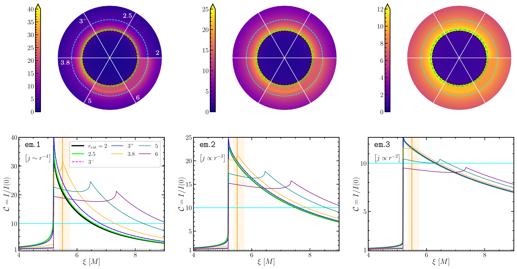
Figure 1: In the top row we show the variation, on the celestial plane of an asymptotic observer, of the contrast in the images of Schwarzschild BHs that are undergoing spherical accretion. In each panel, we keep the isotropic, monochromatic emission prescription $j$ unchanged but vary the inner boundary of emitting region $r_{\text{cut}}$ across sextants, as indicated in the top left panel. We also mark the impact factors of photons that “turn” at the photon sphere $r=3M$ (black circle), $r=3.8M$ (lime; corresponding to an impact factor of $\xi_{\text{peak; EHT}}\approx 5.5M$), and at the ISCO $r=6M$ (cyan), for reference. The characteristic central contrast depression, seen in all the images as a violet disk, is bounded precisely by the black circle. In the bottom row, we show a one-dimensional cut of all of the sextants from the figure above in different colours as indicated in the bottom left panel. While the horizontal cyan line marks the lower bound of the maximum-contrast as measured by the EHT for M87^∗ $C_{\text{peak, EHT-min}}$, the vertical orange line marks the approximate location of the peak of emission $\xi_{\text{peak; EHT}}$, with the orange band around it representing the error in the same. Finally, across columns, we run over the emission models tabled in Table 1, to study the impact of $j$ on the observed image. All radii in the figure are reported in units of the BH ADM mass $M$. Notice also that these figures plots are independent of the value of the constant mass accretion rate $\dot{m}_{\infty}$ since the contrast is a ratio of intensities.

2.3 Emission Coefficient

Thus far we have left the spacetime and the radial variation of the emission coefficient unfixed. Here we show how adopting a constant mass accretion rate $\dot{m}_{\infty}$ for the spherical accretion process described above automatically yields one prescription for the emission coefficient $j$, as in Narayan et al. (2019).

An infinitesimal fluid element of mass $dm$ with an energy per unit mass at infinity $\bar{E}=1$ (i.e., at rest at infinity) that free-falls radially inwards converting gradually its potential energy into kinetic energy. The fluid element then comes to rest at a radius $r$, where it loses its kinetic energy releasing a maximum energy in radiation $\bar{E}_{\text{emit}}$ in radiation corresponding to the difference in its binding energy [see Eq. (7)]

$$E_{\text{emit}}(r)=dm\left(\bar{E}-\bar{E}(r)\right)=dm\left(1-N(r)\right)\,.$$ (16)

Thus, the net emitted luminosity $L$ ($\text{erg}~{}\text{s}^{-1}$) in this scenario, as measured at infinity, is given as, $L(r)=\dot{m}_{\infty}E_{\text{emit}}$, from which we can infer the isotropic specific emission coefficient $j_{\nu}$ ($\text{erg}~{}\text{s}^{-1}\text{cm}^{-3}\text{ster}^{-1}\text{Hz}^{-1}$) in the proper frame of the fluid using the relation,

$$L(r)=\int_{r}^{\infty}\int_{0}^{2\pi}\int_{0}^{\pi}\int_{\nu}\sqrt{-|g|}\sqrt{-g_{tt}}4\pi~{}j_{\nu}~{}\text{d}r^{\prime}~{}\text{d}\phi~{}\text{d}\theta~{}\text{d}\nu\,,$$

where $|g|$ is the determinant of the metric. For monochromatic, isotropic emission in the rest frame,

$$j(r)=\ -\frac{\partial_{r}L}{16\pi^{2}r^{2}BN}=\frac{\dot{m}_{\infty}\partial_{r}N}{16\pi^{2}r^{2}BN}\,.$$ (17)

For such emission around a Schwarzschild BH, we can write,

$$j_{\text{Schw}}(r)=\frac{\dot{m}_{\infty}}{16\pi^{2}r^{3}(r-2M)}\,.$$ (18)

The large-$r$ ($r\gtrsim 3M$) approximation for the maximum emitted energy in a Schwarzschild spacetime reads, from Eq. 16,

$$E_{\text{emit}}=dm\left(1-\sqrt{1-\frac{2M}{r}}\right)\approx\frac{dm~{}M}{r}\,.$$ (19)

This is equivalent to Eq. (12) of Narayan et al. (2019), from which we can also obtain their emission coefficient, given in Eq. (11) of the same paper.

3 Variation of Observed Ring Size with Emission Model: Schwarzschild black hole

Here we fix the spacetime metric to that of a Schwarzschild BH $(N^{2}=1-2M/r;B^{2}=1)$, and study the impact of varying the emission coefficient $j$ and the inner cut-off of the emission region, $r_{\text{cut}}$, on the final image. We summarise the various emission prescriptions that we will use in this section in Table 1, and report the observed contrast profile, $\mathcal{C}(\xi)=\mathit{I}(\xi)/\mathit{I}(0)$, for each model in Fig. 1.

Table 1: We compile below the different models we use to construct the images of a Schwarzschild BH undergoing spherical accretion, displayed in Fig. 1. We have used $k_{3}$ and $k_{2}$ to represent arbitrary constants.

Model	Emissivity model	Reference
em.1	$j={\dot{m}_{\infty}}/{16\pi^{2}r^{3}(r-2M)}$	Eq. (18)
em.2	$j=k_{3}r^{-3}$	Jusufi et al. (2021)
em.3	$j=k_{2}r^{-2}$	Bambi (2013)

Independently of the emission model $j$ and of an inner emission region cutoff at $r=r_{\text{cut}}$, we find an invariably sharp drop in contrast at the shadow boundary, $\xi=\xi_{\text{ps}}=3\sqrt{3}M$, already evident from Eq. 12. The primary role of the emission coefficient is in determining the rate of decay of the intensity with increasing $\xi$, and thus determines the width of the observed emission ring, defined using the locations of the maximum and the half-maximum intensities. Imposing a cut-off in the emission inside the photon sphere $r_{0}<r_{\text{cut}}\leq r_{\text{ps}}$ modifies the intensity inside the shadow boundary $|\xi|<\xi_{\text{ps}}$, and thus the overall contrast profile slightly. However, the peak in the observed contrast profile remains at the shadow boundary $\xi_{\text{peak}}=\xi_{\text{ps}}$, with its value remaining divergent $\mathcal{C}_{\text{peak}}:=\mathcal{C}(\xi_{\text{peak}})=\infty$. On imposing an artificial cut-off at a larger radius $r_{\text{cut}}>r_{\text{ps}}$ we find that the peak of the observed contrast profile shifts to $\xi_{\text{peak}}=\xi_{\text{tp}}(r_{\text{cut}})$, i.e., to the impact factor of the photon that “turns” at $r=r_{\text{cut}}$ (see below Eq. 13), as is expected from Eq. (12). We also find a drop in the maximum contrast in the image, which becomes finite, and decreases with increasing $r_{\text{cut}}$. Furthermore, the value of the contrast at a fixed radius on the observer’s sky, e.g., at $\xi=\xi_{0}$ increases with increasing $r_{\text{cut}}$ until $r_{\text{cut}}=r_{\text{tp}}(\xi_{0})$, after which it starts decreasing (see Sec. 5 for further details). Finally, we note that the observed location and the magnitude of peak of the contrast in the image can be compared against EHT data to obtain constraints on the emission models used here. While we discuss the results one may derive from such an exercise below for demonstrative purposes, it is important to note here that (a) the properties of the accretion flow around astrophysical BHs, such as M87^∗ and Sgr A^∗, are expected to be qualitatively different, best modelled by radiatively inefficient accretion flows (RIAFs; Yuan & Narayan 2014), and (b) the $\alpha$-measurement we use below depends critically on the measurement of $\theta_{\text{g}}$, via a calibration of EHT data against the EHT synthetic image library, the latter having been constructed from simulations of RIAFs around the Kerr BHs of GR.

Indeed, the EHT has reported a measurement for the scaling $\alpha$ of the angular diameter of the observed bright ring $d$ in the image of M87^∗ in terms of its angular gravitational radius $\theta_{\text{g}}$, as $\alpha=d/\theta_{\text{g}}=11^{+0.5}_{-0.3}$ (Table 1 of Event Horizon Telescope Collaboration et al. 2019a), along with a lower-bound on the maximum observed contrast $C_{\text{peak, EHT-min}}\gtrsim 10$. We use the former measurement, i.e., $\xi_{{\text{peak, }}{\text{\tiny{EHT}}}}/M:=\alpha/2\approx 5.5$ to find that the location of the peak of emission in the spacetime must be approximately at $r_{\text{cut}}\approx 3.77M$, for the Schwarzschild BH in the present accretion-emission setup. Using the $1\!-\!\sigma$ values leads to a $10\%$ variation at the most. As can be seen from Eq. 12 and Fig. 1, this is independent of the emission models we use here. At the same time, it is important to note that the maximum contrast in the image $\mathcal{C}_{\text{peak}}:=\mathcal{C}(\xi=\xi_{\text{peak}})$ varies with $j$; In particular, if we write it as $j=k_{n}r^{-n}$ ($k_{n}$ representing a constant), then, as expected, steeper emission coefficients (larger $n$) yield larger $\mathcal{C}_{\text{peak}}$. We refer the reader to see Sec. 5 for further details. Thus, we are in broad agreement with the results of the EHT, despite the accretion model being drastically different, that the peak in emission occurs quite close to the photon sphere. To compare, the impact parameter of a photon that has a turning point at the location of the Schwarzschild innermost stable circular orbit (ISCO) is $\xi_{\text{tp}}(r_{\text{ISCO}}=6M)=\sqrt{54}M$, which implies that if the peak of emission in the spacetime were located instead at the ISCO, the radius of the observed ring in the image would be about $34\%$ larger than the fiducial value of $\xi_{{\text{peak, }}{\text{\tiny{EHT}}}}$ that we have adopted here.

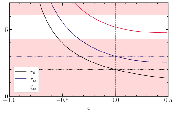
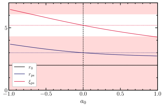
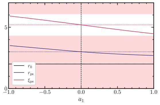
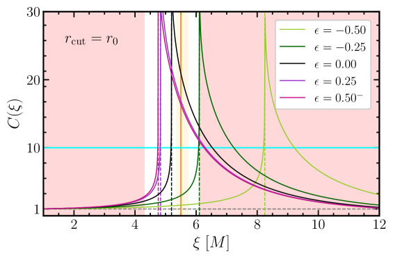
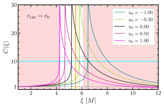
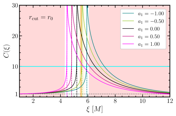
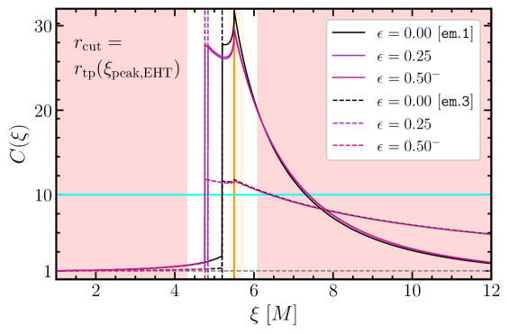
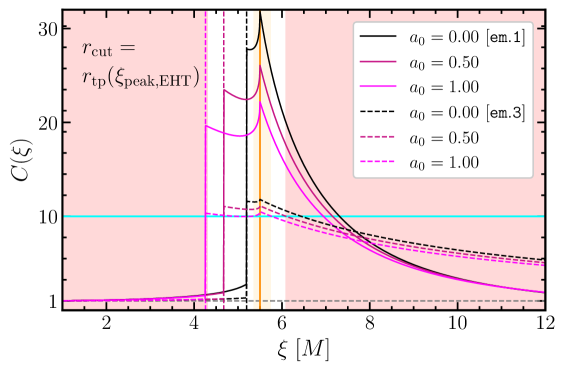
Figure 2: In the top row, we show the variation in the sizes of the event horizon $r_{0}$, the photon sphere $r_{\text{ps}}$, and the shadow $\xi_{\text{ps}}$, with the relevant metric parameter for the single-parameter RZ BHs we use here. In the middle row, we display the contrast profile $\mathcal{C}(\xi)$, as seen on the observer’s sky, when the emission region extends all the way down to the BH event horizon. The bottom row shows the contrast profiles of the set of BHs that have $\xi_{\text{ps}}<\xi_{{\text{peak, }}{\text{\tiny{EHT}}}}$ with an imposed inner cut-off for the emission region at $r_{\text{cut}}=r_{\text{tp}}(\xi_{{\text{peak, }}{\text{\tiny{EHT}}}})$, so that the location of the peak in the contrast profile is at the EHT reported value. The red region in all panels shows the range of parameter disallowed by the EHT-reported shadow-size constraints. The vertical orange line corresponds to $\xi=\xi_{{\text{peak, }}{\text{\tiny{EHT}}}}$, and the orange band shows the associated $1\!-\!\sigma$ range. The horizontal cyan line is the lower bound for $\mathcal{C}_{\text{peak, EHT}}$ reported by the EHT.

Table 2: We show here the theoretically-allowed parameter ranges for various sections of the $\mathscr{M}(\epsilon;a_{0};a_{1})$ RZ BHs we consider here. We also show which PN parameters vanish in general in each case, and when the horizon size is identical to that of a Schwarzschild BH, $r_{0}=2M$.

Model	RZ Parameters: Theoretically-Allowed Range			PN Parameters			$r_{0}=2M$
	$\epsilon$	$a_{0}$	$a_{1}$	$\zeta_{1}$	$\zeta_{2}$	$\zeta_{3}$
$\mathscr{M}(\epsilon)$	$-1<\epsilon\leq 1/2$	0	0	0	$\neq 0$	0	$\times$
$\mathscr{M}(a_{0})$	0	$a_{0}\geq-1$	0	$\neq 0$	$\neq 0$	0	$\checkmark$
$\mathscr{M}(a_{1})$	0	0	$a_{1}\geq-1$	0	$\neq 0$	$\neq 0$	$\checkmark$
$\mathscr{M}(a_{0};a_{1})$	0	$a_{0}\leq-3$	$a_{1}\geq\frac{2\sqrt{-a_{0}^{3}}}{3\sqrt{3}}$	$\neq 0$	$\neq 0$	$\neq 0$	$\checkmark$
		$a_{0}>-3$	$a_{1}\geq-1-a_{0}$
$\mathscr{M}(\epsilon;a_{1})$	$-1<\epsilon\leq 1$	0	$a_{1}\geq-1+2\epsilon$	0	$\neq 0$	$\neq 0$	$\times$
	$\epsilon>1$		$\displaystyle a_{1}\geq\frac{1}{27}\left[9\epsilon^{2}+2\epsilon^{3}+2\sqrt{\epsilon^{3}(3+\epsilon)^{3}}\right]$
$\mathscr{M}(\epsilon;a_{0})$	$-1<\epsilon\leq 2$	$a_{0}\geq-1+2\epsilon$	0	$\neq 0$	$\neq 0$	0	$\times$
	$\epsilon>2$	$\displaystyle a_{0}\geq\frac{4\epsilon+\epsilon^{2}}{4}$

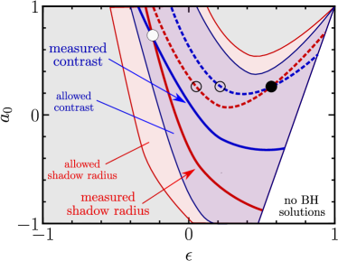
Figure 3: Schematic representation of the combined use of the shadow radius and of the intensity contrast to obtain constraints on the values of the coefficients of the RZ-metric. Shown respectively as shaded red and blue areas are the allowed regions for the RZ coefficients for the shadow radius and contrast, respectively. Indicated instead with solid lines are the constraints on the coefficients once a shadow radius (red line) and the contrast (blue line) have been measured with very high precision. Their intersection can then be used to set precise constraints on the coefficients (filled white circle). Note that the measurements of the shadow radius and contrast when considered alone can be degenerate (dashed red and blue lines), namely, multiple values of the coefficient $\epsilon$ can be used for the same value of the coefficient $a_{1}$ (empty circle). However, the intersection of the two measurements leads to a precise constraint of the coefficients (filled black circle). The panel refers to the RZ coefficients $a_{0}$ and $\epsilon$, but a similar logic can be applied when considering the coefficients $a_{1}$ and $\epsilon$. Figures 4 and 5 provide more quantitative examples of this schematic diagram.

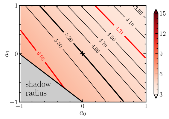
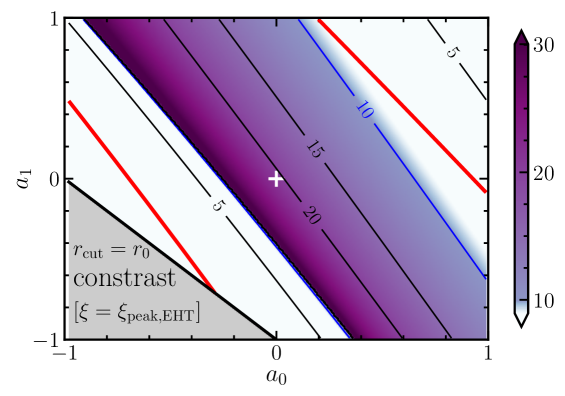
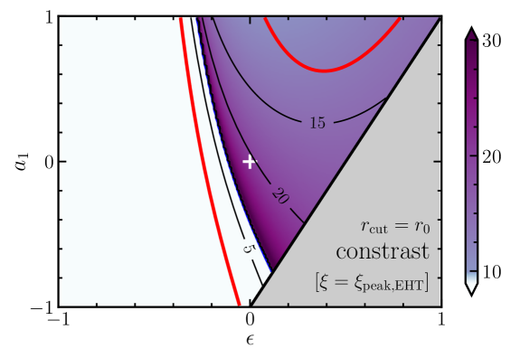
Figure 4: The variation in the shadow-size (top row), and the contrast in the BH image at $\xi=\xi_{{\text{peak, }}{\text{\tiny{EHT}}}}=5.5M$ (bottom row) for the principal two-parameter RZ BH models used here. The red lines in all plots show $\xi=3\sqrt{3}(1\pm 0.17)M$, the approximate $1\!-\!\sigma$ bounds of allowed shadow-sizes obtained by the EHT for M87^∗. When displaying the bottom row, we have allowed the emission region to extend all the way down to the event horizon (this row is the 2D analogue of the middle row of Fig. 2). Note that the peak in the contrast profile does not appear at $\xi=5.5M$, except for the BHs with shadow-sizes of $\xi_{\text{ps}}=5.5M$. Thus, if the emission is not suppressed close to the BH, the requirement that the peak-contrast in the image occur at $\xi=5.5M$ is an extremely stringent constraint, independent of the emission model. The gray region shows the “theoretically-disallowed” region of the relevant RZ parameter space (see Table 2). The crosses (black in the upper panels and white in the lower ones) locate the Schwarzschild BH and the dotted line represents the family of Reissner-Nordström (RN) BHs. The blue marker shows the $\bar{q}=0.9$ RN BH (see Kocherlakota et al. 2021).

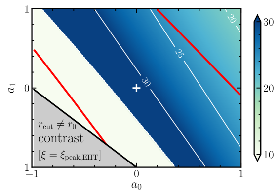
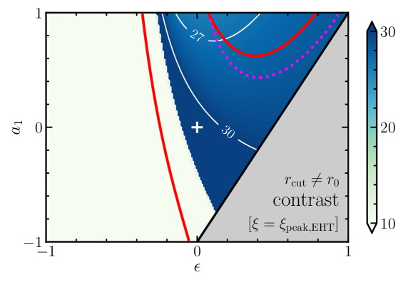
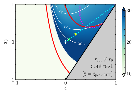
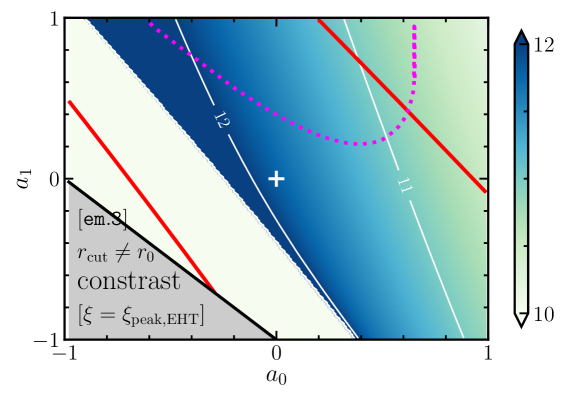
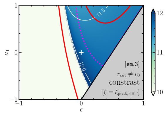
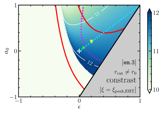
Figure 5: The variation in the contrast in the BH image at $\xi=\xi_{{\text{peak, }}{\text{\tiny{EHT}}}}=5.5M$ for the principal two-parameter RZ BH models used here. Here we impose an inner cut-off at $r_{\text{cut}}=r_{\text{tp}}(5.5M)$ so that one of the maxima in the contrast profile occurs at $\xi=5.5M$, i.e., at the “correct” location, with the other occurring as usual at the shadow boundary $\xi=\xi_{\text{ps}}$. Imposing such a cut-off is only possible for BHs with $\xi_{\text{ps}}>5.5M$ (i.e., not for the BHs in the light-green regions. The magenta lines show the region in which the global maximum occurs at $\xi=\xi_{\text{ps}}$ (corresponding to case B of Eq. 28). Therefore, in this region, the quantity shown here $\mathcal{C}(5.5M)$ only provides a lower bound for the peak contrast. The complementary region corresponds to the case when the peak occurs precisely at $\xi=5.5M$ (case C). From the top ($\mathtt{em.1}$) to the bottom row ($\mathtt{em.3}$) we have varied the emission coefficient prescription. The red lines denote, as usual, the EHT shadow-size bounds. The black cross locates the Schwarzschild BH and the cyan line represents the family of Reissner-Nordström (RN) BHs. The star and triangle markers locate the RN BHs with specific charges of $\bar{q}=0.50$ and $0.75$, respectively.

4 Variation of Observed Ring Size with Metric

In this section, we consider spherical accretion, as described in Sec. 2.1, onto Rezzolla-Zhidenko (RZ) BHs, and analyse the variation in the observed image properties with RZ parameters, which govern the deviation away from the Schwarzschild metric. Since we have already touched on the impact of modifying the emission model on the image properties, in Fig. 4, we will fix the emission prescription in this section to the one given in Eq. 17, and let the emission zone extend all the way down to the horizon ($r_{\text{cut}}=r_{0}$). In Fig. 5, we introduce an inner cutoff radius in the emission region such that a peak in the contrast profile occurs at the EHT-observed location, and also consider how varying the emission coefficient impacts our results.

As we will discuss below, it is sufficient for our present purposes to restrict our considerations here to the principal one-parameter and two-parameter subfamilies of the three-parameter family $\mathscr{M}(\epsilon;a_{0};a_{1})$ of RZ BHs, with $B^{2}=-g_{tt}g_{rr}=1$ and $a_{2}=0$, whose sole metric function can be written compactly as (Rezzolla & Zhidenko 2014; see also Konoplya et al. 2016 and Kocherlakota & Rezzolla 2020 for the extensions to axisymmetric BH spacetimes and to spherically-symmetric non-BH spacetimes respectively),

$$N^{2}(r)=1-\frac{2M}{r}+\frac{4a_{0}}{(1+\epsilon)^{2}}\frac{M^{2}}{r^{2}}+\frac{8(\epsilon-a_{0}+a_{1})}{(1+\epsilon)^{3}}\frac{M^{3}}{r^{3}}-\frac{16a_{1}}{(1+\epsilon)^{4}}\frac{M^{4}}{r^{4}}\,,$$ (20)

where $M$ is the ADM mass of the BH spacetime. As in Rezzolla & Zhidenko (2014), we will require that the outermost horizon (i.e., the largest zero of $g_{rr}^{-1}=N^{2}(r)=0$) be located at $r=r_{0}$, where

$$r_{0}:=\frac{2M}{1+\epsilon}\,.$$ (21)

Thus, $\epsilon>-1$ (alone) controls the size of the event horizon and $a_{0}$ measures the magnitude of violation of the solar system constraints ($|a_{0}|\lesssim 10^{-4}$; Will 2006). These constraints are not applicable to theories of gravity which do not admit a Birkhoff-like uniqueness theorem, thus supporting the study of metrics with $a_{0}\neq 0$. Furthermore, that no larger roots of $N^{2}=0$ should exist imposes non-trivial constraints on the 3D RZ parameter space. We tabulate these theoretical constraints for the principal axes and planes of this 3D space in Table 2.

The $tt$-metric function above can be compared to its asymptotic post-Newtonian (PN) expansion,

$$N^{2}=1-\frac{2M}{r}+2\sum_{n=1}^{\infty}\zeta_{n}\left(-\frac{M}{r}\right)^{n+1}\,,$$ (22)

where $\zeta_{1}$ is typically expressed as $\zeta_{1}:=\beta-\gamma$, with $\gamma$ the coefficient of the $\mathscr{O}(r^{-1})$-term in the asymptotic expansion of $g_{rr}$. In particular, for this family of BH metrics, the $tt$-PN expansion truncates at $\mathscr{O}(r^{-4})$, and it is possible to find a map between the two sets of parameters as,

$$\zeta_{1} =\ \frac{2a_{0}}{(1+\epsilon)^{2}}\,,$$ (23)

$$\zeta_{2} =\ -\frac{4(\epsilon-a_{0}+a_{1})}{(1+\epsilon)^{3}}\,,$$ (24)

$$\zeta_{3} =\ -\frac{8a_{1}}{(1+\epsilon)^{4}}\,.$$ (25)

We indicate which PN parameters vanish for the various sections of the $\mathscr{M}(\epsilon;a_{0};a_{1})$ family we consider here in Table 2.

We also explicitly report the Ricci and Kretschmann curvature scalars, $\mathscr{R}$ and $\mathscr{K}$, for these RZ BHs to show that these spacetimes are regular everywhere except at the central singularity $r=0$,

$$\mathscr{R}= \ 4M^{3}r^{-6}(\zeta_{2}r-3M\zeta_{3})$$ (26)

$$\mathscr{K}= \ 16M^{2}r^{-12}\left[3r^{6}-12M\zeta_{1}r^{5}+2M^{2}(7\zeta_{1}^{2}+10\zeta_{2})r^{4}\right.$$

$$\ \left.-10M^{3}(5\zeta_{1}\zeta_{2}+3\zeta_{3})r^{3}+2M^{4}(39\zeta_{1}\zeta_{3}+23\zeta_{2}^{2})r^{2}\right.$$

$$\ \left.-146M^{5}\zeta_{2}\zeta_{3}r+117M^{6}\zeta_{3}^{2}\right]$$ (27)

Considering the particular case of the $\mathscr{M}(\epsilon)-$RZ family, it is easy to see that there is a bijective map between the metric functions with $1/2\leq\epsilon<\infty$ and those with $-1<\epsilon\leq 1/2$: the only metric-deviation parameter $\zeta_{2}(\epsilon)$ is double-valued on $-1<\epsilon<\infty$. Therefore, by setting the “theoretical priors,” $-1<\epsilon\leq 1/2$, we consider (a) all unique $\mathscr{M}(\epsilon)-$RZ BH solutions while ensuring also that (b) $r_{0}(\epsilon)=2M/(1+\epsilon)$ locates the event horizon. For $\epsilon>1/2$, $r_{0}(\epsilon)$ corresponds to the inner horizon with $r=\left(\epsilon+\sqrt{4\epsilon+\epsilon^{2}}\right)/(1+\epsilon)$ then locating the outer event horizon. In other words, within the ranges in which the RZ parameters are here chosen, the metric does not show any pathology.

Table 2 demonstrates how the theoretically-allowed range of a given parameter that characterises a particular structural deviation in the spacetime metric from Schwarzschild depends on the overall form of the metric itself. Notice, e.g., the striking case of the $\epsilon$ parameter: its theoretically-allowed domain changes character from being bounded when only $\epsilon$ is allowed to vary, to being unbounded otherwise. Thus, as a corollary, constraints from experiment on any given parameter (RZ or PN) will, in general, depend on the full form of the metric in use (see also Völkel & Barausse 2020). We demonstrate this below explicitly by considering both one-parameter and two-parameter subfamilies of the RZ metric. This does not a priori rule out the existence of an observation-specific set of parameters or a combination thereof on which “robust” (independent of the overall form of the metric; even if only as a good approximation) constraints may be set. In the absence of knowledge of such a combination, it can be useful to report constraints on the single-parameter RZ BH metrics, as done e.g. in The Ligo Scientific Collaboration et al. (2021), where the PN formalism was used instead. Also, since we will report our findings entirely in terms of RZ parameters, we note that the non-linear map between the two sets of coefficients implies translating observational constraints from the RZ- to the PN-space can yield drastically differing inferences, especially when $\epsilon\gtrsim-1$.

We further limit the range of our demonstrative exploration of images of RZ BHs to the region of “small” parametric deviations, $\Delta<1$, where $\Delta:=\max{\left(|\epsilon|,|a_{0}|,|a_{1}|\right)}$ is the infinity norm on the space and measures the magnitude of the parametric deviation of an RZ BH from the Schwarzschild spacetime (Kocherlakota & Rezzolla, 2020). This allows us to focus on BH spacetimes that are relatively similar to the Schwarzschild spacetime since, e.g., we find that there exist parameter regions for $\Delta>1$ for which the (quartic) CNG equation (14) admits multiple roots $r>r_{0}$ (cf. Gan et al. 2021). We relegate a systematic exploration of these regions to future work.

In addition to the EHT measurements of $\xi_{{\text{peak, }}{\text{\tiny{EHT}}}}$ and $C_{\text{peak, EHT-min}}$ that we have used above, since changes in the spacetime metric can cause changes in the observed size of the shadow, we will also compare how the EHT inference of the shadow-size of M87^∗, $3\sqrt{3}(1-0.17)M\lesssim r_{\text{sh}}:=\xi_{\text{ps}}\lesssim 3\sqrt{3}(1+0.17)M$ (Event Horizon Telescope Collaboration et al., 2019f; Kocherlakota et al., 2021), constrains the RZ parameter space. We also comment on the consistency between these two sets of bounds when using non-Kerr BHs, whilst remaining within the modest ambit of the toy accretion-emission models in use here.

We show the variation in the sizes of the horizon, photon sphere, and shadow for the single-parameter models in the top row of Fig. 2. For small-deviations from the Schwarzschild spacetime, the variation in the shadow radius $\xi_{\text{ps}}$ is approximately linear with respect to the relevant metric parameter for the $\mathscr{M}(a_{0})$ and $\mathscr{M}(a_{1})$ BH models, i.e., when the horizon size is held fixed to its Schwarzschild value. The variation in the photon sphere size is also approximately linear with respect to $a_{1}$ for $\mathscr{M}(a_{1})$ BHs since $a_{1}$ modifies the metric at a higher order in $r^{-1}$. The horizontal white bands indicate the allowed range of these parameters, for the single-parameter metrics, as inferred from the shadow-size bounds discussed above. We show the corresponding contrast profiles for these single-parameter BH metrics in the second row, when the emission region extends all the way down to the horizon. As in Fig. 1, we show $\xi_{{\text{peak, }}{\text{\tiny{EHT}}}}$ and $\mathcal{C}_{\text{peak, EHT-min}}$ as vertical orange and horizontal cyan lines respectively. It is clear then that BHs that have shadow-sizes $\xi_{\text{ps}}\gnsim 5.5M$ would in general appear to have bright rings larger than the one measured by the EHT, $\xi_{\text{peak}}\gnsim\xi_{{\text{peak, }}{\text{\tiny{EHT}}}}$. On the other hand, BHs with smaller shadow-sizes could satisfy $\xi_{\text{peak}}=\xi_{{\text{peak, }}{\text{\tiny{EHT}}}}$ if the emission regions in their spacetimes did not extend all the way down to the horizon but were instead cut-off at some radius outside their respective photon spheres for some reason. In this case however, as we have seen above in Sec. 3, the maximum contrast in the image of such BH would be reduced, from infinity to some finite value, when $r_{\text{cut}}>r_{\text{ps}}$. To this end, we consider RZ BHs with $\xi<\xi_{{\text{peak, }}{\text{\tiny{EHT}}}}$ and show the contrast profiles when $r_{\text{cut}}=r_{\text{tp}}(\xi_{{\text{peak, }}{\text{\tiny{EHT}}}})$ in the bottom row of Fig. 2. We see that since the leading-order change in the $tt$-metric function introduced by the $\epsilon$ or the $a_{1}$ parameter is at $\mathscr{O}(r^{-3})$, the impact of small-variations ($\Delta<1$) in these parameters on the value of the peak contrast is relatively smaller than in the case of small-variations in the $\mathscr{M}(a_{0})$ model, where the metric is modified already at $\mathscr{O}(r^{-2})$. We also show the impact of varying the emission model, and demonstrate that it should be possible to constrain the “astrophysics,” i.e., the exponent of the emission coefficient, and/or the spacetime metric, with the help of additional observables such as the maximum contrast in the image. Thus, bounds on the RZ parameter from both sides are to be generically anticipated. Finally, we note that if the shadow-size of a BH is “sufficiently smaller” than the EHT-observed location of the contrast peak, i.e., $\xi_{\text{ps}}\ll\xi_{\text{peak-EHT}}$ and/or the emission coefficient is “sufficiently soft”, (i.e., decaying more slowly with distance) , then the location of the absolute maximum in the contrast profile shifts back from $\xi=\xi_{\text{tp}}(r_{\text{cut}})$ to the shadow boundary $\xi=\xi_{\text{ps}}$. We discuss these aspects in more detail in Sec. 5. This indicates that the two-sided bounds discussed above will generically exist even when the restriction on the size of the deviations $\Delta<1$ imposed here is lifted.

We shift our focus now to the question of whether multi-parameter parametrized metrics can also be meaningfully constrained when using the same set of observables. For our present demonstrative purposes, we use here the two-parameter RZ models to explore the change in the bounds inferred on the individual parameters when changing the overall structure of the metric. First, with a cartoon, we visualise the impact, on the parameter space of the $\mathscr{M}(\epsilon,a_{0})$ RZ BHs, of the EHT shadow-size constraints (red bands) and the reported minimum bound of the peak-contrast in the image (blue bands) in Fig. 3. The red lines (solid and dashed) represent shadow-size isocontours whereas the blue lines show two sample peak-contrast isocontours, when the peak occurs at $\xi=5.5M$. If in the future we are able to constrain the shadow-sizes of supermassive compact objects such as M87^∗ or Sgr A^∗ with increasing precision, the width of the red band would shrink and thus constrain the RZ parameter space more severely. A similar statement holds for the blue band if the flux-sensitivity of the EHT can be increased. As will become evident from the figures below, while these bands overlap significantly, these constraints are not in general degenerate. In the limit of infinite precision, picking out a single shadow radius yields at best a family of two-parameter RZ BHs (solid- or dashed-red lines in this figure), while a precise peak contrast measurement would pick out a different family of RZ BHs (solid- or dashed-blue lines) in general. Thus, with two observables, it should be possible to uniquely determine the underlying metric parameters of a 2D family of BHs. Interestingly, as can be seen from this figure, it is possible for two BHs with differing horizon sizes to have identical shadow-sizes (filled circle and empty circle, both lying on the same red-line).

More concretely, the variation in the shadow-sizes, as well in the value of the contrast in the image at $\xi=\xi_{{\text{peak, }}{\text{\tiny{EHT}}}}$, when the emission zone extends all the way to the horizon, with the relevant RZ parameters for the 2D RZ BHs is reported in Fig. 4. The red lines in all figures bound the region in which the EHT shadow-size bounds are respected. As above, the (blue) contours $\mathcal{C}(\xi=\xi_{{\text{peak, }}{\text{\tiny{EHT}}}})=10$ in Fig. 4 represent the bounds obtained from the requirement that $\mathcal{C}(\xi_{{\text{peak, }}{\text{\tiny{EHT}}}})>\mathcal{C}_{\text{peak, EHT-min}}$. Thus, the first takeaway is that BHs with shadow-sizes larger than $\xi_{{\text{peak, }}{\text{\tiny{EHT}}}}$ fail to meet the contrast constraint, whereas those that have significantly smaller shadow-sizes are also expected to fail, for the reasons discussed above. Notice however that since we do not cut off the emission outside the horizon, the peak in the contrast profile must necessarily occur at $\xi=\xi_{\text{ps}}$. Therefore, if $\xi_{\text{ps}}\neq\xi_{{\text{peak, }}{\text{\tiny{EHT}}}}$, the contrast peak in the image does not occur at the EHT-observed location.

Furthermore, the observed lower bound on the peak contrast imposes no additional constraints on the RZ parameter space in this scenario ($r_{\text{cut}}=r_{0}$), and no insight into the emission coefficient is possible (see Sec. 5). $\alpha$, which we have used to locate the observed peak in the contrast, is of finite precision (limited in part by the angular resolution of the EHT array in 2017), we expect a small spread in this “allowed” region around $\xi_{\text{ps}}=\xi_{{\text{peak, }}{\text{\tiny{EHT}}}}$. The consistency of the two bands of constraints – location of the contrast-peak and shadow-size – demonstrates a null-test of the calibration procedure employed by the EHT to obtain the latter from the former. While the test here is limited due to the restriction to spherical symmetry and a fixed BH ADM mass, our approach involving analytical models is very efficient as a path-finding step for further exploration of the parameter space with numerical simulations. We explore the impact of using the observed ring width, another useful observable that is sensitive to the gradient of the emission coefficient, in the following section for single-parameter BH models.

Finally, we note that the EHT-allowed range of a particular parameter depends on the underlying metric. We see that while for the $\mathscr{M}(\epsilon)$ BH models, we find $-0.22\lesssim\epsilon\leq 0.5$ to be the EHT-allowed range, it is immediately evident from Fig. 4, that the allowed range for $\epsilon$ is quite significantly different for the $\mathscr{M}(\epsilon;a_{1})$ and $\mathscr{M}(\epsilon;a_{0})$ models.

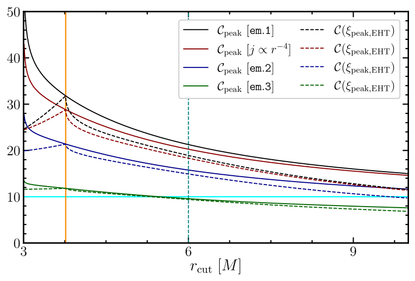
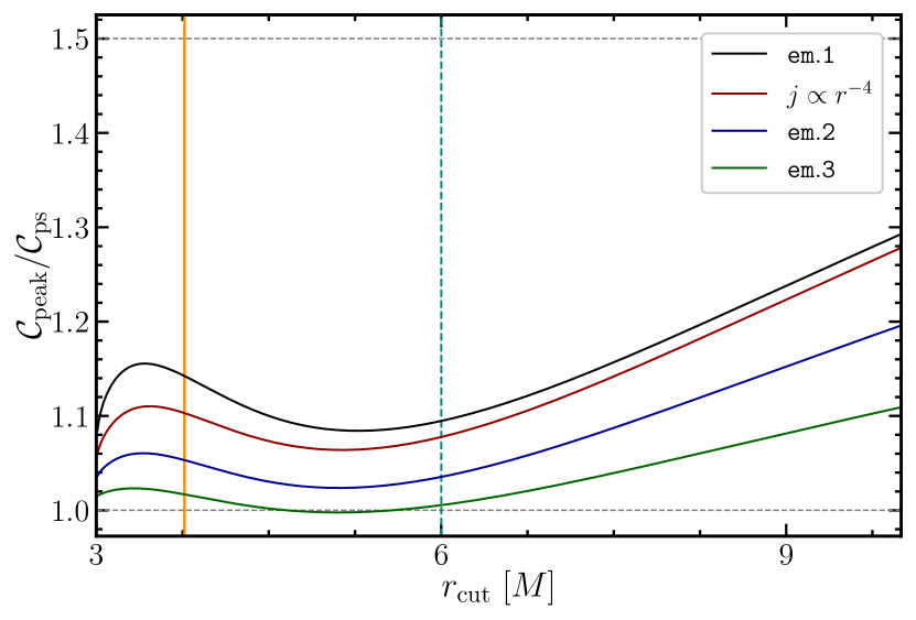
Figure 6: In the left panel, we show the variation in the peak value of the contrast in the image of a Schwarzschild BH with varying $r_{\text{cut}}$. In the right panel, the relative difference in the peak contrast and the contrast at the shadow boundary is displayed. The vertical orange and green lines correspond to $r=r_{\text{tp}}(\xi_{{\text{peak, }}{\text{\tiny{EHT}}}})\approx 3.77M$ and $r=6M$, respectively.

We show in Fig. 5 the contrast at $\xi_{{\text{peak, }}{\text{\tiny{EHT}}}}$ when one of the contrast maxima also occurs at this location, i.e., for $r_{\text{cut}}=r_{\text{tp}}(\xi_{{\text{peak, }}{\text{\tiny{EHT}}}})$. To explore the impact of varying the emission prescription, we show in the top and bottom rows the two emission models $\mathtt{em.1}$ and $\mathtt{em.3}$ respectively. As expected, on introducing this cutoff, for BHs with $\xi_{\text{ps}}<\xi_{{\text{peak, }}{\text{\tiny{EHT}}}}$, the value of the contrast at $\xi_{{\text{peak, }}{\text{\tiny{EHT}}}}$ increases (compare the bottom row of Fig. 4 with the top row of Fig. 5), thus making weak the bounds imposed by the lower bound of the peak-contrast obtained by the EHT. At the same time, unsurprisingly, for the “softer” (fall-off) emission prescription, we find tighter constraints on the RZ parameter space from the lower bound on the peak-contrast. Thus, even in the most conservative case ($\mathtt{em.1}$), while the contrast-constraints do not appear in the $\Delta<1$ region of the parameter space, it is evident that with increasingly better observations, metric tests will only get better and increasingly more robust.

The figure also hints at the possibility that there exist regions of total degeneracy, where two-parameter families of BHs may have the same shadow-size and approximately the same $\mathcal{C}(\xi_{{\text{peak, }}{\text{\tiny{EHT}}}})$ values (and possibly the same contrast profiles), e.g., in the top right regions in the $\epsilon\!-\!a_{0}$ and $\epsilon\!-\!a_{1}$ parameter spaces. This degeneracy could in principle be broken by introducing new observables such as the fractional-width of the ring in the observed image (see the discussion in Sec. 5) or the locations of the photon sub-ring and the Lyapunov exponent, the latter of which we explore in upcoming work (Kocherlakota et al., 2022).

5 Fractional Width of the Observed Ring as a Discriminator of Emission Model

In this section we consider the definition of the width of the observed circular ring, and explore its use in obtaining insights into local emission physics.

For a Schwarzschild BH, we show in the left panel of Fig. 6 the variation in the peak contrast with changing emission region cut-off location $r_{\text{cut}}$. This figure demonstrates that independently of the emission model, requiring a large cut-off radius, to push the peak in the observed image to larger sizes in order to match the EHT reported value of $\xi_{{\text{peak, }}{\text{\tiny{EHT}}}}=5.5M$ can be effective. However, for significantly larger $r_{\text{cut}}$, the peak-contrast value falls below the EHT reported value of $\mathcal{C}_{\text{peak, EHT-min}}=10$. In the right panel, we show the fractional difference between the peak contrast and the contrast at the photon sphere for different $r_{\text{cut}}$, to measure the drop in the contrast from the observed peak to the shadow boundary. We note in particular that $\mathcal{C}_{\text{ps}}>0.5\mathcal{C}_{\text{peak}}$, at least for $3<r_{\text{cut}}/M<9$. Thus, a truly sharp drop in the contrast occurs always close to the shadow boundary, $\xi=\xi_{\text{ps}}$. The non-monotonic behaviour of the curves shown here appears to stem from the non-monotonic behaviour of the redshift function for photons emitted radially-inwards, $\gamma_{-}$ (see the left panel of Fig. 11).

We denote by $w$ the width of the observed ring defined, within the context of the spherical models we use here, using the “half-peak” location(s), $\xi^{\pm}_{\text{hp}}:=\xi^{\pm}(\mathcal{C}_{\text{peak}}/2)$, where the contrast becomes half of the peak contrast value, with the superscripts $\pm$ denoting that $\xi^{+}_{\text{hp}}>\xi_{\text{peak}}$ and vice-versa. For the case when $r_{\text{cut}}=r_{0}$, since the peak contrast value necessarily occurs at the shadow boundary and is mathematically infinite, $\mathcal{C}_{\text{ps}}:=\mathcal{C}(\xi=\xi_{\text{ps}})\rightarrow\infty$, we use $w=0$. When $\xi_{\text{ps}}<\xi_{{\text{peak, }}{\text{\tiny{EHT}}}}$, introducing an ad hoc interior cut-off radius for the emission region becomes possible. As discussed above, the only way to find the location of the bright emission-ring to correspond to the one measured in the M87* image in the present set up is to set $r_{\text{cut}}=r_{\text{tp}}(\xi_{{\text{peak, }}{\text{\tiny{EHT}}}})$. The contrast values of the two (finite) maxima in this case, i.e., $\mathcal{C}_{\text{ps}}$ and $\mathcal{C}_{{\text{peak, }}{\text{\tiny{EHT}}}}:=\mathcal{C}(\xi_{{\text{peak, }}{\text{\tiny{EHT}}}})$, outline four possibilities

$$w=\left\{\begin{aligned} &\xi^{+}_{\text{hp}}-\xi_{\text{ps}}\,,\ \ &&\mathcal{C}_{\text{ps}}>2\mathcal{C}_{{\text{peak, }}{\text{\tiny{EHT}}}}&&\quad\quad{\rm[case\ A]}\\ &\xi^{+}_{\text{hp}}-\xi_{\text{ps}}\,,\ \ &&2\mathcal{C}_{{\text{peak, }}{\text{\tiny{EHT}}}}\geq\mathcal{C}_{\text{ps}}>\mathcal{C}_{{\text{peak, }}{\text{\tiny{EHT}}}}&&\quad\quad{\rm[case\ B]}\\ &\xi^{+}_{\text{hp}}-\xi_{\text{ps}}\,,\ \ &&\mathcal{C}_{{\text{peak, }}{\text{\tiny{EHT}}}}\geq\mathcal{C}_{\text{ps}}\geq\mathcal{C}_{{\text{peak, }}{\text{\tiny{EHT}}}}/2&&\quad\quad{\rm[case\ C]}\\ &\xi^{+}_{\text{hp}}-\xi^{-}_{\text{hp}}\,,\ \ &&\mathcal{C}_{{\text{peak, }}{\text{\tiny{EHT}}}}/2>\mathcal{C}_{\text{ps}}&&\quad\quad{\rm[case\ D]}\,,\end{aligned}\right.$$ (28)

with $\xi_{\text{peak}}=\xi_{\text{ps}}$ in cases A and B and $\xi_{\text{peak}}=\xi_{{\text{peak, }}{\text{\tiny{EHT}}}}$ otherwise.

In the first two cases, the global maximum of the contrast profile occurs at the shadow boundary even when an inner cut-off radius for the emission is invoked. However, in these cases, the width of the ring $w$ is clearly non-zero. Furthermore, in case A, $\xi=\xi_{{\text{peak, }}{\text{\tiny{EHT}}}}$ lies outside the ring width. In case C, the peak of emission occurs at $\xi=\xi_{{\text{peak, }}{\text{\tiny{EHT}}}}$ with the shadow boundary forming the inner edge of the emission-ring. Finally, case D represents a scenario where the emission ring would appear to be disjoint from the shadow boundary. For all of the metric deviations and all of the emission models we consider here, we find that cases A and D are never realised. We direct the reader to see Fig. 5 where the only scenarios that appear to be possible, when $\xi_{\text{ps}}<\xi_{{\text{peak, }}{\text{\tiny{EHT}}}}$ and $r_{\text{cut}}=r_{\text{tp}}(\xi_{{\text{peak, }}{\text{\tiny{EHT}}}})$, are case B (demarcated by the blue lines) and case C. Thus, the inner edge of the observed emission ring is always bounded by the shadow boundary independently of whether or not there is an inner cut-off to the region of emission. This is a central result of the current work which has recently been subject to debate (see, e.g., Gralla 2021).

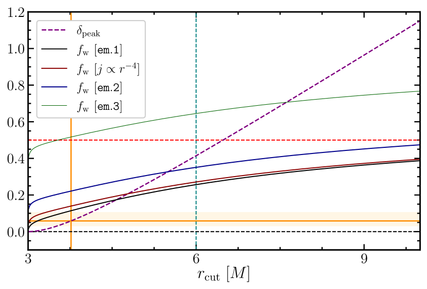
Figure 7: We show here the variation, for the Schwarzschild BH, in the location of the peak in the contrast profile relative to the shadow-size, $\delta_{\text{peak}}:=\xi_{\text{peak}}/\xi_{\text{ps}}-1$, when the emission region has an artificial interior cutoff at $r=r_{\text{cut}}$. We also display the change in the fractional-width of the observed ring in the image, $f_{\text{w}}:=w/2\xi_{\text{peak}}$ with $r_{\text{cut}}$. The fractional-width of the ring could be a useful observable to restrict the emission coefficient $j$. The vertical orange and green lines have the same meaning as in Fig. 6. The dashed-red line shows the EHT bound, $f_{\text{w}}\leq 0.5$.

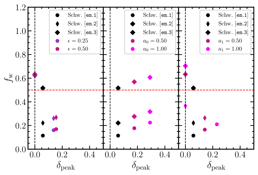
Figure 8: We show here the variation, for the single-parameter RZ BHs, in $\delta_{\text{peak}}$ and $f_{\text{w}}$ with the relevant deviation parameter, for $r_{\text{cut}}=r_{\text{tp}}(\xi_{{\text{peak, }}{\text{\tiny{EHT}}}})$. We see that the soft emission prescription $j=k_{2}r^{-2}~{}[\mathtt{em.3}]$ typically fails the $f_{\text{w}}\lesssim 0.5$ bound [dashed-red line], demonstrating how this observable can be used to constrain emission physics. The clear correlation with the metric deviation parameter also indicates how tests of gravity may be possible with this observable. See also the bottom row of Fig. 2

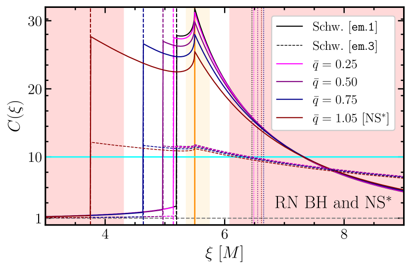
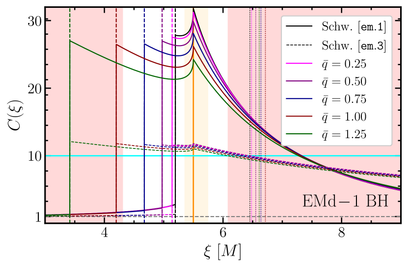
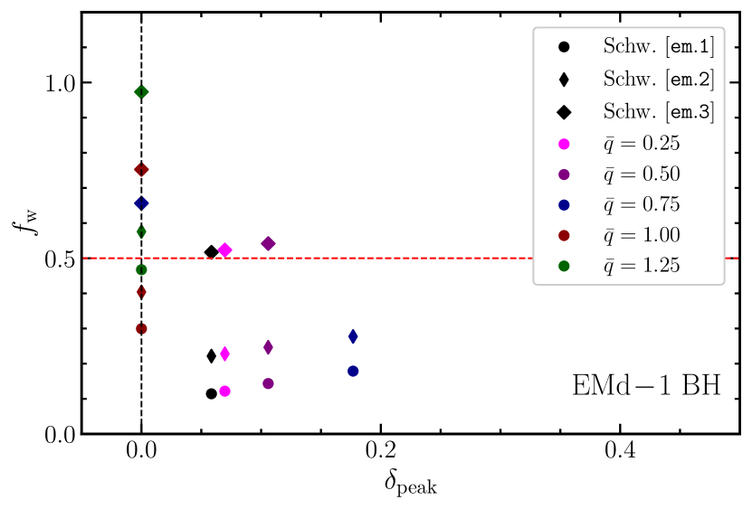
Figure 9: In the left panels, we display the variation in the observed contrast $\mathcal{C}$ for a series of Reissner-Nordström (RN) and Einstein-Maxwell-dilaton-1 (EMd-1) BHs, with increasing specific charges, $\bar{q}=q/M$. We also discuss the case of a single RN naked singularity (NS^∗) The vertical dashed correspond to the size of the shadow cast by the compact object, whereas the vertical dotted lines denote the half-peak location for the emission model $[\mathtt{em.1}]$. The remaining lines and shaded-regions retain their meaning from Fig. 6 and Fig. 2. In the right panels, we show the corresponding fractional deviation of the contrast peak relative to the shadow-size $\delta_{\text{peak}}$ and the fractional width of the ring relative to the shadow diameter $f_{\text{w}}$ (compare with left panels). This figure demonstrates how the maximum observed contrast in the image is sensitive to $j$, whereas the width of the ring can potentially be used to test gravity. The dashed-red line shows the EHT reported bound, $f_{\text{w}}\leq 0.5$, for comparison.

In Fig. 7, for the Schwarzschild BH, we show the fractional-deviation of the location of the observed peak from the shadow boundary $\delta_{\text{peak}}:=\xi_{\text{peak}}/\xi_{\text{ps}}-1$ and the fractional-width of the observed ring relative to the observed ring diameter $f_{\text{w}}:=w/2\xi_{\text{peak}}$ (see, e.g., Sec. 7.2 of Event Horizon Telescope Collaboration et al. 2019f). The EHT reports a maximum value of $f_{\text{w}}\lesssim 0.5$. It is interesting to note that the range of $r_{\text{cut}}$ for which the observed contrast peak appears at the location seen by the EHT also satisfies the fractional-width constraint, despite the underlying accretion-emission model being highly simplistic, only for sufficiently steep (large-$n$) emission coefficients. Thus, the fractional-width of the ring can be yet another promising discriminator of emission physics.

In Fig. 8, we show the variation of $\delta_{\text{peak}}$ and $f_{\text{w}}$ for the various one-parameter RZ BH models, with varying emission coefficient and spacetime metric. Here we use $r_{\text{cut}}=r_{\text{tp}}(\xi_{{\text{peak, }}{\text{\tiny{EHT}}}})$ to force the peak in the observed contrast to appear at the EHT observed location, $\xi=\xi_{{\text{peak, }}{\text{\tiny{EHT}}}}$. It becomes clear from this figure that this is not always possible for BHs with sufficiently small shadow sizes, $\xi_{\text{ps}}\ll\xi_{{\text{peak, }}{\text{\tiny{EHT}}}}$. Note how either a soft emission coefficient or a small shadow-size can cause the peak at $\xi=\xi_{{\text{peak, }}{\text{\tiny{EHT}}}}$ to become a secondary local maximum.

Finally, to ascertain which features and possibilities discussed here can appear when using BH and non-BH spacetimes that arise as solutions in various known theories of gravity, we consider the image properties of the Reissner-Nordström (RN) BHs and of the Gibbons-Maeda-Garfinkle-Strominger-Horowitz (Gibbons & Maeda, 1988; Garfinkle et al., 1991), which we shall refer to as the EMd-1 BHs. These BHs arise as static, charged solutions of the Einstein-Maxwell equations and of the Einstein-Maxwell-dilaton low-energy effective action of the heterotic string respectively. We also consider a RN naked singularity (NS^∗) spacetime for completeness. In Fig. 9 we show the contrast profiles of the RN and EMd-1 BHs such that a maximum occurs at the EHT observed value $\xi=\xi_{{\text{peak, }}{\text{\tiny{EHT}}}}$. Notice however that since the shadow-size decreases monotonically with specific charge in both cases, for sufficiently small shadow-sizes the peak at $\xi=\xi_{{\text{peak, }}{\text{\tiny{EHT}}}}$ is only a secondary local maximum. Thus, such BH solutions would be ruled out, at least within the accretion and emission models we use here. Finally, we note also that the RN BH is exactly described by the $\mathscr{M}(\epsilon,a_{0})$ RZ BH metric with $\epsilon(\bar{q})=a_{0}(\bar{q})=2/(1+\sqrt{1-\bar{q}^{2}})-1$, where $\bar{q}=q/M$ is the specific electromagnetic charge of the BH (see, e.g., Kocherlakota & Rezzolla, 2020). We mark with a red dotted line this family of BHs in the $(\epsilon,a_{0})$ parameter space in Figs. 4 and 5 for ready comparison.

As can be seen from this figures in this section the fractional-width of the ring always increases when the emission model becomes softer (i.e., smaller-$n$ for $j=k_{n}r^{-n}$), as anticipated. We expect that when using more realistic accretion and emission models, this observable will continue to remain an excellent observable with which the EHT can constrain both emission physics and spacetime geometry.

6 Conclusions and Discussion

We have studied here radially freely falling accretion onto spherically-symmetric BHs, whose spacetime geometries are characterized in general by three-parameters $\{\epsilon,a_{0},a_{1}\}$. To study features of the image formed on the observer’s sky we employ various isotropic, monochromatic emission models that are characterized roughly by the radial profile of the emission coefficient $j\sim r^{-n}$. Further, to study the impact of artificially suppressed emission close to the event horizon, we introduce the parameter $r_{\text{cut}}$, the radius inside which we set $j=0$.

For this set of accretion-emission models, we find that the observed size of the bright ring, characterized by the location of the peak of the intensity contrast $\xi=\xi_{\text{peak}}$, is independent of the emission coefficient $j$. However, $\xi_{\text{peak}}$ increases monotonically with $r_{\text{cut}}$. Since it is possible to push out the location of the peak in the contrast profile by modulating $r_{\text{cut}}$, for BHs with shadow-sizes smaller than the observed size of the peak of emission in the EHT image of M87^∗, $\xi_{\text{ps}}<\xi_{{\text{peak, }}{\text{\tiny{EHT}}}}$, one can find a cutoff radius, $r_{\text{cut}}=r_{\text{tp}}(\xi_{{\text{peak, }}{\text{\tiny{EHT}}}})$, such that the contrast peak occurs exactly at the EHT observed location. BHs with shadow-sizes larger than $\xi_{{\text{peak, }}{\text{\tiny{EHT}}}}$ are ruled out since the location of the peak contrast in their images can never occur at $\xi=\xi_{{\text{peak, }}{\text{\tiny{EHT}}}}$. It is also possible in principle to constrain BHs with very small shadow-sizes when they violate the condition $\mathcal{C}_{\text{peak}}=\mathcal{C}(\xi_{{\text{peak, }}{\text{\tiny{EHT}}}})>\mathcal{C}_{\text{peak, EHT-min}}$. Additionally, for BHs with very small shadow-sizes ($\xi_{\text{ps}}\ll\xi_{{\text{peak, }}{\text{\tiny{EHT}}}}$), the contrast peak shifts back to the shadow boundary, with $\xi=\xi_{{\text{peak, }}{\text{\tiny{EHT}}}}$ locating only a secondary local maximum, when $r_{\text{cut}}=r_{\text{tp}}(\xi_{{\text{peak, }}{\text{\tiny{EHT}}}})$. Thus, using the measurement of the location of the peak contrast along with its measured lower bound imposes constraints on the space of metric-deviation parameters. Note that since the emission coefficient is primarily responsible in setting the scale of the contrast in the image, and “softer” emission coefficients (small-$n$) imply tighter constraints, it is indeed possible to set conservative bounds using the emission model we have proposed here [$\mathtt{em.1}$; see Sec. 2.3]; this model accounts for the entire binding energy of cold infalling fluid. Finally, we can also use simultaneously the shadow-size bounds reported by the EHT to constrain further the RZ parameter spaces. While the “constraint bands” we report from these two sets of measurements (location and value of the image contrast peak on the one side and the shadow bounds on the other) show overlap, as they should, they are typically not degenerate, as evidenced by the shape of the contour lines.

There is no a priori reason for emission to cease at some inner radius outside the event horizon $r_{\text{cut}}>r_{0}$ at least within the present context of spherical accretion. Thus, if we set $r_{\text{cut}}=r_{0}$ and consider the various two-parameter family of RZ BHs, we then find that the constraints on the relevant parameter spaces that we obtain by imposing the requirement that the location of the peak in the observed contrast profile coincide with the EHT-reported value, $\xi_{\text{peak}}=\xi_{{\text{peak, }}{\text{\tiny{EHT}}}}=\alpha M/2\approx 5.5M$, are far more severe than the EHT shadow-size bounds. Essentially, the former imposes the condition that $\xi_{\text{ps}}\approx 5.5M$, and is equivalent to an extremely precise shadow-size measurement. Even in this case, for higher-dimensional BH parameter spaces, it is not impossible to constrain exactly the spacetime metric of M87^∗. To break these types of inevitable degeneracies, we require additional observables, such as the fractional size of the ring width $f_{\text{w}}$ that the EHT has measured (Event Horizon Telescope Collaboration et al. 2019a; see, e.g., Fig. 7) or the sizes of photon subrings that the ngEHT hopes to observe soon. At the same time, it is also clear that the constraints we are able to establish on general properties of the spacetime near M87^∗, such as the size of the photon sphere or the event horizon ($\epsilon$), using presently available EHT measurements are nevertheless substantial. This is particularly relevant for various well-known solutions of alternative theories of gravity, where the arbitrary multi-pole moments of the BH metric are controlled by a small number of parameters or “charges” (see, e.g., Kocherlakota et al. 2021 and compare with Kocherlakota & Rezzolla 2020).

A significant limitation of the present work involves our use of a spherical accretion model, which implies that the redshifts and effective path-lengths shown in Sec. 2.1 may be modified significantly when working, e.g., even with emission sourced from stationary geometrically-thick tori. While in the latter case naturally the circular symmetry of the image on the celestial plane is lost, more importantly, the sharp drop in contrast at the shadow boundary may change due effectively to reduced Doppler beaming. At the same time, we do not expect significant qualitative changes in the results we have discussed above, with the advantage that these have been obtained without the use of GRMHD or ray-tracing codes: when using about $10^{4}$ grid points (BH metrics) to generate the contrast contour plots shown in Figs. 4 and 5, our code runs for less than a day on a standard laptop. In the same spirit, it would be useful to characterize in future the percentage changes in the various image-domain features we have explored here when employing more realistic semi-analytic accretion-emission models as well as ray-traced images of GRMHD simulations involving hot, magnetized accretion flows around Rezzolla-Zhidenko BHs.

While this work was in preparation, some of these issues have recently been addressed in Bauer et al. (2021), where the $\mathscr{M}(a_{1})-$RZ metric is also used, as well as in Ozel et al. (2021) and Younsi et al. (2021), where analytic models away from spherical symmetry are considered. In particular, it is worth noting that the range of the single-parameter $|a_{1}|<0.2$ adopted by Bauer et al. (2021) is considerably smaller than what is investigated here (see Table 2), leading to a suppression of the variation of the characteristic size of the emission ring around an RZ black hole with spacetime geometry (see Fig. 8). This is highly restrictive since the bounds on the parameter $a_{1}$ that one can infer from the shadow-size measurement of M87^∗ (see the top right panel of Fig. 2) are approximately an order-of-magnitude larger. Our results are also in agreement with those in Sec. 2 of Ozel et al. (2021), where spherical accretion is also considered. While Ozel et al. (2021) and Younsi et al. (2021) argue that the size of the bright emission ring is not disjoint from the shadow boundary using semi-analytic non-spherical accretion and emission models around Kerr and non-Kerr black holes respectively, we establish the same here by introducing an agnostic inner cut-off for the emission region, albeit within spherical symmetry, which has been a point of recent debate (see, e.g., Gralla 2021).

Acknowledgements: It is a pleasure to thank Ramesh Narayan for insightful discussions on emission coefficients, and Enrico Barausse, Guillermo Delgado, and Sebastian Voelkel for comments. We also thank our EHT colleagues for useful suggestions. Support comes from the ERC Synergy Grant “BlackHoleCam: Imaging the Event Horizon of black holes” (Grant No. 610058) and from the ERC Advanced Grant “JETSET: Launching, propagation and emission of relativistic jets from binary mergers and across mass scales” (Grant No. 884631).

Appendix A Schwarzschild Black Hole: Photon Radial Motion and Redshift

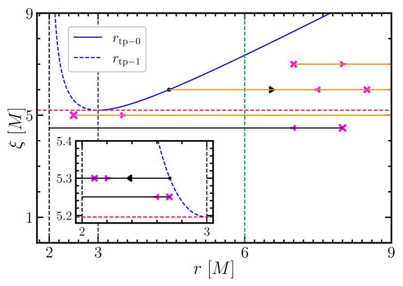
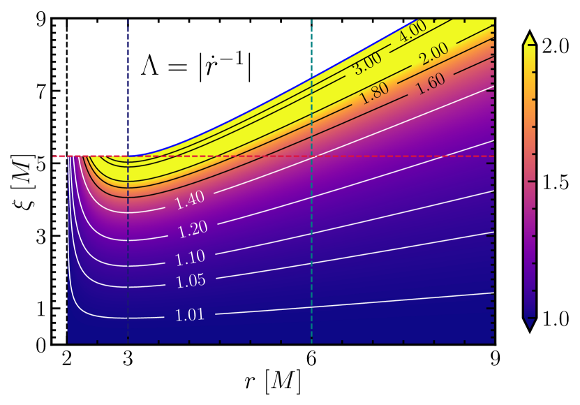
Figure 10: In the left panel, we present a schematic that shows sample starting positions and velocities for photons, represented by magenta crosses and arrows respectively, and the radial evolution of their orbits. The black arrows show the “final” direction of the radial velocity after reflection at the relevant turning point. Photons which reach asymptotic observers, thus contributing to the observed intensity, are shown in orange lines. In the right panel, we show the modulus of the inverse radial velocity of photons that reach asymptotic observers, $\Lambda$. This quantity a key ingredient in the intensity integral (12) we have used above, and measures the “effective path-length” of the null geodesic through the emitting fluid. The vertical blue and green lines correspond to the locations of the Schwarzschild photon sphere and the Schwarzschild innermost stable circular orbit (ISCO), respectively, i.e., $r=3M$ and $r=6M$, respectively. The horizontal red line corresponds to the size of the Schwarzschild shadow, $\xi=\xi_{\text{ps}}=3\sqrt{3}M$.

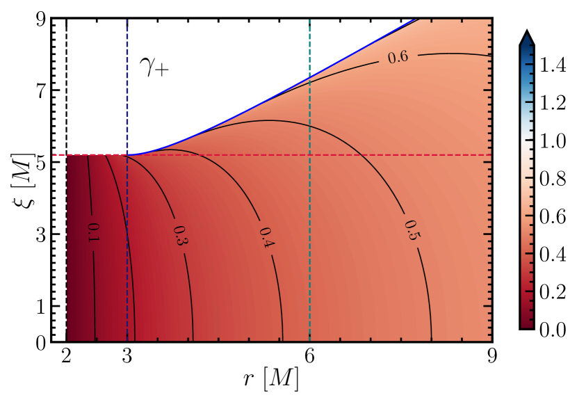
Figure 11: Here we show the redshifts $\gamma_{\pm}$ experienced by photons that reach asymptotic observers, depending on where they were emitted from ($x$-axis) and in which way they were moving initially, i.e., whether they were emitted toward the BH ($-$) or away from it ($+$). As expected, only radially-ingoing photons experience blueshifts, and photons emitted close to the horizon experience infinite redshifts. The vertical and horizontal lines have the same meaning as in Fig. 10.

The left panel of Fig. 10 shows characteristic sample values of conserved quantities $\xi$ and starting positions $r$ from which emitted photons can reach asymptotic observers, and thus participate in image formation (shown in orange lines). These can be distributed into two sets based whether they have a radially-ingoing leg ($\xi>\xi_{\text{ps}}$) or not ($\xi<\xi_{\text{ps}}$). This simple schematic then immediately makes clear the logic behind writing the key equation we have used here, Eq. 12. Ingoing photons with impact parameters larger than that of the photon on the CNG, $\xi>\xi_{\text{ps}}$, and emitted far away from the BH “turn” at the outer turning point $r_{\text{tp-0}}$ and start moving radially-outwards whereas those that are initially outgoing and emitted near the horizon fall back onto the BH since these are reflected at the inner turning point $r_{\text{tp-1}}$. The expressions for both these quantities (shown in blue in the figure) are given as,

$$r_{\text{tp-k}}(\xi)=\frac{2\xi}{\sqrt{3}}\cos{\left[\frac{1}{3}\cos^{-1}{\left(-\frac{\xi_{\text{ps}}}{\xi}\right)}-\frac{2\pi k}{3}\right]}\,.$$ (29)

The right panel of Fig. 10 shows the modulus of the inverse radial velocity $\Lambda=|1/k_{\pm,\pm}^{r}|$ of photons moving through the Schwarzschild spacetime. This factor is one of the two purely emission-independent pieces in the intensity integral (12), and the bright yellow region shows where this term contributes the most, i.e., close to the orbit’s turning point- where its radial velocity is the smallest. Equivalently, this is where the affine-time along the null geodesic per unit radius (and thus the amount of intensity contributed to the null geodesic, when a source of emission is present) is the largest.

In Fig. 11, we display the variation in the redshifts experienced by ingoing (-) and outgoing photons emitted with an impact parameter $\xi$ at a radius $r$. We highlight the change in $\gamma_{-}$ from representing a blueshift ($>1$) to a redshift close to the turning point of a photon orbit (due to reduced radial velocity).

References

- Abdujabbarov et al. (2015) Abdujabbarov A. A., Rezzolla L., Ahmedov B. J., 2015, MNRAS, 454, 2423
- Bambi (2013) Bambi C., 2013, Phys. Rev. D, 87, 107501
- Bambi & Modesto (2013) Bambi C., Modesto L., 2013, Phys. Lett. B, 721, 329
- Bardeen (1974) Bardeen J. M., 1974, in Dewitt-Morette C., ed., Vol. 64, Gravitational Radiation and Gravitational Collapse. p. 132
- Bauer et al. (2021) Bauer A., Cárdenas-Avendaño A., Gammie C. F., Yunes N., 2021, arXiv e-prints, p. arXiv:2111.02178
- Broderick et al. (2014) Broderick A. E., Johannsen T., Loeb A., Psaltis D., 2014, ApJ, 784, 7
- Broderick et al. (2021) Broderick A. E., Tiede P., Pesce D. W., Gold R., 2021, arXiv e-prints, p. arXiv:2105.09962
- Event Horizon Telescope Collaboration et al. (2019a) Event Horizon Telescope Collaboration et al., 2019a, ApJ Lett., 875, L1
- Event Horizon Telescope Collaboration et al. (2019b) Event Horizon Telescope Collaboration et al., 2019b, ApJ Lett., 875, L2
- Event Horizon Telescope Collaboration et al. (2019c) Event Horizon Telescope Collaboration et al., 2019c, ApJ Lett., 875, L3
- Event Horizon Telescope Collaboration et al. (2019d) Event Horizon Telescope Collaboration et al., 2019d, ApJ Lett., 875, L4
- Event Horizon Telescope Collaboration et al. (2019e) Event Horizon Telescope Collaboration et al., 2019e, ApJ Lett., 875, L5
- Event Horizon Telescope Collaboration et al. (2019f) Event Horizon Telescope Collaboration et al., 2019f, ApJ Lett., 875, L6
- Gan et al. (2021) Gan Q., Wang P., Wu H., Yang H., 2021, Phys. Rev. D, 104, 024003
- Garfinkle et al. (1991) Garfinkle D., Horowitz G. T., Strominger A., 1991, Phys. Rev. D, 43, 3140
- Gebhardt et al. (2011) Gebhardt K., Adams J., Richstone D., Lauer T. R., Faber S. M., Gültekin K., Murphy J., Tremaine S., 2011, ApJ, 729, 119
- Gibbons & Maeda (1988) Gibbons G. W., Maeda K.-I., 1988, Nuc. Phys. B, 298, 741
- Gimeno-Soler et al. (2019) Gimeno-Soler S., Font J. A., Herdeiro C., Radu E., 2019, Phys. Rev. D, 99, 043002
- Gralla (2021) Gralla S. E., 2021, Phys. Rev. D, 103, 024023
- Gralla et al. (2019) Gralla S. E., Holz D. E., Wald R. M., 2019, Phys. Rev. D, 100, 024018
- Hioki & Maeda (2009) Hioki K., Maeda K.-I., 2009, Phys. Rev. D, 80, 024042
- Jaroszynski & Kurpiewski (1997) Jaroszynski M., Kurpiewski A., 1997, A&A, 326, 419
- Johannsen et al. (2016) Johannsen T., Wang C., Broderick A. E., Doeleman S. S., Fish V. L., Loeb A., Psaltis D., 2016, Phys. Rev. Lett., 117, 091101
- Johnson et al. (2020) Johnson M. D., et al., 2020, Science Adv., 6, eaaz1310
- Jusufi et al. (2021) Jusufi K., Saurabh K., Azreg-Aïnou M., Jamil M., Wu Q., Bambi C., 2021, arXiv e-prints, p. arXiv:2106.08070
- Kocherlakota & Rezzolla (2020) Kocherlakota P., Rezzolla L., 2020, Phys. Rev. D, 102, 064058
- Kocherlakota et al. (2021) Kocherlakota P., et al., 2021, Phys. Rev. D, 103, 104047
- Kocherlakota et al. (2022) Kocherlakota P., Rezzolla L., Wielgus M., 2022, in preparation
- Konoplya et al. (2016) Konoplya R., Rezzolla L., Zhidenko A., 2016, Phys. Rev. D, 93, 064015
- Lara et al. (2021) Lara G., Völkel S. H., Barausse E., 2021, arXiv e-prints, p. arXiv:2110.00026
- Mazur & Mottola (2004) Mazur P. O., Mottola E., 2004, PNAS, 101, 9545
- Medeiros et al. (2020) Medeiros L., Psaltis D., Özel F., 2020, ApJ, 896, 7
- Mizuno et al. (2018) Mizuno Y., et al., 2018, Nature Astronomy, 2, 585
- Narayan et al. (2019) Narayan R., Johnson M. D., Gammie C. F., 2019, ApJ Lett., 885, L33
- Olivares et al. (2020) Olivares H., et al., 2020, MNRAS, 497, 521
- Ozel et al. (2021) Ozel F., Psaltis D., Younsi Z., 2021, arXiv e-prints, p. arXiv:2111.01123
- Psaltis et al. (2020) Psaltis D., Medeiros L., Christian P., Ozel F., the EHT Collaboration 2020, Phys. Rev. Lett., 125, 141104
- Pu & Broderick (2018) Pu H.-Y., Broderick A. E., 2018, ApJ, 863, 148
- Rezzolla & Zhidenko (2014) Rezzolla L., Zhidenko A., 2014, Phys. Rev. D, 90, 084009
- Sen (1992) Sen A., 1992, Phys. Rev. Lett., 69, 1006
- Shaikh & Joshi (2019) Shaikh R., Joshi P. S., 2019, JCAP, 10, 064
- Shaikh et al. (2019) Shaikh R., Kocherlakota P., Narayan R., Joshi P. S., 2019, Mon. Not. R. Astron. Soc., 482, 52
- Suvorov (2020) Suvorov A. G., 2020, Class. Quant. Grav., 37, 185001
- The Ligo Scientific Collaboration et al. (2021) The Ligo Scientific Collaboration the VIRGO Collaboration the KAGRA Collaboration 2021, ApJ, 915, L5
- Völkel & Barausse (2020) Völkel S. H., Barausse E., 2020, Phys. Rev. D, 102, 084025
- Völkel et al. (2021) Völkel S. H., Barausse E., Franchini N., Broderick A. E., 2021, Class. Quantum Grav., 38, 21LT01
- Will (2006) Will C. M., 2006, Liv. Rev. Relativ., 9, 3
- Yang et al. (2021) Yang S., Liu C., Zhu T., Zhao L., Wu Q., Yang K., Jamil M., 2021, Chin. Phys. C, 45, 015102
- Younsi et al. (2012) Younsi Z., Wu K., Fuerst S. V., 2012, A&A, 545, A13
- Younsi et al. (2016) Younsi Z., Zhidenko A., Rezzolla L., Konoplya R., Mizuno Y., 2016, Phys. Rev. D, 94, 084025
- Younsi et al. (2021) Younsi Z., Psaltis D., Özel F., 2021, arXiv e-prints, p. arXiv:2111.01752
- Yuan & Narayan (2014) Yuan F., Narayan R., 2014, ARAA, 52, 529