When less is more: Simplifying inputs aids neural network understanding

Abstract

How do neural network image classifiers respond to simpler and simpler inputs? And what do such responses reveal about the learning process? To answer these questions, we need a clear measure of input simplicity (or inversely, complexity), an optimization objective that correlates with simplification, and a framework to incorporate such objective into training and inference. Lastly we need a variety of testbeds to experiment and evaluate the impact of such simplification on learning. In this work, we measure simplicity with the encoding bit size given by a pretrained generative model, and minimize the bit size to simplify inputs in training and inference. We investigate the effect of such simplification in several scenarios: conventional training, dataset condensation and post-hoc explanations. In all settings, inputs are simplified along with the original classification task, and we investigate the trade-off between input simplicity and task performance. For images with injected distractors, such simplification naturally removes superfluous information. For dataset condensation, we find that inputs can be simplified with almost no accuracy degradation. When used in post-hoc explanation, our learning-based simplification approach offers a valuable new tool to explore the basis of network decisions.

1 Introduction

A better understanding of the information deep neural networks use to learn can lead to new scientific discoveries (Raghu & Schmidt, 2020), highlight differences between human and model behaviors (Makino et al., 2020) and serve as powerful auditing tools (Geirhos et al., 2020; D’souza et al., 2021; Bastings et al., 2021; Agarwal et al., 2021).

Removing information from the input deliberately is one way to illuminate what information content is relevant for learning. For example, occluding specific regions, or removing certain frequency ranges from the input gives insight into which input regions and frequency ranges are relevant for the network’s prediction (Zintgraf et al., 2017; Makino et al., 2020; Banerjee et al., 2021a). These ablation techniques use simple heuristics such as random removal (Hooker et al., 2019; Madsen et al., 2021), or exploit domain knowledge about interpretable aspects of the input to create simpler versions of the input on which the network’s prediction is analyzed (Banerjee et al., 2021b).

What if, instead of using heuristics, one learns to synthesize simpler inputs that retrain prediction-relevant information? This way, we could gain intuition into the model behavior without relying on prior or domain knowledge about what input content may be relevant for the network’s learning target. To achieve this, one needs to define the precise meaning of “simplifying an input”, including direct metrics for such simplification and retention of task-relevant information.

In this work, we propose SimpleBits, an information-reduction method that learns to synthesize simplified inputs which contain less information while remaining informative for the task. To measure simplicity, we use a finding initially reported as a problem for density-based anomaly detection—that generative image models tend to assign higher probability densities and hence lower bits to visually simpler inputs (Kirichenko et al., 2020; Schirrmeister et al., 2020). However, we use this to our advantage and minimize the encoding bit size given by a generative network trained on a general image distribution to simplify inputs. At the same time, we optimize for the original task so that the simplified inputs still preserve task-relevant information.

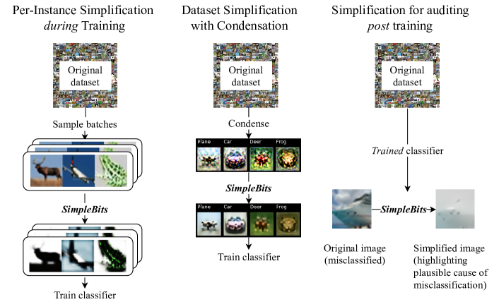
Figure 1: We apply SimpleBits to a variety of tasks to aid neural network understanding. Left: SimpleBits acts as a per-instance simplifier during training, where each image is simplified but the total number of images remain the same. Center: SimpleBits is combined with data condensation techniques, to reduce both the size of the dataset and the complexity of individual images in the condensed dataset. Right: SimpleBits is used as a post-hoc analysis tool of any trained classifier, illuminating features of images that are crucial to the network’s decision.

We apply SimpleBits both in a per-instance setting, where each image is processed to be a simplified version of itself, and the size of training set remains unchanged, as well as in a condensation setting, where the dataset is compressed to only a few samples per class, with the condensed samples simplified at the same time. Applied during training, SimpleBits can be used to investigate the trade-off between the information content and the task performance. Post training, SimpleBits can act as an analysis tool to understand what information a trained model uses for its decision making. Figure 1 summarizes the tasks covered in this paper.

Our evaluation provides the following insights in the investigated scenarios:

1. Per-instance simplification during training. SimpleBits successfully removes superfluous information for tasks with injected distractors. On natural image datasets, SimpleBits highlights plausible task-relevant information (shape, color, texture). Increasing simplification leads to accuracy decreases, as expected, and we report the trade-off between input simplification and task performance for different datasets and problems.

2. Dataset simplification with condensation. We evaluate SimpleBits applied to a condensation setting where the training data are converted into a much smaller set of synthetic images. SimpleBits further simplifies these images to drastically reduce the encoding size without substantial task performance decrease. On a chest radiograph dataset (Johnson et al., 2019a, b), SimpleBits can uncover known radiologic features for pleural effusion and gender.

3. Simplification for auditing post-training. Given a trained classifier on regular datasets, we explore the use of SimpleBits as an interpretability tool for auditing processes. Our exploration of SimpleBits guided audits suggests it can provide intuition into model behavior on individual examples, including finding features that may contribute to misclassifications.

Figure 2: Visualization of the bits-per-dimension ($\mathrm{bpd}$) measure for image complexity, sorted from low to high. Image samples are taken from MNIST, Fashion-MNIST, CIFAR10 and CIFAR100, in addition to a completely black image sample. $\mathrm{bpd}$ is calculated from the density produced by a Glow (Kingma & Dhariwal, 2018) model pretrained on 80 Million Tiny Images. Switching to other types of generative models including PixelCNN and diffusion models trained on other datasets produces consistent observations; see Figure S1 in Supplementary Information for more details.

2 Measuring and Reducing Instance Complexity

How to define simplicity? We use the fact that generative image models tend to assign lower encoding bit sizes to visually simpler inputs (Kirichenko et al., 2020; Schirrmeister et al., 2020). Concretely, the complexity of an image $\bm{x}$ can be quantified as the negative log probability mass given by a pretrained generative model with tractable likelihood, $G$, i.e. $-\log p_{G}(\bm{x})$. $-\log p_{G}(\bm{x})$ can be interpreted as the image encoding size in bits per dimension (bpd) via Shannon’s theorem (Shannon, 1948): $\textrm{bpd}(\bm{x})=-\log_{2}p_{G}(\bm{x})/d$ where $d$ is the dimension of the flattened $\bm{x}$.

The simplification loss for an input $\bm{x}$, given a pre-trained generative model $G$, is as follows:

$$\eqparbox[t]{A}{$\displaystyle L_{\mathrm{sim}}$\hfil}(\bm{x}) =-\log p_{G}(\bm{x})$$ (1)

Figure 2 visualizes images and their corresponding bits-per-dimension ($\mathrm{bpd}$) values given by a Glow network (Kingma & Dhariwal, 2018) trained on 80 Million Tiny Images (Torralba et al., 2008) (see Supplementary Section S1 for other models). This is the generative network used across all our experiments. A visual inspection of Figure 2 suggests that lower $\mathrm{bpd}$ corresponds with simpler inputs, as also noted in prior work (Serrà et al., 2020). The goal of our approach, SimpleBits, is to minimize $\mathrm{bpd}$ of input images while preserving task-relevant information.

We now explore how SimpleBits affects network behavior in a variety of scenarios. In each scenario, we explain the method to optimize $L_{\mathrm{sim}}$ and the retention of task-relevant information, the experimental setup, and results. All code is at https://tinyurl.com/simple-bits.

3 Per-instance simplification during training

When plugged into the training of a classifier $f$, SimpleBits simplifies each image such that $f$ can still learn the original classification task from the simplified batches. We apply backpropagation through training steps: given a batch of input images $\bm{X}_{\mathrm{orig}}$, before updating the classifier $f$, an image-to-image $\mathrm{simplifier}$ network generates a corresponding batch of images $\bm{X}_{\mathrm{sim}}$ such that: (a) images in $\bm{X}_{\mathrm{sim}}$ have low $\mathrm{bpd}$ as measured per $L_{\mathrm{sim}}$ in  Equation (1), and (b) training on the simplified images leads to a reduction of the classification loss on the original images.

We optimize (b) by unrolling one training step of the classifier. So for a single batch $\bm{X}_{\mathrm{orig}},\bm{y}$, we first compute an updated classifier $f^{\prime}$ as follows:

$$\eqparbox[t]{A}{$\displaystyle\bm{X}_{\mathrm{sim}}$\hfil} =\mathrm{simplifier}(\bm{X}_{\mathrm{orig}})$$ (2)

$$\eqparbox[t]{A}{$\displaystyle f^{\prime}$\hfil} =\mathrm{train\_step}(f,l(f(\bm{X}_{\mathrm{sim}}),\bm{y}))$$ (3)

where $\mathrm{simplifier}$ is an image-to-image network, $l$ is the classification loss function, i.e., the cross-entropy loss, and $f^{\prime}$ is the classifier $f$ after one optimization step using the classification loss $l(f(\bm{X}_{\mathrm{sim}}),\bm{y})$ on the simplified data.

To train the $\mathrm{simplifier}$ network, we optimize for both (a) (Equation (1)) and for the classification loss on the batch of original images with the updated classifier after the unrolled training step $l(f^{\prime}(\bm{X}_{\mathrm{orig}}),\bm{y})$ using backpropagation through training (Maclaurin et al., 2015; Finn et al., 2017). Note that one could not instead directly optimize performance on the simplified images as the simplifier could then collapse all simplified images of one class to one representative example.

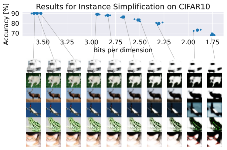
Figure 3: Selection of SimpleBits applied to CIFAR10 training images. Simplified images from settings with varying simplification loss weight $\lambda_{\textrm{sim}}$. We observe that at lower bits per dimension color is retained only for some images such as green color for frog or blue sky for the plane. In this low bit regime, texture remains discernable for the cat and frog images. More simplified images are in Section S8.

Adding the classification losses on the simplified data both before and after the unrolled training step ensures the training is not influenced by predictions on the simplified data that are very different from the classification target and we found that to improve training stability, leading to:

$$\eqparbox[t]{A}{$\displaystyle L_{\mathrm{cls}}$\hfil} =l(f^{\prime}(\bm{X}_{\mathrm{orig}}),\bm{y})+l(f(\bm{X}_{\mathrm{sim}}),\bm{y})+l(f^{\prime}(\bm{X}_{\mathrm{sim}}),\bm{y})$$ (4)

Further details to stabilize the training are described in Supplementary S3. The total loss for the $\mathrm{simplifier}$ is

$$L =\lambda_{\textrm{sim}}\cdot L_{\mathrm{sim}}+L_{cls},$$ (5)

where $\lambda_{\textrm{sim}}$ is a hyperparameter for the trade-off between simplification and task performance. In subsequent experiments, we vary $\lambda_{\textrm{sim}}$ to control the extent of simplification.

Implementation Our training architecture is a normalizer-free classifier architecture to avoid interpretation difficulties that may arise from normalization layers, such as image values being downscaled by the $\mathrm{simplifier}$ and then renormalized again. We use Wide Residual Networks as described by Brock et al. (2021) for the classifier. The normalizer-free architecture reaches 94.0% on CIFAR10 in our experiments, however we opt for a smaller variant for faster experiments that reaches 91.2%; additional details are included in the Supplementary Section S2.1. For the $\mathrm{simplifier}$ network, we use a UNet architecture (Ronneberger et al., 2015) that we modify to be residual, more details included in Supplementary Section S2.2. For both $\mathrm{simplifier}$ and classifier networks, we use AdamW (Loshchilov & Hutter, 2019) with $\mathrm{lr}=5\cdot 10^{-4}$ and $\mathrm{weight\_decay}=10^{-5}$.

3.1 SimpleBits Removes Injected Distractors

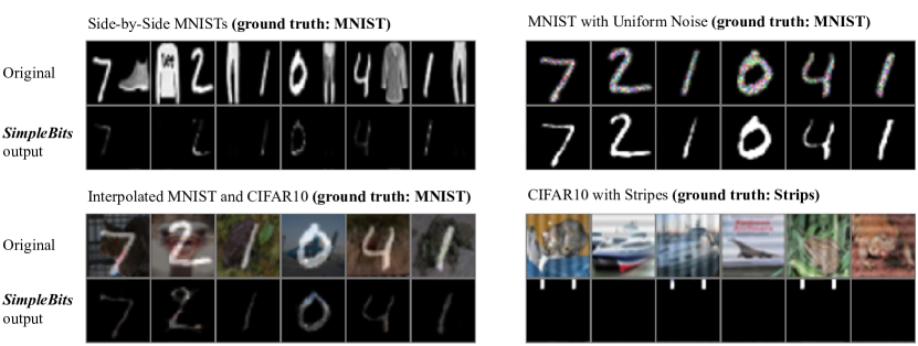
Figure 4: Evaluation of SimpleBits as a distractor removal on four composite datasets. Shown are the composite original images and the corresponding simplified images produced by SimpleBits trained alongside the classifier. SimpleBits is able to almost entirely remove task-irrelevant image parts, namely FashionMNIST (top left), random noise (top right), CIFAR10 (bottom left as well as bottom right).

We first evaluate whether our per-instance simplification during training successfully removes superfluous information for tasks with injected distractors. To that end, we construct datasets to contain both useful (ground truth) and redundant (distractor) information for task learning. We create four composite datasets derived from three conventional datasets: MNIST (LeCun & Cortes, 2010), FashionMNIST  (Xiao et al., 2017) and CIFAR10 (Krizhevsky, 2009). Sample images, both constructed (input to the whole model) and simplified (output of $\mathrm{simplifier}$ and input to classifier), are shown in Figure 4.

Side-by-Side MNIST constructs each image by horizontally concatenating one image from Fashion-MNIST and one from MNIST. Each image is rescaled to 16x32, so the concatenated image size remains 32x32; the order of concatenation is random. The ground truth target is MNIST labels, and therefore FashionMNIST is an irrelevant distractor for the classification task. As seen in Figure 4, the $\mathrm{simplifier}$ effectively removes the clothes side of the image.

MNIST with Uniform Noise adds uniform noise to the MNIST digits, preserving the MNIST digit as the classification target. Hence the noise is the distractor and is expected to be removed. And indeed the noise is no longer visible in the simplified outputs shown in Figure 4.

Interpolated MNIST and CIFAR10 is constructed by interpolating between MNIST and CIFAR10 images. MNIST digits are the classification target. The expectation is that the simplified images should no longer contain any of the CIFAR10 image information. The result shows that most of the CIFAR10 background is removed, leaving only slight traces of colors.

CIFAR10 with Stripes overlays either horizontal or vertical stripes onto CIFAR10 images, with the binary classification label 0 for horizontal and 1 for vertical stripes. With this dataset we observe the most drastic and effective information removal, where only the tip of vertical strips is retained, which by itself is sufficient to solve this binary classification task.

Figure 5: Results for training image simplifications on real datasets. Dots show results for training with different loss weights for the simplification loss. Images with less bits per dimension lead to reduced accuracies, and such reduction is more pronounced for complex datasets like CIFAR10.

3.2 Trade-off Curves on Conventional Datasets

We verified that SimpleBits is able to discern information relevance in inputs, and effectively removes redundant content to better serve the classification task. In real-world datasets, however, the type, as well as the amount of information redundancy in inputs is often unclear.

With the same framework, by varying the simplification weight $\lambda_{\textrm{sim}}$ we can study the trade-off between task performance and level of simplification to better understand a given dataset. On one end, with $\lambda_{\textrm{sim}}=0$ it should faithfully restores to conventional training. On the other end, when $\lambda_{\textrm{sim}}$ is sufficiently high (resulting in an all-black input image), the training is expected to fail.

We experimented with MNIST, Fashion-MNIST, SVHN (Netzer et al., 2011) and CIFAR10, producing a trade-off curve for each by setting the strength of the simplification loss to various values during training, including $\lambda_{\textrm{sim}}=0$. For each setting, we report the classification accuracy as a result of joint training of simplification and classification, retraining from scratch with only simplified images, and finetuning after joint training with simplified images, respectively, as shown in Figure 5.

As expected, higher strengths of simplification lead to decreased task performance. Interestingly, such decay is observed to be more pronounced for more complex datasets such as CIFAR10. This suggests either the presence of a relatively small amount of information redundancy, or that naturally occurring noise in data helps with generalization, analogous to how injected noise from data augmentation helps learning features invariant to translations and viewpoints, even though the augmentation itself does not contain additional discriminative information.

We run three baselines to validate the efficacy of our simplification framework, as described in Supplementary Section S7 and shown in Figure S4. Section S5 shows that our simplification has practical savings in image storage. More analyses including training curves and potential spurious features revealed by SimpleBits can be seen in Supplementary Section S6 and S9, respectively.

4 Dataset simplification with Condensation

Now we investigate how SimpleBits affects training on a small synthetic condensed dataset. Multiple methods have been developed for dataset condensation (Zhao et al., 2021; Zhao & Bilen, 2021; Wang et al., 2018; Maclaurin et al., 2015), via backpropagation through training (Wang et al., 2018; Maclaurin et al., 2015), gradient matching (Zhao & Bilen, 2021), or kernel based meta-learning (Nguyen et al., 2021). Due to its small size, one can visualize the full condensed dataset to understand what information is preserved for learning. Our aim here is to combine SimpleBits with dataset condensation to see if we could obtain a both smaller and simpler training dataset than the original.

In this setting, we jointly condense our training dataset to a smaller number of synthetic training inputs and simplify the synthetic inputs according to our simplification loss (Eq. 1). Concretely, we add the simplification loss $L_{\mathrm{sim}}$ to the gradient matching loss proposed by Zhao & Bilen (2021). The gradient matching loss computes the layerwise cosine distance between the gradient of the classification loss wrt. to the classifier parameters $\theta$ produced by a batch of original images $\bm{X}_{\mathrm{orig}}$ and a batch of synthetic images $\bm{X}_{\mathrm{syn}}$:

$$\begin{split}&L_{\textrm{match}}(\bm{X}_{\mathrm{orig}},\bm{X}_{\mathrm{syn}})=\\ &D(\nabla_{\theta}l(f(\bm{X}_{\mathrm{orig}}),\bm{y}),\nabla_{\theta}l(f(\bm{X}_{\mathrm{syn}}),\bm{y})).\end{split}$$ (6)

where $D$ is the layerwise cosine distance. The matching loss is computed separately per class.

Overall, with our simplification loss, we get:

$$\begin{split}L_{\mathrm{syn}}(\bm{X}_{\mathrm{orig}},\bm{X}_{\mathrm{syn}})=&\ L_{\mathrm{match}}(\bm{X}_{\mathrm{orig}},\bm{X}_{\mathrm{syn}})\\ &+\sum_{\bm{x}_{\mathrm{syn}}\in\bm{X}_{\mathrm{syn}}}-\log{p_{G}(\bm{x}_{\mathrm{syn}})}\end{split}$$ (7)

We perform dataset condensation on MNIST, Fashion-MNIST, SVHN and CIFAR10 with varying $\lambda_{\textrm{sim}}$ for the simplification loss. We also apply dataset condensation to the chest radiograph dataset MIMIC-CXR-JPG (Johnson et al., 2019a, b) for predicting pleural effusion and gender. We use the networks from (Zhao et al., 2021), but use Adam (Kingma & Ba, 2015) for optimization.

4.1 SimpleBits retains condensation performance while greatly simplifying data

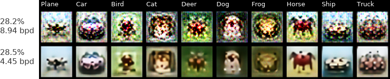
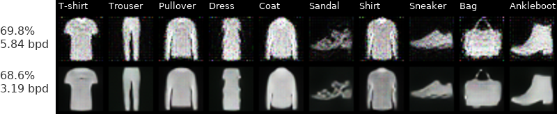
Figure 6: Dataset condensation accuracies (when retraining with the condensed dataset) vs. data simplicity. Top: Each dot represents a data condensation experiment run with a particular weight for the simplification loss, which results in more or less complex datasets. Accuracies can be retained even with substantially reduced bits per dimension. In the 1-image-per-class case (top left figure), arrows highlight the settings that are visualized in the bottom figure. Bottom: Condensed datasets with varying simplification loss weight. Each row represents the whole condensed dataset (1 image per class), with high (top row) or low (bottom row) bits per dimension. Lower bits per dimension datasets are visually simpler and smoother while retaining the accuracy.

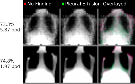
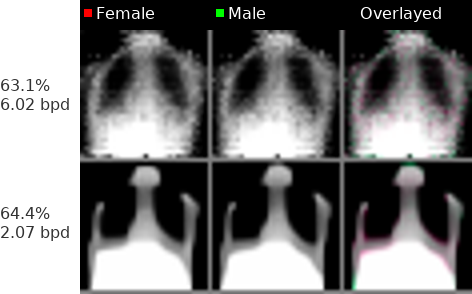
Figure 7: Condensed dataset for pleural effusion and gender prediction from chest radiographs in MIMIC-CXR. Condensed images for the classes look very similar. Color-coded mixed rightmost images reveal the differences between the classes. Green highlighted region at the lower end of the lung consistent with typical radiologic features for pleural effusion (white region indicating fluid on lungs), red highlighted around lung for gender indicate smaller lung volume for the female class.

In Figure 6, we examine the accuracy for each condensed-and-simplified dataset. We observe that for the natural image datasets, accuracies are mostly retained when decreasing the number of bits per image. Note that the setting with highest bpd is a reimplementation of Zhao et al. (2021) and therefore a baseline without simplification loss. We visualize examples in Figure 6 and observe that the jointly condensed and simplified images look visually smoother, indicating that higher frequency patterns visible in the original images are not needed to reach the same accuracy. These visualizations are also noticeably more smooth than the results for per-instance simplification Figure 4, which suggests that data condensation may already favor features that are less complex. Further condensed sets are in Section S10 and a continual learning evaluation in S11.

Evaluation of a medical chest radiograph dataset We also evaluate jointly condensing and simplifying for a dataset of chest radiograph images (Johnson et al., 2019a, b). This dataset has known radiologic features for the presence of pleural effusion (Jany & Welte, 2019; Raasch et al., 1982) and difference in gender (Bellemare et al., 2003). In Figure 7, we visualize both the condensed (top row) and the jointly condensed and simplified dataset (bottom row). The overlayed shows that a visible difference between presence of feature. For pleural effusion, a larger white region on the bottom of the lung occurs in the simplified pathological image, while for gender, lungs appear slightly smaller for the simplified female image.

5 Post-training simplification

Algorithm 1 Simplification loss function after training

  given generative network $G$, input $\bm{x}_{\mathrm{orig}}$, simplified input $\bm{x}_{\mathrm{sim}}$, classifier $f$, parameter scaling factors $\bm{s}<1$

  Scale classifier parameters down by $\bm{s}$ to simulate "forgetting"

  $f_{\mathrm{scd}}\leftarrow\text{ScaleParameters}(f,\bm{s})$

  Predict original and simplified with unscaled classifier

  $\bm{h}_{\mathrm{orig}}=f(\bm{x}_{\mathrm{orig}}),\bm{h}_{\mathrm{sim}}=f(\bm{x}_{\mathrm{sim}})$

  Predict original and simplified with scaled classifier

  $\bm{h}_{\mathrm{orig,scd}}=f_{\mathrm{scd}}(\bm{x}_{\mathrm{orig}}),\bm{h}_{\mathrm{sim,scd}}=f_{\mathrm{scd}}(\bm{x}_{\mathrm{sim}})$

  Compute gradients of prediction divergence wrt. scaling factors

  $grad_{\mathrm{orig}}=\nabla_{\bm{s}}D_{\mathrm{KL}}(\bm{h}_{\mathrm{orig}}\|\bm{h}_{\mathrm{orig,scd}})$

  $grad_{\mathrm{sim}}=\nabla_{\bm{s}}D_{\mathrm{KL}}(\bm{h}_{\mathrm{orig}}\|\bm{h}_{\mathrm{sim,scd}})$

  Compute layerwise cosine distance between gradients

  $L_{\mathrm{grad}}=D_{\mathrm{cos}}(grad_{\mathrm{orig}},grad_{\mathrm{sim}})$

  Compute prediction differences of original and simplified

  $L_{\mathrm{pred}}=D_{\mathrm{KL}}(\bm{h}\|\bm{h}_{\mathrm{sim}})+D_{\mathrm{KL}}(\bm{h}_{\mathrm{scd}}\|\bm{h}_{\mathrm{sim,scd}})$

  Compute needed bits for simplified input

  $L_{\mathrm{sim}}=-\log p_{G}(\bm{x}_{\mathrm{sim}}))$

  return $L_{\mathrm{grad}}+L_{\mathrm{pred}}+\lambda_{\mathrm{sim}}\cdot L_{\mathrm{sim}}$

Can SimpleBits be used to interpret trained classifiers after training? We explore simplifying images post-training as a basis for gaining intuition about model behavior. We will do so by using SimpleBits to visualize some of the information that would help the classifier remember what it has learned for a specific prediction.

For synthesizing the prediction-relevant information, we simulate that the classifier forgets knowledge and then synthesize a simplified input that allows the classifier to relearn the relevant knowledge for the prediction of the original input. To simulate forgetting, we scale down all parameters of the trained classifier $f$ by multiplying them with a gating value $\phi_{\textrm{scaled},i}=\phi_{i}\cdot s,s<1$. This scaling removes information from the model by bringing the learned parameter values closer to zero, is identical to weight decay and also makes the network simpler in terms of model encoding size (Hinton & van Camp, 1993). To synthesize a simplified input that helps learning to restore the parameter values that are important for a specific input, we compare gradients between the original and simplified input.

Given an input, we can compute the gradients of the KL-divergence between the rescaled network’s prediction $f_{\mathrm{scd}}(x)$ and the original network’s prediction $f(x)$. At each iteration, the layerwise cosine distance between these two sets of gradients (one for original datapoint and the other for the simplified) is the basis of the loss used in SimpleBits. We compute this distance only considering the gradients that are negative for the original input. Combined with the simplification loss Eq. 1, this amounts to asking what input information is needed to recover parts of the original network to restore the original prediction? To ensure that the network is trained towards minimizing the same prediction difference on the simplified and original data, we also add a prediction difference loss $L_{\textrm{pred}}$. Further details about the implementation are included in Alg. 1 and Supplementary Section S4. We use the loss computed in Alg. 1 to optimize the latent encoding of the simplified image with Adam.

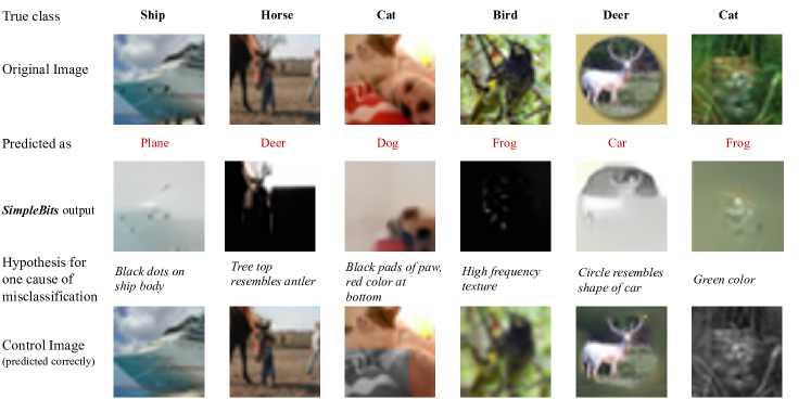
Figure 8: Post-hoc simplifications of misclassified CIFAR-10 examples. For each example, the simplified image reveals plausible causes for the misclassification. We subsequently made alterations to compensate for the cause (from left to right: removing black dots, removing tree top, removing color, removing high frequency texture, removing circle, and removing color), and are able to revert the predictions to the true class.

In Figure 8, we visualize both the misclassified images according to the original network $f$ and produce the corresponding simplified versions. We observe that simplified images may provide some intuition into the reason for the network’s misclassification, highlighting a variety of different features for different images. We imagine a possible practitioner workflow, where the practitioner derives a set of possible hypotheses for the misclassification from SimpleBits and tests them on the real data. We show further post-hoc simplified examples and a comparison to saliency-based methods in supplementary Section S12.

6 Related Work

Our approach simplifying individual training images builds on Raghu et al. (2021), where they learn to inject information into the classifier training. Per-instance simplification during training can be seen as a instance of their framework combined with the idea of input simplification. In difference to their methods, SimpleBits explicitly aims for interpretability through input simplification.

Other interpretability approaches that synthesize inputs include generating counterfactual inputs (Hvilshøj et al., 2021; Dombrowski et al., 2021; Goyal et al., 2019) or inputs with exaggerated features (Singla et al., 2020). SimpleBits differs in explicitly optimizing the inputs to be simpler.

Generative models have often been used in various ways for interpretability such as generating realistic-looking inputs (Montavon et al., 2018) and by directly training generative classifiers (Hvilshøj et al., 2021; Dombrowski et al., 2021), but we are not aware of any work except (Dubois et al., 2021) (discussed above) to explicitly generate simpler inputs. A different approach to reduce input bits while retaining classification performance is to train a compressor that only keeps information that is invariant to predefined label-preserving augmentations. Dubois et al. (2021) implement this elegant approach in two ways. In their first variant, by training a VAE to reconstruct an unaugmented input from augmented (e.g. rotated, translated, sheared) versions. In their second variant, building on the CLIP (Radford et al., 2021) model, they view images with the same associated text captions as augmented versions of each other. This allows the use of compressed CLIP encodings for classification and achieves up to 1000x compression on Imagenet without decreasing classification accuracy. Their approach focuses on achieving maximum compression while our approach is focused on interpretability. Their approach requires access to predefined label-preserving augmentations and has reduced classification performance in input space compared to latent/encoding space.

7 Conclusion

We propose SimpleBits, an information-based method to synthesize simplified inputs. Crucially, SimpleBits does not require any domain-specific knowledge to constrain or dictate which input components should be removed; instead SimpleBits itself learns to remove the components of inputs which are least relevant for a given task.

As an interpretability tool, we show that SimpleBits is able to remove injected distractors, suggest plausible reasons for misclassification, and recover known radiologic features from condensed datasets. When combined with data condensation, SimpleBits retains accuracy while greatly reducing the complexity of condensed images.

Our simplification approach sheds light on the amount of information required for a deep network classifier to learn its task. We find that the tradeoff between task performance and input simplification varies by dataset and setting — it is more pronounced for more complex datasets.

Reproducibility Statement

We provide the following information to ensure reproducibility. Main concepts, algorithms and basic architectures are described in Sections 3, 5 and 4. Further network architecture details are in Supplementary Sections S2.1 and S2.2, further optimization details in Supplementary Sections S3 and S4. Finally, the code is available under https://tinyurl.com/simple-bits.

 

Supplementary Information for:
When less is more: Simplifying inputs aids neural network understanding

 

Supplementary outline

This document completes the presentation of the main paper with the following:

Supplementary Section	Type of content	Relevant section in main text	TL;DR
S1	Additional experiments	Section 2	Example images with $\mathrm{bpd}$ values produced by other generative models
S2, S3	Implementation details	Section 3	Architecture and optimization details for simplification during training
S4	Implementation details	Section 5	Optimization details post-hoc simplification
S5, S6, S7	Additional experiments	Section 3.2	Baselines, training curves, file size analysis
S8	More figures	Figure 3	Uncurated sets of simplified images at end of joint training
S9	Additional findings	Section 3.2	Potential spurious features revealed by SimpleBits
S10	More figures	Section 4	More simplified condensed dataset images
S11	Additional experiments	Section 4	Simplified condensed datasets evaluated in a continual learning setting
S12	Additional findings	Section 5	More use cases of post-training auditing, with comparison to saliency-based methods

Appendix S1 BPDs of other generative models

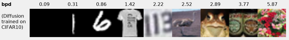
Figure S1: Visualization of the bits-per-dimension ($\mathrm{bpd}$) measure for image complexity, sorted from low to high. Image samples are taken from MNIST, Fashion-MNIST, CIFAR10 and CIFAR100, in addition to a completely black image sample. $\mathrm{bpd}$ is calculated from the density produced by a Glow (Kingma & Dhariwal, 2018) model pretrained on 80 Million Tiny Images, a PixelCNN model trained on CIFAR10, and a diffusion model trained on CIFAR10.

Figure S1 shows that the bits per dimension produced by other generative models than Glow also correlate well with visual complexity, validating our measure. This is consistent with prior work that found bpds of generative models trained on natural image datasets are strongly influenced by general natural image characteristics independent of any specific dataset (Kirichenko et al., 2020; Schirrmeister et al., 2020; Havtorn et al., 2021).

Appendix S2 Architecture details for per-instance simplification during training

S2.1 Classifier network

Our classification network is based on the Wide ResNet architecture (Zagoruyko & Komodakis, 2016). We used a version with relatively few parameters with $\textrm{depth}=16$ and $\textrm{widen\_factor}=2$ to allow for fast iteration on experimentation. We used ELU instead of ReLU nonlinearities.

Additionally, we removed batch normalization to avoid interference of normalization layers with the simplification process. We followed the method from Brock et al. (2021) to create a normalizer-free Wide ResNet. We reparameterize the convolutional layers using Scaled Weight Standardization:

$$\hat{W_{ij}}=\frac{W_{ij}-\mu_{i}}{\sqrt{N}\sigma_{i}},$$ (S1)

where $\mu_{i}=(1/N)\sum_{j}W_{ij}$, $\sigma_{i}^{2}=(1/N)\sum_{j}(W_{ij}-\mu_{i})^{2}$, and $N$ denotes the fan-in. Further as in Brock et al. (2021), "activation functions are also scaled by a non-linearity specific scalar gain $\gamma$, which ensures that the combination of the $\gamma$-scaled activation function and a Scaled Weight Standardized layer is variance preserving." Finally, the output of the residual branch is downscaled by $0.2$, so the function to compute the output becomes $h_{i+1}=h_{i}+0.2\cdot f_{i}(h_{i})$, where $h_{i}$ denotes the inputs to the $i^{th}$ residual block, and $f_{i}$ denotes the function computed by the $i^{th}$ residual branch. Unlike Brock et al. (2021), we did not multiply scalars $\beta_{i}$ with the input of the residual branch or learned zero-initialized scalars to multiply with the output of the residual branch, as we did not find these two parts helpful in our setting. We also did not attempt to use Stochastic Depth (Huang et al., 2016), which may further improve upon the accuracies reported here. Due to our small batch sizes (32), we also did not use adaptive gradient clipping.

With this setup, the normalizer-free Wide ResNet with $\textrm{depth}=28$ and $\textrm{widen\_factor}=10$ reached 94.0% on CIFAR10. To enable faster experiments, we instead use a smaller architecture with $\textrm{depth}=16$ and $\textrm{widen\_factor}=2$ which reached 91.2% on CIFAR10.

S2.2 Simplifier network

For the simplifier, we adapted a publicly available implementation of UNet . We used $\mathrm{num\_down=5}$ downsampling steps, ELU nonlinearities $\mathrm{ngf}=64$ filters in the last conv layer and a simple affine transformation layer instead of a normalization layer. Furthermore, we made the simplifier residual and ensured the output is within $[0,1]$ by adding the output of the UNet to the inverse-sigmoid-transformed input and then reapplying the sigmoid function.

Appendix S3 Optimization details for per-instance simplification during training

First, we note that the single $\mathrm{train\_step}$ helps ensure a correspondence between simplified and original images, and is a technique others have used in meta-learning settings (Pham et al., 2021).

For stabilizing the optimization of the per-instance simplification during training, we found two further steps helpful. First, we modify:

$$\eqparbox[t]{A}{$\displaystyle L_{\mathrm{cls}}$\hfil} =l(f^{\prime}(\bm{X}_{\mathrm{orig}}),\bm{y})+l(f(\bm{X}_{\mathrm{sim}}),\bm{y})+l(f^{\prime}(\bm{X}_{\mathrm{sim}}),\bm{y})$$ (S2)

to

$$\eqparbox[t]{A}{$\displaystyle L_{\mathrm{cls}}$\hfil} =10\cdot l(f^{\prime}(\bm{X}_{\mathrm{orig}}),\bm{y})+l(f(\bm{X}_{\mathrm{sim}}),\bm{y})+l(f^{\prime}(\bm{X}_{\mathrm{sim}}),\bm{y})$$ (S3)

as (a) the gradient magnitudes are much smaller from the losses after unrolling and (b) we want to prioritize the classification loss on the original data. Additionally, we dynamically turn off $L_{\mathrm{sim}}$ during training, for any example $\bm{x}$ where $l(f^{\prime}(\bm{x}_{\mathrm{orig}}),\bm{y})>0.1$, which we also found to further stabilize training.

Appendix S4 Optimization details for simplification for auditing post-training

Algorithm 2 Simplification loss function after training full algorithm

1:  given generative invertible network $G$, input $\bm{x}$ and its latent code $\bm{z}$ (from $G$), simplified input’s latent code $\bm{z_{\textrm{sim}}}$, classification network $f$, parameter scaling factors $\bm{s}<1$

2:  Scale classifier parameters down by $\bm{s}$ to simulate "forgetting"

3:  $f_{\textrm{scaled}}\leftarrow\text{ScaleParameters}(f,\bm{s})$

4:  Sample interpolation factor uniformly between 0 and 1.

5:  $\alpha\sim U(0,1)$

6:  Interpolate simple and original input in latent space

7:  $\bm{z}_{\textrm{mixed}}=\alpha\cdot\bm{z}_{sim}+(1-\alpha)\cdot\bm{z}$

8:  Invert $\bm{z}_{\textrm{mix}}$ using invertible network

9:  $\bm{x}_{\textrm{mix}}=\textrm{invert}(G,\bm{z}_{\textrm{mix}})$

10:  Predict original and mixed with unscaled classifier

11:  $\bm{h}=f(\bm{x}),\bm{h}_{\textrm{mix}}=f(x_{\textrm{mix}})$

12:  Predict original and mixed with scaled classifier

13:  $\bm{h}_{\textrm{scaled}}=f_{\textrm{scaled}}(\bm{x}),\bm{h}_{\textrm{scaled,mix}}=f_{\textrm{scaled}}(\bm{x}_{\textrm{mix}})$

14:  Compute distance between gradients on scaling factors.

15:  $L_{\textrm{grad}}=d\big{(}\nabla_{\bm{s}}D_{\mathrm{KL}}(\bm{h}\|\bm{h}_{\mathrm{scaled}}),\nabla_{\bm{s}}D_{\mathrm{KL}}(\bm{h}\|\bm{h}_{\mathrm{mix,scaled}})\big{)}$

16:  Compute prediction differences

17:  $L_{\textrm{pred}}=D_{\mathrm{KL}}(\bm{h}\|\bm{h}_{\mathrm{mix}})+D_{\mathrm{KL}}(\bm{h}_{\mathrm{scaled}}\|\bm{h}_{\mathrm{mix,scaled}})$

18:  Invert $\bm{z}_{\textrm{sim}}$ using invertible network

19:  $\bm{x}_{\textrm{sim}}=\textrm{invert}(G,\bm{z}_{\textrm{sim}})$

20:  Compute needed bits for simplified input

21:  $L_{\textrm{simplification}}=-\log p_{G}(\bm{x}_{\mathrm{sim}}))$

22:  Return overall loss

23:  return $L_{\textrm{grad}}+L_{\textrm{pred}}+\lambda_{\textrm{sim}}\cdot L_{\textrm{simplification}}$

We found it beneficial to optimize the simplified inputs in the latent space of the pre-trained Glow network and to apply our loss functions to all interpolated inputs on the path between original and simple input in latent space instead of only to the simplified input itself. The points on the path include information from the original input and prevent that the optimization is unable to recover some relevant information from the original input. Additionally, we also ensure that the predictions are the same for the original and interpolated inputs for both the original and the scaled model. The complete loss function can be found in Alg. 2, during training we called it with scaling factors sampled from $s\sim U(0.8,0.95)$ as these values mostly led to similar but more uniformly distributed predictions than the unperturbed network.

Appendix S5 PNG-compressed file sizes of simplified images

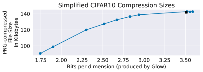
Figure S2: Simplified CIFAR10 images result in smaller storage space when converted into PNG files. Plotted are the average PNG file sizes of the simplified images after joint simplification and classification training (see Section 3), against $\mathrm{bpd}$ values produced by Glow, the generative model. Runs with different simplification loss weight $\lambda_{\textrm{sim}}$ lead to different average file sizes.

We want to validate that simplified images actually occupy less storage space. We save images in the PNG file format and calculate the file size. Figure S2 shows the average PNG file size of the simplified images obtained from our simplification framework. Concretely, we PNG-compress the images at the end of the joint simplification and classification training and then compute the average file size. Varying the simplification loss weight $\lambda_{\textrm{sim}}$ leads to different average $\mathrm{bpd}$ values and also different file sizes, with larger $\lambda_{\textrm{sim}}$ resulting in smaller file sizes.

Appendix S6 Learning Curves for Retraining

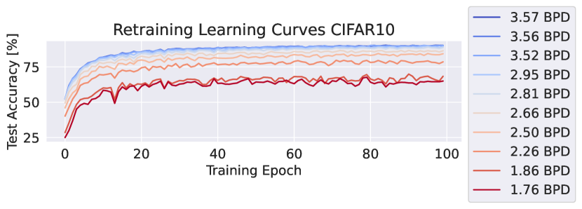
Figure S3: Learning curves for retraining on simplified images on CIFAR10.

Figure S3 shows learning curves during retraining on the simplified images on CIFAR10. There are no noticeable differences in training speed for more or less simplified images.

Appendix S7 Simplifier Baselines

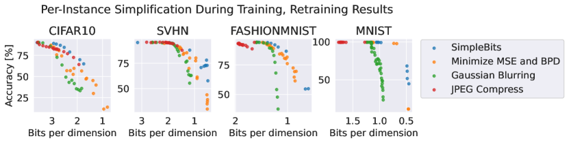
Figure S4: Comparison between SimpleBits and two simpler baselines: In the first one, the simplifier network is trained to simultaneously reduce $\mathrm{bpd}$ of the simplified image and the mean squared error between the simplified and the original image. In the second one, gaussian blurring is applied to the input images, different runs vary in the standard deviation used to create the gaussian blurring kernel. In the third one, we use JPEG compression with varying quality levels. Tradeoff curves are worse for the baselines than for SimpleBits .

We implemented three simpler baselines to check whether the losses used in SimpleBits during training help retain task-relevant information. In the first baseline, we train the simplifier to simultaneously reduce $\mathrm{bpd}$ of the simplified image and the mean squared error between the simplified and the original image. Afterwards we train the classifier on the simplified images and evaluate on the original images the same way as during retraining of SimpleBits. In the second baseline, we blur the original images with a gaussian kernel, which also reduces their bpd. We vary the sigma/standard deviation for the gaussian kernel to trade off smoothness and task-informativeness. In the third baseline, we use lossy JPEG compression with varying quality levels. As in SimpleBits and the other baselines, we estimate the bits per dimension of the lossy-JPEG-compressed images through our pretrained Glow network for a fair comparison. The gaussian blurring and JPEG compression each replace the simplifier, so these are fixed simplifier baselines without training a simplifier. While these three baselines also retain some task-relevant information allowing the classifier to retain above-chance accuracies (see Figure S4), the tradeoff between $\mathrm{bpd}$ and accuracy is worse than for SimpleBits. This shows the losses used in SimpleBits help retain more task-relevant information compared to these baselines.

Appendix S8 More Images Simplified During Training

We show a larger number of images that were simplified on CIFAR10 during training with the largest simplification loss weight $\lambda_{\textrm{sim}}=2.0$ in Figures S5, S6 and S7.

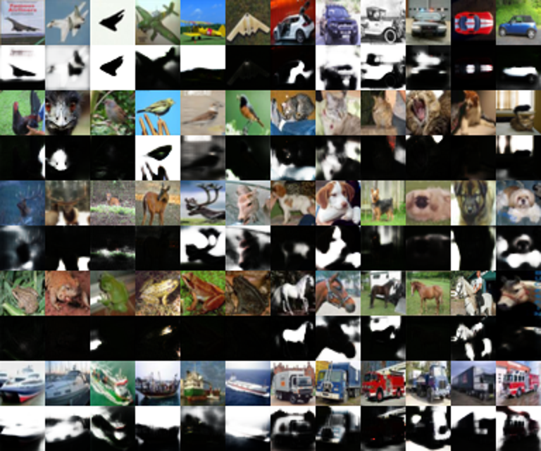
Figure S5: Uncurated set of simplified images with $\lambda_{\mathrm{sim}}=2.0$, 6 per class. Rows alternate between original and simplified images.

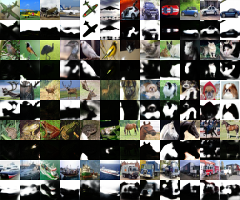
Figure S6: Uncurated set of correctly predicted simplified images with $\lambda_{\mathrm{sim}}=2.0$, 6 per class. Rows alternate between original and simplified images.

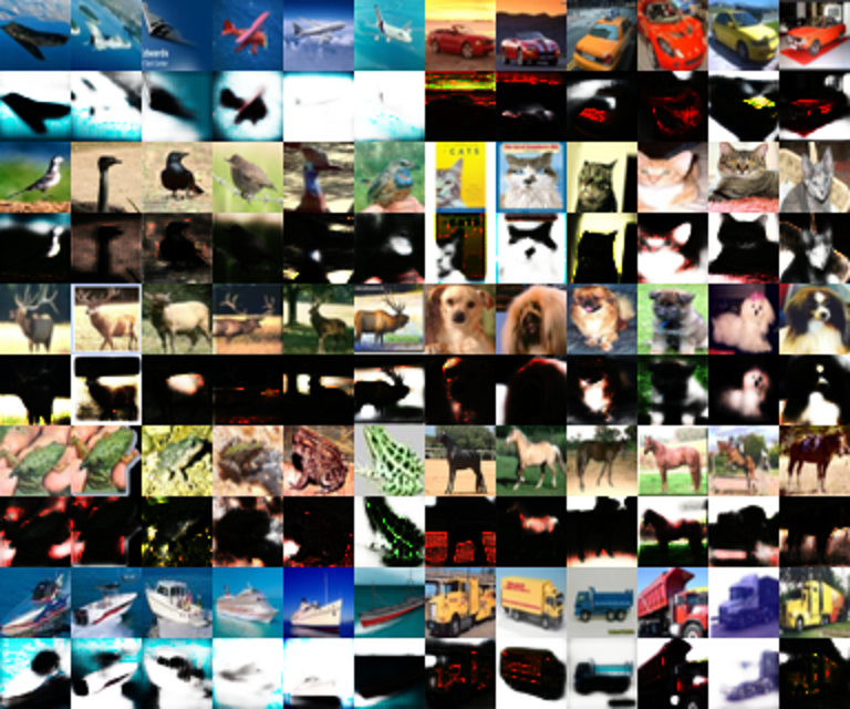
Figure S7: Correctly predicted simplified images with strongest color with $\lambda_{\mathrm{sim}}=2.0$, 6 per class.

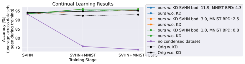
Figure S8: Continual Learning Results without Condensed Dataset (regular sequential training). Conventions as in Figure S9. Accuracies substantially worse without any condensed dataset.

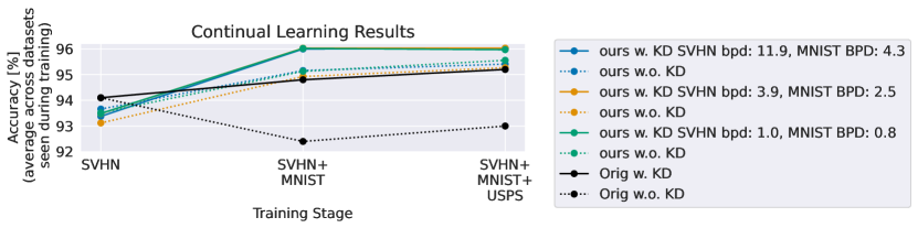
Figure S9: Continual Learning Results. Results for first training on SVHN, then MNIST and then USPS for condensed datasets with varying bits per dimension. Solid lines are with and dashed lines without knowledge distillation. Note that continual learning accuracies remain similar also for substantially reduced bits per dimension. Ablations show that accuracies degrade without any condensed dataset, see supplementary.

Appendix S9 Potentially spurious features uncovered by SimpleBits

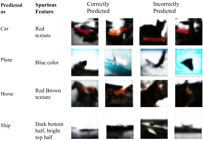
Figure S10: Selected simplified images that highlight potentially spurious features. Two leftmost images are correctly predicted, two rightmost images are incorrectly predicted.

SimpleBits may have the potential to reveal spurious correlations present in the dataset. We show some simplified images that reveal potentially spurious features in Figure S10. These observations can be used as a starting point to further investigate whether these features also affect regularly trained classifiers.

Appendix S10 More condensed datasets

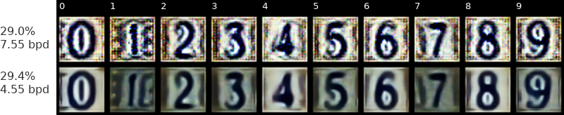
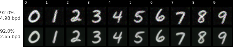
Figure S11: Dataset condensation results with varying simplification loss weight. Top: Individual dots represent accuracies for setting with different simplification loss weights. Accuracies can be retained even with substantially reduced bits per dimension. For 1 image per class, arrows highlight the settings that are visualized below. Below: Condensed datasets with varying simplification loss weight. Per dataset, showing condensed datasets with high (top row) and low (bottom row) bits per dimension. Lower bits per dimension datasets are visually simpler and smoother while mostly retaining accuracies.

We also show condensed datasets for MNIST and SVHN (Figure S11), some interesting condensed datasets that resulted when we varied the architecture (Figure S12) or the condensation loss (from gradient matching to either negative gradient product or single-training-step unrolling, Figure S13).

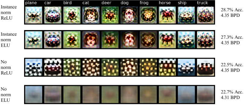
Figure S12: Dataset condensation on CIFAR10 with varying architecture.

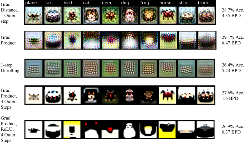
Figure S13: Dataset condensation on CIFAR10 with varying condensation loss and varying outer loop steps, i.e. how many steps the classifier is trained at each training epoch (default 1 in the 1 image per class setting), after each step the condensation loss is again optimized.

Appendix S11 Evaluation of Condensed Datasets for Continual Learning

We also evaluate the simplified condensed datasets in a continual learning setting, following (Zhao & Bilen, 2021). In this task-incremental continual learning setting, the model is trained on different classification datasets sequentially. When training on a new dataset, the model is additionally trained on the condensed versions of the previous datasets.

The continual learning experiment reproduces the setting from (Zhao & Bilen, 2021) to first train on SVHN, then on MNIST and finally on USPS (Hull, 1994), using the average accuracy across all three datasets of the classifier at the end of training as the final accuracy (see (Zhao & Bilen, 2021) for details).

We created a simpler and faster continual training pipeline that achieves comparable results to Zhao & Bilen (2021). First, we train 3 times for 50 epochs on SVHN, with a cosine annealing learning rate schedule (Loshchilov & Hutter, 2017) that is restarted at each time with $lr=0.1$. Then for each MNIST and USPS, we train one cosine annealing cycle of 50 epochs for $lr=0.1$.

We first verified that we can reproduce the prior continual learning results with our simpler training pipeline and find that our training pipeline indeed even slightly outperforms the reported final results (96.0% vs. 95.2% with, and 95.4% vs 93.0% without knowledge distillation) despite slightly inferior performance in the first training stage (before any continual learning, 93.6% vs 94.1%), see following subsection. When using different SVHN and MNIST condensed datasets, we find that we can retain the original continual learning accuracies even with condensed datasets with substantially less ($\sim$9x less) bits per dimension (see Fig.S9).

S11.1 Without Condensed Dataset

Our training pipeline still exhibits forgetting when not using any condensed datasets of previously trained-on datasets. As Figure S8 shows, the accuracies are far lower than with just regular sequential training. We performed this ablation to ensure forgetting still occurs in our training pipeline.

Appendix S12 More images Simplified After Training

We show further examples of post-hoc-simplified images for misclassified original images in Figure S14. We also show the output of SimpleBits when applied to the control images of Figure 8 in Figure S15 and a comparison to saliency-based methods in Figure S16. We also show an uncurated set of incorrectly predicted and correctly predicted images in Figures S17 and S18.

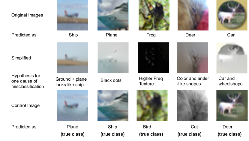
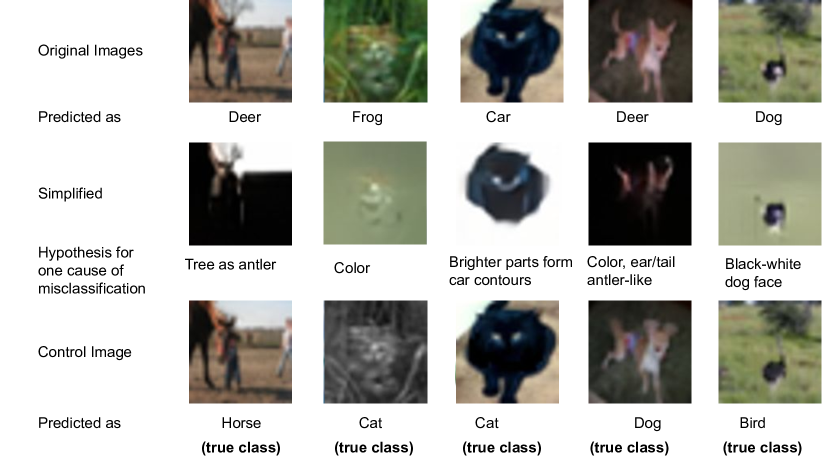
Figure S14: Further examples of post-hoc simplifications of originally misclassified images.

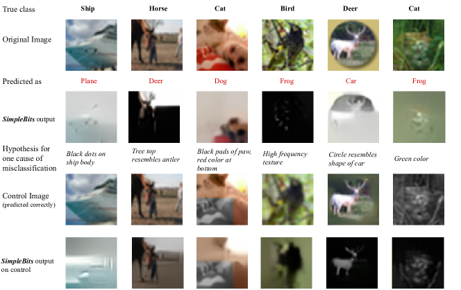
Figure S15: Post-hoc simplifications of control images.

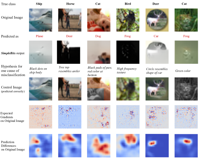
Figure S16: Post-hoc simplifications of misclassified CIFAR-10 examples and saliency maps. In this figure, we also show color-coded saliency maps for expected gradients (Erion et al., 2021) and prediction difference (Zintgraf et al., 2017) for comparison (red: evidence for and blue: evidence against the predicted class). SimpleBits reveals more information than saliency methods.

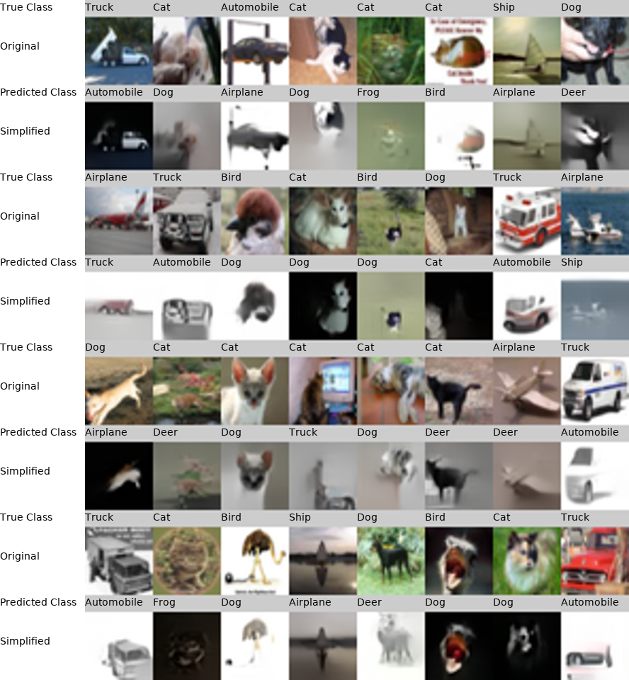
Figure S17: Uncurated post-hoc simplifications of incorrectly predicted images.

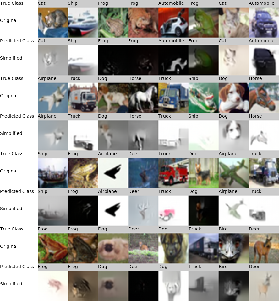
Figure S18: Uncurated post-hoc simplifications of correctly predicted images.

References

- Agarwal et al. (2021) Agarwal, C., D’souza, D., and Hooker, S. Estimating example difficulty using variance of gradients, 2021.
- Banerjee et al. (2021a) Banerjee, I., Bhimireddy, A. R., Burns, J. L., Celi, L. A., Chen, L., Correa, R., Dullerud, N., Ghassemi, M., Huang, S., Kuo, P., Lungren, M. P., Palmer, L. J., Price, B. J., Purkayastha, S., Pyrros, A., Oakden-Rayner, L., Okechukwu, C., Seyyed-Kalantari, L., Trivedi, H., Wang, R., Zaiman, Z., Zhang, H., and Gichoya, J. W. Reading race: AI recognises patient’s racial identity in medical images. CoRR, abs/2107.10356, 2021a. URL https://arxiv.org/abs/2107.10356.
- Banerjee et al. (2021b) Banerjee, I., Bhimireddy, A. R., Burns, J. L., Celi, L. A., Chen, L.-C., Correa, R., Dullerud, N., Ghassemi, M., Huang, S.-C., Kuo, P.-C., Lungren, M. P., Palmer, L., Price, B. J., Purkayastha, S., Pyrros, A., Oakden-Rayner, L., Okechukwu, C., Seyyed-Kalantari, L., Trivedi, H., Wang, R., Zaiman, Z., Zhang, H., and Gichoya, J. W. Reading race: Ai recognises patient’s racial identity in medical images, 2021b.
- Bastings et al. (2021) Bastings, J., Ebert, S., Zablotskaia, P., Sandholm, A., and Filippova, K. "will you find these shortcuts?" a protocol for evaluating the faithfulness of input salience methods for text classification, 2021.
- Bellemare et al. (2003) Bellemare, F., Jeanneret, A., and Couture, J. Sex differences in thoracic dimensions and configuration. American journal of respiratory and critical care medicine, 168(3):305–312, 2003.
- Brock et al. (2021) Brock, A., De, S., Smith, S. L., and Simonyan, K. High-performance large-scale image recognition without normalization. In Meila, M. and Zhang, T. (eds.), Proceedings of the 38th International Conference on Machine Learning, ICML 2021, 18-24 July 2021, Virtual Event, volume 139 of Proceedings of Machine Learning Research, pp. 1059–1071. PMLR, 2021. URL http://proceedings.mlr.press/v139/brock21a.html.
- Dombrowski et al. (2021) Dombrowski, A.-K., Gerken, J. E., and Kessel, P. Diffeomorphic explanations with normalizing flows. In ICML Workshop on Invertible Neural Networks, Normalizing Flows, and Explicit Likelihood Models, 2021. URL https://openreview.net/forum?id=ZBR9EpEl6G4.
- D’souza et al. (2021) D’souza, D., Nussbaum, Z., Agarwal, C., and Hooker, S. A tale of two long tails, 2021.
- Dubois et al. (2021) Dubois, Y., Bloem-Reddy, B., Ullrich, K., and Maddison, C. J. Lossy compression for lossless prediction. CoRR, abs/2106.10800, 2021. URL https://arxiv.org/abs/2106.10800.
- Erion et al. (2021) Erion, G., Janizek, J. D., Sturmfels, P., Lundberg, S. M., and Lee, S.-I. Improving performance of deep learning models with axiomatic attribution priors and expected gradients. Nature Machine Intelligence, pp. 1–12, 2021.
- Finn et al. (2017) Finn, C., Abbeel, P., and Levine, S. Model-agnostic meta-learning for fast adaptation of deep networks. In Precup, D. and Teh, Y. W. (eds.), Proceedings of the 34th International Conference on Machine Learning, ICML 2017, Sydney, NSW, Australia, 6-11 August 2017, volume 70 of Proceedings of Machine Learning Research, pp. 1126–1135. PMLR, 2017. URL http://proceedings.mlr.press/v70/finn17a.html.
- Geirhos et al. (2020) Geirhos, R., Jacobsen, J.-H., Michaelis, C., Zemel, R., Brendel, W., Bethge, M., and Wichmann, F. A. Shortcut learning in deep neural networks. Nature Machine Intelligence, 2(11):665–673, 2020.
- Goyal et al. (2019) Goyal, Y., Wu, Z., Ernst, J., Batra, D., Parikh, D., and Lee, S. Counterfactual visual explanations. In Chaudhuri, K. and Salakhutdinov, R. (eds.), Proceedings of the 36th International Conference on Machine Learning, ICML 2019, 9-15 June 2019, Long Beach, California, USA, volume 97 of Proceedings of Machine Learning Research, pp. 2376–2384. PMLR, 2019. URL http://proceedings.mlr.press/v97/goyal19a.html.
- Havtorn et al. (2021) Havtorn, J. D., Frellsen, J., Hauberg, S., and Maaløe, L. Hierarchical vaes know what they don’t know. In Meila, M. and Zhang, T. (eds.), Proceedings of the 38th International Conference on Machine Learning, ICML 2021, 18-24 July 2021, Virtual Event, volume 139 of Proceedings of Machine Learning Research, pp. 4117–4128. PMLR, 2021. URL http://proceedings.mlr.press/v139/havtorn21a.html.
- Hinton & van Camp (1993) Hinton, G. E. and van Camp, D. Keeping the neural networks simple by minimizing the description length of the weights. In Pitt, L. (ed.), Proceedings of the Sixth Annual ACM Conference on Computational Learning Theory, COLT 1993, Santa Cruz, CA, USA, July 26-28, 1993, pp. 5–13. ACM, 1993. doi: 10.1145/168304.168306. URL https://doi.org/10.1145/168304.168306.
- Hooker et al. (2019) Hooker, S., Erhan, D., Kindermans, P.-J., and Kim, B. A benchmark for interpretability methods in deep neural networks. In Wallach, H., Larochelle, H., Beygelzimer, A., dÁlché-Buc, F., Fox, E., and Garnett, R. (eds.), Advances in Neural Information Processing Systems, volume 32. Curran Associates, Inc., 2019. URL https://proceedings.neurips.cc/paper/2019/file/fe4b8556000d0f0cae99daa5c5c5a410-Paper.pdf.
- Huang et al. (2016) Huang, G., Sun, Y., Liu, Z., Sedra, D., and Weinberger, K. Q. Deep networks with stochastic depth. In Leibe, B., Matas, J., Sebe, N., and Welling, M. (eds.), Computer Vision - ECCV 2016 - 14th European Conference, Amsterdam, The Netherlands, October 11-14, 2016, Proceedings, Part IV, volume 9908 of Lecture Notes in Computer Science, pp. 646–661. Springer, 2016. doi: 10.1007/978-3-319-46493-0\_39. URL https://doi.org/10.1007/978-3-319-46493-0_39.
- Hull (1994) Hull, J. J. A database for handwritten text recognition research. IEEE Trans. Pattern Anal. Mach. Intell., 16(5):550–554, 1994. doi: 10.1109/34.291440. URL https://doi.org/10.1109/34.291440.
- Hvilshøj et al. (2021) Hvilshøj, F., Iosifidis, A., and Assent, I. ECINN: efficient counterfactuals from invertible neural networks. CoRR, abs/2103.13701, 2021. URL https://arxiv.org/abs/2103.13701.
- Jany & Welte (2019) Jany, B. and Welte, T. Pleural effusion in adults—etiology, diagnosis, and treatment. Deutsches Ärzteblatt International, 116(21):377, 2019.
- Johnson et al. (2019a) Johnson, A. E., Pollard, T. J., Berkowitz, S. J., Greenbaum, N. R., Lungren, M. P., Deng, C.-y., Mark, R. G., and Horng, S. Mimic-cxr, a de-identified publicly available database of chest radiographs with free-text reports. Scientific data, 6(1):1–8, 2019a.
- Johnson et al. (2019b) Johnson, A. E., Pollard, T. J., Greenbaum, N. R., Lungren, M. P., Deng, C.-y., Peng, Y., Lu, Z., Mark, R. G., Berkowitz, S. J., and Horng, S. Mimic-cxr-jpg, a large publicly available database of labeled chest radiographs. arXiv preprint arXiv:1901.07042, 2019b.
- Kingma & Ba (2015) Kingma, D. P. and Ba, J. Adam: A method for stochastic optimization. In Bengio, Y. and LeCun, Y. (eds.), 3rd International Conference on Learning Representations, ICLR 2015, San Diego, CA, USA, May 7-9, 2015, Conference Track Proceedings, 2015. URL http://arxiv.org/abs/1412.6980.
- Kingma & Dhariwal (2018) Kingma, D. P. and Dhariwal, P. Glow: Generative flow with invertible 1x1 convolutions. In Bengio, S., Wallach, H., Larochelle, H., Grauman, K., Cesa-Bianchi, N., and Garnett, R. (eds.), Advances in Neural Information Processing Systems (NeuRIPs), pp. 10215–10224, 2018.
- Kirichenko et al. (2020) Kirichenko, P., Izmailov, P., and Wilson, A. G. Why normalizing flows fail to detect out-of-distribution data. In Larochelle, H., Ranzato, M., Hadsell, R., Balcan, M., and Lin, H. (eds.), Advances in Neural Information Processing Systems 33: Annual Conference on Neural Information Processing Systems 2020, NeurIPS 2020, December 6-12, 2020, virtual, 2020. URL https://proceedings.neurips.cc/paper/2020/hash/ecb9fe2fbb99c31f567e9823e884dbec-Abstract.html.
- Krizhevsky (2009) Krizhevsky, A. Learning multiple layers of features from tiny images. Technical report, 2009.
- LeCun & Cortes (2010) LeCun, Y. and Cortes, C. MNIST handwritten digit database. 2010. URL http://yann.lecun.com/exdb/mnist/.
- Loshchilov & Hutter (2017) Loshchilov, I. and Hutter, F. SGDR: stochastic gradient descent with warm restarts. In 5th International Conference on Learning Representations, ICLR 2017, Toulon, France, April 24-26, 2017, Conference Track Proceedings. OpenReview.net, 2017. URL https://openreview.net/forum?id=Skq89Scxx.
- Loshchilov & Hutter (2019) Loshchilov, I. and Hutter, F. Decoupled weight decay regularization. In 7th International Conference on Learning Representations, ICLR 2019, New Orleans, LA, USA, May 6-9, 2019. OpenReview.net, 2019. URL https://openreview.net/forum?id=Bkg6RiCqY7.
- Maclaurin et al. (2015) Maclaurin, D., Duvenaud, D., and Adams, R. Gradient-based hyperparameter optimization through reversible learning. In Bach, F. and Blei, D. (eds.), Proceedings of the 32nd International Conference on Machine Learning, volume 37 of Proceedings of Machine Learning Research, pp. 2113–2122, Lille, France, 07–09 Jul 2015. PMLR. URL https://proceedings.mlr.press/v37/maclaurin15.html.
- Madsen et al. (2021) Madsen, A., Meade, N., Adlakha, V., and Reddy, S. Evaluating the faithfulness of importance measures in nlp by recursively masking allegedly important tokens and retraining, 2021.
- Makino et al. (2020) Makino, T., Jastrzebski, S., Oleszkiewicz, W., Chacko, C., Ehrenpreis, R., Samreen, N., Chhor, C., Kim, E., Lee, J., Pysarenko, K., et al. Differences between human and machine perception in medical diagnosis. arXiv preprint arXiv:2011.14036, 2020.
- Montavon et al. (2018) Montavon, G., Samek, W., and Müller, K.-R. Methods for interpreting and understanding deep neural networks. Digital Signal Processing, 73:1–15, 2018. ISSN 1051-2004. doi: https://doi.org/10.1016/j.dsp.2017.10.011. URL https://www.sciencedirect.com/science/article/pii/S1051200417302385.
- Netzer et al. (2011) Netzer, Y., Wang, T., Coates, A., Bissacco, A., Wu, B., and Ng, A. Y. Reading digits in natural images with unsupervised feature learning. In NIPS Workshop on Deep Learning and Unsupervised Feature Learning, 2011.
- Nguyen et al. (2021) Nguyen, T., Novak, R., Xiao, L., and Lee, J. Dataset distillation with infinitely wide convolutional networks. CoRR, abs/2107.13034, 2021. URL https://arxiv.org/abs/2107.13034.
- Pham et al. (2021) Pham, H., Dai, Z., Xie, Q., and Le, Q. V. Meta pseudo labels. In IEEE Conference on Computer Vision and Pattern Recognition, CVPR 2021, virtual, June 19-25, 2021, pp. 11557–11568. Computer Vision Foundation / IEEE, 2021. URL https://openaccess.thecvf.com/content/CVPR2021/html/Pham_Meta_Pseudo_Labels_CVPR_2021_paper.html.
- Raasch et al. (1982) Raasch, B., Carsky, E., Lane, E., O’Callaghan, J., and Heitzman, E. Pleural effusion: explanation of some typical appearances. American Journal of Roentgenology, 139(5):899–904, 1982.
- Radford et al. (2021) Radford, A., Kim, J. W., Hallacy, C., Ramesh, A., Goh, G., Agarwal, S., Sastry, G., Askell, A., Mishkin, P., Clark, J., et al. Learning transferable visual models from natural language supervision. arXiv preprint arXiv:2103.00020, 2021.
- Raghu et al. (2021) Raghu, A., Raghu, M., Kornblith, S., Duvenaud, D., and Hinton, G. E. Teaching with commentaries. In 9th International Conference on Learning Representations, ICLR 2021, Virtual Event, Austria, May 3-7, 2021. OpenReview.net, 2021. URL https://openreview.net/forum?id=4RbdgBh9gE.
- Raghu & Schmidt (2020) Raghu, M. and Schmidt, E. A survey of deep learning for scientific discovery. arXiv preprint arXiv:2003.11755, 2020.
- Ronneberger et al. (2015) Ronneberger, O., Fischer, P., and Brox, T. U-net: Convolutional networks for biomedical image segmentation. In Navab, N., Hornegger, J., III, W. M. W., and Frangi, A. F. (eds.), Medical Image Computing and Computer-Assisted Intervention - MICCAI 2015 - 18th International Conference Munich, Germany, October 5 - 9, 2015, Proceedings, Part III, volume 9351 of Lecture Notes in Computer Science, pp. 234–241. Springer, 2015. doi: 10.1007/978-3-319-24574-4\_28. URL https://doi.org/10.1007/978-3-319-24574-4_28.
- Schirrmeister et al. (2020) Schirrmeister, R., Zhou, Y., Ball, T., and Zhang, D. Understanding anomaly detection with deep invertible networks through hierarchies of distributions and features. In Larochelle, H., Ranzato, M., Hadsell, R., Balcan, M., and Lin, H. (eds.), Advances in Neural Information Processing Systems 33: Annual Conference on Neural Information Processing Systems 2020, NeurIPS 2020, December 6-12, 2020, virtual, 2020. URL https://proceedings.neurips.cc/paper/2020/hash/f106b7f99d2cb30c3db1c3cc0fde9ccb-Abstract.html.
- Serrà et al. (2020) Serrà, J., Álvarez, D., Gómez, V., Slizovskaia, O., Núñez, J. F., and Luque, J. Input complexity and out-of-distribution detection with likelihood-based generative models. In 8th International Conference on Learning Representations, ICLR 2020, Addis Ababa, Ethiopia, April 26-30, 2020. OpenReview.net, 2020. URL https://openreview.net/forum?id=SyxIWpVYvr.
- Shannon (1948) Shannon, C. E. A mathematical theory of communication. The Bell System Technical Journal, 27(3):379–423, July 1948.
- Singla et al. (2020) Singla, S., Pollack, B., Chen, J., and Batmanghelich, K. Explanation by progressive exaggeration. In 8th International Conference on Learning Representations, ICLR 2020, Addis Ababa, Ethiopia, April 26-30, 2020. OpenReview.net, 2020. URL https://openreview.net/forum?id=H1xFWgrFPS.
- Torralba et al. (2008) Torralba, A., Fergus, R., and Freeman, W. T. 80 million tiny images: A large data set for nonparametric object and scene recognition. IEEE Transactions on Pattern Analysis and Machine Intelligence, 30(11):1958–1970, 2008.
- Wang et al. (2018) Wang, T., Zhu, J., Torralba, A., and Efros, A. A. Dataset distillation. CoRR, abs/1811.10959, 2018. URL http://arxiv.org/abs/1811.10959.
- Xiao et al. (2017) Xiao, H., Rasul, K., and Vollgraf, R. Fashion-mnist: a novel image dataset for benchmarking machine learning algorithms, 2017.
- Zagoruyko & Komodakis (2016) Zagoruyko, S. and Komodakis, N. Wide residual networks. In Wilson, R. C., Hancock, E. R., and Smith, W. A. P. (eds.), Proceedings of the British Machine Vision Conference 2016, BMVC 2016, York, UK, September 19-22, 2016. BMVA Press, 2016. URL http://www.bmva.org/bmvc/2016/papers/paper087/index.html.
- Zhao & Bilen (2021) Zhao, B. and Bilen, H. Dataset condensation with differentiable siamese augmentation. In Meila, M. and Zhang, T. (eds.), Proceedings of the 38th International Conference on Machine Learning, ICML 2021, 18-24 July 2021, Virtual Event, volume 139 of Proceedings of Machine Learning Research, pp. 12674–12685. PMLR, 2021. URL http://proceedings.mlr.press/v139/zhao21a.html.
- Zhao et al. (2021) Zhao, B., Mopuri, K. R., and Bilen, H. Dataset condensation with gradient matching. In 9th International Conference on Learning Representations, ICLR 2021, Virtual Event, Austria, May 3-7, 2021. OpenReview.net, 2021. URL https://openreview.net/forum?id=mSAKhLYLSsl.
- Zintgraf et al. (2017) Zintgraf, L. M., Cohen, T. S., Adel, T., and Welling, M. Visualizing deep neural network decisions: Prediction difference analysis. In 5th International Conference on Learning Representations, ICLR 2017, Toulon, France, April 24-26, 2017, Conference Track Proceedings. OpenReview.net, 2017. URL https://openreview.net/forum?id=BJ5UeU9xx.