Range separation of the Coulomb hole^†‡

Abstract

A range-separation of the Coulomb hole into two components, one of them being predominant at long interelectronic separations ($h_{\text{c}_{I}}$) and the other at short distances ($h_{\text{c}_{II}}$), is exhaustively analyzed throughout various examples that put forward the most relevant features of this approach and how they can be used to develop efficient ways to capture electron correlation. We show that $h_{\text{c}_{I}}$, which only depends on the first-order reduced density matrix, can be used to identify molecules with a predominant nondynamic correlation regime and differentiate between two types of nondynamic correlation, types A and B. Through the asymptotic properties of the hole components, we explain how $h_{\text{c}_{I}}$ can retrieve the long-range part of electron correlation. We perform an exhaustive analysis of the hydrogen molecule in a minimal basis set, dissecting the hole contributions into spin components. We also analyze the simplest molecule presenting a dispersion interaction and how $h_{\text{c}_{II}}$ helps identify it. The study of several atoms in different spin states reveals that the Coulomb hole components distinguish correlation regimes that are not apparent from the entire hole. The results of this work hold the promise to aid in developing new electronic structure methods that efficiently capture electron correlation.

1 Introduction

In computational chemistry, the difference between the exact nonrelativistic electronic energy and the restricted Hartree–Fock (RHF) one is known as correlation energy.¹ Even though the uncorrelated, self-consistent field (SCF) HF energy usually represents more than 98% of the total energy, the remaining is crucial to describe the chemistry of atoms and molecules (dissociation energies, reaction enthalpies, etcetera). ^{2, 3} The description of a quantum system with the HF method lacks electron correlation, i.e., a correct account of the correlated motion of the electrons. This conundrum is generally known as the many-body problem, and it is one of the main challenges in this field.^{2, 3} The study of electron correlation per se goes hand in hand with developing efficient electronic structure methods.^{4, 5, 6, 7, 8, 9, 10, 11, 12, 13, 14, 15, 16, 17, 18, 19, 20, 21, 22}

Many types of electron correlation exist, nondynamic (or static) ^{23, 24, 2} and dynamic ^{24, 2} being the most regularly used because electronic structure methods are usually classified according to their ability to retrieve them. Dynamic correlation is universally present in systems with at least two electrons, as it describes the motion of charged particles avoiding each other due to the electronic repulsion. Hence, this type of correlation increases with the number of electrons. A reference single-determinant picture along with a large number of low-contributing configurations is usually sufficient to portray this contribution. It is thus natural that the electron density displays very small differences with respect to the reference HF density.^{14, 15, 22} Due to its nature, dynamic correlation affects electrons that are close to each other (short-ranged), but it is also responsible for long-range dispersion forces. ²⁵ Configuration interactions or coupled cluster with single and double excitations (CISD or CCSD), ^{26, 27} Møller-Plesset second-order perturbation theory (MP2) ²⁸ and density functional approximations (DFAs) ^{29, 6} are methods that retrieve a large amount of dynamic correlation. On the other hand, nondynamic correlation is not universal and emerges in the presence of partially-occupied (near-)degenerate orbitals. It is characteristic of bond stretching, polyradical structures, entanglement, and high symmetries. The correct description of nondynamic correlation requires a wavefunction that mixes other largely-contributing configurations besides the HF ground-state one. ³⁰ Nondynamic correlation induces considerable changes in the electron density caused by the mix of highly-contributing configurations in the CI vector. ^{14, 15, 16, 20, 21, 22} Complete active space SCF (CASSCF), ³¹ density matrix renormalization group (DMRG), ³² and multi-configurational SCF (MCSCF) ^{33, 34} are methods that can retrieve a fair amount of nondynamic correlation. As we shall confirm later, nondynamic correlation is important both at short and long range.

Systems presenting dynamic and nondynamic correlation have become one of the greatest challenges in modern electronic structure methods. The ability to simultaneously tackle both types of correlation is present in very few electronic structure methods, such as the complete active space with second-order perturbation theory (CASPT2), ^{35, 36} multireference configuration interactions (MRCI) ^{37, 38} or, most recently, the adiabatic-connection MCSCF (AC-MCSCF) ³⁹, $\Delta$NO, ⁴⁰ and GNOF. ⁴¹ Nevertheless, these methods are far from exact and their computational cost represents a big drawback. Latterly, an interest in hybrid schemes such as range-separated methods ^{42, 43} has surged to confront the exposed problem. These methods aim to recover both correlation types by treating short- and long-range interactions with two different methodologies, according to their ability to recover one of the correlation components. ^{43, 44, 45, 46, 47, 48, 49, 42, 50, 51, 52} Although range-separation hybrid schemes provide a splitting of the pair density and the interelectronic coordinate, the separation is not custom-built for the correlation type present in the system.

Some studies have put forward measures for quantifying dynamic and nondynamic correlation, ^{8, 9, 10, 11, 12, 13, 14, 15, 16, 17, 18, 19} some of which are based on the correlation energy. ^{14, 15, 16, 17, 18, 19} As reported by Coleman, ⁵³ the use of electron-pair distribution functions to study electron correlation must lead to an understanding of both short- and long-range interelectronic interactions. In line with the former statement, we have recently proposed a general decomposition scheme to separate the correlation part of the pair density into two components that permit the identification of systems with prevalent dynamic or nondynamic correlation. ^{20, 21, 22} From this scheme, scalar ²⁰ and local ²¹ measures of dynamic and nondynamic correlation have been developed. Finally, a range-separation of the Coulomb hole has been introduced, providing the dominance of one component at long ranges (c_I) and the other one (c_II) at short ranges. c_I —which only requires the first-order reduced density matrix (1-RDM)— has been shown to reflect nondynamic correlation, whereas c_II includes both correlation types. ²²

In the present work, the range separation of the Coulomb hole is exhaustively analyzed throughout various examples that put forward the most relevant features of this approach and how they can be used to develop efficient ways to capture electron correlation. First of all, we introduce the range-separation of the Coulomb hole and its rationalization. Through the asymptotic properties of the hole parts, we explain how the component based on the first-order reduced density matrix can retrieve the long-range part of the correlated pair density. Second, we perform an exhaustive analysis of the hydrogen molecule in a minimal basis set, dissecting the hole contributions into spin components. Third, we analyze the simplest molecule presenting a dispersion interaction and how one of the Coulomb hole components helps identify it. This dispersion signature is also present in the remaining molecules of the manuscript, highlighting its universal character. Afterward, we analyze the Coulomb holes of several atoms in different spin states, finding that the Coulomb hole components distinguish correlation regimes that are not apparent from the entire hole. Finally, we analyze the two types of nondynamic correlation, types A and B,¹¹ and show that the Coulomb hole’s first component can capture them.

The results of this work hold the promise to aid in developing new electronic structure methods that efficiently capture electron correlation. In particular, the models of the $c_{II}$ component can be straightforwardly used in the reduced density matrix functional theory,^{54, 55, 56, 57, 58} although they are not limited to this theory.

2 Methodology

The pair density of an $N$-electron system described by the $\Psi(\boldsymbol{1},\dots,\boldsymbol{N})$ wavefunction is

$$\rho_{2}(\boldsymbol{1},\boldsymbol{2})=N(N-1)\int\text{d}_{\boldsymbol{3}}\dots\text{d}_{\boldsymbol{N}}|\Psi(\boldsymbol{1},\dots,\boldsymbol{N})|^{2},$$ (1)

where we have assumed McWeeny’s normalization, ⁵⁹ which accounts for the number of electron pairs in the system, and the variables $\left(\boldsymbol{1},\boldsymbol{2},\ldots\right)$ refer to both space and spin coordinates, $\boldsymbol{1}\equiv\vec{r}_{1},\sigma_{1}$. The pair density contains information about the probability of finding electron $1$ at the position and spin $\boldsymbol{1}$ and electron $2$ at the position and spin $\boldsymbol{2}$ when the position of the remaining of $N-2$ electrons is averaged over the whole space. The analysis of the pair density is arduous since it depends on six space and two spin variables. Conversely, the radial intracule density is a reduced form of the pair density that only depends on the interelectronic distance or range separation, $s$, and still retains the necessary information to calculate the electronic repulsion energy,

$$V_{ee}=\frac{1}{2}\int\text{d}s\frac{I(\rho_{2},s)}{s},$$ (2)

being

$$I(\rho_{2},s)=\int\text{d}_{\boldsymbol{1}}\text{d}_{\boldsymbol{2}}\,\rho_{2}(\boldsymbol{1},\boldsymbol{2})\delta(s-r_{12}),$$ (3)

where $r_{12}$ is the Euclidean distance between electrons 1 and 2, and $\delta(s-r_{12})$ is the Dirac delta. Eq 3 is the radial intracule density and it corresponds to the probability distribution of interelectronic distances $s$ between two electrons. It provides information about the electron-pair relative motion within atoms and molecules, being also a valid quantity to interpret the electronic structure of atoms and chemical bonding.^{60, 61, 62, 63, 64} This distribution can also be obtained experimentally from X-ray scattering cross-sections. ^{65, 66, 67, 68}

After Löwdin’s definition of correlation energy, ¹ Coulson defined the correlated pair density as the difference between the exact and the HF pair densities, ⁶⁹

$$\Delta\rho_{2}^{\text{c}}(\boldsymbol{1},\boldsymbol{2})=\rho_{2}(\boldsymbol{1},\boldsymbol{2})-\rho_{2}^{\text{HF}}(\boldsymbol{1},\boldsymbol{2}).$$ (4)

The correlated pair density intracule $\Delta\rho_{2}^{\text{c}}(\boldsymbol{1},\boldsymbol{2})$ is known as Coulson’s Coulomb hole: ^{70, 71, 72}

$$h_{\text{c}}\left(s\right)=I\left(\Delta\rho_{2}^{\text{c}},s\right)=I\left(\rho_{2},s\right)-I\left(\rho_{2}^{\text{HF}},s\right).$$ (5)

The Coulomb hole is thus a probability density difference that reflects the effect of switching from the mean-field HF approximation, which underestimates the electronic repulsion, to a correlated framework. As a result, the average interelectronic distance increases from HF to the exact description, $\langle s\rangle_{\text{HF}}<\langle s\rangle$ ($\langle s\rangle=\int I(s)sds$); this effect is reflected by the negative values of the Coulomb hole at small values of $s$ and positives values at large $s$.

We have introduced elsewhere ^{20, 21, 22} a splitting of the correlated pair density, eq 4, using the single-determinant approximation to the pair density, ¹

$$\rho_{2}^{\text{SD}}\left(\rho_{1},\boldsymbol{1},\boldsymbol{2}\right)=\rho(\boldsymbol{1})\rho(\boldsymbol{2})-|\rho_{1}\left(\boldsymbol{1};\boldsymbol{2}\right)|^{2},$$ (6)

where $\rho_{1}\left(\boldsymbol{1};\boldsymbol{2}\right)$ is the first-order reduced density matrix (1-RDM),

$$\rho_{1}\left(\boldsymbol{1};\boldsymbol{1^{\prime}}\right)=\int\text{d}_{\boldsymbol{2}}\ldots\text{d}_{\boldsymbol{N}}\Psi\left(\boldsymbol{1},\boldsymbol{2},\ldots,\boldsymbol{N}\right)\Psi^{*}\left(\boldsymbol{1^{\prime}},\boldsymbol{2},\ldots,\boldsymbol{N}\right),$$ (7)

and its diagonal part, $\rho\left(\boldsymbol{1}\right)=\rho\left(\boldsymbol{1},\boldsymbol{1}\right)$, is the electron density. The SD ansatz, eq 6, takes advantage of the HF expression for the pair density but uses the actual 1-RDM to generate an approximation to the pair density. Obviously, it returns the HF pair density when the HF 1-RDM is used, i.e.,

$$\rho_{2}^{\text{HF}}\left(\boldsymbol{1},\boldsymbol{2}\right)=\rho_{2}^{\text{SD}}\left(\rho_{1}^{\text{HF}},\boldsymbol{1},\boldsymbol{2}\right).$$ (8)

The SD approximation includes neither short- ⁷³ nor long-range ⁷⁴ dynamic correlation, that is, it only considers nondynamic correlation. Even though it cannot be guaranteed that all nondynamic correlation in the system is accounted for, it is legitimate to claim that the SD pair density, eq 6, includes some extent of it. In fact, the SD approximation captures most long-range electron correlation effects and usually presents a minimal short-range contribution that arises from the relative degeneracy of its frontier orbitals (except for systems with type B nondynamic correlation,¹¹ vide infra). Unlike the HF pair density, the SD approximation is usually not $N$-representable by construction, i.e., this approximate pair density does not necessarily correspond to an $N$-particle fermionic wavefunction. The violation of the $N$-representability conditions may lead to spurious energies ⁷⁵ and affect density matrix properties as the trace, $\text{Tr}\left[\rho_{2}^{\text{SD}}\right]$, or the positivity of its eigenvalues, among others. ^{76, 77, 73, 78, 79, 80} Although it is not $N$-representable, $\rho_{2}^{\text{SD}}\left(\boldsymbol{1},\boldsymbol{2}\right)$ is used in this context as a mathematical approximation to seize long-range correlation. Indeed, we have used it to separate eq 4 into two correlation contributions, $\Delta\rho_{2}^{\text{c}_{\textit{I}}}$ and $\Delta\rho_{2}^{\text{c}_{\textit{II}}}$,²²

$$\Delta\rho_{2}^{\text{c}_{\textit{I}}}(\boldsymbol{1},\boldsymbol{2}) = \rho_{2}^{\text{SD}}\left(\rho_{1},\boldsymbol{1},\boldsymbol{2}\right)-\rho_{2}^{\text{SD}}\left(\rho_{1}^{\text{HF}},\boldsymbol{1},\boldsymbol{2}\right)$$ (9)

$$\Delta\rho_{2}^{\text{c}_{\textit{II}}}(\boldsymbol{1},\boldsymbol{2}) = \rho_{2}\left(\rho_{1},\boldsymbol{1},\boldsymbol{2}\right)-\rho_{2}^{\text{SD}}\left(\rho_{1},\boldsymbol{1},\boldsymbol{2}\right),$$ (10)

which, along with the HF pair density, recover the exact pair density:

$$\rho_{2}\left(\boldsymbol{1},\boldsymbol{2}\right)=\rho_{2}^{\text{HF}}\left(\boldsymbol{1},\boldsymbol{2}\right)+\Delta\rho_{2}^{\text{c}_{\textit{I}}}\left(\boldsymbol{1},\boldsymbol{2}\right)+\Delta\rho_{2}^{\text{c}_{\textit{II}}}\left(\boldsymbol{1},\boldsymbol{2}\right).$$ (11)

The partition of the pair density into the HF reference plus the $c_{I}$ component and the $c_{II}$ part is known as the Lieb partitioning of the pair density.^{81, 82, 83} $\Delta\rho_{2}^{\text{c}_{\textit{II}}}\left(\boldsymbol{1},\boldsymbol{2}\right)$ is also known as the cumulant of the density matrix and captures the correlation lacking in the 2-RDM.^{84, 85} $\Delta\rho_{2}^{\text{c}_{\textit{I}}}\left(\boldsymbol{1},\boldsymbol{2}\right)$ only depends on the actual 1-RDM and the HF one measures the dissimilarity between these two matrices. The electron density of systems with nondynamic correlation presents more considerable differences with respect to HF than the density of systems with dynamic correlation.¹⁵ Therefore, $\Delta\rho_{2}^{\text{c}_{\textit{I}}}\left(\boldsymbol{1},\boldsymbol{2}\right)$ can be regarded as a function measuring nondynamic correlation, whereas the information about dynamic correlation is expected to be fully contained in $\Delta\rho_{2}^{\text{c}_{\textit{II}}}\left(\boldsymbol{1},\boldsymbol{2}\right)$, which also includes nondynamic correlation to some extent.

A more explicit expression for eqs 9 and 10 can be cast:

$$\Delta\rho_{2}^{\text{c}_{\textit{I}}}\left(\boldsymbol{1},\boldsymbol{2}\right)=|\rho_{1}^{\text{HF}}\left(\boldsymbol{1};\boldsymbol{2}\right)|^{2}-|\rho_{1}\left(\boldsymbol{1};\boldsymbol{2}\right)|^{2}+\rho(\boldsymbol{1})\rho(\boldsymbol{2})-\rho^{\text{HF}}(\boldsymbol{1})\rho^{\text{HF}}(\boldsymbol{2})\hskip 17.07182pt$$ (12)

$$\Delta\rho_{2}^{\text{c}_{\textit{II}}}\left(\boldsymbol{1},\boldsymbol{2}\right)=\rho_{2}\left(\boldsymbol{1},\boldsymbol{2}\right)-\rho(\boldsymbol{1})\rho(\boldsymbol{2})+|\rho_{1}\left(\boldsymbol{1};\boldsymbol{2}\right)|^{2}.$$ (13)

If we employ the correlation components of the pair density, we can split the Coulomb hole into two components,

$$h_{\text{c}}\left(s\right)=h_{\text{c}_{\textit{I}}}\left(s\right)+h_{\text{c}_{\textit{II}}}\left(s\right)=I\left(\Delta\rho_{2}^{\text{c}_{\textit{I}}},s\right)+I\left(\Delta\rho_{2}^{\text{c}_{\textit{II}}},s\right),$$ (14)

which permit the analysis of electron correlation in terms of interelectronic ranges. ²² The asymptotic properties of $\Delta\rho_{2}^{\text{c}_{\textit{I}}}\left(\boldsymbol{1},\boldsymbol{2}\right)$ and $\Delta\rho_{2}^{\text{c}_{\textit{II}}}\left(\boldsymbol{1},\boldsymbol{2}\right)$ determine the long-range behavior of the Coulomb hole components. The first important property of $h_{\text{c}_{\textit{I}}}\left(s\right)$ and $h_{\text{c}_{\textit{II}}}\left(s\right)$ is that they vanish for very large values of $s$ as long as $s$ is larger than the effective maximum length of the molecule. Since both the HF and the exact pair density are zero for such points, one only needs to prove the same for the SD approximation. Two terms form the latter, the first one involving the product of two densities and, therefore, it vanishes in regions far from the molecule. The 1-RDM long-range asymptotics ⁸⁶ also guarantees that the second term, including the square of a 1-RDM, vanishes under this condition. Second, we study the behavior of the two Coulomb hole components at short ranges. By the Pauli principle, the same-spin component of $\Delta\rho_{2}^{\text{c}_{\textit{I}}}\left(\boldsymbol{1},\boldsymbol{2}\right)$ and $\Delta\rho_{2}^{\text{c}_{\textit{II}}}\left(\boldsymbol{1},\boldsymbol{2}\right)$ vanish when $r_{12}=0$. Hence, one can easily prove that $\Delta\rho_{2}^{\text{c}_{\textit{I}}}\left(\vec{r}_{1},\vec{r}_{1}\right)=2\left(\rho^{\alpha}(\vec{r}_{1})\rho^{\beta}(\vec{r}_{1})-\rho^{\text{HF},\alpha}(\vec{r}_{1})\rho^{\text{HF},\beta}(\vec{r}_{1})\right)$. Since HF underestimates the electron-nucleus cusp, this quantity is greater than zero in the vicinity of the nuclei. Our experience indicates that $h_{\text{c}_{I}}\left(s\right)$ is usually greater than zero everywhere. Conversely, $h_{\text{c}_{II}}\left(s\right)$ is usually negative at short ranges because $\Delta\rho_{2}^{\text{c}_{\textit{II}}}\left(\vec{r}_{1},\vec{r}_{1}\right)=2\left(\rho_{2}^{\alpha\beta}\left(\vec{r}_{1},\vec{r}_{1}\right)-\rho^{\alpha}(r_{1})\rho^{\beta}(r_{1})\right)$ is negative at points close to the nuclei, which contribute the most to $\Delta\rho_{2}^{\text{c}_{\textit{II}}}\left(\vec{r}_{1},\vec{r}_{1}\right)$. In the following, we analyze $\Delta\rho_{2}^{\text{c}_{\textit{II}}}\left(\boldsymbol{1},\boldsymbol{2}\right)$ at long ranges to prove its short-ranged character. The largest long-range contributions come from two points close to nuclei, typically points that are centered into two different atoms. For the sake of simplicity, let us choose the hydrogen molecule dissociation to illustrate this point. We can take the leading term in the expansion of $\Delta\rho_{2}^{\text{c}_{\textit{II}}}\left(\boldsymbol{1},\boldsymbol{2}\right)$ around the two electron-nucleus cusps, $\Delta\rho_{2}^{\text{c}_{\textit{II}}}\left(R_{{\text{H}}},R_{{\text{H}}^{\prime}}\right)=\rho_{2}(R_{{\text{H}}},R_{{\text{H}}^{\prime}})-\rho_{2}^{\text{SD}}(R_{{\text{H}}},R_{{\text{H}}^{\prime}})$, which we have fully developed in the Supporting Information. In Figure 1, we represent the ratio $\rho_{2}^{\text{SD}}(R_{{\text{H}}},R_{{\text{H}}^{\prime}})/\rho_{2}(R_{{\text{H}}},R_{{\text{H}}^{\prime}})$ against the interatomic separation $R_{{\text{H}}{\text{H}}^{\prime}}$. The ratio is always greater than 0.8 and easily achieves 1.0 as the bond stretches, indicating that $\Delta\rho_{2}^{\text{c}_{\textit{II}}}\left(R_{{\text{H}}},R_{{\text{H}}^{\prime}}\right)$ quickly vanishes at long distances and, therefore, $\Delta\rho_{2}^{\text{c}_{\textit{II}}}\left(\boldsymbol{1},\boldsymbol{2}\right)$ is expected to vanish quickly with $r_{12}$ and be predominantly short-ranged.

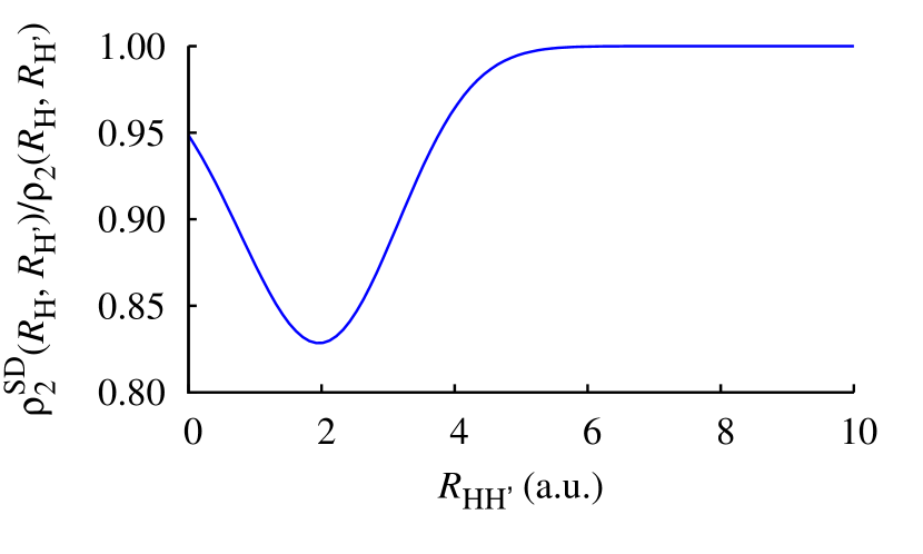
Figure 1: $\rho_{2}^{\text{SD}}(R_{{\text{H}}},R_{{\text{H}}^{\prime}})/\rho_{2}(R_{{\text{H}}},R_{{\text{H}}^{\prime}})$ against the interatomic separation $R_{{\text{H}}{\text{H}}^{\prime}}$ for the minimal basis set calculation of the hydrogen molecule.

Finally, let us mention that the long-range part of $\text{c}_{\textit{II}}$, although very small, it is not exactly zero —as we shall see in the examples covered in the Results section. $\text{c}_{\textit{II}}$ evaluated at $R$, $R$ being the distance between any two atoms in the molecule will decay like $R^{-3}$ when $R\rightarrow\infty$.⁷⁴ This dependency is connected with the well-known $R^{-6}$ decay of the van der Waals (vdW) dispersion energy. Because dispersion interactions are weak, the region in $h_{\text{c}_{\textit{II}}}(s)$ is proportionally small.

3 Computational Details

Full configuration interactions (FCI) calculations have been run with a modified version of Knowles and Handy’s program. ^{87, 88} Dunning’s augmented correlation-consistent double zeta basis set (aug-cc-pVDZ) ^{89, 90} is used unless otherwise specified. We have used the basis sets developed in a previous paper ⁶⁴ for the Be isoelectronic series. The density matrices and the intracule probability distributions have been obtained with the in-house DMN ⁹¹ and RHO2_-OPS ⁹² codes, respectively; the latter uses the algorithm of Cioslowski and Liu. ⁹³

4 Results and discussion

4.1 H₂ in minimal basis

Due to its simplicity, H₂ in a minimal basis (STO-3G)⁹⁴ becomes a perfect model for understanding the partition of the Coulomb hole. Let us consider the equilibrium and a stretched geometry. In both cases, the Coulomb hole is negative at the short range, indicating that HF overestimates the number of electron pairs at short interelectronic distances (see Figure 2). The hole of H₂ at equilibrium becomes positive for values of $s$ larger than the bond length, due to HF’s underestimation of number of electron pairs at these interelectronic distances. The $c_{I}$ part of the hole is positive and rather small, whereas $c_{II}$ accounts for almost the entire shape of the Coulomb hole. The latter indicates that the role of nondynamic correlation is small at equilibrium. At the stretched geometry, the magnitude of the Coulomb hole is considerably larger, and the maximum of the hole coincides with the maximum of the intracule of the pair density. In this case, HF does a worse job describing the distribution of electron pairs, providing significant errors on both the short- and long-range components of the Coulomb hole. As a result of the separability problem, which originates from the impossibility to separate two electrons occupying the same orbital on a restricted single-determinant wavefunction, ² HF underestimates the number of electron pairs formed at large electron-electron separations and overestimates the number of pairs formed at short separations (see Figure 3). Interestingly, the two components of the Coulomb hole provide a clear-cut separation of both phenomena: $c_{I}$ corresponds to the electron pairs missed by HF at long ranges and $c_{II}$ corrects the overestimation of electron pairing at short range. Since the Coulomb hole is the correction to HF’s two-electron distribution, its energetic contribution to the total energy can be regarded as the correction to the HF electron-electron repulsion. In this sense, although $\text{c}_{I}$ contribution is the largest, both hole components contribute to the correlation repulsion energy. The $\text{c}_{I}$ contribution is thus small and comes entirely from the short-range part (which is not apparent in Figure 2, unless we plot $h_{\text{c}_{I}}(s)/s$) because $h_{\text{c}_{I}}(s)/s$ tends to zero for large $s$ as we reach the dissociation limit. Conversely, other properties based on the pair density, such as the covariance of the electron populations of the two H atoms, ⁹⁵ are affected by the value of $\text{c}_{I}$ at all ranges; for these properties, correctly retrieving $h_{\text{c}_{I}}(s)$ at short ranges would not be enough.

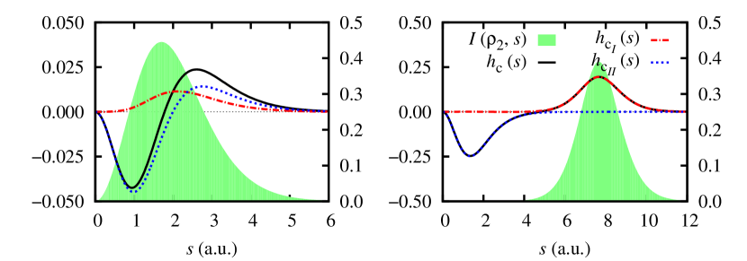
Figure 2: Coulomb hole (black), $h_{\text{c}_{I}}(s)$ (red) and $h_{\text{c}_{II}}(s)$ (blue) correlation components, and the intracule density (green shadowed region, right $y$-axis) of ${}^{1}\Sigma^{+}_{u}$ H₂ calculated with STO-3G basis set at the equilibrium distance (1.39 a.u.) and at 7.56 a.u..

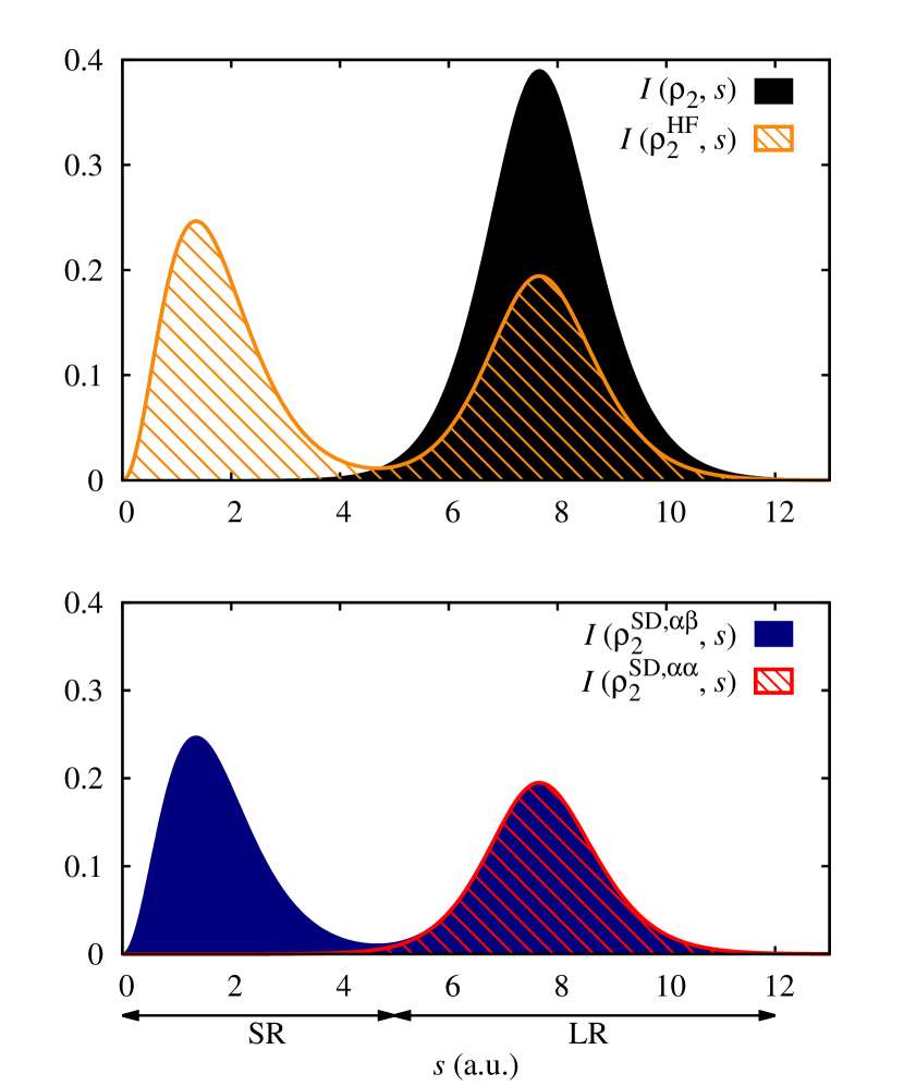
Figure 3: The intracule probability densities of H₂ at $R$ = 7.56 a.u. bond distance calculated with the STO-3G basis set. Top: the exact (filled black) and the Hartree–Fock (dashed orange) intracules. Bottom: the opposite- (filled blue) and same-spin (dashed red) components of the SD pair density approximation intracule. The filling has been included as a visualization aid.

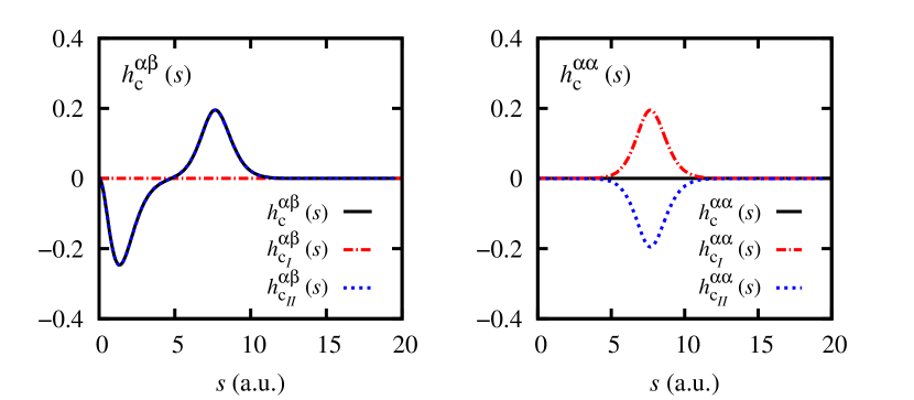
Figure 4: The opposite-spin (left) and same-spin (right) components of the FCI/STO-3G Coulomb hole ($h_{\text{c}}$), $h_{\text{c}_{I}}(s)$ (red) and $h_{\text{c}_{II}}(s)$ (blue) correlation components of H₂ at $R$ = 7.56 a.u..

Let us now dissect the hole and its components into spin contributions for the stretched geometry (see Figure 4). The ground state of H₂ has one electron of each spin; thus, the same-spin contributions of the Coulomb hole are zero, $h_{\text{c}}^{\alpha\alpha}(s)=0$. However, the same-spin contribution of the correlation components of the Coulomb hole, $h^{\alpha\alpha}_{\text{c}_{\textit{I}}}(s)$ and $h^{\alpha\alpha}_{\text{c}_{\textit{II}}}(s)$, is not zero. The latter reveals that the Coulomb hole components do not have any physical meaning; they are simply mathematical objects defined for convenience. Indeed, the so-defined $h_{\text{c}_{I}}(s)$ of H₂ at dissociation arises uniquely from $h^{\alpha\alpha}_{\text{c}_{\textit{I}}}(s)$, which completely reproduces the long-range behavior of the total Coulomb hole. Conversely, $h^{\alpha\beta}_{\text{c}_{\textit{I}}}(s)$ is very small by definition, because neither HF nor SD pair densities explicitly introduce opposite-spin correlation, and the difference between HF and the exact density is expected to be small (in the present case, where we employ a minimal basis set, the density difference is zero in the limit of H₂ dissociation). The long-range opposite-spin correlation is indirectly introduced in the $c_{I}$ component through the addition of the $h^{\alpha\alpha}_{\text{c}_{\textit{I}}}(s)$ contribution. Obviously, for systems of only one alpha electron, $h^{\alpha\alpha}_{\text{c}_{\textit{I}}}(s)=-h^{\alpha\alpha}_{\text{c}_{\textit{II}}}(s)$ and, therefore, $h^{\alpha\alpha}_{\text{c}_{\textit{II}}}(s)$ is compensating for the long-range contribution of $h^{\alpha\beta}_{\text{c}_{\textit{II}}}(s)$, making $h_{\text{c}_{\textit{II}}}(s)$ short-ranged. In other words, $h_{c_{I}}(s)$ captures the long-range component of the Coulomb hole through the intracule of $\rho_{2}^{\text{SD},\alpha\alpha}(\boldsymbol{1},\boldsymbol{2})$. In particular, the latter contributes a quadratic term on $r_{12}$ at short ranges, and its long-range contribution is dominated by the $\rho^{\alpha}(\boldsymbol{1})\rho^{\alpha}(\boldsymbol{2})$ term in $\rho_{2}^{\text{SD},\alpha\alpha}(\boldsymbol{1},\boldsymbol{2})$. Hence, as a first approximation to the long-range part of $\Delta\rho_{2}^{c_{I}}(\boldsymbol{1},\boldsymbol{2})$ one could take $\rho^{\alpha}(\boldsymbol{1})\rho^{\alpha}(\boldsymbol{2})+\rho^{\beta}(\boldsymbol{1})\rho^{\beta}(\boldsymbol{2})$, which captures the long-range asymptotics of the Coulomb hole.

4.2 H₂ triplet: dispersion interactions

The triplet state of H₂ (${}^{3}\Sigma_{u}^{+}$) is composed solely of two electrons with the same spin and constitutes probably the simplest model to study dispersion interactions. ⁹⁶ In contrast to the ground state singlet (${}^{1}\Sigma_{u}^{+}$), the triplet state ${}^{3}\Sigma_{u}^{+}$ (with spin projection either $M_{s}=1$ or $M_{s}=-1$) is qualitatively well described by the HF configuration at any interatomic distance and bears the correct dissociation. ⁹⁷ Indeed, compared to the singlet, the Coulomb hole is very small (see the left $y$-axis in Figure 5). This case does not present electron entanglement, therefore, nondynamic correlation does not arise when the two fragments are separated.

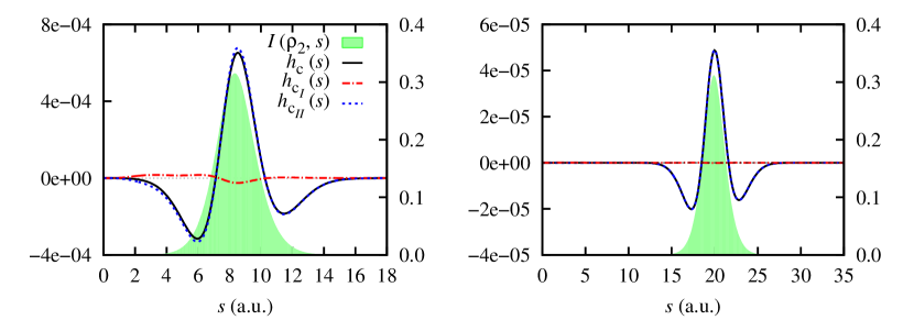
Figure 5: Coulomb hole (black), $h_{\text{c}_{I}}(s)$ (red) and $h_{\text{c}_{II}}(s)$ (blue) correlation components, and the intracule density (green shadowed region, right $y$-axis) of the ${}^{3}\Sigma_{u}^{+}$ state of H₂ molecule at 8.18 (left) and at 19.84 a.u. (right).

Long-range dispersion interactions are considered because we have employed a basis set including $p$ orbitals. ⁹⁸ The only peak in the Coulomb hole corresponds to dispersion interactions and, thus, it is captured by $h_{\text{c}_{\textit{II}}}(s)$.⁷⁴ $h_{\text{c}_{\textit{II}}}(s)$ peaks around the interatomic separation, $R_{\text{HH}^{\prime}}$, indicating that HF underestimates the number of electron pairs at $R_{\text{HH}^{\prime}}$, which are placed at shorter and longer distances. On the other hand, there is almost no $h_{\text{c}_{\textit{I}}}(s)$ contribution at equilibrium, and it is zero at the stretched geometry. The latter is due to $\rho_{2}^{\text{SD}}(\boldsymbol{1},\boldsymbol{2})$ being very close to $\rho_{2}^{\text{HF}}(\boldsymbol{1},\boldsymbol{2})$, which results from the small changes induced by electron correlation into the density or the first-order density. As we have recently proved, ^{74, 22} dispersion interactions are characterized by a universal feature: $h_{\text{c}_{\textit{II}}}(R_{\text{HH}^{\prime}})$ decays as $R_{\text{HH}^{\prime}}^{-3}$ for large $R_{\text{HH}^{\prime}}$.

4.3 He-Ne atomic series

Since correlation increases with the number of electrons, the Coulomb hole is expected to increase with the atomic number, $Z$. The magnitude of the hole increases and shrinks with $Z$, whereas $\langle s\rangle$ decreases due to a larger attractive potential. However, the latter increase is not monotonic (see the plot for $h_{\text{c}}(s)$ in Figure S4). The splitting of the hole into the two correlation components reveals that $h_{\text{c}_{II}}(s)$ presents a systematic growth with $Z$ (see the magnitude increase in the top plot of Figure 6). Conversely, $h_{\text{c}_{I}}(s)$ reveals characteristic shapes according to the nature of each atom, in agreement with the expected nondynamic correlation behavior in these systems (bottom plot in Figure 6).

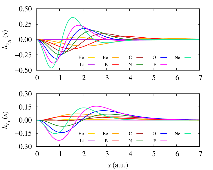
Figure 6: $h_{\text{c}_{II}}$ (top) and $h_{\text{c}_{I}}$ (bot) correlation components of the Coulomb hole of the He-Ne atomic series in their lowest-lying multiplicities.

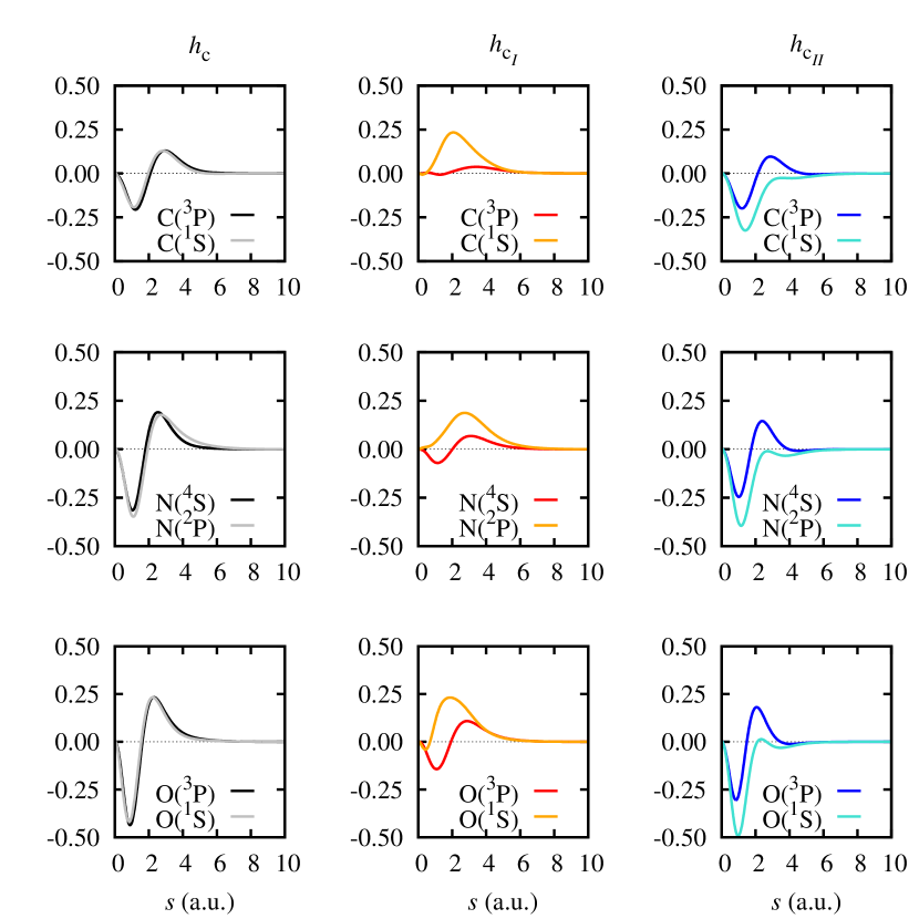
Figure 7: $h_{\text{c}}(s)$, $h_{\text{c}_{I}}(s)$, and $h_{\text{c}_{II}}(s)$ of carbon, nitrogen, and oxygen in their ground state (black, red and blue, respectively) and minimum multiplicity state (gray, orange and turquoise).

We have studied different multiplicities for carbon, nitrogen, and oxygen: their lowest-lying states (highest-spin multiplicity) and the states with the lowest multiplicity. Their holes are compiled in Figure 7. The most outstanding feature is that the Coulomb hole of all the atoms looks practically identical regardless of the multiplicity (see the first column of Figure 8) and, therefore, one expects a similar correlation contribution to the electron-electron repulsion. The nature of electron correlation is different for the various state multiplicities; therefore, we can conclude that a mere analysis of the shape of the Coulomb hole does not provide insight into the electron correlation of these systems. Conversely, the Coulomb hole components display different shapes according to the spin state.

More precisely, each state presents a characteristic profile, independently of the atom considered. In the ground states (highest-spin multiplicities), both $\text{c}_{\textit{I}}$ and $\text{c}_{\textit{II}}$ components present the conventional hole shape, being negative at short interelectronic distances and positive at large ones. $h_{{c}_{\textit{II}}}(s)$ is, in general, larger than $h_{\text{c}_{I}}(s)$ and both increase systematically with the number of electrons (see Figure 7) —in line with the fact that the HF description loses accuracy from C to O. Conversely, the atoms in their lowest spin multiplicity present mostly positive ${h_{\text{c}_{I}}}(s)$ and short-ranged negative $h_{\text{c}_{\textit{II}}}(s)$.

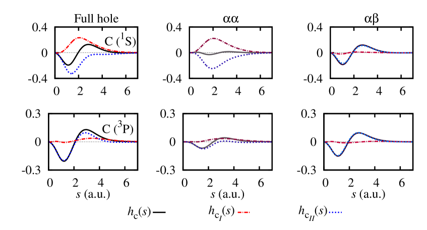
Figure 8: The Coulomb hole, $h_{\text{c}}(s)$, and its correlation components, $h_{\text{c}_{I}}(s)$ and $h_{\text{c}_{II}}(s)$, (left column), the $\alpha\alpha$ (middle column) and $\alpha\beta$ contributions to the Coulomb hole (right column) for singlet state carbon (top row) and the triplet, ground state (bottom row).

The reason behind these characteristic profiles is explored through the spin decomposition of the holes. We have used the carbon atom to illustrate it. As we can see in Figure 8, the spin components of the Coulomb hole present similar profiles in singlet carbon (C(¹S)) and singlet H₂ (compare to Figure 4). The shape of the Coulomb hole is mainly given by the opposite-spin $h_{\text{c}_{II}}(s)$ component, and the same-spin components are more important in the description of the singlet than in the triplet. The latter feature can be explained from the nature of $\rho_{2}^{\alpha\alpha,\text{SD}}(\boldsymbol{1},\boldsymbol{2})$, which contributes to $h^{\alpha\alpha}_{\text{c}_{I}}(s)$. Since $h^{\alpha\alpha}_{\text{c}_{I}}(s)$ is greater than zero, its magnitude can be related to the inability of $\rho_{2}^{\alpha\alpha,\text{SD}}(\boldsymbol{1},\boldsymbol{2})$ to reproduce the number of electron pairs of the same spin upon integration over $\boldsymbol{1}$ and $\boldsymbol{2}$. The more considerable the electron correlation effects on the first-order density, the larger the deviation from the number of electron pairs of the same spin.⁹⁹ Therefore, singlet carbon, which is much more affected by nondynamic correlation, presents larger values of $h^{\alpha\alpha}_{\text{c}_{I}}(s)$ and, since the total Coulomb hole is mainly given by the opposite-spin component, $h^{\alpha\alpha}_{\text{c}_{II}}(s)$ will be large and (partially) compensate for $h^{\alpha\alpha}_{\text{c}_{I}}(s)$ (see Figure 8). Table 1 shows that the trace deviation of the like-spin SD pair density is larger in the singlet than in the triplet.

	Ne	C(3P)	C(1S)
Tr$\left[\rho_{2}^{\alpha\alpha}\left(\boldsymbol{1},\boldsymbol{2}\right)\right]$	20.00	7.00	6.00
Tr$\left[\rho_{2}^{\alpha\alpha,\text{SD}}\left(\boldsymbol{1},\boldsymbol{2}\right)\right]$	20.06	7.11	6.59

Table 1: Same-spin pair-density traces for Ne, the singlet and triplet states of carbon atom. Tr$\left[\rho_{2}^{\alpha\alpha}\left(\boldsymbol{1},\boldsymbol{2}\right)\right]=N^{\alpha}\left(N^{\alpha}-1\right)$.

4.4 The Be₂ Coulomb hole

The description of both Be atom and its dimer is very sensitive to the level of theory and the quality of the basis set employed¹⁰⁰ (see also Supporting Information, where we follow a previous strategy ^{88, 101, 64} to analyze the effect of the basis set). Due to the well-known near-degeneracy of $2s$ and $2p$ orbitals in Be, the binding of both fragments and, in general, the potential energy curve (PEC) of Be₂ has been the subject of study of both experimentalists and computational chemists alike. One of the most intriguing features of the PEC of Be₂ is a change of slope that generates two potential minima, one corresponding to the equilibrium geometry at $4.72$ a.u., and the second one at twice the equilibrium distance. Because of this double well, a single-reference method with a basis set that includes neither $d$ nor $f$ functions usually gives the second geometry as the equilibrium one, or even a repulsive, non-binding curve. ^{102, 103, 104} In our study, we have run a frozen-core full configuration interaction (FCI) calculation with the aug-cc-pVTZ basis set to study the Coulomb hole. It has been shown elsewhere ¹⁰³ that the core electrons do not play an important role in the electronic description of Be₂ because the triple and quadruple excitations of the valence electrons are the ones responsible for most electron correlation.

Figure 9 contains the Coulomb holes of two geometries of Be₂. Two interesting features of $h_{\text{c}}(s)$ are the presence of a small bump around the hole evaluated at the interatomic distance, $h_{\text{c}}(s=R)$, and a shoulder at the small $s$ region for both geometries. The latter is connected with the lack of correlation of the core electrons (see the magnification in Figure S2 and Ref. 64 for a discussion on the effect of core electrons in the Coulomb hole). For both geometries, $h_{\text{c}_{I}}(s)$ takes large numbers due to the nondynamic correlation arising from the near-degeneracy of the $2s$ and $2p$ orbitals of the beryllium atom; this multireference character is preserved in the dimer. It has actually been reported that the valence molecular orbitals $3\sigma_{g}$ and $3\sigma_{u}$, which arise from linear combinations of $2s$ and $2p$, show relatively large orbital occupation numbers and, hence, should be considered in the calculation.^{103, 104} Indeed, the FCI occupation number of both $3\sigma_{g}$ and $3\sigma_{u}$ is 0.0589 at $R=$ 24.57 a.u.. Conversely, since the $2\sigma$ orbitals are occupied in the HF description, it cannot provide an accurate 1-RDM at this stretched geometry and, therefore, $\Delta\rho_{2}^{\text{c}_{I}}(\boldsymbol{1},\boldsymbol{2})$ is large. Certainly, the wrong dissociation provided by HF and the strong multireference character of the dissociated Be fragments make the HF 1-RDM a very poor reference. The long-range part of the Coulomb hole of stretched Be₂ presents a maximum that belongs to $h_{\text{c}_{\textit{I}}}(s)$, caused by the presence of the valence electrons localized near the respective nuclei. The long-range part of $h_{\text{c}_{\textit{II}}}\left(s\right)$ in stretched Be₂ presents a minuscule yet positive area due to dispersion interactions.

The most remarkable feature of the Coulomb hole splitting of this molecule is the dominance of both types of correlation at short range. In most of the cases studied thus far, the short-range part of the Coulomb hole has always been dominated by $h_{\text{c}_{\textit{II}}}(s)$, which defined the shape of the short-range part of the total hole $h_{\text{c}}(s)$. At the equilibrium and stretched geometries, the short-range part of the total hole of Be₂ is molded by both correlation contributions.

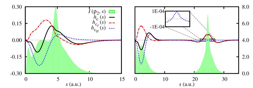
Figure 9: Coulomb hole (black), $h_{\text{c}_{I}}(s)$ (red) and $h_{\text{c}_{II}}(s)$ (blue) correlation components, and the intracule density (green shadowed region, right $y$-axis) of the Be₂ molecule at 4.72 a.u. (left) and 24.57 a.u. (right) bond lenghts.

4.5 Types A and B of nondynamic correlation: Be(Z) and H₂

Hollett and Gill recognized two types of nondynamic correlation that are classified according to the ability of the unrestricted Hartree–Fock (UHF) method to capture them. ¹¹ The first type, type A, arises from absolute near degeneracies, for example, those that occur when a homolytic dissociation takes place. As the interatomic separation distance $R$ increases, the energy gap ($\epsilon_{gap}$) between the highest occupied and lowest unoccupied molecular orbitals (HOMO and LUMO, respectively) becomes smaller until it vanishes and these orbitals become degenerate. Certainly, RHF cannot describe the localization of the electrons at each nucleus, whereas the unrestricted formalism succeeds in doing so by getting rid of the ionic description. The second type, named type B, arises in the presence of relative near-degeneracies. The HOMO-LUMO gap widens in the Be isoelectronic series as the effective charge $Z$ increases. However, the difference between gap increments, $\Delta\epsilon_{gap}$, remains constant. UHF cannot portray the nondynamic correlation in this scenario, and multireference methods are required for an accurate description. Identifying correlation types A and B is a challenging test for correlation indicators.²⁰ The present section studies whether correlation types A and B can be detected by $h_{\text{c}_{\textit{I}}}(s)$. Namely, we analyze a typical case of type B correlation, the isoelectronic series of Be, Be($Z$) with $Z$ = 3–8, and the dissociated and equilibrium geometries of H₂ as an example of type A correlation.

Many studies on the consistency and convergence of basis sets using the Be atom exist in the literature, reflecting the difficulty to correctly reproduce the short-range interactions in this system. ^{105, 102} We have optimized an even-tempered basis set of 10 s, p, and d functions to perform the calculations of Be($Z$). Information about the optimization is provided in the Supporting Information.

It has been demonstrated elsewhere that the correlation energy in Be grows linearly with $Z$ due to the $2s-2p$ near-degeneracy.¹⁰⁶ Consequently, the energy difference between UHF and RHF, $\Delta E$, is expected to increase with $Z$. Instead, Hollet and Gill demonstrated the contrary in their work: the molecules present a triplet instability and UHF can describe nondynamic correlation from $Z$ = 3.0 to $Z$ = 4.25, yielding lower total energies with respect to RHF. Conversely, the fraction of energy recovered by UHF decreases as $Z$ increases, and the UHF description in $5\leq Z\leq 8$ is equivalent to the RHF one (see Table 2). The HOMO-LUMO gap widens with the effective charge $Z$, but the difference between gaps, $\Delta\epsilon_{\text{gap}}$, remains constant, indicating a linear gap growth.

$Z$	$E_{\text{RHF}}$	$E_{\text{UHF}}$	$\Delta E$	$\langle S^{2}\rangle_{\text{UHF}}$	$\epsilon_{\text{HOMO}}$	$\epsilon_{\text{LUMO}}$	$\epsilon_{\text{gap}}$	$\Delta\epsilon_{\text{gap}}$
3	-7.38012	-7.39086	-0.01074	0.7132	0.04521	0.02639	0.21864	0.15874
4	-14.57022	-14.57059	-0.00036	0.1378	-0.31300	0.06438	0.37738	0.22385
5	-24.23339	-24.23339	0.00000	0.0000	-0.87412	-0.27289	0.60123	0.22636
6	-36.39601	-36.39601	0.00000	0.0000	-1.69410	-0.86651	0.82759	0.22368
7	-57.07217	-57.07217	0.00000	0.0000	-2.76685	-1.71558	1.05127	0.21915
8	-68.22939	-68.22939	0.00000	0.0000	-4.08835	-2.81793	1.27042	-

Table 2: The Restricted Hartree–Fock energy, Unrestricted Hartree–Fock energy, their energy difference, the spin contamination from the UHF calculation, the HOMO and LUMO energies and their difference, and the difference between energy gaps for Be-like ions with $3\leq Z\leq 8$.

Figure 10 contains the $h_{\text{c}_{I}}(s)$ contribution for Be-like ions with $3\leq Z\leq 6$. The numbers displayed in Table 2 and Ref. 11 show that a broken symmetry solution does not exist for $Z$ = 5 and 6 and, hence, the UHF and RHF holes are indistinguishable. The UHF and RHF holes for the Be atom are quite similar, whereas for $Z$ = 3 both descriptions are no longer equivalent.

Figure S3 of the Supporting Information provides the Coulomb hole decomposition of a UHF calculation of the H₂ with a minimal basis set. The latter is barely indistinguishable from the FCI counterpart (Figure 2), indicating that $h_{\text{c}_{I}}(s)$ also accounts for type A correlation. In fact, we can easily prove analytically that the FCI and UHF pair density and the 1-RDM are identical in a minimal basis set. From the examples in this section, we conclude that $h_{\text{c}_{I}}(s)$ can describe nondynamic correlation, regardless of its type.

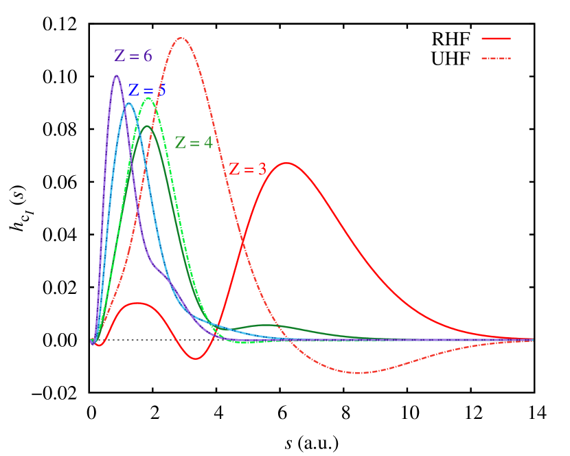
Figure 10: $h_{\text{c}_{I}}(s)$ component of the Coulomb hole of Be-like atoms, Be($Z$), with $Z$ = 3, 4, 5 and 6. Solid (dashed) lines depict the holes described using as reference the restricted (unrestricted) formalism of Hartree–Fock, that is, $h_{\text{c}_{I}}(s)=I\left(\rho_{2}^{\text{SD}},s\right)-I\left(\rho_{2}^{\text{RHF}},s\right)$ for solid lines, and $h_{\text{c}_{I}}(s)=I\left(\rho_{2}^{\text{SD}},s\right)-I\left(\rho_{2}^{\text{UHF}},s\right)$ for dashed lines.

4.6 C_3v-H₄

We consider the three lowest-lying states of the C_3v PEC of H₄ constructed by displacing one H (hereafter, the axial H or H${}_{\text{ax}}$) in the direction perpendicular to the equatorial plane where the rest of H atoms are located (see Figure 11). ^{107, 108, 109, 110, 111, 112, 113} The distance between the equatorial hydrogens ($R_{\text{H}_{{\Delta}}}$) is kept fixed at 1.77 a.u.. ¹¹¹

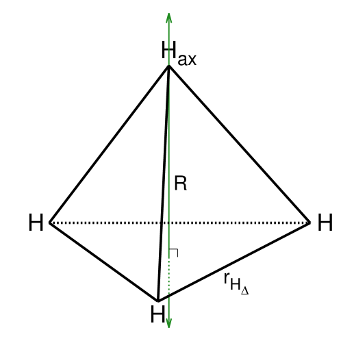
Figure 11: Graphical representation of H₄ at the C_3v symmetry point group, where the position of the axial hydrogen (H${}_{\text{ax}}$) through the axial axis $R$ (marked as green) represents the PEC analyzed. We keep r${}_{H_{\Delta}}$ fixed at 1.77 a.u.. $R$ = 0 when H${}_{\text{ax}}$ is at the equatorial plane.

The FCI PEC presents an intersystem crossing around $R$ = 4.50 a.u. from S₀ to state S₁ (see Figure 12). At the S₀ state, the system is described as two interacting H₂ molecules. The increase of $R$ causes one of these molecules to dissociate, leaving H${}_{3}^{+}$ in the equatorial plane and an H^-, the dissociated hydride (H${}_{\text{ax}}$). The HF description of $S_{0}$ at the ground state is dominant in the CI vector, and the largest occupation numbers of the natural orbitals are 1.957 and 1.936. Conversely, at $R$ = 28.35 a.u. (S₁), the CI vector comprises at least four highly contributing configurations, and the natural occupations are 1.954, 1.000, 0.992, and 1.000, the latter corresponding to H${}_{\text{ax}}$.

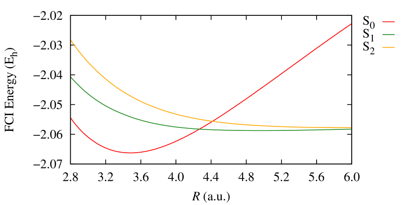
Figure 12: C_3v PECs of H₄, where the coordinate axis represents the separation of the axial hydrogen H${}_{\text{ax}}$ from the plane. A crossing from S₀ to S₁ takes place at 4.27 a.u.

The magnitudes of the Coulomb holes at the equilibrium and dissociated geometries reflect the changes in the CI vector, where the S₁ state is more correlated than S₀. The correlation contributions depicted in Figure 13 show that $h_{\text{c}_{\textit{II}}}(s)$ is prevalent at the equilibrium geometry and defines the shape of the Coulomb hole. At the stretched geometry, however, the short-range part of the Coulomb hole is dominated by $h_{\text{c}_{\textit{I}}}(s)$, mainly caused by the multireference description of the S₁ state that results from the spin frustration of the three hydrogens that remain on the same plane. $h_{\text{c}_{\textit{II}}}(s)$ retains a simple shape and presents a long-range peak caused by the dispersion interaction between H${}_{\text{ax}}$ and the rest of the hydrogens in the plane. $h_{\text{c}_{\textit{I}}}(s)$ at the stretched geometry presents two features we have not seen thus far in this component of the Coulomb hole: it has a substantial value at short ranges and shows important negative values at long ranges. These unique features of $h_{\text{c}_{\textit{I}}}(s)$ put forward the very deficient description of HF, which does not dissociate into fragments with an integer number of electrons. If HF dissociated into the correct number of electrons for each fragment, the shape of $h_{\text{c}_{\textit{I}}}(s)$ would not show these features (compare to the Coulomb hole in Figure S6, which uses UHF as a reference). The positive short-range part of $h_{\text{c}_{\textit{I}}}(s)$ reflects the excess of electrons that HF locates in the H₃ plane. HF also locates less than one electron in H${}_{\text{ax}}$, resulting in the negative long-range part of $h_{\text{c}_{\textit{I}}}(s)$.

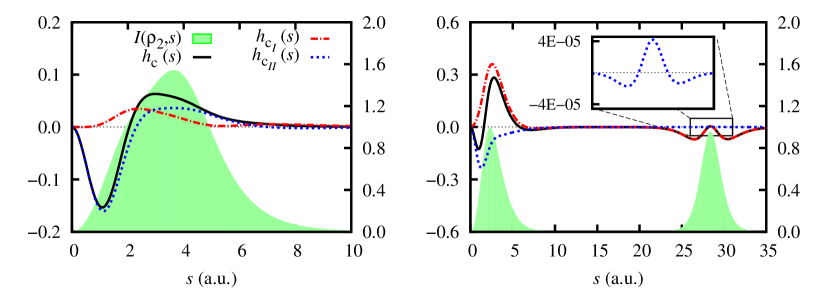
Figure 13: Coulomb hole (black), $h_{\text{c}_{I}}(s)$ (red) and $h_{\text{c}_{II}}(s)$ (blue) correlation components, and the intracule density (green shadowed region, right $y$-axis) of H₄ molecule at the C_3v symmetry point group with fixed r${}_{\text{H}_{\Delta}}$. H${}_{\text{ax}}$ is placed at (left) $R$ = 3.50 a.u. (right) and $R$ = 28.35 a.u. from the equatorial plane (see Figure 11 for details).

4.7 LiH and the harpoon mechanism

LiH has an ionic ground state and its lowest-lying excited state is covalent. ¹¹⁴ Thus, in the adiabatic representation, the ground state of LiH presents an ionic bonding at equilibrium, with Li⁺ and H^-, whereas the character of the state changes from ionic to covalent as the molecule dissociates (see Figure 14). The mechanism depicting the electron transition from hydrogen to lithium is known as the harpoon mechanism,¹¹⁵ and it is caused by the small ionization potential of lithium and the large electron affinity of hydrogen. The potential energy curve presents an avoided crossing where the transition from the covalent state to the ionic description occurs ($R_{Li-H}=6.8$). ¹¹⁴

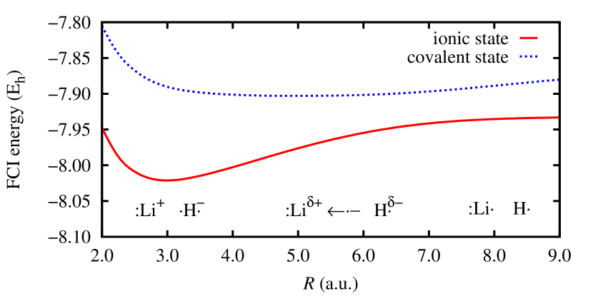
Figure 14: PECs of the lowest-lying diabatic states in LiH. An avoided crossing takes places around 6.8 a.u. Below, the harpoon mechanism is depicted.

Two different profiles, which resemble the C_3v-H₄ profiles depicted in Figure 13, are obtained at different distances (see Figure 15). Although HF correctly describes the ionic equilibrium geometry, the covalent character of the state at large interatomic distances is not well represented. Therefore, the Coulomb hole at equilibrium does not differ qualitatively from the hole of other molecules, such as H₂. On the other hand, $h_{\text{c}_{\textit{I}}}(s)$ is predominant along the interelectronic distance coordinate for the stretched geometry. $h_{\text{c}_{\textit{II}}}(s)$ displays moderate values at short range and is inappreciable at long range for the stretched LiH. As we can see in the inset plot, $h_{\text{c}_{\textit{II}}}(s)$ is characterized by a maximum, which features the universal signature of dispersion. HF also dissociates LiH into fragments with a non-integer number of electrons; therefore, the resemblance between this hole and the one of H₄. In fact, at the stretched geometry, the difference between the exact intracular and the UHF one is negligible (see Figure S5), indicating that all the features of the Coulomb hole in Figure 15 are entirely due to the wrong dissociation of HF. ^{74, 22}

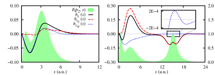
Figure 15: Coulomb hole (black), $h_{\text{c}_{I}}(s)$ (red) and $h_{\text{c}_{II}}(s)$ (blue) correlation components, and the intracule density (green shadowed region, right $y$-axis) of LiH at the equilibrium geometry (3.02 a.u.), and at 15.12 a.u..

5 Conclusions

We have studied a correlation decomposition scheme that provides a natural separation of the pair density. The Coulomb hole’s range separation into two components, $h_{\text{c}_{I}}(s)$ and $h_{\text{c}_{II}}(s)$, arises after integrating the extracule coordinate. The c${}_{\textit{I}}$ component describes nondynamic long-range correlation interactions, whereas the c${}_{\textit{II}}$ component features dynamic and nondynamic short-range interactions. These components are exhaustively analyzed throughout various examples that put forward the most relevant features of this approach.

First of all, through the asymptotic properties of the hole parts, we explain how the component based only on the first-order reduced density matrix (c${}_{\textit{I}}$) can retrieve the long-range part of electron correlation. Second, we perform an exhaustive analysis of the hydrogen molecule in a minimal basis set, dissecting the hole contributions into spin components. Third, we analyze the simplest molecule presenting a dispersion interaction, triplet H₂, and how $h_{\text{c}_{II}}(s)$ helps identify it. This dispersion signature is also present in all the other molecules studied in this work, highlighting its universal character. We also analyze the Coulomb holes of several atoms in different spin states, finding that the hole components distinguish correlation regimes that are not apparent from the entire hole. Indeed, atoms with different spin states present the same Coulomb hole profile but its c${}_{\textit{I}}$ component gives away the true multireference character of the singlet state of carbon and nitrogen atoms.

Finally, we analyze the two types of nondynamic correlation, types A and B,¹¹ and show that c${}_{\textit{I}}$ can capture them. Profiles of $h_{\text{c}_{\textit{I}}}(s)$ calculated with an unrestricted reference differ from profiles calculated with a restricted wavefunction when type B nondynamic correlation is present. The more important the type B correlation, the more significant the difference between both holes. Interestingly, the correlation indicators based on natural orbitals that were also developed from this partition²⁰ could not make such a distinction.

The results of this work hold the promise to aid in developing new electronic structure methods that efficiently capture electron correlation. In particular, the models of the $c_{II}$ component can be combined with other results available in the literature^{73, 58, 57} to develop new approximations in the reduced density matrix functional theory,^{54, 55} although the present work is not limited to this theory.

Conflicts of interest

There are no conflicts to declare.

References

- Löwdin 1955 P.-O. Löwdin, Phys. Rev., 1955, 97, 1474–1489.
- Szabo and Ostlund 2012 A. Szabo and N. S. Ostlund, Modern Quantum Chemistry: Introduction to Advances Electronic Structure Theory, Courier Corporation, New York, 2012.
- Wilson 2007 S. Wilson, Electron correlation in molecules, Dover, New York, 2007.
- Hättig et al. 2012 C. Hättig, W. Klopper, A. Köhn and D. P. Tew, Chem. Rev., 2012, 112, 4–74.
- Tew et al. 2007 D. P. Tew, W. Klopper and T. Helgaker, J. Comput. Chem., 2007, 28, 1307–1320.
- Cremer 2001 D. Cremer, Mol. Phys., 2001, 99, 1899–1940.
- Ziesche 2000 P. Ziesche, J. Mol. Struct. (Theochem), 2000, 527, 35–50.
- Raeber and Mazziotti 2015 A. Raeber and D. A. Mazziotti, Phys. Rev. A, 2015, 92, 052502.
- Benavides-Riveros et al. 2017 C. L. Benavides-Riveros, N. N. Lathiotakis, C. Schilling and M. A. Marques, Phys. Rev. A, 2017, 95, 032507.
- Gottlieb and Mauser 2005 A. D. Gottlieb and N. J. Mauser, Phys. Rev. Lett., 2005, 95, 123003.
- Hollett and Gill 2011 J. W. Hollett and P. M. Gill, J. Chem. Phys., 2011, 134, 114111.
- Fogueri et al. 2013 U. R. Fogueri, S. Kozuch, A. Karton and J. M. L. Martin, Theor. Chem. Acc., 2013, 132, 1–9.
- Proynov et al. 2013 E. Proynov, F. Liu and J. Kong, Phys. Rev. A, 2013, 88, 032510.
- Cioslowski 1991 J. Cioslowski, Phys. Rev. A, 1991, 43, 1223–1228.
- Valderrama et al. 1997 E. Valderrama, E. V. Ludeña and J. Hinze, J. Chem. Phys., 1997, 106, 9227–9235.
- Valderrama et al. 1999 E. Valderrama, E. V. Ludeña and J. Hinze, J. Chem. Phys., 1999, 110, 2343–2353.
- Mok et al. 1996 D. K. W. Mok, R. Neumann and N. C. Handy, J. Phys. Chem., 1996, 100, 6225–6230.
- Benavides-Riveros et al. 2017 C. L. Benavides-Riveros, N. N. Lathiotakis and M. A. Marques, Phys. Chem. Chem. Phys., 2017, 19, 12655–12664.
- Vuckovic et al. 2017 S. Vuckovic, T. J. P. Irons, L. O. Wagner, A. M. Teale and P. Gori-Giorgi, Phys. Chem. Chem. Phys., 2017, 19, 6169–6183.
- Ramos-Cordoba et al. 2016 E. Ramos-Cordoba, P. Salvador and E. Matito, Phys. Chem. Chem. Phys., 2016, 18, 24015–24023.
- Ramos-Cordoba and Matito 2017 E. Ramos-Cordoba and E. Matito, J. Chem. Theory Comput., 2017, 13, 2705–2711.
- Via-Nadal et al. 2019 M. Via-Nadal, M. Rodríguez Mayorga, E. Ramos-Cordoba and E. Matito, J. Phys. Chem. Lett., 2019, 10, 4032–4037.
- Bartlett and Musiał 2007 R. J. Bartlett and M. Musiał, Rev. Mod. Phys., 2007, 79, 291.
- Sinanoğlu 1964 O. Sinanoğlu, Adv. Chem. Phys., 1964, 6, 315–412.
- Stone 2013 A. J. Stone, The theory of intermolecular forces, Oxford University Press, 2nd edn., 2013.
- Shavitt 1977 I. Shavitt, in Methods of electronic structure theory, Springer, 1977, pp. 189–275.
- Čížek 1966 J. Čížek, J. Phys. Chem., 1966, 45, 4256–4266.
- Møller and Plesset 1934 C. Møller and M. S. Plesset, Phys. Rev., 1934, 46, 618.
- Kohn and Sham 1965 W. Kohn and L. J. Sham, Phys. Rev., 1965, 140, A1133–A1138.
- Helgaker et al. 2000 T. Helgaker, P. Jørgensen and J. Olsen, Molecular Electronic-Structure Theory, John Wiley & Sons, Ltd, Chichester, 2000.
- Roos 1987 B. O. Roos, Adv. Chem. Phys., 1987, 69, 399–445.
- White and Huse 1993 S. R. White and D. A. Huse, Phys. Rev. B, 1993, 48, 3844.
- Frenkel 1934 J. Frenkel, Wave Mechanics, Volume 2: Advanced General Theory, The Clarendon Press, Oxford, 1934, pp. 460–462.
- Roos and Siegbahn 1977 B. O. Roos and P. Siegbahn, Methods of electronic structure theory, Plenum Press, New York, 1977.
- Andersson et al. 1990 K. Andersson, P.-Å. Malmqvist, B. O. Roos, A. J. Sadlej and K. Wolinski, J. Phys. Chem., 1990, 94, 5483–5488.
- Andersson et al. 1992 K. Andersson, P.-Å. Malmqvist and B. O. Roos, J. Chem. Phys., 1992, 96, 1218–1226.
- Buenker and Peyerimhoff 1974 R. J. Buenker and S. D. Peyerimhoff, Theor. Chim. Acta (Berlin), 1974, 35, 33–58.
- Werner and Knowles 1988 H.-J. Werner and P. J. Knowles, J. Chem. Phys., 1988, 89, 5803–5814.
- Pastorczak et al. 2019 E. Pastorczak, M. Hapka, L. Veis and K. Pernal, J. Phys. Chem. Lett., 2019, 10, 4668–4674.
- Hollett and Loos 2020 J. W. Hollett and P.-F. Loos, J. Chem. Phys., 2020, 152, 014101.
- Piris 2021 M. Piris, Phys. Rev. Lett., 2021, 127, 233001.
- Savin 1996 A. Savin, in Recent Developments of Modern Density Functional Theory, ed. J. M. Seminario, Elsevier: Amsterdam, 1996, p. 327.
- Savin 1988 A. Savin, Int. J. Quantum Chem., 1988, 34, 59–69.
- Fromager et al. 2007 E. Fromager, J. Toulouse and H. J. A. Jensen, J. Chem. Phys., 2007, 126, 074111.
- Toulouse et al. 2009 J. Toulouse, I. C. Gerber, G. Jansen, A. Savin and J. G. Angyán, Phys. Rev. Lett., 2009, 102, 096404.
- Toulouse et al. 2004 J. Toulouse, F. Colonna and A. Savin, Phys. Rev. A, 2004, 70, 062505.
- Iikura et al. 2001 H. Iikura, T. Tsuneda, T. Yanai and K. Hirao, J. Chem. Phys., 2001, 115, 3540–3544.
- Baer et al. 2010 R. Baer, E. Livshits and U. Salzner, Ann. Rev. Phys. Chem., 2010, 61, 85–109.
- Garrett et al. 2014 K. Garrett, X. Sosa Vazquez, S. B. Egri, J. Wilmer, L. E. Johnson, B. H. Robinson and C. M. Isborn, J. Chem. Theory Comput., 2014, 10, 3821–3831.
- Bao et al. 2017 J. J. Bao, L. Gagliardi and D. G. Truhlar, Phys. Chem. Chem. Phys., 2017, 19, 30089–30096.
- Gagliardi et al. 2017 L. Gagliardi, D. G. Truhlar, G. Li Manni, R. K. Carlson, C. E. Hoyer and J. L. Bao, Acc. Chem. Res., 2017, 50, 66–73.
- Li Manni et al. 2014 G. Li Manni, R. K. Carlson, S. Luo, D. Ma, J. Olsen, D. G. Truhlar and L. Gagliardi, J. Chem. Theory Comput., 2014, 10, 3669–3680.
- Coleman 1967 A. J. Coleman, Int. J. Quantum Chem., 1967, 1, 457–464.
- Piris and Ugalde 2014 M. Piris and J. M. Ugalde, Int. J. Quantum Chem., 2014, 114, 1169–1175.
- Pernal and Giesbertz 2015 K. Pernal and K. J. H. Giesbertz, Top. Curr. Chem., 2015, 368, 125–183.
- Ramos-Cordoba et al. 2015 E. Ramos-Cordoba, X. Lopez, M. Piris and E. Matito, J. Chem. Phys., 2015, 143, 164112.
- Ramos-Cordoba et al. 2014 E. Ramos-Cordoba, P. Salvador, M. Piris and E. Matito, J. Chem. Phys., 2014, 141, 234101.
- Cioslowski et al. 2015 J. Cioslowski, M. Piris and E. Matito, J. Chem. Phys., 2015, 143, 214101.
- McWeeny 1989 R. McWeeny, Methods of Molecular Quantum Mechanics, Academic Press, London, 2nd edn., 1989.
- Rodríguez-Mayorga et al. 2018 M. Rodríguez-Mayorga, M. Via-Nadal, M. Solà, J. M. Ugalde, X. Lopez and E. Matito, J. Phys. Chem. A, 2018, 122, 1916–1923.
- Sarasola et al. 1990 C. Sarasola, J. M. Ugalde and R. J. Boyd, J. Phys. B: At. Mol. Opt. Phys., 1990, 23, 1095.
- Sarasola et al. 1992 C. Sarasola, L. Dominguez, M. Aguado and J. Ugalde, J. Chem. Phys., 1992, 96, 6778–6783.
- Mercero et al. 2016 J. M. Mercero, M. Rodríguez-Mayorga, E. Matito, X. Lopez and J. M. Ugalde, Can. J. Chem., 2016, 94, 998–1001.
- Rodríguez-Mayorga et al. 2019 M. Rodríguez-Mayorga, E. Ramos-Cordoba, X. Lopez, M. Solà, J. M. Ugalde and E. Matito, ChemistryOpen, 2019, 8, 411–417.
- Thakkar and Smith Jr 1978 A. J. Thakkar and V. H. Smith Jr, J. Phys. B: At. Mol. Opt. Phys., 1978, 11, 3803.
- Thakkar et al. 1984 A. J. Thakkar, A. Tripathi and V. H. Smith, Int. J. Quantum Chem., 1984, 26, 157–166.
- Thakkar et al. 1984 A. J. Thakkar, A. Tripathi and V. H. Smith Jr, Phys. Rev. A, 1984, 29, 1108.
- Valderrama et al. 2001 E. Valderrama, X. Fradera and J. M. Ugalde, Phys. Rev. A, 2001, 64, 044501.
- Coulson 1960 C. A. Coulson, Rev. Mod. Phys., 1960, 32, 170–177.
- Coulson and Neilson 1961 C. A. Coulson and A. H. Neilson, Proc. Phys. Soc. London, 1961, 78, 831–837.
- Boyd and Coulson 1973 R. F. Boyd and C. A. Coulson, J. Phys. B: At. Mol. Opt. Phys., 1973, 6, 782–793.
- Valderrama et al. 2000 E. Valderrama, J. Ugalde and R. Boyd, Many-Electron Densities and Reduced Density Matrices, 2000.
- Rodríguez-Mayorga et al. 2017 M. Rodríguez-Mayorga, E. Ramos-Cordoba, M. Via-Nadal, M. Piris and E. Matito, Phys. Chem. Chem. Phys., 2017, 19, 24029–24041.
- Via-Nadal et al. 2017 M. Via-Nadal, M. Rodríguez-Mayorga and E. Matito, Phys. Rev. A, 2017, 96, 050501.
- Coleman and Yukalov 2000 A. J. Coleman and V. I. Yukalov, Reduced density matrices: Coulson’s challenge, Springer Verlag, Berlin, 2000, vol. 72.
- Coleman 1963 A. J. Coleman, Rev. Mod. Phys., 1963, 35, 668–687.
- Mazziotti 2012 D. A. Mazziotti, Phys. Rev. Lett., 2012, 108, 263002.
- Rodríguez-Mayorga et al. 2017 M. Rodríguez-Mayorga, E. Ramos-Cordoba, F. Feixas and E. Matito, Phys. Chem. Chem. Phys., 2017, 19, 4522–4529.
- Ayers and Davidson 2007 P. W. Ayers and E. R. Davidson, Adv. Chem. Phys., 2007, 134, 443–483.
- Feixas et al. 2014 F. Feixas, M. Solà, J. M. Barroso, J. M. Ugalde and E. Matito, J. Chem. Theory Comput., 2014, 10, 3055–3065.
- Lieb 1981 E. H. Lieb, Phys. Rev. Lett., 1981, 46, 457.
- Levy 1987 M. Levy, in Density Matrices and Density Functionals, Springer, 1987, pp. 479–498.
- Buijse 1991 M. A. Buijse, Ph.D. thesis, Vrije Universiteit, Amsterdam, The Netherlands, 1991.
- Kutzelnigg and Mukherjee 1999 W. Kutzelnigg and D. Mukherjee, J. Chem. Phys., 1999, 110, 2800–2809.
- Mazziotti 1998 D. A. Mazziotti, Chem. Phys. Lett., 1998, 289, 419–427.
- March and Pucci 1981 N. H. March and R. Pucci, J. Chem. Phys., 1981, 75, 496–497.
- Knowles and Handy 1989 P. J. Knowles and N. C. Handy, Comput. Phys. Commun., 1989, 54, 75.
- Matito et al. 2010 E. Matito, J. Cioslowski and S. F. Vyboishchikov, Phys. Chem. Chem. Phys., 2010, 12, 6712–6716.
- Kendall et al. 1992 R. A. Kendall, T. H. Dunning Jr. and R. J. Harrison, J. Chem. Phys., 1992, 96, 6796–6806.
- Dunning Jr. 1989 T. H. Dunning Jr., J. Chem. Phys., 1989, 90, 1007–1023.
- Matito and Feixas 2009 E. Matito and F. Feixas, DMn program, 2009, Universitat de Girona (Spain) and Uniwersytet Szczeciński (Poland).
- Rodríguez-Mayorga 2016 M. Rodríguez-Mayorga, RHO2-OPS: 2-DM Operations, 2016, Institut de Química Computacional i Catàlisi (IQCC), Universitat of Girona, Catalonia, Spain.
- Cioslowski and Liu 1996 J. Cioslowski and G. Liu, J. Chem. Phys., 1996, 105, 4151–4158.
- Hehre et al. 1969 W. J. Hehre, R. F. Stewart and J. A. Pople, J. Chem. Phys., 1969, 51, 2657.
- Matito et al. 2006 E. Matito, M. Duran and M. Solà, J. Chem. Educ., 2006, 83, 1243.
- Gritsenko and Baerends 2006 O. Gritsenko and E. J. Baerends, J. Chem. Phys., 2006, 124, 054115.
- Bowman Jr et al. 1970 J. D. Bowman Jr, J. O. Hirschfelder and A. C. Wahl, J. Chem. Phys., 1970, 53, 2743–2749.
- Janowski and Pulay 2012 T. Janowski and P. Pulay, J. Am. Chem. Soc., 2012, 134, 17520–17525.
- Matito et al. 2007 E. Matito, M. Solà, P. Salvador and M. Duran, Faraday Discuss., 2007, 135, 325–345.
-
100
NIST Computational Chemistry Comparison and Benchmark Database,
NIST Standard Reference Database Number 101
Release 20, August 2019, Editor: Russell D. Johnson III.
http://cccbdb.nist.gov/. - Cioslowski and Matito 2011 J. Cioslowski and E. Matito, J. Chem. Theory Comput., 2011, 7, 915.
- Schmidt et al. 2010 M. W. Schmidt, J. Ivanic and K. Ruedenberg, J. Phys. Chem. A, 2010, 114, 8687–8696.
- El Khatib et al. 2014 M. El Khatib, G. L. Bendazzoli, S. Evangelisti, W. Helal, T. Leininger, L. Tenti and C. Angeli, J. Phys. Chem. A, 2014, 118, 6664–6673.
- Noga et al. 1992 J. Noga, W. Kutzelnigg and W. Klopper, Chem. Phys. Lett., 1992, 199, 497–504.
- Gálvez et al. 2003 F. Gálvez, E. Buendía and A. Sarsa, Chem. Phys. Lett., 2003, 378, 330–336.
- Chakravorty et al. 1993 S. J. Chakravorty, S. R. Gwaltney, E. R. Davidson, F. A. Parpia and C. F. p Fischer, Phys. Rev. A, 1993, 47, 3649.
- Boothroyd et al. 2002 A. Boothroyd, P. Martin, W. Keogh and M. Peterson, J. Chem. Phys., 2002, 116, 666–689.
- Aguado et al. 1994 A. Aguado, C. Suárez and M. Paniagua, J. Chem. Phys., 1994, 101, 4004–4010.
- Montgomery Jr and Michels 1987 J. A. Montgomery Jr and H. H. Michels, J. Chem. Phys., 1987, 86, 5882–5883.
- Evleth and Kassab 1988 E. M. Evleth and E. Kassab, J. Chem. Phys., 1988, 89, 3928–3929.
- Jorge 1993 F. E. Jorge, Journal of the Brazilian Chemical Society, 1993, 4, 26–29.
- Theodorakopoulos et al. 1987 G. Theodorakopoulos, I. D. Petsalakis and C. A. Nicolaides, J. Mol. Struct. (Theochem), 1987, 149, 23–31.
- Nicolaides et al. 1984 C. A. Nicolaides, G. Theodorakopoulos and I. D. Petsalakis, J. Chem. Phys., 1984, 80, 1705–1706.
- Rodríguez-Mayorga et al. 2016 M. Rodríguez-Mayorga, E. Ramos-Cordoba, P. Salvador, M. Solà and E. Matito, Mol. Phys., 2016, 114, 1345–1355.
- Polanyi and Zewail 1995 J. C. Polanyi and A. H. Zewail, Acc. Chem. Res., 1995, 28, 119–132.