Visible energy and angular distributions of the charged particle from the $\tau-$decay in $b\to c\tau\,(\mu\bar{\nu}_{\mu}\nu_{\tau},\pi\nu_{\tau},\rho\nu_{\tau})\bar{\nu}_{\tau}$ reactions

Abstract

We study the $d^{2}\Gamma_{d}/(d\omega d\cos\theta_{d})$, $d\Gamma_{d}/d\cos\theta_{d}$ and $d\Gamma_{d}/dE_{d}$ distributions, which are defined in terms of the visible energy and polar angle of the charged particle from the $\tau-$decay in $b\to c\tau\,(\mu\bar{\nu}_{\mu}\nu_{\tau},\pi\nu_{\tau},\rho\nu_{\tau})\bar{\nu}_{\tau}$ reactions. These differential decay widths could be measured in the near future with certain precision. The first two contain information on the transverse tau-spin, tau-angular and tau-angular-spin asymmetries of the $H_{b}\to H_{c}\tau\bar{\nu}_{\tau}$ parent decay and, from a dynamical point of view, they are richer than the commonly used one, $d^{2}\Gamma_{d}/(d\omega dE_{d})$, since the latter only depends on the tau longitudinal polarization. We pay attention to the deviations with respect to the predictions of the standard model (SM) for these new observables, considering new physics (NP) operators constructed using both right- and left-handed neutrino fields, within an effective field-theory approach. We present results for $\Lambda_{b}\to\Lambda_{c}\tau\,(\mu\bar{\nu}_{\mu}\nu_{\tau},\pi\nu_{\tau},\rho\nu_{\tau})\bar{\nu}_{\tau}$ and $\bar{B}\to D^{(*)}\tau\,(\mu\bar{\nu}_{\mu}\nu_{\tau},\pi\nu_{\tau},\rho\nu_{\tau})\bar{\nu}_{\tau}$ sequential decays and discuss their use to disentangle between different NP models. In this respect, we show that $d\Gamma_{d}/d\cos\theta_{d}$, which should be measured with sufficiently good statistics, becomes quite useful, especially in the $\tau\to\pi\nu_{\tau}$ mode. The study carried out in this work could be of special relevance due to the recent LHCb measurement of the lepton flavor universality ratio ${\cal R}_{\Lambda_{c}}$ in agreement with the SM. The experiment identified the $\tau$ using its hadron decay into $\pi^{-}\pi^{+}\pi^{-}\nu_{\tau}$, and this result for ${\cal R}_{\Lambda_{c}}$, which is in conflict with the phenomenology from the $b$-meson sector, needs confirmation from other tau reconstruction channels.

I Introduction

In the quest to discover new physics (NP) beyond the Standard Model (SM), the experimental signals of possible violations of lepton flavor universality (LFU) in charged-current (CC) semileptonic $B\to D^{(*)}$ decays reported by BaBar Lees et al. (2012, 2013), Belle Huschle et al. (2015); Sato et al. (2016); Hirose et al. (2017); Caria et al. (2020) and LHCb Aaij et al. (2015, 2018a, 2018b) have triggered a large activity in recent years. These experiments measured the ${\cal R}_{D}=\Gamma(\bar{B}\to D\tau\bar{\nu}_{\tau})/\Gamma(\bar{B}\to D\ell\bar{\nu}_{\ell})$ and ${\cal R}_{D^{*}}=\Gamma(\bar{B}\to D^{*}\tau\bar{\nu}_{\tau})/\Gamma(\bar{B}\to D^{*}\ell\bar{\nu}_{\ell})$ ratios ($\ell=e,\mu$), which combined analysis give rise to a $3.1\sigma$ tension with SM results Amhis et al. (2021). The similar ${\cal R}_{J/\psi}=\Gamma(\bar{B}_{c}\to J/\psi\tau\bar{\nu}_{\tau})/\Gamma(\bar{B}_{c}\to J/\psi\mu\bar{\nu}_{\mu})$ observable, measured by the LHCb Collaboration Aaij et al. (2018c), provides also a 1.8 $\sigma$ discrepancy with different SM predictions Anisimov et al. (1999); Ivanov et al. (2006); Hernández et al. (2006); Huang and Zuo (2007); Wang et al. (2009, 2013); Watanabe (2018); Issadykov and Ivanov (2018); Tran et al. (2018); Hu et al. (2020); Leljak et al. (2019); Azizi et al. (2019); Wang and Zhu (2019). Belle has also provided results for the averaged tau-polarization asymmetry and the longitudinal $D^{*}$ polarization  Hirose et al. (2017); Abdesselam et al. (2019), which together with an upper bound of the leptonic decay rate $\bar{B}_{c}\to\tau\bar{\nu}_{\tau}$ Alonso et al. (2017a), are commonly used to constrain NP contributions in the theoretical global fits to these LFU anomalies.

Another reaction that could shed light on the ${\cal R}_{D^{(*)}}$ puzzle is the $\Lambda_{b}\to\Lambda_{c}\tau\bar{\nu}_{\tau}$ decay, and in particular the universality ratio ${\cal R}_{\Lambda_{c}}$ can be analogously constructed. A result of ${\cal R}_{\Lambda_{c}}=0.242\pm 0.026\pm 0.040\pm 0.059$ has just been announced by the LHCb collaboration Aaij et al. (2022), which is in agreement within errors with the SM prediction (${\cal R}_{\Lambda_{c}}^{\rm SM}=0.332\pm 0.007\pm 0.007$ Detmold et al. (2015)). Contrary, to what is found for the ratios measured for the $b\to c$ transitions in the meson sector, the central value reported in Aaij et al. (2022) turns out to be below the SM result. The $\tau^{-}$ lepton in Aaij et al. (2022) is reconstructed using the three-prong hadronic $\tau^{-}\to\pi^{-}\pi^{+}\pi^{-}(\pi^{0})\,\nu_{\tau}$ decay, with the same technique used by the LHCb experiment to obtain the ${\cal R}_{D^{*}}=0.291\pm 0.019\pm 0.026\pm 0.013$ measurement Aaij et al. (2018b), which is only $1\sigma$ higher than the SM prediction. We notice that LHCb reported a significant higher value for ${\cal R}_{D^{*}}$ ($0.336\pm 0.027\pm 0.030$), $2.1\sigma$ higher than that expected from LFU in the SM, when the $\tau$ lepton was reconstructed using its leptonic decay into a muon Aaij et al. (2015).

One expects that the existence of NP that leads to LFU violation in semitauonic $b-$meson decays would also affect the $\Lambda_{b}\to\Lambda_{c}\tau\bar{\nu}_{\tau}$ reaction, and thus, a confirmation of the result of Ref. Aaij et al. (2022) for ${\cal R}_{\Lambda_{c}}$, using other reconstruction channels will shed light into this puzzling situation. Such research might provide very stringent constraints on NP extensions of the SM, since scenarios leading to different deviations from SM expectations for ${\cal R}_{\Lambda_{c}}$ and ${\cal R}_{D^{(*)}}$ seem to be required. A new measurement of ${\cal R}_{\Lambda_{c}}$, through the $\tau\to\mu\nu_{\tau}\bar{\nu}_{\mu}$ decay channel, is in progress at the LHCb experiment Mar , which in light of the previous discussion will undoubtedly be very relevant.

As we will detail below, we present in this work some energy and angular distributions of a charged particle product from the decay of the $\tau$ produced in the $b\to c\tau\bar{\nu}_{\tau}$ transition that, if measured, could contribute significantly to clarify the current situation regarding the violation of universality in $b-$hadron decays.

There is a multitude of theoretical works evaluating NP effects on the LFU ratios and on the outgoing unpolarized (or longitudinally polarized) tau angular distributions in $\bar{B}\to D^{(*)}$ Nierste et al. (2008); Tanaka and Watanabe (2013); Fajfer et al. (2012); Duraisamy and Datta (2013); Duraisamy et al. (2014); Becirevic et al. (2019); Ligeti et al. (2017); Ivanov et al. (2017); Bernlochner et al. (2017); Blanke et al. (2019a); Bhattacharya et al. (2019); Colangelo and De Fazio (2018); Murgui et al. (2019); Shi et al. (2019); Alok et al. (2020); Mandal et al. (2020); Kumbhakar (2021); Iguro and Watanabe (2020); Bhattacharya et al. (2020); Penalva et al. (2021a, 2020a), $\bar{B}_{c}\to J/\psi,\eta_{c}$ Dutta and Bhol (2017); Tran et al. (2018); Leljak et al. (2019); Harrison et al. (2020); Penalva et al. (2020a) or $\Lambda_{b}\to\Lambda_{c}$ Dutta (2016); Shivashankara et al. (2015); Li et al. (2017); Datta et al. (2017); Ray et al. (2019); Blanke et al. (2019a); Bernlochner et al. (2019); Di Salvo et al. (2018); Blanke et al. (2019b); Böer et al. (2019); Murgui et al. (2019); Mu et al. (2019); Hu et al. (2021); Penalva et al. (2019, 2020b, 2021a) semileptonic decays. In general, different NP scenarios usually lead to an equally good reproduction of the LFU ratios, and hence other observables are needed to constrain and determine the most plausible NP extension of the SM. Typically, the $\tau$ forward-backward ($A_{FB}$) and longitudinal polarization (${\cal A}_{\lambda_{\tau}}=\langle P^{\rm CM}_{L}\rangle$) asymmetries turn out to be more convenient for this purpose. The final $\tau$ does not travel far enough for a displaced vertex, and it is very difficult to reconstruct from its decay products since they involve at least one more neutrino. Thus, the maximal accessible information on the $b\to c\tau\bar{\nu}_{\tau}$ transition is encoded in the visible Alonso et al. (2016, 2017b); Asadi et al. (2020) decay products of the $\tau$ lepton, for which the three dominant modes $\tau\to\pi\nu_{\tau},\,\rho\nu_{\tau}$ and $\ell\bar{\nu}_{\ell}\nu_{\tau}$ ($\ell=e,\mu$) account for more than 70% of the total $\tau$ decay width ($\Gamma_{\tau}$).

For the subsequent decays of the produced $\tau$, after the $b\to c\tau\bar{\nu}_{\tau}$ transition,

$$H_{b}\to H_{c} \tau^{-} \bar{\nu}_{\tau}$$ (1)

we have Penalva et al. (2021b) (the expression below was derived in Refs. Alonso et al. (2016, 2017b); Asadi et al. (2020) for the particular case of $\bar{B}\to D^{(*)}$ decays)

$$\frac{d^{3}\Gamma_{d}}{d\omega d\xi_{d}d\cos\theta_{d}} = {\cal B}_{d}\frac{d\Gamma_{\rm SL}}{d\omega}\Big{\{}F^{d}_{0}(\omega,\xi_{d})+F^{d}_{1}(\omega,\xi_{d})\cos\theta_{d}+F^{d}_{2}(\omega,\xi_{d})P_{2}(\cos\theta_{d})\Big{\}},$$ (2)

where all involved kinematical variables are shown in Fig. 1. In Eq. (2), $\omega$ is the product of the two hadron four-velocities which is related to the four-momentum transferred as $q^{2}=(p-p^{\prime})^{2}=M^{2}+M^{\prime 2}-2MM^{\prime}\omega$, with $M,M^{\prime}$ the masses of the initial and final hadrons respectively. In addition, ${\cal B}_{d}$ is the branching ratio for the $\tau\to d\nu_{\tau}$ decay, where $d$ stands for $d=\pi,\rho,\ell\bar{\nu}_{\ell}$, $\xi_{d}=E_{d}/(\gamma m_{\tau})$ is the ratio of the energies of the tau-decay massive product ($\pi,\rho$ or $\ell$) and the tau lepton measured in the $\tau\bar{\nu}_{\tau}$ center of mass frame (CM), with $\gamma=(q^{2}+m_{\tau}^{2})/(2m_{\tau}\sqrt{q^{2}})$, and the related variable $\beta=(1-1/\gamma^{2})^{1/2}=(q^{2}-m_{\tau}^{2})/(q^{2}+m_{\tau}^{2})$, defining the boost from the tau-rest frame to the CM one. $\theta_{d}$ is the angle made by the tree-momenta of the final hadron and the tau-decay massive product in the CM reference system and $P_{2}$ is the Legendre polynomial of order two. Besides, $d\Gamma_{\rm SL}/d\omega$ is the unpolarized differential semileptonic $H_{b}\to H_{c}\tau\bar{\nu}_{\tau}$ decay width that can be written as

$$\frac{d\Gamma_{\rm SL}}{d\omega}=\frac{G_{F}^{2}|V_{cb}|^{2}M^{\prime 3}M^{2}}{24\pi^{3}}\sqrt{\omega^{2}-1}\Big{(}1-\frac{m_{\tau}^{2}}{q^{2}}\Big{)}^{2}n_{0}(\omega),$$ (3)

where $n_{0}(\omega)=3a_{0}(\omega)+a_{2}(\omega)$, with $a_{0,2}(\omega)$ given in Refs. Penalva et al. (2020b, a), contains all the dynamical effects including any possible NP contribution to the $b\to c$ transition.

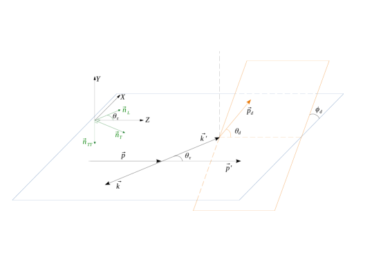
Figure 1: Kinematics in the $\tau\bar{\nu}_{\tau}$ CM reference system associated with Eq. (2), and used in Ref. Penalva et al. (2021b). The initial and final hadron three-momenta are $\vec{p}$ and $\vec{p}^{\,\prime}$, respectively, with $\vec{q}=\vec{p}-\vec{p}^{\,\prime}=\vec{0}$, while $\vec{k}^{\,\prime}$ and $\vec{k}$ are those of the intermediate $\tau$ and outgoing $\bar{\nu}_{\tau}$ emerging from the primary CC transition ($\vec{q}=\vec{k}+\vec{k}^{\,\prime}=\vec{0}$ ). In addition, $\vec{p}_{d}$ is the momentum of the tau-decay massive product ($\mu,\pi$ or $\rho$). We also show the unit vectors ($\vec{n}_{L},\vec{n}_{T}$ and $\vec{n}_{TT}$) which define the three independent projections of the $\tau-$polarization vector (see Ref. Penalva et al. (2021a)).

Finally, the $F^{d}_{012}(\omega,\xi_{d})$ two dimensional functions can be written as

$$F^{d}_{0}(\omega,\xi_{d}) = C_{n}^{d}(\omega,\xi_{d})+C_{P_{L}}^{d}(\omega,\xi_{d})\,\langle P^{\rm CM}_{L}\rangle(\omega),$$

$$F^{d}_{1}(\omega,\xi_{d}) = C_{A_{FB}}^{d}(\omega,\xi_{d})A_{FB}(\omega)+C_{Z_{L}}^{d}(\omega,\xi_{d})Z_{L}(\omega)+C_{P_{T}}^{d}(\omega,\xi_{d})\,\langle P^{\rm CM}_{T}\rangle(\omega),$$

$$F^{d}_{2}(\omega,\xi_{d}) = C_{A_{Q}}^{d}(\omega,\xi_{d})A_{Q}(\omega)+C_{Z_{Q}}^{d}(\omega,\xi_{d})Z_{Q}(\omega)+C_{Z_{\perp}}^{d}(\omega,\xi_{d})Z_{\perp}(\omega).$$ (4)

where the $C^{d}_{a}(\omega,\xi_{d})$ are kinematical coefficients that depend on the tau-decay mode. Their analytical expressions can be found, for the $\pi\nu_{\tau},\rho\nu_{\tau}$ and $\ell\bar{\nu}_{\ell}\nu_{\tau}$ cases, in Appendix G of Ref. Penalva et al. (2021b). In the leptonic mode we have kept effects due to the finite mass of the outgoing muon/electron, although making $m_{\ell}=0$ in those expressions should be a very good approximation, since both $m_{e},/m_{\tau}$ and $m_{\mu}/m_{\tau}$ are much smaller than one. The rest of the quantities in Eq. (4) are the tau-spin ($\langle P^{\rm CM}_{L,T}\rangle(\omega)$), tau-angular ($A_{FB,Q}(\omega)$) and tau-angular-spin ($Z_{L,Q,\perp}(\omega)$) asymmetries of the $H_{b}\to H_{c}\tau\bar{\nu}_{\tau}$ decay. Actually, these asymmetries and $d\Gamma_{\rm SL}/d\omega$ provide the maximal information that can be extracted from the study of polarized $H_{b}\to H_{c}\tau\bar{\nu}_{\tau}$ transitions, without considering CP non-conserving contributions Penalva et al. (2021a, b) (see Eq. (3.46) of the latter of these two references and the related discussion).

In Ref. Penalva et al. (2021b), we numerically analyzed the role that each of the observables, $d\Gamma_{\rm SL}/d\omega$, $\langle P^{\rm CM}_{L,T}\rangle(\omega)$, $A_{FB,Q}(\omega)$ and $Z_{L,Q,\perp}(\omega)$ could play to establish the existence of NP beyond the SM in $\Lambda_{b}\to\Lambda_{c}\tau\bar{\nu}_{\tau}$ semileptonic decays. In fact in that work, we obtained their general expressions, valid for any $H_{b}\to H_{c}\tau\bar{\nu}_{\tau}$ decay, when considering an extension of the SM comprising the full set of dimension-6 semileptonic $b\to c$ operators with left- and right-handed neutrinos. The effective low-energy Hamiltonian for that case is given by Mandal et al. (2020)

$$H_{\rm eff} = \frac{4G_{F}V_{cb}}{\sqrt{2}}\left[(1+C^{V}_{LL}){\cal O}^{V}_{LL}+C^{V}_{RL}{\cal O}^{V}_{RL}+C^{S}_{LL}{\cal O}^{S}_{LL}+C^{S}_{RL}{\cal O}^{S}_{RL}+C^{T}_{LL}{\cal O}^{T}_{LL}\right.$$ (5)

$$+ \left.C^{V}_{LR}{\cal O}^{V}_{LR}+C^{V}_{RR}{\cal O}^{V}_{RR}+C^{S}_{LR}{\cal O}^{S}_{LR}+C^{S}_{RR}{\cal O}^{S}_{RR}+C^{T}_{RR}{\cal O}^{T}_{RR}\right]+h.c.,$$

with left-handed neutrino fermionic operators given by

$${\cal O}^{V}_{(L,R)L}=(\bar{c}\gamma^{\mu}b_{L,R})(\bar{\ell}\gamma_{\mu}\nu_{\ell L}),\,{\cal O}^{S}_{(L,R)L}=(\bar{c}\,b_{L,R})(\bar{\ell}\,\nu_{\ell L}),\,{\cal O}^{T}_{LL}=(\bar{c}\,\sigma^{\mu\nu}b_{L})(\bar{\ell}\sigma_{\mu\nu}\nu_{\ell L})$$ (6)

and the right-handed neutrino ones

$${\cal O}^{V}_{(L,R)R}=(\bar{c}\gamma^{\mu}b_{L,R})(\bar{\ell}\gamma_{\mu}\nu_{\ell R}),\,{\cal O}^{S}_{(L,R)R}=(\bar{c}\,b_{L,R})(\bar{\ell}\,\nu_{\ell R}),\,{\cal O}^{T}_{RR}=(\bar{c}\,\sigma^{\mu\nu}b_{R})(\bar{\ell}\sigma_{\mu\nu}\nu_{\ell R}),$$ (7)

and where $\psi_{R,L}=(1\pm\gamma_{5})\psi/2$, $G_{F}=1.166\times 10^{-5}$ GeV^-2 and $V_{cb}$ is the corresponding Cabibbo-Kobayashi-Maskawa matrix element.

The asymmetries introduced in Eq. (4) depend on the pure hadronic structure functions and ten (complex) Wilson coefficients $C^{X}_{AB}$ ($X=S,V,T$ and $A,B=L,R$), which parameterize the possible deviations from the SM. The former depend on the form factors that parameterize the hadronic current and we have obtained them for $1/2^{+}\to 1/2^{+}$ Penalva et al. (2020b) and $0^{-}\to 0^{-},1^{-}$ Penalva et al. (2020a) decays.

The $d^{3}\Gamma_{d}/(d\omega d\xi_{d}d\cos\theta_{d})$ distribution, together with the combined analysis of its $(\xi_{d},\cos\theta_{d}$) dependence, gives access to all the above asymmetries as functions of $\omega$. The feasibility of such studies can be severely limited, however, by the statistical precision in the measurement of the triple differential decay width. Statistics can be increased by integrating in the $\cos\theta_{d}$ or/and $\xi_{d}$ variables, although in this case not all observables can be extracted. Thus, it is well known Tanaka and Watanabe (2010) that the distribution obtained after accumulating in the polar angle,

$$\frac{d^{2}\Gamma_{d}}{d\omega d\xi_{d}} = 2{\cal B}_{d}\frac{d\Gamma_{\rm SL}}{d\omega}\Big{\{}C_{n}^{d}(\omega,\xi_{d})+C_{P_{L}}^{d}(\omega,\xi_{d})\,\langle P^{\rm CM}_{L}\rangle(\omega)\Big{\}},$$ (8)

allows to determine $d\Gamma_{\rm SL}/d\omega$ and the CM $\tau$ longitudinal polarization [$\langle P^{\rm CM}_{L}\rangle(\omega)]$ since the, transition dependent, $C_{n}^{d}(\omega,\xi_{d})$ and $C_{P_{L}}^{d}(\omega,\xi_{d})$ coefficients are known kinematical factors Penalva et al. (2021b) (see also Alonso et al. (2017b); Tanaka and Watanabe (2010)). The averaged CM tau longitudinal polarization asymmetry,

$$P_{\tau}=-\frac{1}{\Gamma_{\rm SL}}\int d\omega\frac{d\Gamma_{\rm SL}}{d\omega}\langle P^{\rm CM}_{L}\rangle(\omega)$$ (9)

measured by Belle Hirose et al. (2017) for the $\bar{B}\to D^{*}\tau\bar{\nu}_{\tau}$ decay, immediately follows.

In Refs. Penalva et al. (2021a, b) we presented results for $\langle P^{\rm CM}_{L}\rangle(\omega)$ in the $\Lambda_{b}\to\Lambda_{c}\tau\bar{\nu}_{\tau}$ and $\bar{B}\to D^{(*)}\tau\bar{\nu}_{\tau}$ decays evaluated within the SM and different NP extensions. We also provided similar comparisons for $d\Gamma_{\rm SL}/d\omega$ in the $\Lambda_{b}\to\Lambda_{c}$ and $\bar{B}\to D^{(*)}$ and $\bar{B}_{c}\to J/\psi,\eta_{c}$ reactions in Refs. Penalva et al. (2019, 2020b) and Penalva et al. (2020a), respectively.

In this work, we take advantage of the analytical results derived in Penalva et al. (2021b), and we study, in secs.  II, III and IV, respectively, the alternative distributions $d^{2}\Gamma_{d}/(d\omega d\cos\theta_{d})$, $d\Gamma_{d}/d\cos\theta_{d}$ and $d\Gamma_{d}/dE_{d}$, which could also be measured in the near future with certain precision. We pay attention to the deviations with respect to the predictions of the SM for these new observables, considering NP operators constructed using both right- and left-handed neutrino fields, within the effective theory approach established by Eqs. (5)–(7). We will present results for the $\Lambda_{b}\to\Lambda_{c}\tau\,(\mu\bar{\nu}_{\mu}\nu_{\tau},\pi\nu_{\tau},\rho\nu_{\tau})\bar{\nu}_{\tau}$ (main text) and the $\bar{B}\to D^{(*)}\tau\,(\mu\bar{\nu}_{\mu}\nu_{\tau},\pi\nu_{\tau},\rho\nu_{\tau})\bar{\nu}_{\tau}$ sequential decays (Appendix B), obtained within different beyond the SM scenarios, and we discuss their use to extract some of the tau asymmetries introduced in Eq. (4). Details on the used form-factors and references to the original works where they were calculated can be found in Penalva et al. (2021a, b).

II The $d^{2}\Gamma/(d\omega d\cos\theta_{d})$ distribution

The limits on the $\xi_{d}$ variable are tau-decay mode dependent and thus, one has Penalva et al. (2021b)

$$\tau\to\mu\bar{\nu}_{\mu}\nu_{\tau} \Rightarrow y/\gamma\leq\xi_{d}\leq\xi_{2},$$

$$\tau\to(\pi,\rho)\nu_{\tau} \Rightarrow \frac{1-\beta}{2}+\frac{1+\beta}{2}y^{2}=\xi_{1}\leq\xi_{d}\leq\xi_{2}=\frac{1+\beta}{2}+\frac{1-\beta}{2}y^{2},$$ (10)

with $y=m_{d}/m_{\tau}$ and $m_{d}$ the mass of the tau-decay massive product ($\pi,\,\rho$ or $\mu$). After integration one obtains the double differential decay width

$$\frac{d^{2}\Gamma_{d}}{d\omega d\cos\theta_{d}} = {\cal B}_{d}\frac{d\Gamma_{\rm SL}}{d\omega}\Big{[}\widetilde{F}^{d}_{0}(\omega)+\widetilde{F}^{d}_{1}(\omega)\cos\theta_{d}+\widetilde{F}^{d}_{2}(\omega)P_{2}(\cos\theta_{d})\Big{]},$$ (11)

where the new angular expansion coefficients $\widetilde{F}^{d}_{{0,1,2}}(\omega)$ correspond to

$$\widetilde{F}^{d=\pi,\rho}_{{0,1,2}}(\omega)=\int_{\xi_{1}}^{\xi_{2}}F^{d}_{0,1,2}(\omega,\xi_{d})\,d\xi_{d},\qquad\widetilde{F}^{d=\ell\bar{\nu}_{\ell}}_{{0,1,2}}(\omega)=\int_{y/\gamma}^{\xi_{2}}F^{d=\ell\bar{\nu}_{\ell}}_{0,1,2}(\omega,\xi_{d})\,d\xi_{d}$$ (12)

and they can be extracted from the angular analysis of the statistically enhanced $d^{2}\Gamma/(d\omega d\cos\theta_{d})$ distribution. The overall normalization is recovered since $\widetilde{F}^{d}_{0}(\omega)=1/2$ for all tau-decay modes, and a further integration in the polar angle $\theta_{d}$ provides $d\Gamma_{d}/d\omega={\cal B}_{d}\ d\Gamma_{\rm SL}/d\omega$, which in this way can be experimentally obtained from the tau decay-chain reaction.

In what follows, we will focus on the non-trivial $\widetilde{F}^{d}_{1}(\omega)$ and $\widetilde{F}^{d}_{2}(\omega)$ functions, which read

$$\widetilde{F}^{d}_{1}(\omega) = C^{d}_{A_{FB}}(\omega)\,A_{FB}(\omega)+C^{d}_{Z_{L}}(\omega)\,Z_{L}(\omega)+C^{d}_{P_{T}}(\omega)\,\langle P_{T}^{\rm CM}\rangle(\omega),$$ (13)

$$\widetilde{F}^{d}_{2}(\omega) = C^{d}_{A_{Q}}(\omega)\,A_{Q}(\omega)+C^{d}_{Z_{Q}}(\omega)\,Z_{Q}(\omega)+C^{d}_{Z_{\perp}}(\omega)\,Z_{\perp}(\omega).$$ (14)

While the $\xi_{d}$ integration which gives rise to $\widetilde{F}_{0}^{d}(\omega)$ loses information on $\langle P^{\rm CM}_{L}\rangle(\omega)$, the statistically enhanced observables $\widetilde{F}_{1,2}^{\mu\bar{\nu}_{\mu}}(\omega)$ retain all the information on the other six asymmetries.

II.1 Tau-decay lepton mode

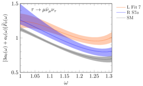
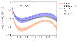
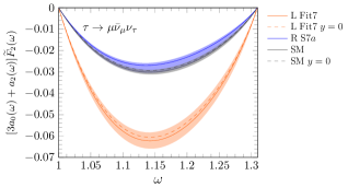
Figure 2: Results for the functions $[3a_{0}(\omega)+a_{2}(\omega)]\widetilde{F}^{\mu\bar{\nu}_{\mu}}_{0,1,2}(\omega)$ evaluated for the $\Lambda_{b}\to\Lambda_{c}\tau(\mu\bar{\nu}_{\mu}\nu_{\tau})\bar{\nu}_{\tau}$ decay, keeping the muon mass finite, and obtained from the SM and the NP models corresponding to Fit 7 of Ref Murgui et al. (2019) and Fit 7a of Ref Mandal et al. (2020). Error bands account for uncertainties induced by both form-factors and fitted Wilson coefficients (added in quadrature). In the SM and Fit 7 cases, we also display the results obtained neglecting the muon mass, as in Eqs. (15)-(17).

We start with the $\tau\to\mu\bar{\nu}_{\mu}\nu_{\tau}$ channel, since a measurement of the ratio of branching fractions ${\cal B}(\Lambda_{b}\to\Lambda_{c}\tau(\mu\nu_{\tau}\bar{\nu}_{\mu})\bar{\nu}_{\tau})/{\cal B}(\Lambda_{b}\to\Lambda_{c}\mu\bar{\nu}_{\mu})$ is in progress at the LHCb experiment. Moreover, as argued in the introduction, it would be very important to confront the recent LHCb measurement of ${\cal R}_{\Lambda_{c}}$, reconstructed using the three-prong hadronic $\tau$ decay, with results obtained when the tau lepton is identified from its leptonic decay into a muon. In the $y=m_{\mu}/m_{\tau}=0$ limit, which is a very good approximation (${\cal O}(y^{2})\sim$ 1%) in this case, and it is much better for the electron tau-decay mode, we find that the coefficient-functions, $C^{\mu\bar{\nu}_{\mu}}_{a}(\omega)$, are given by

$$C^{\mu\bar{\nu}_{\mu}}_{A_{FB}}(\omega)\Big{|}_{y=0} = \frac{3\pi\gamma\beta}{2}C^{\mu\bar{\nu}_{\mu}}_{P_{T}}(\omega)\Big{|}_{y=0}=\frac{1}{\beta^{2}}\Big{[}\beta-\frac{\operatorname{artanh}\beta}{\gamma^{2}}\Big{]},$$ (15)

$$C^{\mu\bar{\nu}_{\mu}}_{A_{Q}}(\omega)\Big{|}_{y=0} = -2\beta\gamma C^{\mu\bar{\nu}_{\mu}}_{Z_{\perp}}(\omega)\Big{|}_{y=0}=-\frac{1}{\beta^{3}}\Big{[}2\beta^{3}-3\beta+3\frac{\operatorname{artanh}\beta}{\gamma^{2}}\Big{]},$$ (16)

$$C^{\mu\bar{\nu}_{\mu}}_{Z_{L}}(\omega)\Big{|}_{y=0} = \frac{1}{3\gamma^{2}\beta^{3}}\Big{[}\beta-\operatorname{artanh}\beta\Big{]},\quad C^{\mu\bar{\nu}_{\mu}}_{Z_{Q}}(\omega)\Big{|}_{y=0}=\frac{1}{2\gamma^{2}\beta^{4}}\Big{[}3\beta-\big{(}3-\beta^{2}\big{)}\operatorname{artanh}\beta\Big{]},\$$ (17)

with $\operatorname{artanh}\beta=\ln\sqrt{\big{(}1+\beta\big{)}/\big{(}1-\beta\big{)}}$.

Here, we will present results for $\widetilde{F}^{\mu\bar{\nu}_{\mu}}_{0,1,2}(\omega)$ multiplied by the factor $n_{0}(\omega)$. For $\widetilde{F}^{\mu\bar{\nu}_{\mu}}_{0}(\omega)$ this amounts to represent $n_{0}(\omega)/2$ and, since this is the same for all tau-decay modes, it will only be shown for the muon tau-decay mode. As mentioned, the $n_{0}(\omega)$ function, introduced in Eq. (3), contains all the dynamical effects included in the $d\Gamma_{\rm SL}/d\omega$ differential semileptonic decay width, which appears as an overall normalization of the $d^{2}\Gamma/(d\omega d\cos\theta_{d})$ distribution. By showing $\widetilde{F}^{\mu\bar{\nu}_{\mu}}_{0,1,2}(\omega)$ times $n_{0}(\omega)$, we access to all the effects of possible NP beyond the SM on the tau production.

The $n_{0}(\omega)\widetilde{F}^{\mu\bar{\nu}_{\mu}}_{0,1,2}(\omega)$ functions, for the baryon $\Lambda_{b}\to\Lambda_{c}\tau(\mu\bar{\nu}_{\mu}\nu_{\tau})\bar{\nu}_{\tau}$ reaction, are displayed in Fig. 2. They have been evaluated within the SM and the beyond the SM scenarios of Fit 7 (7a) of Ref Murgui et al. (2019) (Mandal et al. (2020)), which only includes left- (right-)handed neutrino NP operators. These two NP scenarios have been adjusted to reproduce the anomalies observed in the LFU ${\cal R}_{D}$ and ${\cal R}_{D^{*}}$ ratios in $\bar{B}-$meson decays. However, in all cases, we see the results from Fit 7 of Ref Murgui et al. (2019) can be distinguished clearly from SM and Fit 7a model (R S7$a$ in the plots) ones. The results for the Fit 7a model are closer to the SM and in the case of the $\widetilde{F}^{\mu\bar{\nu}_{\mu}}_{1,2}(\omega)$ functions the uncertainty bands overlap in the whole $\omega$ interval. This is a reflection of what is obtained for the tau-asymmetries themselves, as can be seen in Fig.2 of Ref. Penalva et al. (2021b).

It is also very instructive to compare the full results for $n_{0}(\omega)\widetilde{F}^{\mu\bar{\nu}_{\mu}}_{1,2}(\omega)$ with those evaluated setting $A_{FB}(\omega)$ and $A_{Q}(\omega)$ to zero. This comparison is presented in Fig. 3. What can be inferred from this comparison is that the contribution of the spin ($\langle P^{\rm CM}_{T}\rangle(\omega)$) and angular-spin ($Z_{L,\,Q,\,\perp}(\omega)$) asymmetry terms are sizable and dominant in most of the $\omega$ interval. This is clearly the case in the vicinity of the end-point of the distributions, $q^{2}=m_{\tau}^{2}$ ($\beta=0$). In fact, using Eqs. (15)-(17), we find in the $y\to 0$ limit

$$\widetilde{F}^{\mu\bar{\nu}_{\mu}}_{1}(\omega) \sim \frac{1}{9\pi}\Big{[}4\langle P_{T}^{\rm CM}\rangle(\omega_{\rm max})-\pi Z_{L}(\omega_{\rm max})\Big{]}+\frac{\beta}{9}\Big{[}6A_{FB}(\omega_{\rm max})$$ (18)

$$-\frac{m^{2}_{\tau}}{\pi MM^{\prime}}\big{[}4\langle P_{T}^{\rm CM}\rangle^{\prime}(\omega_{\rm max})-\pi Z_{L}^{\prime}(\omega_{\rm max})\big{]}\Big{]}+{\cal O}(\beta^{2}),$$

$$\widetilde{F}^{\mu\bar{\nu}_{\mu}}_{2}(\omega) \sim -\frac{\beta}{15}\Big{[}3Z_{\perp}(\omega_{\rm max})+2Z_{Q}(\omega_{\rm max})\Big{]}+\frac{\beta^{2}}{15}\Big{[}6A_{Q}(\omega_{\rm max})$$ (19)

$$+\frac{m^{2}_{\tau}}{MM^{\prime}}\big{[}3Z^{\prime}_{\perp}(\omega_{\rm max})+2Z^{\prime}_{Q}(\omega_{\rm max})\big{]}\Big{]}+{\cal O}(\beta^{3}),$$

with $\omega_{\rm max}=\omega(q^{2}=m^{2}_{\tau})=(M^{2}+M^{\prime 2}-m^{2}_{\tau})/(2MM^{\prime})$, which show that the contributions of the tau-angular asymmetries $A_{FB}$ and $A_{Q}$ are suppressed by a factor $\beta$ with respect to those proportional to $\langle P_{T}^{\rm CM}\rangle$ and $Z_{L,Q,\perp}$.

Thus, these two $\widetilde{F}^{\mu\bar{\nu}_{\mu}}_{1,2}(\omega)$ observables, which have an increased statistics over $F^{\mu\bar{\nu}_{\mu}}_{1,2}(\omega,\xi_{d})$, could be ideal to measure tau-spin related asymmetries other than the commonly reported $\langle P_{L}^{\rm CM}\rangle(\omega)$, extracted from the $d^{2}\Gamma_{d}/(d\omega dE_{d})$ distribution.

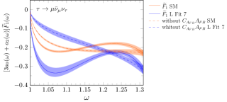
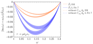
Figure 3: Comparison of the full results (solid lines) for $[3a_{0}(\omega)+a_{2}(\omega)]\widetilde{F}^{\mu\bar{\nu}_{\mu}}_{1,2}(\omega)$ with those obtained setting $A_{FB}(\omega)$ and $A_{Q}(\omega)$ to zero (dashed lines). The muon mass is kept finite. The results have been obtained for the $\Lambda_{b}\to\Lambda_{c}\tau(\mu\bar{\nu}_{\mu}\nu_{\tau})\bar{\nu}_{\tau}$ sequential decay, within the SM and the NP model corresponding to Fit 7 of Ref Murgui et al. (2019).

II.2 Tau-decay hadron modes

The behavior seen in Fig. 3 of the previous section for the muon is enhanced in the pion decay mode. After performing the integration over the variable $\xi_{d}$, we have that, neglecting $y^{2}$ ($m^{2}_{\mu}/m^{2}_{\tau}$ and $m_{\pi}^{2}/m_{\tau}^{2}$) corrections, the coefficients multiplying the two angular asymmetries $A_{FB,\,Q}(\omega)$ are the same as in the leptonic mode, while for the rest of the spin and angular-spin asymmetries there is an extra factor of $-3$. This is to say

$$C^{\pi}_{A_{FB},A_{Q}}(\omega)=C^{\mu\bar{\nu}_{\mu}}_{A_{FB},A_{Q}}(\omega)+{\cal O}(y^{2}),\quad C^{\pi}_{P_{T},Z_{L},Z_{Q},Z_{\perp}}(\omega)=-3\,C^{\mu\bar{\nu}_{\mu}}_{P_{T},Z_{L},Z_{Q},Z_{\perp}}(\omega)+{\cal O}(y^{2})$$ (20)

This difference in the spin analyzing power makes the pion tau-decay mode a better candidate for the extraction of information on the spin and angular-spin asymmetries. Exact expressions, without the $y=0$ approximation, for the $\pi$ and $\rho$ decay modes are given in Appendix A, although neglecting $m_{\pi}^{2}/m_{\tau}^{2}$ contributions is again an excellent approximation for the pion case. For the $\rho$ decay mode, the spin analyzing power is suppressed, with respect to the pion case, by the factor $a_{\rho}=(m_{\tau}^{2}-2m_{\rho}^{2})/(m_{\tau}^{2}+2m_{\rho}^{2})\approx 0.45$ (see Appendix A), although it is still greater than for the lepton decay mode.

Full results, as well as results obtained setting the angular $A_{FB,\,Q}(\omega)$ asymmetry terms to zero, for the hadron-mode $\widetilde{F}^{\pi,\rho}_{1,2}(\omega)$ functions are shown in Fig. 4 for the $\Lambda_{b}\to\Lambda_{c}\tau(\pi\nu_{\tau},\,\rho\nu_{\tau})\bar{\nu}_{\tau}$ decays, accounting for all mass term corrections ($y=m_{\pi,\,\rho}/m_{\tau}\neq 0$). As expected, we see that the hadron modes, in particular the pion one, show a great sensitivity to the spin-angular asymmetries, which could be extracted from $\widetilde{F}^{\pi,\rho}_{1}(\omega)$ and $\widetilde{F}^{\pi,\rho}_{2}(\omega)$. These new observables are independent of the $d\Gamma_{\rm SL}/d\omega$ and $\langle P^{\rm CM}_{L}\rangle(\omega)$ distributions Penalva et al. (2021a, b), and they will provide new constraints on the physics governing the $\Lambda_{b}\to\Lambda_{c}\tau\bar{\nu}_{\tau}$ parent decay.

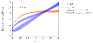
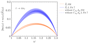
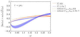
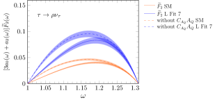
Figure 4: Same as Fig. 3, but for the $[3a_{0}(\omega)+a_{2}(\omega)]\widetilde{F}^{\pi,\,\rho}_{1,2}(\omega)$ hadron-mode distributions. We use the expressions for the coefficients collected in Appendix A, which were obtained keeping the pion and rho meson masses finite.

The $\Lambda_{b}\to\Lambda_{c}\tau(\pi\nu_{\tau},\rho\nu_{\tau})\bar{\nu}_{\tau}$ reaction channels have a lower reconstruction efficiency at LHCb than the one driven by the $\tau$-decay lepton mode Mar . However, they might be accessible in the future, or be easier to reconstruct in other machines and/or chains initiated by other parent semileptonic decays. For that reason, in Appendix B we also present results for distributions obtained from the sequential $\bar{B}\to D^{(*)}\tau(\pi\nu_{\tau},\rho\nu_{\tau})\bar{\nu}_{\tau}$ decays.

III The $d\Gamma/d\cos\theta_{d}$ distribution

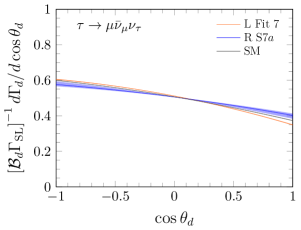
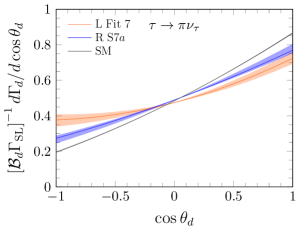
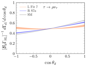
Figure 5: Angular $d\Gamma/d\cos\theta_{d}$ distribution for the $\Lambda_{b}\to\Lambda_{c}\tau(\mu\bar{\nu}_{\mu}\nu_{\tau},\,\pi\nu_{\tau},\,\rho\nu_{\tau})\bar{\nu}_{\tau}$ decays, keeping $y=m_{d}/m_{\tau}$ to its finite value, and obtained within the SM and the beyond the SM scenarios of Fit 7 (7a) of Ref Murgui et al. (2019) (Mandal et al. (2020)), which only includes left- (right-)handed neutrino NP operators. Error bands account for uncertainties induced by both form-factors and fitted Wilson coefficients (added in quadrature).

A further integration in $\omega$ additionally enhances the statistics. Although it prevents a separate determination of each of the asymmetries, it is still a useful observable in the search for NP beyond the SM. This angular distribution reads

$$\frac{d\Gamma_{d}}{d\cos\theta_{d}}={\cal B}_{d}\Gamma_{\rm SL}\Big{[}\frac{1}{2}+\widehat{F}_{1}^{d}\cos\theta_{d}+\widehat{F}_{2}^{d}\,P_{2}(\cos\theta_{d})\Big{]},\quad\widehat{F}_{1,2}^{d}=\frac{1}{\Gamma}_{\rm SL}\int_{1}^{\omega_{\rm max}}\frac{d\Gamma_{\rm SL}}{d\omega}\widetilde{F}_{1,2}^{d}(\omega)\,d\omega.$$ (21)

and an appropriate angular analysis of $d\Gamma/d\cos\theta_{d}$ should allow to determine the total semileptonic width $\Gamma_{\rm SL}$ and the moments $\widehat{F}_{1}^{d}$ and $\widehat{F}_{2}^{d}$.

The full distributions of Eq. (21), normalized by ${\cal B}_{d}\Gamma_{\rm SL}$, for the $\Lambda_{b}\to\Lambda_{c}\tau(\mu\bar{\nu}_{\mu}\nu_{\tau},\pi\nu_{\tau},\rho\nu_{\tau})\bar{\nu}_{\tau}$ chain-decays, evaluated for the SM and different NP models are presented in Fig. 5. The integrated width $\Gamma_{\rm SL}$ and the angular moments $\widehat{F}_{1}^{d}$ and $\widehat{F}_{2}^{d}$ obtained from, each of the physics scenarios considered in the figure are collected in Tables 1 and 2, respectively. As already mentioned, all NP scenarios have been adjusted to reproduce the anomalies observed in the ${\cal R}_{D}$ and ${\cal R}_{D^{*}}$ ratios in $\bar{B}-$meson decays, and they all predict values for ${\cal R}_{\Lambda_{c}}$ that are at variance ($2\sigma-3\sigma$) with both the SM prediction and the recent LHCb measurement, the latter two being within $1\sigma$. In addition, we also observe differences in $\widehat{F}_{1}^{d}$ and $\widehat{F}_{2}^{d}$, that are hardly accounted for by errors. This situation is reflected in Fig. 5, where we see that the best discriminating power between the SM and different NP extensions is reached for forward and backward emission in the $\tau$-hadron decay modes, which are more sensitive to $\widehat{F}_{1}^{\pi,\rho}$ and $\widehat{F}_{2}^{\pi,\rho}$. In fact, these new observables are shown as excellent tools to discern between different inputs for the semileptonic $\Lambda_{b}\to\Lambda_{c}\tau\bar{\nu}_{\tau}$ parent reaction.

In Appendix B we collect the corresponding results for the sequential $\bar{B}\to D^{(*)}\tau(\mu\bar{\nu}_{\mu}\nu_{\tau},\pi\nu_{\tau},\rho\nu_{\tau})\bar{\nu}_{\tau}$ decays.

	SM	L Fit 7 Murgui et al. (2019)	R S7a Mandal et al. (2020)	LHCb Aaij et al. (2022)
$\Gamma_{e(\mu)}$	$2.15\pm 0.08$
$\Gamma_{\tau}$	$0.715\pm 0.015$	$0.89\pm 0.05$	$0.81\pm 0.06$
${\cal R}_{\Lambda_{c}}$	$0.332\pm 0.007$	$0.41\pm 0.02$	$0.38\pm 0.03$	$0.242\pm 0.026\pm 0.040\pm 0.059$

Table 1: Semileptonic decay widths $\Gamma_{\tau}=\Gamma\left(\Lambda_{b}\to\Lambda_{c}\tau\bar{\nu}_{\tau}\right)$ and $\Gamma_{e(\mu)}=\Gamma\left(\Lambda_{b}\to\Lambda_{c}\,e(\mu)\bar{\nu}_{e(\mu)}\right)$ [units of $\left(10\times|V_{cb}|^{2}{\rm ps}^{-1}\right)$] and ratios ${\cal R}_{\Lambda_{c}}=\Gamma\left(\Lambda_{b}\to\Lambda_{c}\tau\bar{\nu}_{\tau}\right)/\Gamma\left(\Lambda_{b}\to\Lambda_{c}\,e(\mu)\bar{\nu}_{e(\mu)}\right)$ obtained in the SM, the NP model Fit 7 (7a) of Ref Murgui et al. (2019) (Mandal et al. (2020)), which only includes left- (right-)handed neutrino NP operators. Errors induced by the uncertainties in the form-factors and Wilson Coefficients are added in quadrature. The recent LHCb Aaij et al. (2022) measurement of the ${\cal R}_{\Lambda_{c}}$ ratio, with the tau being reconstructed using the $\tau\to\pi^{-}\pi^{+}\pi^{-}(\pi^{0})\,\nu_{\tau}$ decay, is also shown.

	$\widehat{F}_{1}^{\mu\bar{\nu}_{\mu}}$	$\widehat{F}_{2}^{\mu\bar{\nu}_{\mu}}$	$\widehat{F}_{1}^{\pi}$	$\widehat{F}_{2}^{\pi}$	$\widehat{F}_{1}^{\rho}$	$\widehat{F}_{2}^{\rho}$
SM	$-0.113\pm 0.001$	$-0.0137\pm 0.0003$	$0.336\pm 0.003$	$0.0306\pm 0.0007$	$0.141\pm 0.002$	$0.0166\pm 0.0004$
L Fit 7	$-0.128\pm 0.003$	$-0.0228\pm 0.0005$	$0.17\pm 0.03$	$0.0507\pm 0.0013$	$0.019^{+0.025}_{-0.020}$	$0.0275\pm 0.0007$
R S7a	$-0.087^{+0.010}_{-0.017}$	$-0.0108^{+0.0006}_{-0.0011}$	$0.25^{+0.03}_{-0.02}$	$0.023^{+0.002}_{-0.003}$	$0.101^{+0.017}_{-0.005}$	$0.0108^{+0.0027}_{-0.0008}$

Table 2: Predictions for the angular moments $\widehat{F}^{d}_{1,\,2}$ for the $\Lambda_{b}\to\Lambda_{c}\tau(\mu\bar{\nu}_{\mu}\nu_{\tau},\,\pi\nu_{\tau},\,\rho\nu_{\tau})\bar{\nu}_{\tau}$ decays evaluated in the SM and the same NP scenarios considered in Table 1.

IV The $d\Gamma/dE_{d}$ distribution

Finally in this section we study the energy ($E_{d}$) distribution of the charged (massive) product from the tau-decay. The idea is to increase the statistics by accumulating events for all allowed $\omega$ values and provide only the $E_{d}$ spectrum. Regardless detector efficiencies considerations, the $d\Gamma/dE_{d}$ differential decay width could be determined as precisely as $d\Gamma/d\cos\theta_{d}$ (discussed in Sec. III) or $d\Gamma_{\rm SL}/d\omega$, with the three distributions giving independent information about the dynamics governing the semileptonic $b\to c\tau\bar{\nu}_{\tau}$ transition Penalva et al. (2020b, 2021a). From the $d^{2}\Gamma_{d}/(d\omega d\xi_{d})$ differential decay width given in Eq. (8) and using $E_{d}=\gamma m_{\tau}\xi_{d}$, we have

$$\frac{d\Gamma_{d}}{dE_{d}} = 2{\cal B}_{d}\int_{\omega_{\rm inf}(E_{d})}^{\omega_{\rm sup}(E_{d})}d\omega\frac{1}{\gamma m_{\tau}}\frac{d\Gamma_{\rm SL}}{d\omega}\Big{\{}C_{n}^{d}(\omega,E_{d})+C_{P_{L}}^{d}(\omega,E_{d})\,\langle P^{\rm CM}_{L}\rangle(\omega)\Big{\}},$$ (22)

The maximum energy, $E_{d}^{\rm max}$, of the massive product from the tau-decay is

$$E_{d}^{\rm max}=\frac{(M-M^{\prime})^{2}+m_{d}^{2}}{2(M-M^{\prime})}$$ (23)

while the minimum one, $E_{d}^{\rm min}$, depends on the tau-decay mode and the order relation between $(M-M^{\prime})$ and $m_{\tau}^{2}/m_{d}$. For the reactions considered in this work, we have $(M-M^{\prime})\leq m_{\tau}^{2}/m_{d}$ and hence

$$E_{d}^{\rm min} = m_{d},\quad d=\mu\bar{\nu}_{\mu},e\bar{\nu}_{e}$$ (24)

$$E_{d}^{\rm min} = \frac{m_{d}^{2}(M-M^{\prime})^{2}+m_{\tau}^{4}}{2m_{\tau}^{2}(M-M^{\prime})},\quad d=\pi,\rho$$ (25)

while $E_{d}^{\rm min}=m_{d}$ for the hadronic case if $(M-M^{\prime})\geq m_{\tau}^{2}/m_{d}$. This latter situation occurs for instance in the sequential $\bar{B}\to\pi\tau(\rho\nu_{\tau})\bar{\nu}_{\tau}$ reaction, involving the CC $b\to u\tau\bar{\nu}_{\tau}$ transition.

To perform the $\omega$ integration, first we have to obtain the allowed variation of the $\omega$ variable for a given $E_{d}$, i.e., to determine $\omega_{\rm inf}(E_{d})$ and $\omega_{\rm sup}(E_{d})$ in Eq. (22). This requires to invert the limits in Eq. (10) and the result depends on the tau-decay channel

1. $\tau\to\mu\bar{\nu}_{\mu}\nu_{\tau}$ and $\tau\to e\bar{\nu}_{e}\nu_{\tau}$: In this case, $m_{d}$ is either the muon or the electron mass, and considering $(M-M^{\prime})\leq m_{\tau}^{2}/m_{d}$, we find $\omega_{\rm inf}(E_{d})=1$, while

   $$\omega_{\rm sup}(E_{d}) = \omega_{\rm max}=\frac{M^{2}+M^{\prime 2}-m^{2}_{\tau}}{2MM^{\prime}},\quad E_{d}\leq\frac{m_{\tau}^{2}+m_{d}^{2}}{2m_{\tau}}$$ (26)

   $$\omega_{\rm sup}(E_{d}) = \frac{M^{2}+M^{\prime 2}-\left(E_{d}+\sqrt{E_{d}^{2}-m_{d}^{2}}\,\right)^{2}}{2MM^{\prime}},\quad E_{d}\geq\frac{m_{\tau}^{2}+m_{d}^{2}}{2m_{\tau}}$$ (27)

2. $\tau\to\pi\nu_{\tau}$ and $\tau\to\rho\nu_{\tau}$: In this case $m_{d}$ is either the pion or rho mass, and considering $(M-M^{\prime})\leq m_{\tau}^{2}/m_{d}$, we also find $\omega_{\rm inf}(E_{d})=1$, while

   $$\omega_{\rm sup}(E_{d}) = \frac{M^{2}+M^{\prime 2}-m_{\tau}^{4}\left(E_{d}-\sqrt{E_{d}^{2}-m_{d}^{2}}\,\right)^{2}/m_{d}^{4}}{2MM^{\prime}},\quad E_{d}\leq\frac{m_{\tau}^{2}+m_{d}^{2}}{2m_{\tau}}$$ (28)

   $$\omega_{\rm sup}(E_{d}) = \frac{M^{2}+M^{\prime 2}-\left(E_{d}+\sqrt{E_{d}^{2}-m_{d}^{2}}\,\right)^{2}}{2MM^{\prime}},\quad E_{d}\geq\frac{m_{\tau}^{2}+m_{d}^{2}}{2m_{\tau}}$$ (29)

From the differential distribution of Eq. (22), we define a new dimensionless observable $\widehat{F}^{d}_{0}(E_{d})$, such that $d\Gamma/dE_{d}=2{\cal B}_{d}\Gamma_{\rm SL}\widehat{F}^{d}_{0}(E_{d})/m_{\tau}$, with $\Gamma_{\rm SL}$ the total $H_{b}\to H_{c}\tau\bar{\nu}_{\tau}$ semileptonic decay width, and

$$\widehat{F}^{d}_{0}(E_{d})=\frac{1}{\Gamma_{\rm SL}}\int_{1}^{\omega_{\rm sup}(E_{d})}\frac{1}{\gamma}\frac{d\Gamma_{\rm SL}}{d\omega}\Big{\{}C_{n}^{d}(\omega,E_{d})+C_{P_{L}}^{d}(\omega,E_{d})\,\langle P^{\rm CM}_{L}\rangle(\omega)\Big{\}}\,d\omega,$$ (30)

where the corresponding $\omega_{\rm sup}(E_{d})$ values can be read out from Eqs. (26)-(29). This energy function is normalized for all tau-decay channels to

$$\frac{1}{m_{\tau}}\int_{E_{d}^{\rm min}}^{E_{d}^{\rm min}}dE_{d}\widehat{F}^{d}_{0}(E_{d})=\frac{1}{m_{\tau}\Gamma_{\rm SL}}\int_{E_{d}^{\rm min}}^{E_{d}^{\rm min}}\int_{1}^{\omega_{\rm sup}(E_{d})}\frac{1}{\gamma}\frac{d\Gamma_{\rm SL}}{d\omega}C_{n}^{d}(\omega,E_{d})\,d\omega dE_{d}=\frac{1}{2}$$ (31)

Although the CM $\tau$ longitudinal polarization $\langle P^{\rm CM}_{L}\rangle(\omega)$ does not contribute to the normalization of $\widehat{F}^{d}_{0}(E_{d})$, it still affects the energy shape of the observable. This is in contrast to what happens if, instead, one accumulates on the variable $\xi_{d}$ in the $d^{2}\Gamma_{d}/(d\omega d\xi_{d})$ distribution of Eq. (8) to obtain $d\Gamma_{d}/d\omega$. As already mentioned, this $\xi_{d}$ (or equivalently $E_{d}$) integration removes permanently any information about $\langle P^{\rm CM}_{L}\rangle$.

The results for $\widehat{F}^{d}_{0}(E_{d})$ in the $\Lambda_{b}\to\Lambda_{c}\tau(\mu\bar{\nu}_{\mu}\nu_{\tau},\,\pi\nu_{\tau},\,\rho\nu_{\tau})\bar{\nu}_{\tau}$ decays are presented in Fig. 6. We observe small changes between the predictions obtained from the SM and any of the NP models considered in this work, pointing out to a little influence of the $\langle P^{\rm CM}_{L}\rangle$ contribution in this distribution. Nevertheless, for the hadron modes, we again see that Fit 7 of Ref Murgui et al. (2019) gives, in some regions, significantly different results from those obtained in the SM and Fit 7a, while the latter agrees with the SM within uncertainty bands.

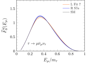
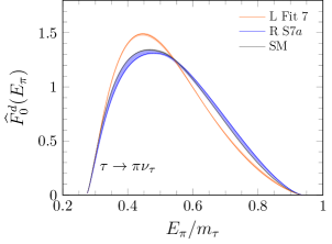
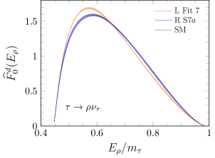
Figure 6: Predictions for the $\widehat{F}^{d}_{0}(E_{d})$ energy distribution [Eq. (30)] for the $\Lambda_{b}\to\Lambda_{c}\tau(\mu\bar{\nu}_{\mu}\nu_{\tau},\,\pi\nu_{\tau},\,\rho\nu_{\tau})\bar{\nu}_{\tau}$ decays, keeping $y=m_{d}/m_{\tau}$ finite, obtained within the SM and the NP scenarios corresponding to Fit 7 of Ref Murgui et al. (2019) and Fit 7a of Ref Mandal et al. (2020).

V Summary and conclusions

Using the analytical results derived in Penalva et al. (2021b), we have studied the $d^{2}\Gamma_{d}/(d\omega d\cos\theta_{d})$, $d\Gamma_{d}/d\cos\theta_{d}$ and $d\Gamma_{d}/dE_{d}$ distributions, which are defined in terms of the visible energy and polar angle of the charged particle from the $\tau$-decay in $b\to c\tau\,(\mu\bar{\nu}_{\mu}\nu_{\tau},\pi\nu_{\tau},\rho\nu_{\tau})\bar{\nu}_{\tau}$ reactions and that one expects to be measured at some point in the near future. The first two contain information on the CM transverse tau-spin ($\langle P^{\rm CM}_{T}\rangle(\omega)$), tau-angular ($A_{FB,Q}(\omega)$) and tau-angular-spin ($Z_{L,Q,\perp}(\omega)$) asymmetries of the $H_{b}\to H_{c}\tau\bar{\nu}_{\tau}$ parent decay. Hence, from the dynamical point of view, these observables are richer than the commonly used one, $d^{2}\Gamma_{d}/(d\omega dE_{d})$, since the latter gives access only to the CM tau longitudinal polarization $\langle P^{\rm CM}_{L}\rangle(\omega)$. We have paid attention to the deviations with respect to the predictions of the SM for these new observables, considering NP operators constructed using both left- and right-handed neutrino fields, within an effective theory approach. We have presented results for these distributions in $\Lambda_{b}\to\Lambda_{c}\tau\,(\mu\bar{\nu}_{\mu}\nu_{\tau},\pi\nu_{\tau},\rho\nu_{\tau})\bar{\nu}_{\tau}$ (main text) and $\bar{B}\to D^{(*)}\tau\,(\mu\bar{\nu}_{\mu}\nu_{\tau},\pi\nu_{\tau},\rho\nu_{\tau})\bar{\nu}_{\tau}$ (Appendix B) sequential decays, within different beyond the SM scenarios, and we have discussed their use to disentangle between different NP models. In this respect, we have seen that $d\Gamma_{d}/d\cos\theta_{d}$, if measured with sufficiently good statistics, becomes quite useful, especially in the $\tau\to\pi\nu_{\tau}$ decay mode.

The study carried out in this work acquires a special relevance due to the recent LHCb measurement of the LFU ratio ${\cal R}_{\Lambda_{c}}$ in agreement, within errors, with the SM prediction. The experiment identified the $\tau$ using the three-prong hadronic $\tau^{-}\to\pi^{-}\pi^{+}\pi^{-}(\pi^{0})\,\nu_{\tau}$ decay, and this result for ${\cal R}_{\Lambda_{c}}$, which is in conflict with the phenomenology from the $b$-meson sector, needs to be confirmed employing other reconstruction channels.

We are aware of the difficulties in measuring the accumulated distributions proposed in this work for the $\Lambda_{b}\to\Lambda_{c}\tau(\mu\bar{\nu}_{\mu}\nu_{\tau},\pi\nu_{\tau},\rho\nu_{\tau})\bar{\nu}_{\tau}$ decay at LHC Cerri et al. (2019). As mentioned in the Introduction, the LHCb collaboration is conducting a study on this reaction using the $\tau\to\mu\bar{\nu}_{\mu}\nu_{\tau}$ reconstruction channel. We expect that this would imply the measurement of some of the muon variables and thus the determination, in the not too distant future and with a certain accuracy, of some or all, of the differential decays widths analyzed in this work. If the presence of NP is confirmed, going beyond the pure measurement of $R(\Lambda_{c})$ (and other ratios) is essential to disentangle among different SM extensions. Furthermore, we have also predicted accumulated distributions for the $\bar{B}\to D^{(*)}$ semileptonic reactions, for which, within the context of the plan to increase luminosity at the LHC, the prospects look more favorable Cerri et al. (2019).

Appendix A Coefficients $C^{\pi,\,\rho}_{A_{FB,Q}}(\omega)$, $C^{\pi,\,\rho}_{P_{T}}(\omega)$ and $C^{\pi,\,\rho}_{Z_{L,Q,\perp}}(\omega)$ for the $\pi\nu_{\tau}$ and $\rho\nu_{\tau}$ $\tau$-decay modes

In this appendix, we give the coefficients which define the $\widetilde{F}_{12}^{\pi,\,\rho}(\omega)$ distributions in terms of the tau-asymmetries, through Eqs. (13) and  (14), for the $\pi\nu_{\tau}$ and $\rho\nu_{\tau}$ tau-decay modes keeping finite $y=m_{d}/m_{\tau}$. We use the analytical expressions derived in Ref. Penalva et al. (2021b) for the two dimensional $C^{\pi,\,\rho}_{A_{FB,Q}}(\omega,\xi_{d})$, $C^{\pi,\,\rho}_{P_{T}}(\omega,\xi_{d})$ and $C^{\pi,\,\rho}_{Z_{L,Q,\perp}}(\omega,\xi_{d})$ functions and integrate over the variable $\xi_{d}$. We first discuss the coefficient of the forward-backward asymmetry,

$$C^{\pi,\rho}_{A_{FB}}(\omega)=\left\{\begin{array}[]{c}\frac{1+y^{2}}{1-y^{2}}\frac{1}{\beta^{2}}\left[\beta-\frac{\operatorname{artanh}\beta}{\gamma^{2}}\right],\quad y^{2}\leq\frac{1-\beta}{1+\beta}=\frac{m^{2}_{\tau}}{q^{2}}\\ \\ \frac{1+y^{2}}{1-y^{2}}\frac{1}{\beta^{2}}\left[\frac{1-y^{2}}{1+y^{2}}+\frac{\log y}{\gamma^{2}}\right],\quad y^{2}\geq\frac{1-\beta}{1+\beta}=\frac{m^{2}_{\tau}}{q^{2}}\end{array}\right.$$ (32)

For the reactions studied in this work, we always have $y^{2}\leq m^{2}_{\tau}/q^{2}$ for all available $q^{2}$ values and thus, the first of the above possibilities should be taken. The situation is repeated for the rest of the coefficients. For brevity, we only give below the expressions for the $y^{2}<m^{2}_{\tau}/q^{2}$ case,

$$C^{\pi,\rho}_{Z_{L}}(\omega) = -a_{\pi,\rho}\left[\frac{1+4y^{2}+y^{4}}{\left(1-y^{2}\right)^{2}}\frac{1}{\gamma^{2}\beta^{3}}\left(\beta-\operatorname{artanh}\beta\right)+\frac{2y^{2}}{\left(1-y^{2}\right)^{2}}\right]$$ (33)

$$C^{\pi,\rho}_{P_{T}}(\omega) = -a_{\pi,\rho}\frac{2}{\pi\gamma\beta}\left[\frac{1+4y^{2}+y^{4}}{1-y^{4}}C^{\pi,\rho}_{A_{FB}}(\omega)-\frac{4y^{2}}{\left(1-y^{2}\right)^{2}}\operatorname{artanh}\beta\right]$$ (34)

$$C^{\pi,\rho}_{A_{Q}}(\omega) = \frac{1}{2\beta^{2}}\left[3-\beta^{2}+3\frac{1+\left(2+4\gamma^{2}\right)y^{2}+y^{4}}{2\gamma^{3}\beta y\left(1-y^{2}\right)}\operatorname{artanh}\Big{(}\frac{2\gamma\beta y}{1-y^{2}}\Big{)}\right]$$ (35)

$$-\frac{3}{\gamma^{2}\beta^{3}}\frac{1+y^{2}}{1-y^{2}}\operatorname{artanh}\Big{(}\frac{1+y^{2}}{1-y^{2}}\beta\Big{)}$$

$$C^{\pi,\rho}_{Z_{Q}}(\omega) = -3a_{\pi,\rho}\left[\frac{1+y^{2}}{\beta^{3}\gamma^{2}\left(1-y^{2}\right)}\left(1+\frac{1}{4\gamma\beta y}\frac{1+\left(10+4\gamma^{2}\right)y^{2}+y^{4}}{1-y^{2}}\operatorname{artanh}\Big{(}\frac{2\gamma\beta y}{1-y^{2}}\Big{)}\right)\right.$$ (36)

$$\left.-\frac{2\gamma^{2}\left(1+4y^{2}+y^{4}\right)+\left(1+y^{2}\right)^{2}}{2\gamma^{4}\beta^{4}\left(1-y^{2}\right)^{2}}\operatorname{artanh}\Big{(}\frac{1+y^{2}}{1-y^{2}}\beta\Big{)}\right]$$

$$C^{\pi,\rho}_{Z_{\perp}}(\omega) = \frac{3a_{\pi,\rho}}{2\beta^{4}\gamma}\frac{1}{\left(1-y^{2}\right)^{2}}\left[\left(2\beta-\beta^{3}\right)\left(1-y^{4}\right)-\frac{3\left(1+y^{2}\right)^{2}+4\gamma^{2}y^{2}}{\gamma^{2}}\operatorname{artanh}\Big{(}\frac{1+y^{2}}{1-y^{2}}\beta\Big{)}\right.$$ (37)

$$\left.+\frac{1+y^{2}}{2y}\,\frac{\left(1+y^{2}\right)^{2}+12\gamma^{2}y^{2}}{\gamma^{3}}\operatorname{artanh}\Big{(}\frac{2\gamma\beta y}{1-y^{2}}\Big{)}\right]$$

with $a_{\pi}=1$ and $a_{\rho}=(m^{2}_{\tau}-2m^{2}_{\rho})/(m^{2}_{\tau}+2m^{2}_{\rho})$. Note that all the arguments of the $\operatorname{artanh}$-functions are smaller than one, since the above expressions are only valid for $y^{2}<(1-\beta)/(1+\beta)$.

Appendix B Results for the $\bar{B}\to D^{(*)}\tau(\mu\bar{\nu}_{\mu}\nu_{\tau},\pi\nu_{\tau},\rho\nu_{\tau})\bar{\nu}_{\tau}$ sequential decays

		SM	L Fit 7 Murgui et al. (2019)	R S7a Mandal et al. (2020)	HFLAV Amhis et al. (2021)
	$\Gamma_{e(\mu)}$	$0.87\pm 0.03$
$\bar{B}\to D$	$\Gamma_{\tau}$	$0.262\pm 0.005$	$0.34\pm 0.04$	$0.292^{+0.060}_{-0.014}$
	${\cal R}_{D}$	$0.300^{+0.005}_{-0.004}$	$0.388^{+0.044}_{-0.045}$	$0.334^{+0.070}_{-0.015}$	$0.340\pm 0.027\pm 0.013$
	$\Gamma_{e(\mu)}$	$2.01^{+0.07}_{-0.08}$
$\bar{B}\to D^{*}$	$\Gamma_{\tau}$	$0.512^{+0.013}_{-0.014}$	$0.61\pm 0.03$	$0.59\pm 0.03$
	${\cal R}_{D^{*}}$	$0.255\pm 0.003$	$0.306\pm 0.013$	$0.292^{+0.014}_{-0.015}$	$0.295\pm 0.011\pm 0.008$

Table 3: Semileptonic decay widths $\Gamma_{\tau}=\Gamma\left(\bar{B}\to D^{(*)}\tau\bar{\nu}_{\tau}\right)$ and $\Gamma_{e(\mu)}=\Gamma\left(\bar{B}\to D^{(*)}\,e(\mu)\bar{\nu}_{e(\mu)}\right)$ [units of $\left(10\times|V_{cb}|^{2}{\rm ps}^{-1}\right)$] and ratios ${\cal R}_{D^{(*)}}=\Gamma\left(\bar{B}\to D^{(*)}\tau\bar{\nu}_{\tau}\right)/\Gamma\left(\bar{B}\to D^{(*)}\,e(\mu)\bar{\nu}_{e(\mu)}\right)$ obtained in the SM, the NP model Fit 7 (7a) of Ref Murgui et al. (2019) (Mandal et al. (2020)), which only includes left- (right-)handed neutrino NP operators. Errors induced by the uncertainties in the form-factors and Wilson Coefficients are added in quadrature. The ${\cal R}_{D^{(*)}}$ experimental averages compiled by the HFLAV Amhis et al. (2021) collaboration are also given.

		$\widehat{F}_{1}^{\mu\bar{\nu}_{\mu}}$	$\widehat{F}_{2}^{\mu\bar{\nu}_{\mu}}$
	SM	$-0.06029^{+0.00021}_{-0.00018}$	$-0.03539^{+0.00015}_{-0.00012}$
$\bar{B}\to D$	L Fit 7	$-0.0306^{+0.0015}_{-0.0012}$	$-0.0777046^{+0.0000051}_{-0.0000004}$
	R S7a	$-0.031^{+0.021}_{-0.042}$	$-0.027^{+0.002}_{-0.003}$
	SM	$-0.1267^{+0.0012}_{-0.0014}$	$-0.0063\pm 0.0003$
$\bar{B}\to D^{*}$	L Fit 7	$-0.1695^{+0.0016}_{-0.0017}$	$-0.0020\pm 0.0004$
	R S7a	$-0.098^{+0.004}_{-0.016}$	$-0.0053^{+0.0007}_{-0.0019}$

Table 4: Predictions for the angular moments $\widehat{F}^{\mu\bar{\nu}_{\mu}}_{1,\,2}$ for the $\bar{B}\to D^{(*)}\tau(\mu\bar{\nu}_{\mu}\nu_{\tau})\bar{\nu}_{\tau}$ decay evaluated in the SM and the same NP scenarios considered in Table 3.

		$\widehat{F}_{1}^{\pi}$	$\widehat{F}_{2}^{\pi}$	$\widehat{F}_{1}^{\rho}$	$\widehat{F}_{2}^{\rho}$
	SM	$0.5427^{+0.0004}_{-0.0005}$	$0.0779\pm 0.0003$	$0.32388^{+0.00016}_{-0.00022}$	$0.04189^{+0.00017}_{-0.00019}$
$\bar{B}\to D$	L Fit 7	$0.160^{+0.013}_{-0.016}$	$0.1699^{+0.0007}_{-0.0006}$	$0.089^{+0.008}_{-0.010}$	$0.0910^{+0.0006}_{-0.0005}$
	R S7a	$0.45^{+0.05}_{-0.09}$	$0.053^{+0.011}_{-0.006}$	$0.285^{+0.015}_{-0.055}$	$0.026^{+0.008}_{-0.004}$
	SM	$0.2732^{+0.0020}_{-0.0016}$	$0.0146\pm 0.0007$	$0.0889^{+0.0017}_{-0.0019}$	$0.0082\pm 0.0004$
$\bar{B}\to D^{*}$	L Fit 7	$0.3200^{+0.0005}_{-0.0004}$	$0.0053\pm 0.0008$	$0.0876^{+0.0010}_{-0.0011}$	$0.0032\pm 0.0004$
	R S7a	$0.184^{+0.069}_{-0.012}$	$0.0115^{+0.0048}_{-0.0019}$	$0.050^{+0.035}_{-0.005}$	$0.0062^{+0.0028}_{-0.0011}$

Table 5: Predictions for the angular moments $\widehat{F}^{d}_{1,\,2}$ for the $\bar{B}\to D^{(*)}\tau(\pi\nu_{\tau},\,\rho\nu_{\tau})\bar{\nu}_{\tau}$ decays evaluated in the SM and the same NP scenarios considered in Table 3.

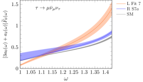
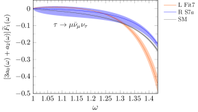
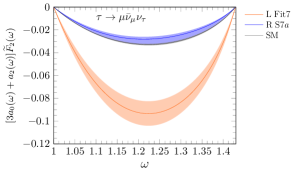
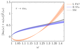
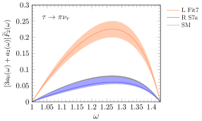
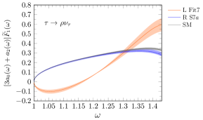
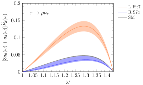
Figure 7: Results for the functions $n_{0}(\omega)\widetilde{F}^{d}_{0,1,2}(\omega)$ evaluated for the $\bar{B}\to D\tau(\mu\bar{\nu}_{\mu}\nu_{\tau},\pi\nu_{\tau},\rho\nu_{\tau})\bar{\nu}_{\tau}$ decays, keeping $y=m_{\mu,\pi,\rho}/m_{\tau}$ finite, and obtained within the SM and the beyond the SM scenarios of Fits 7 and 7a of Refs. Murgui et al. (2019) and Mandal et al. (2020), which only includes left- (right-)handed neutrino NP operators, respectively. Error bands account for uncertainties induced by both form-factors and fitted Wilson coefficients (added in quadrature).

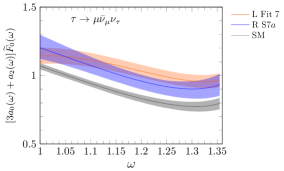
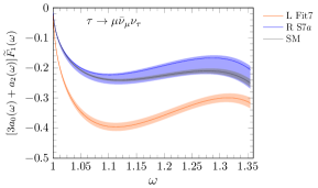
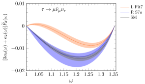
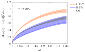
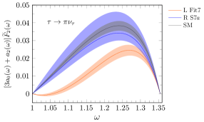
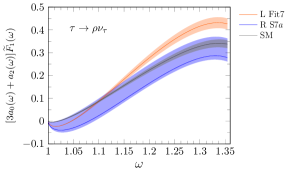
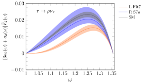
Figure 8: Same as in Fig. 7, but for the $\bar{B}\to D^{*}\tau(\mu\bar{\nu}_{\mu}\nu_{\tau},\pi\nu_{\tau},\rho\nu_{\tau})\bar{\nu}_{\tau}$ decays.

In this appendix we collect some results for the $\bar{B}\to D^{(*)}\tau(\mu\bar{\nu}_{\mu}\nu_{\tau}\pi\nu_{\tau},\rho\nu_{\tau})\bar{\nu}_{\tau}$ sequential decays. We start by showing, in Figs. 7 and 8, the $\widetilde{F}^{d}_{0,1,2}(\omega)$ functions evaluated within the SM and the NP models corresponding to Fit 7 of Ref Murgui et al. (2019) and Fit 7a of Ref Mandal et al. (2020), which only includes left- (right-)handed neutrino NP operators, respectively. Similarly to the $\Lambda_{b}\to\Lambda_{c}$ decay, the results for Fit 7 are very different from those obtained with Fit 7a and the SM, the latter two agreeing within uncertainties.

In Figs. 9 and 10, we present now the $d\Gamma/d\cos\theta_{d}$ distributions predicted within the SM and the beyond the SM scenarios of Fits 7 and 7a of Refs. Murgui et al. (2019) and Mandal et al. (2020), respectively. The best discriminating power is reached for forward and backward emission in the $\tau$-hadron decay modes for the $\bar{B}\to D$ decay.

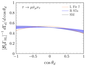
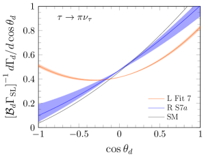
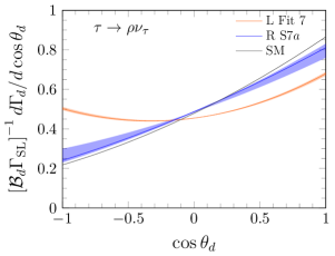
Figure 9: Angular $d\Gamma/d\cos\theta_{d}$ distribution for the $\bar{B}\to D\tau(\mu\bar{\nu}_{\mu}\nu_{\tau},\,\pi\nu_{\tau},\,\rho\nu_{\tau})\bar{\nu}_{\tau}$ decays, keeping $y=m_{d}/m_{\tau}$ to its finite value, and obtained within the SM and the beyond the SM scenarios of Fits 7 and 7a of Refs. Murgui et al. (2019) and Mandal et al. (2020), which only includes left- (right-)handed neutrino NP operators, respectively. Details as in Fig. 5.

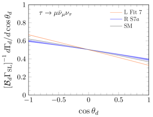
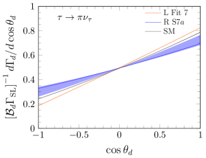
Figure 10: Same as in Fig. 9, but for the $\bar{B}\to D^{*}\tau(\mu\bar{\nu}_{\mu}\nu_{\tau},\pi\nu_{\tau},\rho\nu_{\tau})\bar{\nu}_{\tau}$ decays.

Finally, in Table 3, we collect the values for the integrated $\Gamma_{\tau}=\Gamma\left(\bar{B}\to D^{(*)}\tau\bar{\nu}_{\tau}\right)$ and $\Gamma_{e(\mu)}=\Gamma\left[\bar{B}\to D^{(*)}\,e(\mu)\bar{\nu}_{e(\mu)}\right]$ decay widths, as well as the ${\cal R}_{D^{(*)}}=\Gamma\left(\bar{B}\to D^{(*)}\tau\bar{\nu}_{\tau}\right)/\Gamma\left[\bar{B}\to D^{(*)}\,e(\mu)\bar{\nu}_{e(\mu)}\right]$ ratios, obtained in each of the physics scenarios considered in the figures. The corresponding results for the $\widehat{F}^{d}_{1,\,2}$ angular moments are given in Tables 4 and 5, for the lepton and hadron modes, respectively.

References

- Lees et al. (2012) J. P. Lees et al. (BaBar), Phys. Rev. Lett. 109, 101802 (2012), arXiv:1205.5442 [hep-ex] .
- Lees et al. (2013) J. P. Lees et al. (BaBar), Phys. Rev. D 88, 072012 (2013), arXiv:1303.0571 [hep-ex] .
- Huschle et al. (2015) M. Huschle et al. (Belle), Phys. Rev. D 92, 072014 (2015), arXiv:1507.03233 [hep-ex] .
- Sato et al. (2016) Y. Sato et al. (Belle), Phys. Rev. D 94, 072007 (2016), arXiv:1607.07923 [hep-ex] .
- Hirose et al. (2017) S. Hirose et al. (Belle), Phys. Rev. Lett. 118, 211801 (2017), arXiv:1612.00529 [hep-ex] .
- Caria et al. (2020) G. Caria et al. (Belle), Phys. Rev. Lett. 124, 161803 (2020), arXiv:1910.05864 [hep-ex] .
- Aaij et al. (2015) R. Aaij et al. (LHCb), Phys. Rev. Lett. 115, 111803 (2015), [Erratum: Phys.Rev.Lett. 115, 159901 (2015)], arXiv:1506.08614 [hep-ex] .
- Aaij et al. (2018a) R. Aaij et al. (LHCb), Phys. Rev. Lett. 120, 171802 (2018a), arXiv:1708.08856 [hep-ex] .
- Aaij et al. (2018b) R. Aaij et al. (LHCb), Phys. Rev. D 97, 072013 (2018b), arXiv:1711.02505 [hep-ex] .
- Amhis et al. (2021) Y. S. Amhis et al. (HFLAV), Eur. Phys. J. C 81, 226 (2021), arXiv:1909.12524 [hep-ex] .
- Aaij et al. (2018c) R. Aaij et al. (LHCb), Phys. Rev. Lett. 120, 121801 (2018c), arXiv:1711.05623 [hep-ex] .
- Anisimov et al. (1999) A. Y. Anisimov, I. M. Narodetsky, C. Semay, and B. Silvestre-Brac, Phys. Lett. B452, 129 (1999), arXiv:hep-ph/9812514 [hep-ph] .
- Ivanov et al. (2006) M. A. Ivanov, J. G. Korner, and P. Santorelli, Phys. Rev. D73, 054024 (2006), arXiv:hep-ph/0602050 [hep-ph] .
- Hernández et al. (2006) E. Hernández, J. Nieves, and J. Verde-Velasco, Phys. Rev. D 74, 074008 (2006), arXiv:hep-ph/0607150 .
- Huang and Zuo (2007) T. Huang and F. Zuo, Eur. Phys. J. C51, 833 (2007), arXiv:hep-ph/0702147 [HEP-PH] .
- Wang et al. (2009) W. Wang, Y.-L. Shen, and C.-D. Lu, Phys. Rev. D79, 054012 (2009), arXiv:0811.3748 [hep-ph] .
- Wang et al. (2013) W.-F. Wang, Y.-Y. Fan, and Z.-J. Xiao, Chin. Phys. C37, 093102 (2013), arXiv:1212.5903 [hep-ph] .
- Watanabe (2018) R. Watanabe, Phys. Lett. B 776, 5 (2018), arXiv:1709.08644 [hep-ph] .
- Issadykov and Ivanov (2018) A. Issadykov and M. A. Ivanov, Phys. Lett. B783, 178 (2018), arXiv:1804.00472 [hep-ph] .
- Tran et al. (2018) C.-T. Tran, M. A. Ivanov, J. G. Körner, and P. Santorelli, Phys. Rev. D97, 054014 (2018), arXiv:1801.06927 [hep-ph] .
- Hu et al. (2020) X.-Q. Hu, S.-P. Jin, and Z.-J. Xiao, Chin. Phys. C44, 023104 (2020), arXiv:1904.07530 [hep-ph] .
- Leljak et al. (2019) D. Leljak, B. Melic, and M. Patra, JHEP 05, 094 (2019), arXiv:1901.08368 [hep-ph] .
- Azizi et al. (2019) K. Azizi, Y. Sarac, and H. Sundu, Phys. Rev. D99, 113004 (2019), arXiv:1904.08267 [hep-ph] .
- Wang and Zhu (2019) W. Wang and R. Zhu, Int. J. Mod. Phys. A 34, 1950195 (2019), arXiv:1808.10830 [hep-ph] .
- Abdesselam et al. (2019) A. Abdesselam et al. (Belle), in 10th International Workshop on the CKM Unitarity Triangle (2019) arXiv:1903.03102 [hep-ex] .
- Alonso et al. (2017a) R. Alonso, B. Grinstein, and J. Martin Camalich, Phys. Rev. Lett. 118, 081802 (2017a), arXiv:1611.06676 [hep-ph] .
- Aaij et al. (2022) R. Aaij et al. (LHCb), (2022), arXiv:2201.03497 [hep-ex] .
- Detmold et al. (2015) W. Detmold, C. Lehner, and S. Meinel, Phys. Rev. D92, 034503 (2015), arXiv:1503.01421 [hep-lat] .
- (29) Marco Pappagallo (LHCB deputy physics coordinator) private communication .
- Nierste et al. (2008) U. Nierste, S. Trine, and S. Westhoff, Phys. Rev. D 78, 015006 (2008), arXiv:0801.4938 [hep-ph] .
- Tanaka and Watanabe (2013) M. Tanaka and R. Watanabe, Phys. Rev. D 87, 034028 (2013), arXiv:1212.1878 [hep-ph] .
- Fajfer et al. (2012) S. Fajfer, J. F. Kamenik, and I. Nisandzic, Phys. Rev. D85, 094025 (2012), arXiv:1203.2654 [hep-ph] .
- Duraisamy and Datta (2013) M. Duraisamy and A. Datta, JHEP 09, 059 (2013), arXiv:1302.7031 [hep-ph] .
- Duraisamy et al. (2014) M. Duraisamy, P. Sharma, and A. Datta, Phys. Rev. D 90, 074013 (2014), arXiv:1405.3719 [hep-ph] .
- Becirevic et al. (2019) D. Becirevic, S. Fajfer, I. Nisandzic, and A. Tayduganov, Nucl. Phys. B 946, 114707 (2019), arXiv:1602.03030 [hep-ph] .
- Ligeti et al. (2017) Z. Ligeti, M. Papucci, and D. J. Robinson, JHEP 01, 083 (2017), arXiv:1610.02045 [hep-ph] .
- Ivanov et al. (2017) M. A. Ivanov, J. G. Körner, and C.-T. Tran, Phys. Rev. D 95, 036021 (2017), arXiv:1701.02937 [hep-ph] .
- Bernlochner et al. (2017) F. U. Bernlochner, Z. Ligeti, M. Papucci, and D. J. Robinson, Phys. Rev. D95, 115008 (2017), [erratum: Phys. Rev.D97,no.5,059902(2018)], arXiv:1703.05330 [hep-ph] .
- Blanke et al. (2019a) M. Blanke, A. Crivellin, S. de Boer, T. Kitahara, M. Moscati, U. Nierste, and I. Nišandžić, Phys. Rev. D99, 075006 (2019a), arXiv:1811.09603 [hep-ph] .
- Bhattacharya et al. (2019) S. Bhattacharya, S. Nandi, and S. Kumar Patra, Eur. Phys. J. C 79, 268 (2019), arXiv:1805.08222 [hep-ph] .
- Colangelo and De Fazio (2018) P. Colangelo and F. De Fazio, JHEP 06, 082 (2018), arXiv:1801.10468 [hep-ph] .
- Murgui et al. (2019) C. Murgui, A. Penũelas, M. Jung, and A. Pich, JHEP 09, 103 (2019), arXiv:1904.09311 [hep-ph] .
- Shi et al. (2019) R.-X. Shi, L.-S. Geng, B. Grinstein, S. Jäger, and J. Martin Camalich, JHEP 12, 065 (2019), arXiv:1905.08498 [hep-ph] .
- Alok et al. (2020) A. K. Alok, D. Kumar, S. Kumbhakar, and S. Uma Sankar, Nucl. Phys. B 953, 114957 (2020), arXiv:1903.10486 [hep-ph] .
- Mandal et al. (2020) R. Mandal, C. Murgui, A. Peñuelas, and A. Pich, JHEP 08, 022 (2020), arXiv:2004.06726 [hep-ph] .
- Kumbhakar (2021) S. Kumbhakar, Nucl. Phys. B 963, 115297 (2021), arXiv:2007.08132 [hep-ph] .
- Iguro and Watanabe (2020) S. Iguro and R. Watanabe, JHEP 08, 006 (2020), arXiv:2004.10208 [hep-ph] .
- Bhattacharya et al. (2020) B. Bhattacharya, A. Datta, S. Kamali, and D. London, JHEP 07, 194 (2020), arXiv:2005.03032 [hep-ph] .
- Penalva et al. (2021a) N. Penalva, E. Hernández, and J. Nieves, JHEP 06, 118 (2021a), arXiv:2103.01857 [hep-ph] .
- Penalva et al. (2020a) N. Penalva, E. Hernández, and J. Nieves, Phys. Rev. D 102, 096016 (2020a), arXiv:2007.12590 [hep-ph] .
- Dutta and Bhol (2017) R. Dutta and A. Bhol, Phys. Rev. D 96, 076001 (2017), arXiv:1701.08598 [hep-ph] .
- Harrison et al. (2020) J. Harrison, C. T. Davies, and A. Lytle (LATTICE-HPQCD), Phys. Rev. Lett. 125, 222003 (2020), arXiv:2007.06956 [hep-lat] .
- Dutta (2016) R. Dutta, Phys. Rev. D 93, 054003 (2016), arXiv:1512.04034 [hep-ph] .
- Shivashankara et al. (2015) S. Shivashankara, W. Wu, and A. Datta, Phys. Rev. D 91, 115003 (2015), arXiv:1502.07230 [hep-ph] .
- Li et al. (2017) X.-Q. Li, Y.-D. Yang, and X. Zhang, JHEP 02, 068 (2017), arXiv:1611.01635 [hep-ph] .
- Datta et al. (2017) A. Datta, S. Kamali, S. Meinel, and A. Rashed, JHEP 08, 131 (2017), arXiv:1702.02243 [hep-ph] .
- Ray et al. (2019) A. Ray, S. Sahoo, and R. Mohanta, Phys. Rev. D99, 015015 (2019), arXiv:1812.08314 [hep-ph] .
- Bernlochner et al. (2019) F. U. Bernlochner, Z. Ligeti, D. J. Robinson, and W. L. Sutcliffe, Phys. Rev. D99, 055008 (2019), arXiv:1812.07593 [hep-ph] .
- Di Salvo et al. (2018) E. Di Salvo, F. Fontanelli, and Z. J. Ajaltouni, Int. J. Mod. Phys. A33, 1850169 (2018), arXiv:1804.05592 [hep-ph] .
- Blanke et al. (2019b) M. Blanke, A. Crivellin, T. Kitahara, M. Moscati, U. Nierste, and I. Nišandžić, Phys. Rev. D100, 035035 (2019b), arXiv:1905.08253 [hep-ph] .
- Böer et al. (2019) P. Böer, A. Kokulu, J.-N. Toelstede, and D. van Dyk, (2019), arXiv:1907.12554 [hep-ph] .
- Mu et al. (2019) X.-L. Mu, Y. Li, Z.-T. Zou, and B. Zhu, Phys. Rev. D 100, 113004 (2019), arXiv:1909.10769 [hep-ph] .
- Hu et al. (2021) Q.-Y. Hu, X.-Q. Li, Y.-D. Yang, and D.-H. Zheng, JHEP 02, 183 (2021), arXiv:2011.05912 [hep-ph] .
- Penalva et al. (2019) N. Penalva, E. Hernández, and J. Nieves, Phys. Rev. D100, 113007 (2019), arXiv:1908.02328 [hep-ph] .
- Penalva et al. (2020b) N. Penalva, E. Hernández, and J. Nieves, Phys. Rev. D 101, 113004 (2020b), arXiv:2004.08253 [hep-ph] .
- Alonso et al. (2016) R. Alonso, A. Kobach, and J. Martin Camalich, Phys. Rev. D 94, 094021 (2016), arXiv:1602.07671 [hep-ph] .
- Alonso et al. (2017b) R. Alonso, J. Martin Camalich, and S. Westhoff, Phys. Rev. D 95, 093006 (2017b), arXiv:1702.02773 [hep-ph] .
- Asadi et al. (2020) P. Asadi, A. Hallin, J. Martin Camalich, D. Shih, and S. Westhoff, Phys. Rev. D 102, 095028 (2020), arXiv:2006.16416 [hep-ph] .
- Penalva et al. (2021b) N. Penalva, E. Hernández, and J. Nieves, JHEP 10, 122 (2021b), arXiv:2107.13406 [hep-ph] .
- Tanaka and Watanabe (2010) M. Tanaka and R. Watanabe, Phys. Rev. D 82, 034027 (2010), arXiv:1005.4306 [hep-ph] .
- Cerri et al. (2019) A. Cerri et al., “Report from Working Group 4: Opportunities in Flavour Physics at the HL-LHC and HE-LHC,” in Report on the Physics at the HL-LHC,and Perspectives for the HE-LHC, Vol. 7, edited by A. Dainese, M. Mangano, A. B. Meyer, A. Nisati, G. Salam, and M. A. Vesterinen (2019) pp. 867–1158, arXiv:1812.07638 [hep-ph] .