ACE SWICS observations of solar cycle variations of the solar wind

Abstract

In the present work we utilize ACE/SWICS in-situ measurements of the properties of the solar wind outside ICMEs in order to determine whether, and to what extent are the solar wind properties affected by the solar cycle. We focus on proton temperatures and densities, ion temperatures and differential speeds, charge state distributions and both relative and absolute elemental abundances. We carry out this work dividing the wind in velocity bins to investigate how winds at different speeds react to the solar cycle. We also repeat this study, when possible, to the subset of SWICS measurements less affected by Coulomb collisions. We find that with the only exception of differential speeds (for which we do not have enough measurements) all wind properties change as a function of the solar cycle. Our results point towards a scenario where both the slow and fast solar wind are accelerated by waves, but originate from different sources (open/closed magnetic structures for the fast/slow wind, respectively) whose relative contribution changes along the solar cycle. We also find that the signatures of heating and acceleration on one side, and of the FIP effect on the other, indicate that wave-based plasma heating, acceleration and fractionation remain active throughout the solar cycle, but decrease their effectiveness in all winds, although the slow wind is much affected than the fast one.

1 Introduction

The solar wind consists of a continuous stream of supersonic particles flowing from the Sun into the Heliosphere, which shapes the physical properties of the interplanetary space and plays a fundamental role in Space Weather. In fact, the solar wind sets the stage for the propagation of Interplanetary Coronal Mass Ejections (ICMEs), influences some of their properties and their arrival time at the Earth, and in part it determines the overall effects that ICMEs have on the Earth’s magnetic field as Space Weather events. Also, the solar wind is capable of generating Space Weather events of its own, when faster wind streams overtake slower ones and create streams of shocked materials which can also affect the Earth’s magnetic field. Space Weather events represent a serious threat to our technological society, which is only destined to grow as modern civilization becomes more and more reliant on energy distribution, communication systems and space assets that can be directly damaged or even disabled by the effects of a Space Weather event such as ground induced currents, energetic particles, and ionospheric disturbances. The importance of the solar wind makes it imperative to develop a Space Weather forecast system capable of giving advance warning of an incoming solar storm and a robust understanding of the solar wind phenomenon itself.

The solar wind is a phenomenon most likely tied to the magnetic field in the atmosphere of the Sun. In fact, different magnetic field configurations are thought to give rise to different types of wind (e.g. Cranmer 2009 and references therein). Still, the solar magnetic field undergoes an 11-year cycle that radically changes its morphology and in turn the properties of the solar wind it sustains. The most spectacular indication of such a time dependent variation comes from the measurements carried out by the Ulysses spacecraft during its three polar passes in 1996 (solar minimum), 2001 (solar maximum) and 2008 (solar minimum) clearly showing how the spatial distribution of fast ($v>700$ km s^-1) and slow ($v<500$ /ms) wind completely changes during solar maximum and minimum (McComas et al. 1998, 2008). As in-situ measurements of the solar wind date back for decades, multiple studies have helped determine its properties evolve during the solar cycle.

2 Solar cycle dependence of solar wind properties

2.1 Magnetic field

After a certain distance from the photosphere, the solar wind plasma $\beta$ is larger than 1, so that the wind plasma drags the solar magnetic field along as it travels in the heliosphere. This magnetic field is very important as it interacts with planetary magnetospheres during both quiescence and storms. Since the magnetic field of the Sun changes along the solar cycle, the question is whether also the magnetic field of the solar wind shows a solar cycle variability. Zerbo & Richardson (2015) studied 27-day running averages of the solar wind magnetic field strength as measured near Earth and compared them with the variations of the sunspot number (as a proxy of the solar cycle) for the last five solar cycles (20 to 24). They found that the wind average magnetic field strength does correlate with the phase of the solar cycle, being larger during maximum and smaller during minimum. Furthermore, they found that the distribution of daily averages measured during a 1-year interval was the same at each of the solar minima with the only exception of the minimum of cycle 24, when the shape of the distribution was still the same but peaked at a lower value (3 G instead of 5 G). On the contrary, the distributions during solar maxima were very similar.

Owens et al. (2016a) utilized indirect proxies of the solar wind magnetic field to extend the period over which its time variation could be studied, reaching as far back as 1750. They provided estimates of the annual average wind magnetic field and successfully compared their results with direct estimates from the OMNI spacecraft observations. They confirmed the correlation between wind field magnitude and sunspot number found by Zerbo & Richardson and showed that a similar correlation existed as far down as 1750. Furthermore, they also showed that longer term variations exist, where the wind magnetic field minimum and maximum values change over multiple cycles, showing that the very low value of cycle 24 is actually similar to the values obtained around 1900, and that the large maximum values from 1950 to 1990 (with the exception of 1970) are similar to those occurred in 1860. Unfortunately, the 250-year time span they covered is still too short to determine whether multiple periodicities were present. In all cases, the wind magnetic field values varied in the 4-10 G range, showing that the solar cycle can alter the average wind field by a factor at least 2.

2.2 Dynamical properties

Zerbo & Richardson (2015) also tried to correlate the 27-day averages of the wind speed, density and mass flux with the sunspot number, finding that the correlation was much weaker than for the magnetic field and on the overall not much significant. Using the same dataset, Yermolaev et al. (2021) found an overall decrease of the main plasma parameters in the solar wind from cycle 22 to 23, which have then remained low during cycles 23 and 24. Still, a marked solar cycle distribution of the source regions of the wind near the ecliptic was noted by Luhmann et al. (2002), who found that polar coronal holes contributed to the wind in the ecliptic for only half of the solar cycle around solar minima, while during maxima the wind came from equatorial sources.

However, the OMNI measurements they used only allowed for measurements near the Earth. Using a completely different method, Lamy et al. (2017) were able to paint a much more complete picture for the mass flux. They used Ly-$\alpha$ backscattering measured by the SOHO/SWAN instrument (Bertaux et al. 1995) from 1996 to 2014 to determine the mass flux of the solar wind. Lamy et al. (2017) obtained maps of the distribution of the solar mass flux with longitude for every Carrington Rotation from 1996 to 2014. They found that the mass flux had a clear heliolatitudinal distribution, which changed as a function of the solar cycle phase: during minimum, the largest portion of the mass flux was concentrated within 20 degrees from the equator, with the fast wind filling the rest of the heliosphere with a much smaller mass flux; during maximum the slower, denser solar wind increased the absolute value of the mass flux, and was distributed over all latitudes.

The solar cycle dependence of both the latitudinal coverage and the absolute value of the mass flux cause the total solar mass loss to the solar wind to strongly depend on the solar cycle. An independent estimate of the total solar mass loss rate by Wang (1998) indicated that it varied from 2$\times 10^{-14}~{}M_{sun}/yr$ at the minimum to 3$\times 10^{-14}~{}M_{sun}/yr$ at the maximum during solar cycles 21 and 22. The variations in magnitude and spatial distribution of mass loss to the solar wind is very important, as the presence of denser solar wind material at all latitudes during solar maximum causes the rate of cosmic rates reaching the Earth to decrease, while during minimum the decreased protection of solar wind material causes the rate of galactic cosmic ray arrival at Earth to increase. For example, Fludra (2015) showed that the number of galactic cosmic ray hits affecting the detectors of the SoHO/CDS instrument orbiting at L1 was clearly dependent on the solar cycle, with the very weak minimum of cycle 24 recording a larger number of cosmic ray hits than the previous, stronger minimum.

Last, solar cycle variations in wind density and distribution also affect the torque exerted by the solar wind on the Sun. Finley et al. (2018) utilized three different methods to calculate the angular momentum loss of the Sun, yielding results that, while providing different average values, all clearly indicated a marked solar cycle variation, with the value of the torque increasing by a factor 3-5 from minimum to maximum.

2.3 Elemental composition

Elemental abundances are a very important solar wind parameter for two main reasons. First, once the solar wind accelerates away from the Sun, they are supposed to remain unaltered as the plasma travels into the Heliosphere, so that the values measured in-situ can be used to identify the plasma parcel’s source region. Second, elemental abundances in the lower solar atmosphere are different from their photospheric counterparts: differences depend on each element’s first ionization potential (FIP) being larger (high-FIP) or smaller (low-FIP) than 10 eV. In fact, the low-FIP/high-FIP ratio measured in the solar corona is enhanced by a factor (called FIP bias) dependent on the region’s magnetic field configuration. Usually, in open field configurations such as coronal holes the FIP bias is around unity (that is, no enhancement) while in closed field configurations it is anywhere between 2 and 5, possibly depending on time. These abundance changes, called FIP effect (Laming 2015), are thought to be due to ponderomotive forces tied to the same type of magnetic waves that are also one of the candidate entities responsible for solar wind heating and acceleration. Thus, studying the elemental abundances of the solar wind can provide precious information also on magnetic waves at the base of the solar corona, where the elemental fractionation takes place.

There are two ways of measuring solar composition: the abundance of an element relative to Hydrogen, also known as absolute abundances (e.g. C/H), and the abundance of an element relative to another element other than Hydrogen, named relative abundances, e.g. Ne/O. The former are tied to the metallicity of the Sun, the latter are affected by the FIP effect.

Since the FIP effect seems to be related to the magnetic field, it is fair to expect that it might be affected by the solar magnetic cycle. Several authors investigated the variation of abundance ratios of several key elements. For example, Kasper et al. (2007, 2012) utilized WIND measurements of the $\alpha$/proton ratio as a function of time from 1995 to 2010, thus capturing two solar minima and the maximum of solar cycle 23, finding a very strong dependence. Most importantly, they found that the time variation of this ratio was strongly dependent on the wind speed: the slower the speed, the larger the solar cycle sensitivity. With the only exception of the wind faster than 560 km s^-1, which showed a remarkable stability throughout the solar cycle, the $\alpha$/proton ratio decreased during minimum and reached a maximum of around 0.05 during maximum: the slowest speed wind ($v<300$ km s^-1) decreased this ratio by a factor 5-10 and the ratio was lower during the minimum of solar cycle 24 in 2008 than it was in the minimum of cycle 23 in 1996. To make the 2008 minimum even more peculiar, even the fastest wind showed a decrease in the $\alpha$/proton ratio during 2008-2009 that it did not show during the previous minimum of 1996-1997. The analysis of Kasper et al. (2008,2012) stops at 2010, but results were extended until 2015 and confirmed for the rising phase of cycle 24 by Zerbo & Richardson (2015).

Lepri et al. (2013) carried out a similar study utilizing data from the ACE/SWICS instrument in the 1998-2011 range, to determine the solar cycle variation of the abundances of heavy elements detected in-situ at 1 AU. They only divided the solar wind in two velocity classes (faster and slower than 500 km s^-1) and found that there is a $\approx$50% decrease in the abundances of He, C, O, Si, and Fe relative to H as the Sun moved towards the minimum of cycle 24, indicating a decrease of the wind’s metallicity; also, the FIP bias in the fast solar wind showed some variations indicating changes in the efficacy of the FIP effect in the fast wind’s source regions. Other signs of solar-cycle induced changes in the wind composition were found by Shearer et al. (2014) studying the Ne/O abundance ratio: this ratio is of critical importance for FIP fractionation models, for the Ne and O photospheric absolute abundances, and for helioseismological models of the solar interior. Shearer et al. (2014) found that the Ne/O ratio changed as a function of the solar cycle by factors also dependent on wind speed, being almost constant in the fast wind, and changing by a factor $\approx$1.5 in the slow wind: a similar variability was found by Landi & Testa (2015) in remote sensing observations of quiescent streamers, a possible source for the slow wind.

2.4 Charge state distributions

In-situ measurements of the charge state distribution of the solar wind have long been utilized to infer the conditions of the solar coronal region where the wind comes from. In fact, the solar wind undergoes electron-ion collisional ionization and recombination as it is accelerated from the source region in the heliosphere, traveling through a very steep initial temperature gradient in the solar transition region. As the plasma density decreases with distance, the efficiency of collisional processes decreases until a point is reached when the electron density is sufficiently low to effectively stop collisional ionization and recombination from occurring. From this point onward, the ionization status of the solar wind does not evolve and remains the same throughout the heliosphere. This point is called ”freeze-in” point, and its physical location depends on each element and each ion, as the ionization and recombination rates are different for species. Once frozen in, the charge state distribution of solar wind elements maintains a record of the electron density and temperature (which determine the local ionization and recombination rates) it has experienced before reaching the freeze-in point, as well of the wind speed, which determines how much time the wind spends in the densest regions where it can be ionized/recombined.

The most comprehensive study of the solar cycle dependence of the solar wind charge state distribution has been carried out by Lepri et al. (2013), who studied the charge state ratios of C, O and the average charge state of Fe. They found that both the fast and slow solar wind change their ionic composition as a function of the solar cycle, decreasing it during solar minimum; changes were largest for the less dense fast wind, but significant for both. Differences were large enough to affect the use of charge state ratios such as $O^{7+}/O^{6+}$ to discriminate between fast and slow solar wind, as slow wind ratio values at solar minimum were the same as fast wind values during solar maximum. Landi & Lepri (2015) investigated the effect of solar-cycle variations of photoionizing X-ray, EUV and UV flux on the solar wind ionization status, finding that it accounted only for part of the variation, the rest being likely due to a change electron in density, temperature and wind speed.

2.5 Goal of the present work

The results obtained by Kasper et al. (2007, 2012) and Lepri et al. (2013) clearly demonstrate that the solar wind compositional plasma properties do depend on the solar cycle. However, the former focused on $\alpha$ particles only, while Lepri et al. (2013) did not consider the two quantities that can provide information on the wind heating and acceleration processes: ion temperatures and differential velocities. Also, these studies did not investigate how collisional age (e.g. Tracy et al. 2015, 2016), an indication of the amount of Coulomb collisions experienced by a wind plasma parcel, affect the measured solar wind properties. Furthermore, Lepri et al. (2013) divided the solar wind in two broad velocity classes (separated at 500 km s^-1); however, as the dependence of ion temperatures and ionization status on wind speed is continuous rather than a step function, such broad velocity bins lose resolution in determining the speed dependence of these quantities.

Our goal is to improve on these earlier works by:

1. Dividing the wind in much finer velocity classes, to increase velocity resolution;

2. Including ion temperatures and differential wind speed in the analysis;

3. Investigating how the correlation of ion temperatures with charge-to-mass ratios, mass, and wind speed depends on the solar cycle;

4. Determining how lower collisional age influences the results.

The data and methodology we use are described in Section 3; results are reported in Section 4 and discussed in Section 5, while Section 6 summarizes this work.

3 Data and methodology

3.1 Instruments

The data used in the present work primarily come from the SWICS instrument (Gloeckler et al. 1998) on board the ACE satellite. We utilized the data collected from the start of the mission in 1998 to 2011, after which an anomaly in the hardware increased the background and generated several invalid measurements. The 1998-2011 time interval covers one full solar cycle, from the rising phase of cycle 23 to the rising phase of cycle 24. The data we used consist of bulk velocity, thermal speed, and density for the most abundant ions observed by SWICS: He²⁺, C^4-6+, N^5-7+, O^5-7+, Ne^6-9+ (with the exception of Ne⁷⁺, unavailable), and Fe^7-12+; we have used 2-hr averaged data. The thermal speed in this dataset only includes the component along the SWICS look direction.

Proton data have also been rebinned from the original 12-minute resolution to 2 hours by averaging them and re-normalizing in case some time stamps were missing; however, care was taken to ensure that the proton plasma properties were constant during each 2-hour time stamp. We first removed data where the error was larger than 0.4, then we removed all time stamps for which either the proton speed or proton temperature averages had a standard deviation larger than half of each quantity’s value.

Differential speeds between protons and heavy ions were measured only from plasma streams traveling within 10^o of the magnetic field direction. To select this sample, we utilized magnetic field measurements from the MAG instrument (Smith et al. 1998) on board ACE. Given the large variability of the magnetic field within two hours, we only kept the time stamps where the magnetic field was relatively constant; we selected these by calculating average magnetic field $B_{tot}$ and the standard deviation $\sigma_{B}$ and requiring that $sigma_{B}/B_{tot}<0.3$: this additional requirement greatly decreased the number of time stamps available for differential speed studies.

3.2 Data selection

To improve the quality of the sample, for each ion we utilized only time stamps with a number of counts larger than 15, except to determine the total abundance of an element, in which case we accepted time stamps where at least one ion of this element had more than 15 counts. Due to the fact that Oxygen is usually clustered in the O⁶⁺ charge state (which usually accounts for at least 80% of the element in all wind types) we did not use Oxygen in element abundance studies when O⁶⁺ did not have the required 15 counts.

Since we are interested in the background solar wind only, we have removed data taken during ICME events using the Richardson & Cane list (Cane & Richardson 2003, Richardson & Cane 2010); we further excluded wind streams not present in that list, which were either faster than 800 km/s, or with Fe¹⁶⁺/Fe ratio values larger than 0.1 or O⁷⁺/O⁶⁺ ratio values larger than 1.

In order to study the dependence of wind’s properties on the solar cycle with a high velocity resolution, we divided the 300-650 km s^-1velocity range in 14 velocity bins, each 25 km s^-1wide; we further created two more bins for the fast wind (650-700 km s^-1and 700-800 km s^-1) and one bin collecting all wind slower than 300 km s^-1. The width of these bins have been selected as a compromise between achieving high velocity resolution, while at the same time maintaining a significant number of events in each velocity bin. However, due to the lack of data in some velocity bins (e.g. 325-350 km s^-1in 2003 or 650-700 km s^-1in 2009), some gaps in the dataset are present.

3.3 Methodology

We study several properties of the solar wind as observed close to the ecliptic plane by ACE/SWICS in the entire 1998-2011 range. We aim at characterizing the behavior of an array of plasma properties with the goal of understanding whether and how the solar cycle affects the heating, acceleration, and evolution of the solar wind.

The element composition of the wind was studied both to determine the wind’s absolute and relative abundances. We study the latter to understand whether the abundance ratio of low-FIP to high-FIP elements (that is, the FIP bias) changes with time to investigate the FIP effect (Laming 2015). Also, we seek to understand whether the wind acceleration mechanisms are as effective at extracting heavy ions into the solar wind during the solar cycle as they are at accelerating protons.

Charge state composition provides information on the main quantities that determine the ionization status of the solar wind: plasma electron density, electron temperature and speed. The former two quantities determine the local efficency of free electrons at ionizing wind ions at any location before the freeze-in distance, while the latter determines the time that the wind spends being ionized at each location (Landi et al. 2012).

Ion temperatures and differential velocities are two signatures for wave-based wind heating and acceleration (Cranmer et al. 2008, Khabibrakhmanov & Mullan 1994, Cranmer et al. 1999, Chandran 2010, Kasper et al. 2013). In particular, ion kinetic temperature ratios to proton temperatures are expected to depend on ion parameters such as mass and charge/mass ratio due to the effect of waves, while heavy elements are predicted to stream faster than protons by up to an Alfven speed. Solar cycle dependence of these two parameters would indicate effects on the efficiency of waves at accelerating and heating the solar wind. However, these signatures tend to be erased by Coulomb collisions, which work toward equalizing ion and proton speeds, as well as ion and proton temperatures. For this reason, we have repeated, where the number of available data points made it possible, the study of these two quantities limiting the sample to plasma parcels whose collisional age $A_{C}$ (Tracy et al. 2015, 2016) is less than 0.3, where $A_{C}$ is defined as:

$$A_{C} = 2.19\times 10^{7}\frac{Z_{i}^{2}}{A_{i}}\frac{\ln\Lambda_{ip}}{i{\left({\frac{T_{i}}{A_{i}}+T_{p}}\right)}^{3/2}}\frac{n_{p}}{v_{p}}$$ (1)

$$\log\Lambda_{ip} = 29.9-\ln{{\left[{\frac{Z_{i}{\left({A_{i}+1}\right)}}{A_{i}T_{p}+T_{i}}{\sqrt{\frac{n_{i}Z_{i}^{2}}{T_{i}}+\frac{n_{p}}{T_{p}}}}}\right]}}$$ (2)

where $Z_{i}$ and $A_{i}$ and the ion’s charge and atomic number, $T_{i}$ and $T_{p}$ are the ion and proton temperatures (in K), $n_{i}$ and $n_{p}$ are the ion and proton densities (in cm^-3) and $v_{p}$ is the proton speed (in km s^-1). Large values of $A_{C}$ indicate that the wind plasma has undergone many Coulomb collisions before reaching the instrument, small values indicate a more pristine solar wind.

4 Results

4.1 Proton properties

Both proton temperature and density change as a function of time along the solar cycle. Also, the type and amount of change are different in different velocity classes.

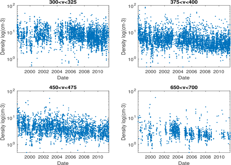
Figure 1: Proton density versus time for 4 velocity classes: slow wind (top row), intermediate wind (bottom left) and fast wind (bottom right).

Proton density shows a decrease over time which has two specific properties, as shown in Figure 1. First, the decrease is most evident at speeds larger than 350 km s^-1, while at lower speeds the proton density seems to be essentially constant. Second, the decrease is steady from 1998 to 2011, with no apparent correlation with the solar cycle phase, so that it seems to occur at time scales much larger than the cycle itself. Most remarkably, it does not show any hint of recovery after the minimum of cycle 24 in 2008.

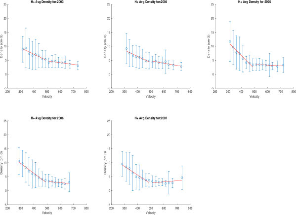
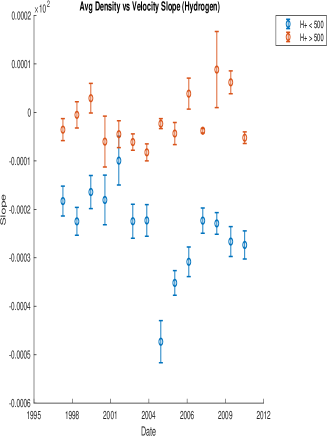
Figure 2: Left: Examples of double linear fit to the yearly averaged proton density vs. speed, for the years 2003 to 2007. Right: Slope of the linear fit to the yearly average proton density versus year. Red: velocity bins faster than 500 km s^-1. Blue: velocity bins slower than 500 km s^-1. See text for details.

Proton density has been long known to decrease as the wind speed increases: faster winds are more tenuous. We tested whether the solar cycle had any influence on the rate of such decrease: for each year, we averaged the proton density in each velocity bin and calculated a linear fit between average density and speed. We found that no satisfactory fit could be found that reproduced the whole range of speeds, as the density versus speed relationship seems to have a marked change in slope at around 500 km s^-1, as shown in Figure 2 (left): the proton density decreases faster below 500 km s^-1, while it seems to be almost constant at larger speeds. We then carried out two separate linear fits at speeds larger and smaller than 500 km s^-1, and show the slope of both fits as a function of time in the solar cycle in Figure 2 (right). Fitted slopes are different, with the wind faster than 500 km s^-1having an approximately constant density, but neither shows a significant dependence on the solar cycle, being approximately constant throughout the entire period under consideration.

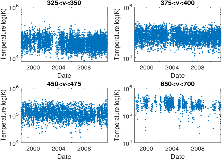
Figure 3: Proton temperature versus time for 4 velocity classes: slow wind (top row), intermediate wind (bottom left) and fast wind (bottom right).

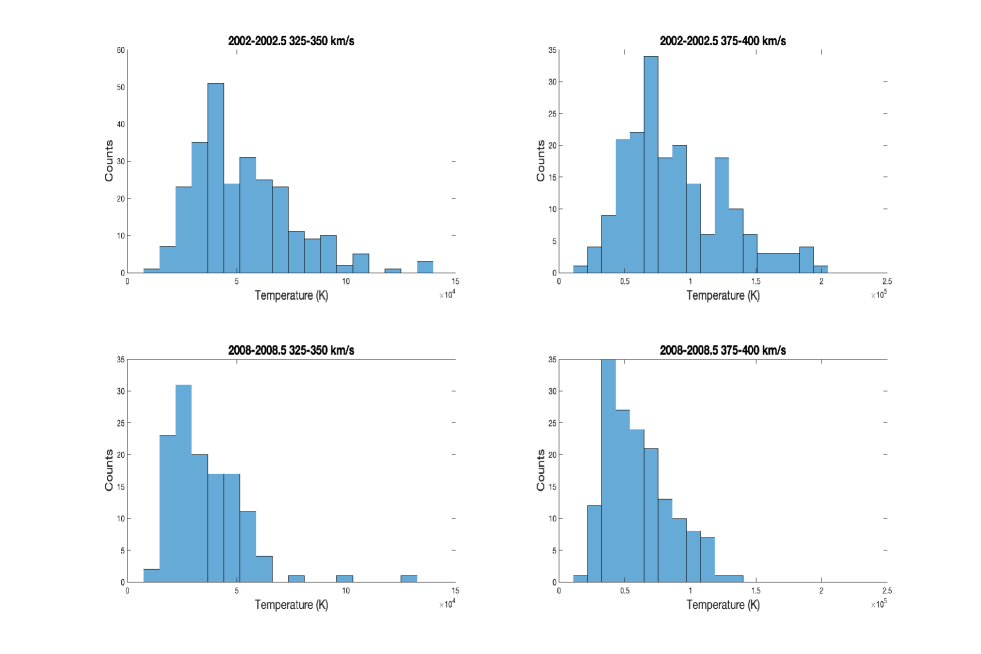
Figure 4: Histogram of proton temperatures for the 325-350 km s^-1(left column) and 375-400 km s^-1(right column) velocity classes, during solar maximum (year 2002-2002.5, top row) and solar minimum (year 2008-2008.5, bottom row).

Proton temperatures ($T_{p}$), on the contrary, are essentially constant with time at speeds larger than 400 km s^-1, with a value increasing with speed itself, as shown in Figure 3. On the contrary, at slower speeds $T_{p}$ shows some dependence on the cycle phase, being lower during the 2008-2009 minimum and larger during the 2000-2002 maximum. An example is shown in Figure 4, where at solar maximum $T_{p}$ peaks at larger temperatures (a bit less than a factor 2) and has a broader distribution than at solar minimum. At larger speeds the difference decreases until it disappears.

4.2 Elemental abundances

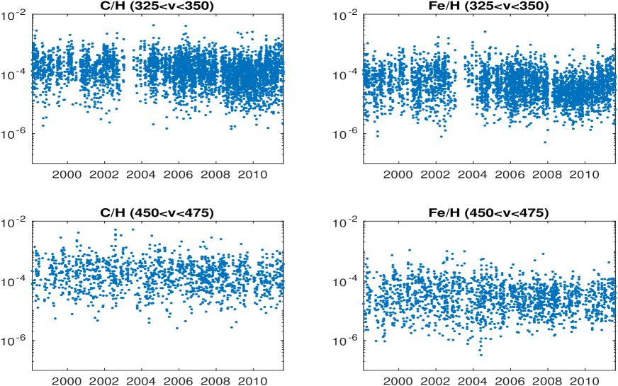
Figure 5: C/H (left panels) and Fe/H (right panels) abundance ratios as a function of time for two velocity classes: slow wind (325-350 km s^-1) and intermediate wind (450-475 km s^-1).

As far as absolute abundances are concerned, solar cycle variability occurs at speeds lower than 450 km s^-1, with the magnitude of change decreasing as the wind speed increases, as shown in Figure 5. In the slowest velocity bins, the abundances of C, N, O, Ne and Fe decrease around 2009, and seem to have recovered by 2010. At the lowest speeds, the decrease amounts to a factor 2-3.

The relative C/O abundance ratio is constant at $\approx$0.7 along the solar cycle, and has the same value in all velocity classes. Considering that the photospheric value of this ratio ranges between 0.45 and 0.55, this measurement indicates a FIP enhancement of C over O of $\approx$1.3-1.6; the stability of this value over the solar cycle indicates that the process enhancing C over to O is not affected by the solar cycle and is the same in all wind source regions.

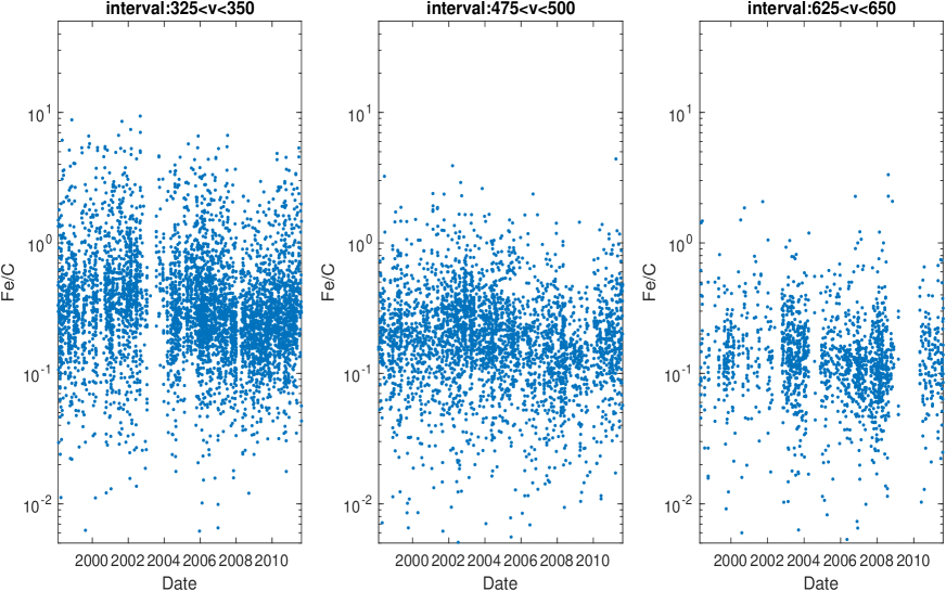
Figure 6: Relative Fe/C abundance as a function of time for slow (325-350 km s^-1, left), intermediate (475-500 km s^-1, middle) and fast (625-650 km s^-1, bottom) wind.

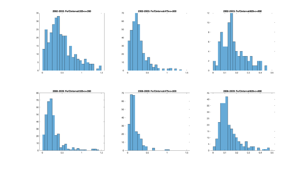
Figure 7: Histograms of the Fe/C abundance ratio during solar maximum (2003, top row) and minimum (2008, bottom row), for the 325-350 km s^-1(left column), 475-500 (middle column) and 625-650 km s^-1(right column) velocity bins.

The Fe/C relative abundance, on the contrary, changes as a function of time, as shown in Figure 6. Fe/C ratio values are lower during solar minimum, as noted by Lepri et al. (2013). Figure 7 shows Fe/C abundance ratio histograms for three different velocity bins during 2003 and 2008, providing a more quantitative estimate of the change; the effect is lower at larger speeds. It is also worth noting that the spread of values in these ratios is larger at lower speed, especially during solar maximum, and it decreases at larger speed. This is consistent with possible multiple sources of the slow solar wind, originating from plasmas with different composition (e.g. Stakhiv et al. 2015, 2016 and references therein).

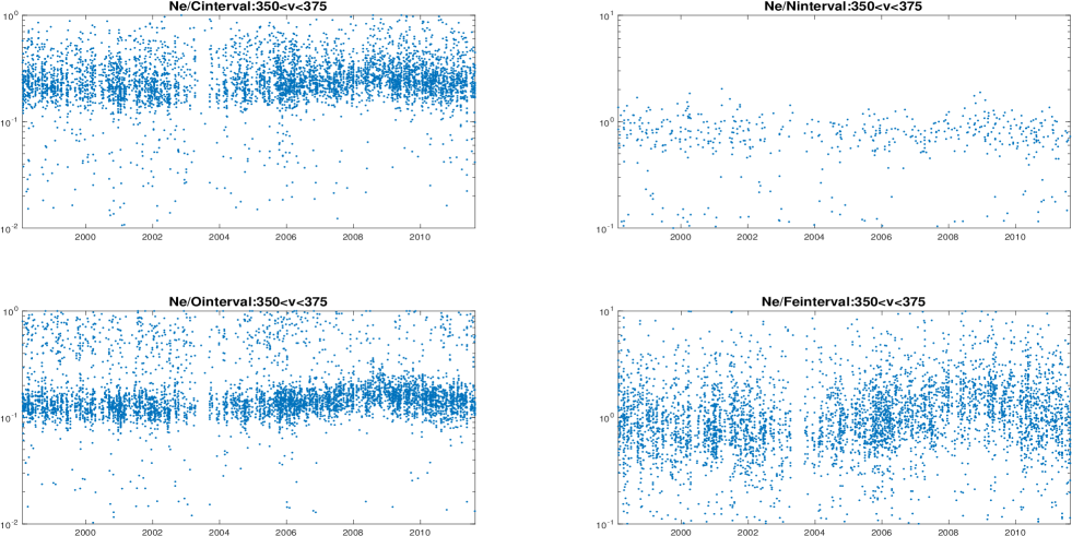
Figure 8: Ne abundance ratios as a function of the solar cycle for the 350-375 km s^-1velocity bin: Ne/C (top left), Ne/N (top right), Ne/O (bottom left) and Ne/Fe (bottom right).

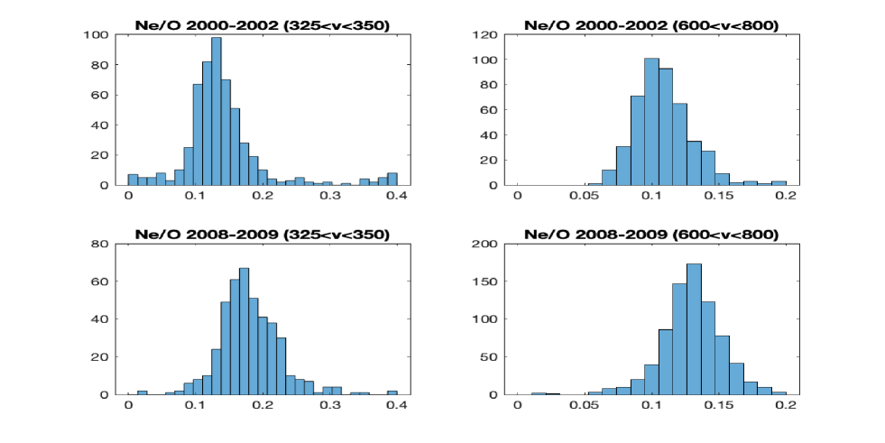
Figure 9: Histograms of the Ne/O abundance ratio during solar maximum (2000-2002, top row) and minimum (2008-2009, bottom row), for the 325-350 km s^-1(left column) and 650-700 km s^-1(right column) velocity bins.

Neon is a peculiar element because the Ne⁺⁷ charge state is hopelessly blended with the far more abundant O⁶⁺ charge state, to the point that it is not possible to determine its distribution from the raw measurements and thus measure its density. Shearer et al. (2014) discuss that the contribution of this charge state to the total Ne abundance is likely lower than 15% at solar minimum, where its abundance is expected to be largest, and less at solar maximum. Furthermore, Neon’s second most abundant isotope (²²Ne) accounts for $\approx$6.5% of the total Ne abundance, and this value seems to undergo fractionation between the fast and the slow solar wind (Heber et al. 2012). Thus, the elemental abundance of Ne is subject to additional uncertainties than other elements. With this in mind, the abundance ratios involving Ne have a peculiar behavior. The relative Ne/O abundance ratio is remarkably constant throughout the solar cycle, despite a small increase during the minimum of cycle 23 during 2008-2009, as shown in Figure 8; the increase is dependent on speed, being largest at a factor around 2 at the slowest speeds and decreasing at speeds of 500 km/s and larger (e.g. Figure 9). This trend was first described by Shearer et al. (2014), and resembled the Ne/O abundance ratio in quiescent streamers measured by Landi & Testa (2015). Interestingly, the Ne/C and Ne/N abundance ratios show a smaller increase at solar minimum than Ne/O. The Ne/Fe ratio instead combines both the apparent increase of Neon over the other high-FIP elements, and the decrease of Fe over those same elements, and thus shows a significant increase at low speeds during the 2007-2009 minimum. No discernible trends were found for the Ne/H ratio, as its value ranges over one order of magnitude at any speeds, and this variability masks any possible trend with the solar cycle.

4.3 Ion temperatures and temperature ratios

4.3.1 Absolute values

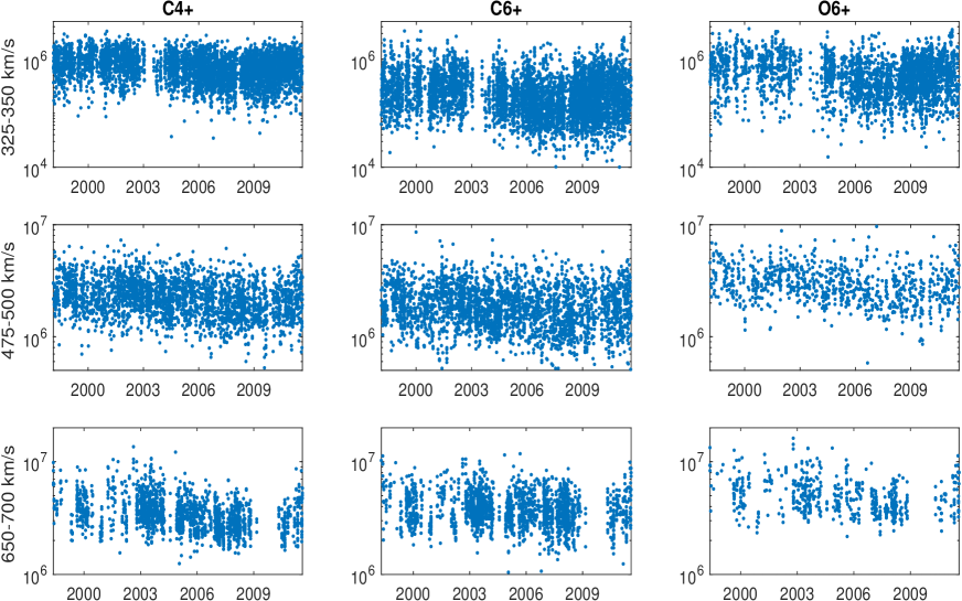
Figure 10: Ion temperature values for select C and O ions as a function of time for three velocity classes: slow (325-350 km s^-1), intermediate (450-475 km s^-1) and fast (650-700 km s^-1) wind.

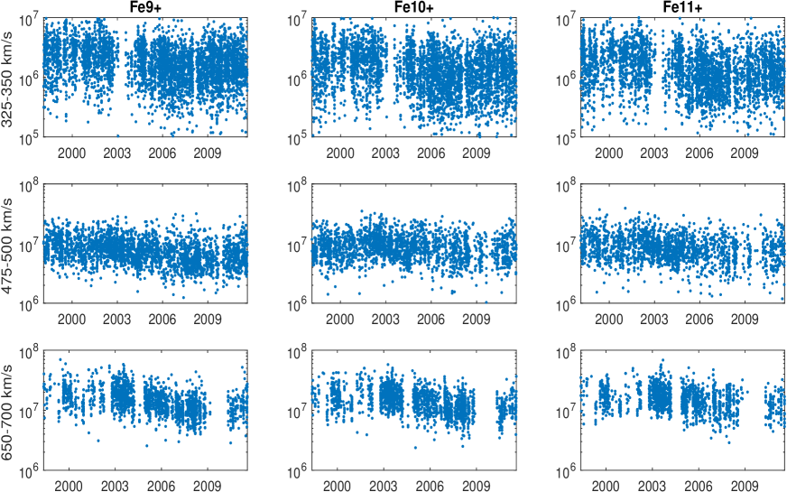
Figure 11: Ion temperature values for select Fe ions as a function of time for three velocity classes: slow (325-350 km s^-1), intermediate (450-475 km s^-1) and fast (650-700 km s^-1) wind.

The temperatures $T_{i}$ of all ions show at least some degree of variability with the solar cycle. Some examples are shown in Figures 10 and 11, which report values in three velocity classes (325-350, 475-500 and 650-700 km s^-1) for a few Carbon, Oxygen and Iron ions. Ion temperatures show a factor $\approx$1-3 decrease during solar minimum at all speeds, although the lack of solar wind in the faster speed bins between 2009 and 2010 prevents a definitive conclusion. Unfortunately, the lack of data before 1998 makes it impossible to determine whether such decrease occurs also during the previous minimum or was peculiar to the unusually weak cycle 24 minimum.

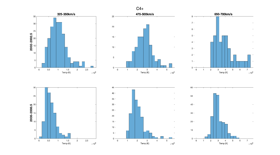
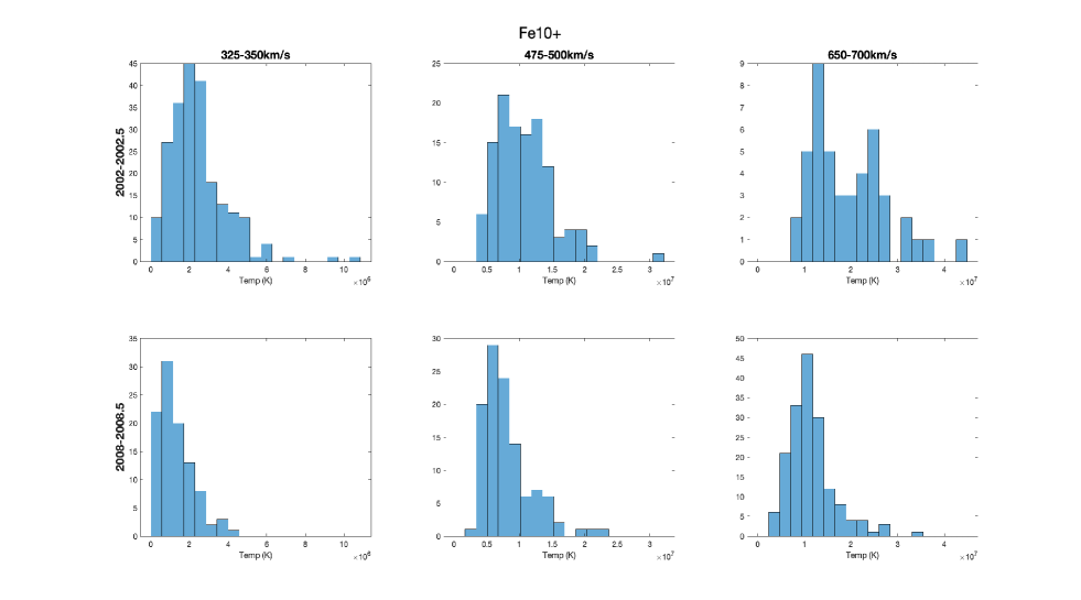
Figure 12: Histograms for the C⁴⁺ and Fe¹⁰⁺ ion temperature values in 2002-2005 (first and third rows) and 2008-2008.5 (second and bottom row) for three velocity classes: slow (325-350 km s^-1), intermediate (450-475 km s^-1) and fast (650-700 km s^-1) wind.

Figure 11 also shows that the spread in temperature values for each of the Fe ions displayed is much larger at lower speed, with values spanning approximately one order of magnitude while at larger speeds covering approximately a factor of three. Such a behavior is present to a lesser extent also in C and O, as shown in Figure 12 for C⁴⁺ and Fe¹⁰⁺.

4.3.2 Ion temperature vs speed

It has long been known that ion temperatures are larger in the fast wind, and decrease along with the wind speed – Figures 10 to 12 report some examples. The question is whether this empirical relationship changes along the solar cycle. To investigate this, for each ion we have averaged $T_{i}$ in yearly bins for every velocity class, and fitted the average T_ion vs speed relationship every year. We experimented with fitting two types of linear functions:

$$T_{ion} = a_{lin}\times v+b_{lin}$$ (3)

$$\log T_{ion} = a_{log}\times v+b_{log}$$ (4)

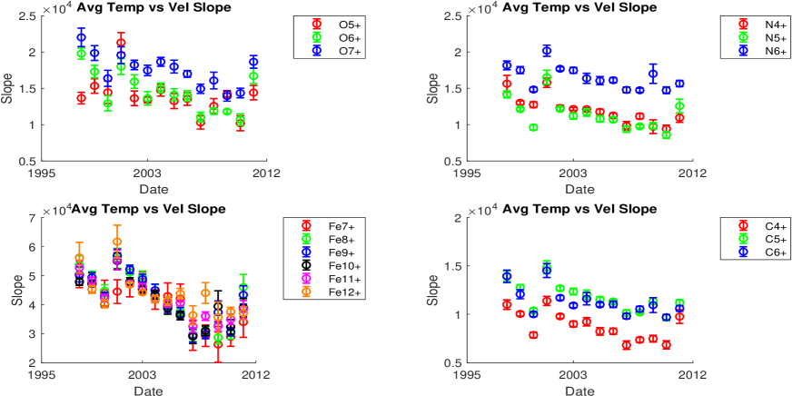
Figure 13: Value of $a_{lin}$ for C, N, O and Fe as a function time along the solar cycle.

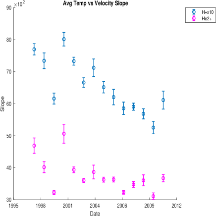
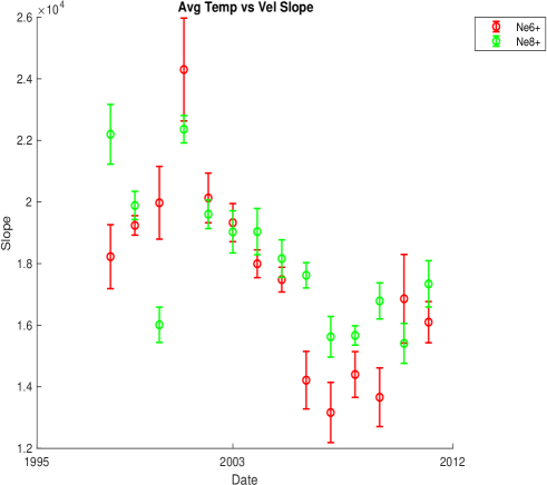
Figure 14: Value of $a_{lin}$ for protons (left) and select Neon ions (right) as a function time along the solar cycle.

We found that the correlation coefficient for Equation 3 was higher, so we analyzed the dependence of $a_{lin}$ along the solar cycle, which is shown in Figure 13 for C, N, O and Fe, and Figure 14 for H, He and Ne. Both figures indicate that there is a tendency of $a_{lin}$ to decrease from cycle 23 maximum to minimum in all these elements, the only exception being He²⁺ whose $a_{lin}$ value is essentially constant after 2002. Although the SWICS dataset we used only includes a small part of the beginning of solar cycle 24, there is some hint of a recovery of the pre-minimum slope values after 2009. This result is consistent with the ion temperature decreasing during solar minimum.

4.3.3 Ion temperature vs charge-to-mass ratio

Several heating mechanisms predict that ion temperatures depend on the charge-to-mass ratio (Landi & Cranmer 2009 and references therein). To test this dependence, and check whether such a dependence is affected by the solar cycle, we have fitted a relationship of the type

$$Log~{}T_{ion}=a_{Z/A}{\left({\frac{Z}{A}}\right)}+b_{Z/A}$$ (5)

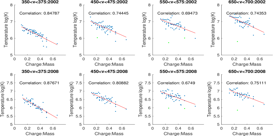
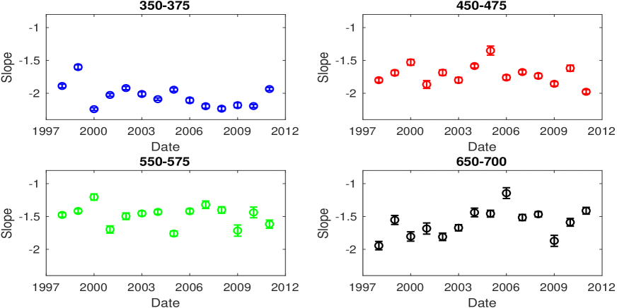
Figure 15: Top two panels: Annual averages of $\log T_{ion}$ vs the Z/A ratio, for four velocity classes in 2002 (first panel) and 2008 (second panel), along with a linear fit. Bottom two panels: value of the $a_{Z/A}$ slope as a function of time along the solar cycle, for each velocity class shown in the top two panels (see text for details).

to the annual averages of $T_{ion}$ in each velocity bin. Examples of the fit for four select velocity bins in 2002 (solar maximum) and 2008 (solar minimum) are shown in Figure 15 (top): the correlation coefficient is best at slower speeds, and decreases in the fast wind, although the fit is significant at all speeds. Figure 15 (bottom) displays the $a_{Z/A}$ coefficient as a function of the solar cycle for each of the four velocity bins in the top panel: there is no indication that $a_{Z/A}$ correlates either with velocity, or with the solar cycle.

Figure 15 (top) indicates that a few data points, marked in green, were discarded. These points were discarded when the difference between the average annual $T_{ion}$ value and the fitted one was larger than 0.5 dex: after being removed, the fit was re-done. These points correspond to three categories of ions:

1. Ions like C³⁺, Fe¹⁹⁺ and similar, with less than 5 counts to calculate the annual average $T_{ion}$: these ions were considered too uncertain;

2. He¹⁺: this ion has a relatively large number of annual counts to calculate an average, but Rivera et al. (2021) found that most of He¹⁺ may be formed in the inner Heliosphere by charge exchange interactions between wind $\alpha$ particles and outgassed Helium and Hydrogen originating from circumsolar dust, so its properties may be influenced by different processes than all the other ions and for this reason was removed from the fit;

3. He²⁺: the annual average $T_{ion}$ for this ion is consistenly lower than the fitted value by amounts of the order of 0.5 dex (so that sometimes it was not removed from the plot). We will further discuss this He²⁺ feature in Section 4.6.

4.3.4 Ion temperature vs mass

We also checked whether the ion-to-proton temperature ratio is mass-proportional, and whether such a dependence changes with the phase of the solar cycle. We found that no significant dependence was present. The ratio $T_{ion}/T_{p}/M_{ion}$ ranges between 1 and 2 for all the ions we considered with no specific trend. Within each element, different ionization stages had a different value in this range, consistently with the clear dependence of the $T_{ion}/T_{p}$ ratio on the Z/A ratio, but no trend was identified neither with ionization stage, nor with time along the solar cycle.

4.4 Differential velocity

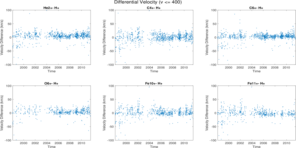
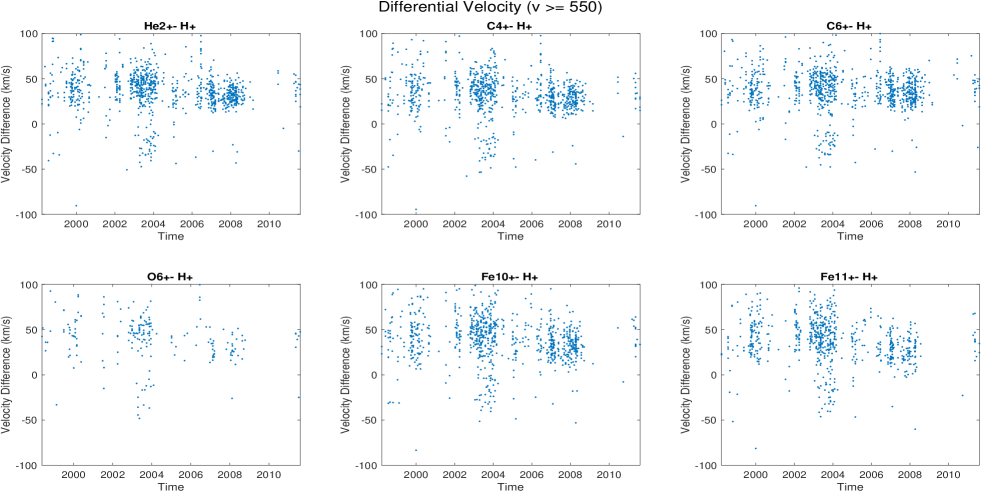
Figure 16: Differential velocities for a selection of ions along the solar cycle for velocities slower than 400 km s^-1(top two rows) and faster than 550 km s^-1(bottom two rows).

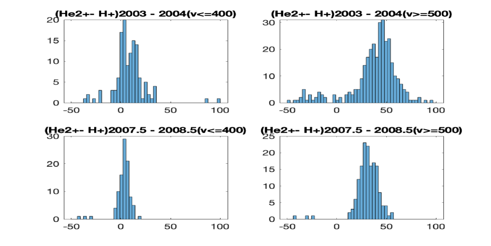
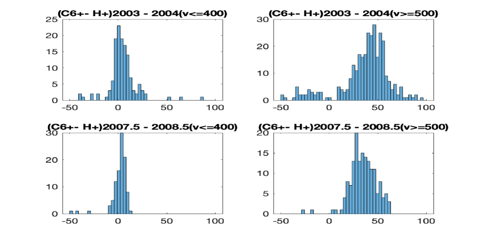
Figure 17: Differential velocities for a selection of ions along the solar cycle for velocities slower than 400 km s^-1(top two rows) and faster than 550 km s^-1(bottom two rows). Results are shown at solar maximum (first and third row) and minimum (second and fourth row).

Ion-proton differential velocity was measured using only plasma parcels where the radial component of the magnetic field was 90% or more of the total magnetic field magnitude, and that the magnetic field variability was limited within each 2-hour timebin. These requirements greatly decreased the number of data, so that resolution in velocity needed to be sacrificed in order to preserve a sufficient number of counts to let any trend be discernible. We divided the available data in two velocity classes, slow ($v<400$ km s^-1), and fast ($v>550$ km s^-1) in an effort to isolate fast and slow wind streams; even so, the number of available data points is very small. Results are shown in Figure 16, and example of histograms for He²⁺ and C⁶⁺ are shown in Figure 17.

Two main conclusions can be drawn from the data. At velocities slower than 400 km s^-1, differential velocity is smaller than 10-15 km s^-1 for all ions, and does not show any dependence on the solar cycle, remaining constant in this interval. At velocities larger than 550 km s^-1, speed differences range between 20 and 70 km s^-1, with only a moderate decrease during solar minimum. Furthermore, the lack of data did not allow us to determine whether there is any dependence of the differential speed on the ions’ charge, mass, or charge/mass ratio. The presence of a small population of measurements with negative speeds (e.g. ions are slower than protons) around 2004 for the fast wind class is a puzzle: we have investigated whether they could be due to magnetic switchbacks (Yamauchi et al. 2004) but an inspection of MAG data in the proximity of these points did not reveal a systematic presence of such magnetic structures.

4.5 Charge state composition

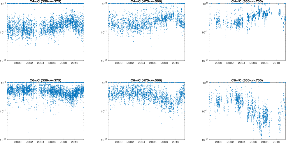
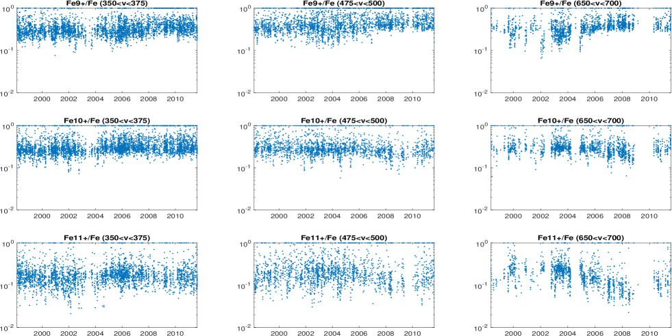
Figure 18: Relative abundances of a selection of C ions along the solar cycle, for three velocity classes ranging from slow, intermediate, and fast wind.

Figure 19: Relative abundances of a selection of Fe ions along the solar cycle, for three velocity classes ranging from slow, intermediate, and fast wind.

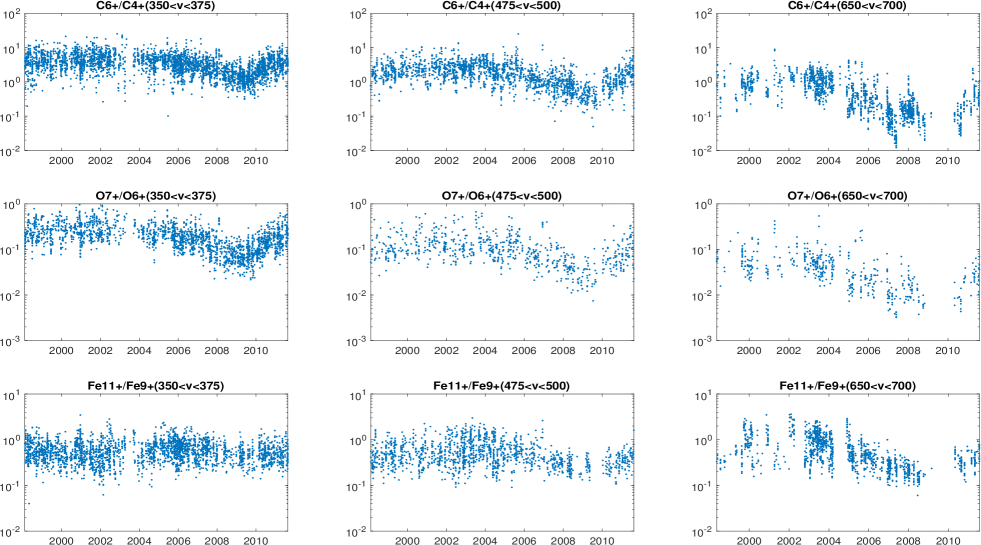
Figure 20: Select C and O charge state ratios along the solar cycle, for three velocity classes ranging from slow, intermediate, and fast wind.

Charge state composition strongly depends on the solar cycle, with all elements and ions showing higher ionization during maximum than during solar minimum with the only exception of Neon ions. A few examples are shown in Figures 19 and 19. As a consequence, charge state ratios show an even more marked dependence on the solar cycle, as shown in Figure 20. This behavior confirms the cycle-related variability of a few key charge state ratios noted by Lepri et al. (2013). It is important to note that such a behavior is also clearly shown by individual Fe ions and Fe charge state ratios, even though the average charge state of Fe does not strongly depend on the solar cycle: even though ionization changes from solar minimum to maximum are not as large as for Carbon and Oxygen ions, they are significant and indicate that the ionization status of Fe is also significantly changing with time. This last result shows that using the average charge states to characterize the ionization status of Fe dilutes the effects of the solar cycle on this element.

4.6 Low collisional age plasma

Proton-ion Coulomb collisions tend to equalize ion temperatures and differential velocity signatures in the solar wind, while they have no effect on charge state composition. Thus, restricting the analysis only to wind stream with collisional age $A_{C}<0.3$ allows us to investigate more pristine solar wind streams, whose properties are closer to those much closer to the Sun.

However, enforcing the $A_{C}<0.3$ limit to the data means that very few measurements were left in any velocity bin slower than 350 km s^-1, and that the number of surviving data is also reduced below 500 km s^-1. At larger speeds, all the trends we identified in the complete data set are confirmed, because removing the high collisional age streams did not affect the data set significantly since the plasma density is sufficiently low to always satisfy the $A_{C}<0.3$ criterion with the only exception of the densest streams.

At lower speed instead, the surviving data were too few to allow any investigation on differential velocity. On the contrary, sufficient data were left to repeat our study of the ion temperatures.

4.6.1 Ion temperature values

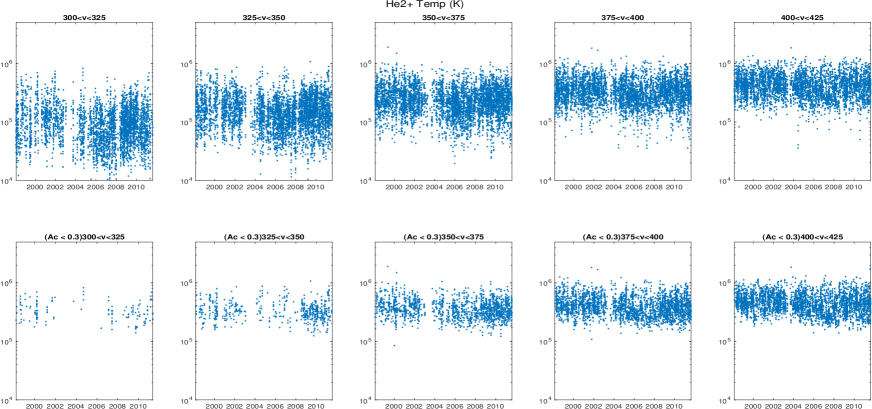
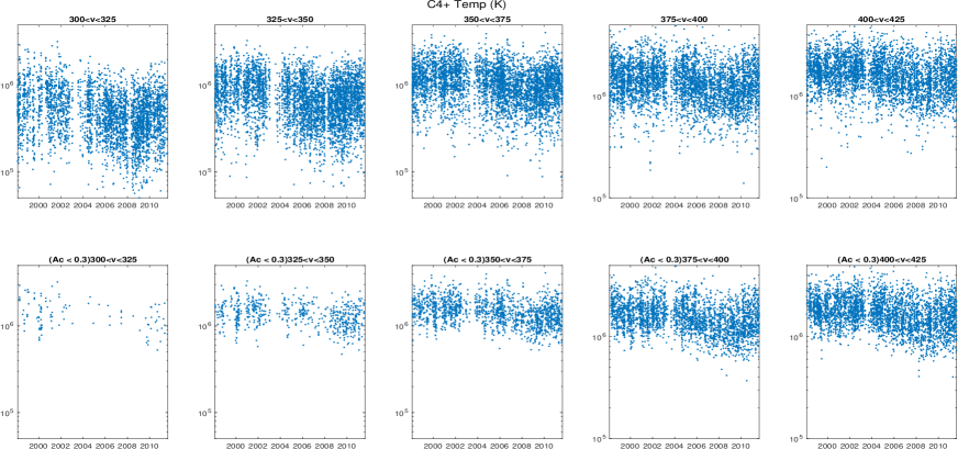
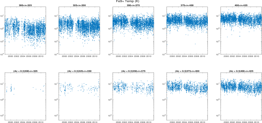
Figure 21: Comparison of ion temperatures at low speeds in collisionally young wind and the complete data set. First two rows: He${2+}$, middle two rows: C${4+}$, bottom tworows: Fe⁹⁺. For each ion, the general data set is shown on top, and the collisionally young data set is shown on bottom.

Figure 21 shows the effect of removing all collisionally old data from the sample, for a few representative ions: He²⁺, C⁴⁺ and Fe⁹⁺. Only speeds bins slower than 425 km s^-1are shown, to better illustrate the effects of Coulomb collisions; for each of the ions, the top row shows all the data in the bin, and the bottom row only the collisionally young plasma parcels.

Figure 21 shows three main results:

1. As expected, the slower the speed bin, the higher the density, so that increasingly less streams are collisionally young;

2. While the full dataset shows an overall large decrease of the ion temperatures as the speed of each bin decreases, the collisionally young data show very limited to no decrease in ion temperature;

3. In collisionally young velocity bins with enough surviving data, the dependence of the ion temperature on the solar cycle is preserved, indicating that it is likely not due to Coulomb collisions, but to a real process taking place in the solar wind.

4.6.2 Ion temperature vs charge-to-mass ratio and wind speed

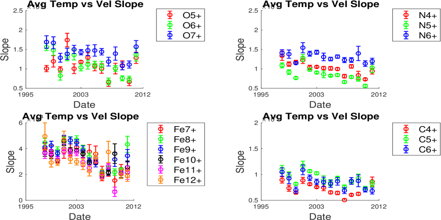
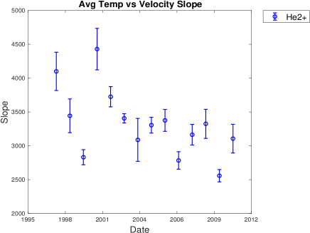
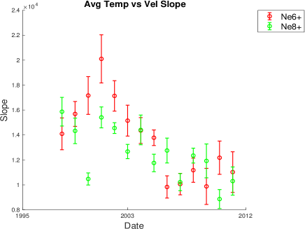
Figure 22: Same as Figure 14: values of $a_{lin}$ for the collisionally young wind.

The larger ion temperature values of low-speed, collisionally young plasma question the results obtained fitting a linear relationship between ion temperature and speed to the full dataset. Also, the relationship between ion temperature and the Z/A ratio may change. We have repeated those fits using only the collisionally young plasma. Figure 22 shows that the slope $a_{lin}$ of the linear fit between $T_{ion}$ and wind speed is:

1. shallower for all ions, consistently with slower wind having higher $T_{ion}$ values;

2. maintaining the same trend as a function of the solar cycle as the complete dataset, being lower at minimum and higher at maximum;

Thus, although the values of $a_{lin}$ change, the overall solar cycle dependence determined with the full dataset is preserved also for the collisionally young one.

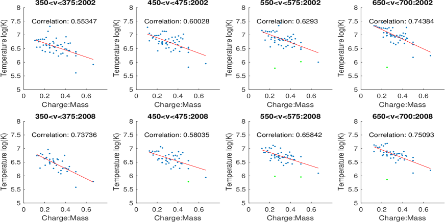
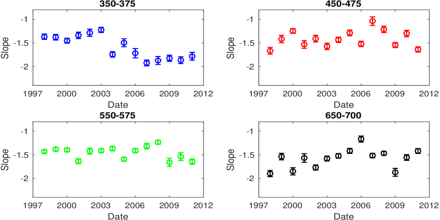
Figure 23: Same as Figure 15: values of $a_{Z/A}$ for the collisionally young wind.

As fas as the slope $a_{Z/A}$ of the linear fit between $\log T_{ion}$ and Z/A, results are shown in Figure 23. We find that $a_{Z/A}$ is:

1. unchanged at larger speeds (as expected);

2. less steep at lower speed, and with the same scatter as the other speed bins;

3. having approximately the same value in all speed bins;

4. uncorrelated to the solar cycle.

These results indicate that the process generating a dependence of the ion temperature on the Z/A ratio is the same for all wind speeds, and does not change along the solar cycle.

5 Discussion

5.1 Plasma density and wind ionization properties

The long-term decrease of solar wind proton density, visible at all speeds except the slowest bins, does not seem to correlate with the solar cycle. Such a decrease has an unknown origin; Zerbo & Richardson (2015) showed that 27-day proton density averages of the ecliptic solar wind started this decrease around 1990, and on longer timescales (dating back to the late 1960s) proton density changed slowly with timescales longer than 40 years. Also, we find that the proton density decrease does not affect the well known density-vs-velocity relationship: a double-sloped linear fit of yearly averages of the proton density with speed shows little variability, indicating that the measured density decreased affects all winds in the same way.

This slow, cycle-unrelated density variation should result in a gradual decrease of both ionization and recombination rates due to free electron-ion collisions, as the overall density of free electrons follows the proton density. In turn, decreased ionization and recombination should lead to freeze-in heights increasingly closer to the Sun and to lower wind ionization. Furthermore, as for the proton density, these changes should not show a clear correlation with the 11-year solar cycle. On the contrary, the present results confirm the findings of Lepri et al. (2013), who noted that the plasma charge state distribution closely tracks the solar cycle, being lower at minimum, and increasing together with the sunspot number. Most importantly, both the present results and the Lepri et al. (2013) results point towards an increase in wind ionization after 2010, contrarily to the expectations from the ongoing decrease of the electron density. This means that electron density is not the only cause of wind ionization evolution.

Landi & Lepri (2015) attempted to explain the charge state variations with photoionization from solar EUV and X-ray radiation outside flares, as EUV and X-ray fluxes are mostly emitted by active regions and depend critically on the solar cycle. Landi & Lepri (2015) found that photoionization indeed induces some variability, but it was insufficient to explain the measured variation in charge state ratios. Landi (2022, in preparation) added flare photoionization to the picture, but found that flare-enhanced high-energy photoionizing flux could not account for the missing, cycle dependent ionization. Cycle-related changes of plasma density and temperature in quiescent streamers, which might be responsible for ionization variations at least in the slow solar wind, were ruled out by Landi & Testa (2014) using remote sensing observations. Systematic measurements of density, temperatures and emission measures in equatorial coronal holes – the source of a large fraction of the fast speed wind observed by ACE – were carried with SDO/AIA from 2010 to 2019 encompassing most of cycle 24, and they also showed no significant variation along the solar cycle (Heinemann et al. 2021). Thus, the reason behind the solar cycle variation of wind ionization, which affects all elements, is still unclear.

Wind ionization is determined by plasma electron temperature, electron density, and speed. The first two quantities determine the local collisional ionization and recombination rates at any location along the wind trajectory, while speed determines the time spent by a wind plasma parcel at each location. Since electron density and temperature seem not to be the cause of the observed ionization variations, the only remaining possibility seems to be wind acceleration close to the Sun. In order to cause lower ionization at solar minimum, plasma speed needs to be faster close to the Sun, so that the solar wind spends less time in the densest and hottest part of the corona. This means that solar wind acceleration needs to be more efficient close to the Sun during solar minimum and less efficient at solar maximum. However, no independent confirmation of this scenario is currently available with remote sensing measurements.

Wind ionization models rely on ionization and recombination rates calculated using a Maxwellian distribution of electron velocity. Tails of high-energy electrons can significantly increase ionization rates, leading to a higher wind charge states (Cranmer 2014): in case their presence and size depended on the solar cycle, they could account for the observed cycle variations of wind ionization. Unfortunately, these high-energy electron populations have not yet been unambiguously identified by remote sensing observations.

5.2 Plasma fractionation processes: absolute and relative elemental abundances

Elemental abundances open a window on the evolution of the FIP effect along the solar cycle, which is largely unavailable from remote sensing observations due to the lack of a comprehensive and continuous monitoring of the solar corona with spectrally resolved data.

5.2.1 Absolute abundances

The variability of absolute abundances indicates a change in the capability of wind acceleration mechanisms to extract heavier ions over protons from the wind’s source region. The present results indicate that the composition of the slow solar wind is sensitive to the solar cycle, with the amount of heavy ions present in this wind being lower during solar minumum relative to solar maximum. This result affects all elements, including Oxygen, usually assumed to track Hydrogen’s response to ponderomotive forces, and confirms the results obtained by Lepri et al. (2013). At faster speeds such a solar cycle dependence is much reduced.

These results may be due to two different scenarios. First, the decreasing amount of change in composition as the wind speed approaches 500 km s^-1 is consistent with a ”two-wind scenario” where a coronal hole-associated wind is present at all speeds whose metallicity is weakly affected by the solar cycle, and a reconnection-driven slow wind is present at speeds lower than 500 km/s, which comes from initially closed magnetic structures and whose metallicity is lower at solar minimum. The decreasing amount of solar cycle dependence as speed approaches 500 km/s may be simply due to a decreasing fraction of wind originating from closed loop structures.

Second, if the observed FIP effect variations are due to the slow wind component coming from formerly closed loops, the present results may also suggest a marked change in the FIP fractionation occurring in closed magnetic structures as the solar cycle unfolds, which does not occur in open field lines.

The open question is to what extent can the FIP variation in the slow wind be ascribed only to a varying mixture in the wind source region, or to variability in the closed loops before their opening by reconnection, or both.

5.2.2 Relative elemental abundances

Similar results are found when relative abundances are considered. In fact, the FIP bias of the fast wind is largely constant and ranges between 1 and 1.5, consistently with model predictions (Laming 2015). Slow wind FIP bias, on the contrary, decreases during solar minimum, at which time the relative abundances in the slow wind resemble those in the fast wind.

As for the absolute abundances, this result is also consistent with the two-wind scenario, and it further suggests that coronal-hole associated wind dominates at all speeds during minimum, and that the fractionation process in its source region (coronal holes) is relatively stable during the solar cycle. At solar maximum slow wind coming from closed loop structures, whose FIP bias can even exceed 10, becomes prevalent at slow speeds. Thus, the variability in slow wind FIP fractionation may again be due either to an evolving mixture of source regions, or to a changing effectiveness of FIP fractionation in closed loops, or both.

Looking at individual abundance ratios, the relative C/O abundance is remarkably stable along the solar cycle at all speeds, indicating that the process that increases its value from the photospheric value of 0.45-0.55 to the measured $\approx$0.7 does not change in time. According to the ponderomotive force model (Laming 2015 and references therein) the $\approx$1.3-1.6 enhancement in the C/O ratio from open magnetic flux tubes in coronal holes can be due to slow-mode wave amplitudes of around 6.0 km s^-1. The stability of this ratio in time indicates that this process is not affected by the solar cycle, and its uniformity over all velocity ranges suggests that it is ubiquitous in all source regions of the solar wind, even if the measured C/O ratio enhancement is slightly larger than predicted for closed loop structures. The stability of this ratio in time argues for a scenario where the varying abundances in the slow wind are only due to a changing mixture of source regions at different phases of the solar cycle.

The relative Fe/C abundance, which can be taken as a proxy for the low-FIP/high-FIP relative abundance, shows two interesting results. First, its value ranges over a much larger span in the slow wind than in the faster wind, as shown in the upper row of Figure 7. This is again consistent with the ”two-wind” scenario, and indicates that the relative abundance of wind released from closed coronal structures decreases as the wind speed increases, thus decreasing the spread of FIP bias values measured in the solar wind.

Second, the Fe/C FIP bias changes with the solar cycle at all speeds, although the amount of change is lower for the faster wind streams. This result confirms the finding of McIntosh et al. (2011), which found that the Fe/O ratio, another proxy for the FIP effect in the solar wind, also shows some degree of variability in the fast wind during the decay phase of the solar cycle from 2005 to 2009. Further remote sensing observations of the sun-as-a-star by Brooks et al. (2017, 2018) also indicate that during the rising phase of the solar cycle (2010-2014) the FIP bias changes with time: their measurements mostly reflect the composition of the denser quiet Sun and active region plasmas where the reconnection-based slow wind likely comes from. Furthermore, despite the uncertainties in its measurement, the abundance of Ne seems to increase during solar minimum relative to all other elements, and the amount of increase seems to be lower at larger speeds. The present results for the Ne/O ratio confirm those already found by Shearer et al. (2014), and discussed by Landi & Testa (2015) considering also remote sensing observations.

It is interesting to note that Ne has the largest FIP value of all elements (21.6 eV), followed by Oxygen and Hydrogen (13.6 eV), Carbon (11.3 eV) and Iron (7.9 eV). The present results seem to indicate that solar cycle-induced FIP effect changes are visible in abundance ratios among elements with large FIP differences, such as Fe/C or Ne/X (X being all other heavy elements), and not in ratios between elements with a similar FIP value (such as C/O).

The variability of the low-FIP to high-FIP ratios in both the in-situ and remote sensing observations indicate that FIP fractionation processes indeed somehow change their effectiveness during the solar cycle. The increase in the Ne/O ratio confirms this result, as Ne is predicted to be depleted relative to all other elements with lower FIP (including the high FIP C, N, O and H).

Thus, the present results show that the solar cycle affects solar wind composition in two main ways:

1. By changing the relative abundances of elements with large FIP differences, indicating a changing effectiveness of FIP fractionation processes in all types of wind and thus in all of their source regions; and

2. By varying the relative importance of open versus closed magnetic field structures in the mixture of source regions for the solar wind slower than 500 km/s.

5.3 Heating and acceleration processes: ion temperatures and differential velocities

Preferential heating and acceleration of heavy ions over protons have been long observed in all types of solar wind, both in situ and close to the Sun.

Remote sensing observations from UVCS (Kohl et al. 1995) have shown that O⁶⁺ flows faster than Hydrogen, and exhibits a remarkably anisotropic temperature distribution where the perpendicular temperature is much larger than the neutral Hydrogen one (Kohl et al. 2006). These features start to be detectable in the inner solar corona, beyond 2 solar radii.

Preferential heavy ion heating has also long been identified in in-situ observations of the solar wind, with $T_{ion}/T_{p}$ ratios found to be approximately proportional to mass except in the densest streams (Bochsler 2007 and references therein). Berger et al. (2011) systematically studied ACE/SWICS measurements of heavy ion-proton differential speeds finding that most ions travel within $\pm 0.15~{}C_{A}$ (where $C_{A}$ is the Alfven speed) of the $\alpha$ speed, which in turn is significantly faster than the proton speed, confirming measurements of differential speeds found in less systematic measurements by a number of earlier authors. Duruvcova et al. (2017) further noted that 1) Helios and WIND measurements of $\alpha$-proton differential speeds are larger in faster winds; they decrease with distance from the Sun, a trend also found by Reisenfeld et al. (2001) to occur in Ulysses measurements up to more than 4 AU, and are qualitatively the same at solar minimum and solar maximum.

The present work adds a new temporal dimension to our determination of ion heating and acceleration. In fact, our results show that ion and proton temperatures follow three interesting trends:

1. Their absolute values seem to decrease during solar minimum, although the amount of decrease depends on speed itself;

2. The rate of increase of ion temperatures with speed also changes in time, being smaller during solar minimum as shown in Figure 14. These two results indicate that the ion temperatures of the fast wind decrease more than those in the slow wind during solar minimum.

3. The dependence on the ion temperatures on the Z/A ratio, and of the proton-ion temperature ratios on mass, on the contrary, is remarkably constant with time.

These results apply both to the general dataset and to the collisionally young one, although the slope of the $T_{ion}$ vs speed linear dependence is lower than for the full dataset due the higher $T_{ion}$ values of collisionally young wind at slow speeds. Also, once the effects of Coulomb collisions are minimized, all winds at any speed show the same dependence on Z/A.

The differential velocity results are much more ambiguous due to the paucity of data, which forced us to lose velocity resolution, and still have a limited number of data points. Also, it was not possible to determine whether collisionally young plasma streams from the slow wind have the same differential speed as those in the fast wind, as suggested by Stakhiv et al. (2016). Still, we could determine that the solar cycle did not affect much the differential speed between Hydrogen and all other elements, confirming the results of Duruvcova et al. 2017 and extending them to all heavy ions.

The origin of ion preferential heating and acceleration has been long studied (see the reviews of Marsch 2006 and Verscharen et al. 2019). Both phenomena have been linked to the action of waves as two sides of the same coin. For example, Isenberg & Hollweg (1982) linked preferential ion acceleration to the same Alfven wave dissipation term also responsible for ion preferential heating; further refinements involving Alfven wave ion cyclotron resonant heating were later discussed by Hollweg & Isenberg (2002). Other proposed avenues for ion heating are high-frequency Alfven wave turbulence (Coleman 1968), and more recently stochastic heating by low-frequency Alfven wave turbulence (Chandran 2010, Chandran et al. 2010, 2013). In all cases, magnetic field fluctuations play a central role in the preferential heating and acceleration of coronal ions into the solar wind over a range of distances from the Sun.

The present results indicate that the effectiveness of these processes does change with time. However, results are quite nuanced. The decrease in the absolute value of the ion temperatures at all speeds indicates that perpendicular heating has been weaker during the minimum phase of cycle 24, pointing towards a weakening of the heating processes both for protons and for heavier ions at all speeds; also, the decrease of effectiveness has been more marked in the fast wind than in the slow wind.

On the other hand, the nature of the process causing preferential heating and acceleration of heavy ions relative to protons seems to have remained the same. In fact, not only is there no clear hint at a decrease of differential ion-proton velocity, but the dependence of the ion temperature values on Z/A, and the mass proportionality of ion-to-proton temperature ratios are unchanged for all ions at any speed over the entire 1998-2011 period covered by the present study.

If wave-particle interactions are responsible for both proton and ion heating, and for preferential ion heating and acceleration, our results seem to point towards a weakening of these interactions. This may be due to a decrease during the last solar minimum of the wave energy available to heat and accelerate the solar wind, which would track the decrease in magnetic field strength both in the solar wind (Zerbo & Richardson 2015) and in the photosphere (Ingale et al. 2019 and references therein). Still, there are no remote sensing confirmation of such a decrease in the solar corona where heating and acceleration take place. Such a variation could in principle be observable through cycle-related changes in the width of spectral lines observed in the solar atmosphere, although such measurements are difficult to make due to the lack of systematic spectroscopic observations, to line-of-sight effects, and to the presence of two distinct contributions (ion thermal and non-thermal speeds) into one single observable (spectral line widths). Past attempts at determining cycle-related variations of non-thermal motions (Harra et al. 2015), as well as ion temperatures (Landi 2007) have found no change, although they were carried out only over limited portions of the solar cycle.

6 Conclusions

The solar wind is intrinsically a cycle-dependent phenomenon. In the present work, we have extended this conclusion to the signatures of electron-ion interactions (wind ionization), elemental abundances, and wave-based heating and acceleration (ion temperatures, differential velocity); where possible, we tried to minimize the effect of Coulomb collisions on the latter signatures, and investigate whether more pristine wind properties change with the solar cycle. We also further refined the velocity resolution of our measurements over previous studies. The present work clearly shows that all wind properties do change with the solar cycle; specifically

1. Both proton density and temperature show a significant time dependence, but while temperature variations clearly follow the 11-year solar cycle, proton density shows a steady decline spanning longer timescales with no apparent periodic behavior;

2. Both absolute and relative elemental abundances change as a function of the solar cycle, with the effects being more pronounced in the slow wind than in the fast wind;

3. Ion temperatures decrease their absolute value during the 2008 solar minimum and begin to recover afterwards; their dependence on wind speed is affected, but their dependence on the Z/A ratio and on ion mass does not change with time;

4. Proton-ion differential speeds are different between the wind slower than 400 km s^-1(being almost zero) and the wind faster than 550 km s^-1(where they range between 20-70 /kms), but they do not change with time;

5. Charge state distribution and charge state ratios (including those of Fe) are strongly dependent on the cycle phase, being lower during solar minimum;

6. Collisionally young wind shows higher ion temperatures at low speed, but its dependence on mass, Z/A ratio, wind speed and time along the solar cycle does not change.

While the decrease of proton density seems to act on longer timescales than the solar cycle, the other plasma properties we investigated do show a clear dependence on the 11-year solar cycle. Our results point towards the scenario proposed by Stakhiv et al. (2016), where both the slow wind and the fast wind are accelerated by magnetic waves, but originate from different structures, whose relative importance decreases as wind speed increases: the fast wind is present at all speeds, originating from open field structures, while the slow wind comes from the reconnection-based opening of closed loops and is absent at speeds larger than $\approx$500 km s^-1. Our work adds to this scenario three new features:

1. The relative importance of open field versus closed field sources in the slow wind changes with the solar cycle, with the latter greatly decreasing in importance during solar minimum;

2. The signatures of wave-based heating and acceleration, shown by proton and ion temperatures, and differential velocities, are present throughout the solar cycle and indicate that such a process is always active;

3. The effectiveness of magnetic waves at heating and accelerating the solar wind, as well as shaping its elemental composition, is lower during solar minimum.

There are several open questions that still need to be answered. The origin of the long-term decrease of the proton density is not clear, and also the large variations in the solar wind charge state distribution can not be explained neither by a decrease of electron density and temperature in the solar wind in the inner corona, nor by the cycle-related variations of EUV and X-ray wind photoionization. Furthermore, ACE/SWICS could only sample the solar wind at the ecliptic, whose fast component seldom exceeds speeds of 700 km s^-1: on the contrary, Ulysses showed that out of the ecliptic the wind is faster, with a speed that clusters around 750 km s^-1. Most of this wind, as well as the solar cycle dependence of its properties still remain to be studied. Also, more details are needed in our understanding of the dependence of differential speed on both speed and cycle phase, due to the paucity of the data sample we have utilized. Hopefully the instruments on board Solar Orbiter (both in-situ and remote sensing) will help in answering some of these questions.

7 References

1. Berger, L., Wimmer-Schweingruber, R.F., & Gloeckler, G. 2011, Phys. Rev. Lett., 106, 151103

2. Berteaux, J.L., Kyrölä, E., Quemerais, E., et al. 1995, Sol. Phys., 162, 403

3. Bochsler, P. 2007, Astr. Astroph. Rev., 14, 1

4. Brooks, D.H., Baker, D., van Driel-Gesztelyi, L., & Warren, H.P. 2017, Nature Comm., 8, 183

5. Brooks, D.H., Baker, D., van Driel-Gesztelyi, L., & Warren, H.P. 2018, ApJ, 861, 42

6. Cane, H.V., & Richardson, I.G. 2003, JGR, 108, 1156

7. Chandran, B.D.G. 2010, ApJ, 720, 548

8. Chandran, B.D.G., Li, B., Rogers, B., et al. 2010, ApJ, 720, 503

9. Chandran, B.D.G., Verscharen, D., Quataert, E. et al. , 2013, ApJ, 776, 45

10. Coleman, P.J. Jr 1968, ApJ, 153, 371

11. Cranmer, S.R., Field, G.B., & Kohl, J.L. 1999, ApJ, 518, 937

12. Cranmer, S.R., Panasyuk, A.V., & Kohl, J.L. 2008, ApJ, 678, 1480

13. Cranmer, S.R. 2014, ApJ 791, L31

14. Duruvcova, T., Safrankova, J., Nemecek, Z., & Richardson, J.D. 2017, ApJ, 850, 164

15. Finley, A.J., Matt, S.P., & See, V. 2018, ApJ, 864, 125

16. Fludra, A. 2015, ApJ, 803, 66

17. Gloeckler, G., Cain, J., Ipavich, F.M., et al. 1998, Sp. Sci. Rev., 86, 497

18. Harra, L., Baker, D., Edwards, S.J., et al. 2015, Sol. Phys., 290, 3203

19. Heber, V.S., Baur, H., Bochsler, P., et al. (2012), ApH, 759, 121

20. Hollweg, J.V., & Isenberg, P.A. 2002, JGR, 107, 1147

21. Ingale, M., Janardhan, P., & Bisoi, S.K. 2019, JGR, 124, 6363

22. Isenberg, P.A., & Hollweg, J.V. 1982, JGR, 87, 5023

23. Kasper, J.C., Stevens, M.L., Lazarus, A.J., Steinberg, J.T., & Ogilvie, K.W. 2007, ApJ, 660, 901

24. Kasper, J.C., Stevens, M.L., Korreck, K.E., et al. 2012, ApJ, 745, 162

25. Kasper, J.C., Bennett, M.A., Stevens, M.L., & Zaslavsky, A. 2013, Phys. Rev. Lett., 110, 091102

26. Khabibrakhmanov, I.K. & Mullan, D.J. 1994, ApJ, 430, 814

27. Kohl, J.L., Esser, R., Gardner, L.D., et al. 1995, Sol. Phys., 162, 313

28. Kohl, J.L., Noci, G., Cranmer, S.R., & Raymond, J.C. 2006, Astr. Astroph. Rev., 13, 31

29. Laming, M.J. 2015, Living Reviews Solar Physics, 12, 2

30. Lamy, P., Floyd, O., Quemerais, E., Boclet, B., & Ferron, S. 2017, J. Geoph. Res., 122, 50

31. Landi, E. 2007, ApJ, 663, 1363

32. Landi, E., & Testa, P. 2015, ApJ, 800, 110

33. Landi, E., & Testa, P. 2014, ApJ, 787, 33

34. Landi, E., & Lepri, S.T. 2015, ApJ, 812, 28

35. Landi, E., Alexander, R.L., Gruesbeck, J.R., et al. 2012, ApJ, 744, 100

36. Landi, E. & Cranmer, S.R. 2009, ApJ, 691, 794

37. Lepri, S.T., Landi, E., & Zurbuchen, T.H. 2013, ApJ, 768, 94

38. Luhmann, J.G., Li, Y., Arge, C.N., Gazis, P.R., & Ulrich, R. 2002, JGR, 107, 1154

39. Marsch, E. 2006, LRSP, 3, 1

40. McComas, D.J., Ebert, R.W., Elliott, H.A., et al. 1998, G. Geoph. Res., 35, L18103

41. McComas, D.J., Angold, N., Elliott, H.A., et al. 2013, ApJ, 779, 2

42. McIntosh, S.W., Kiefer, K.K., Leamon, R.J., Kasper, J.C., & Stevens, M.L. 2011, ApJL, 740, L23

43. Owens, M.J., Cliver, E., McCracken, K.G. et al. 2016, J. Geoph. Res., 121, 6048

44. Reisenfeld, D.B., Gary, S.P., Gosling, J.T., et al. 2001, JGR, 106, 5693

45. Richardson, I.G., & Cane, H.V. 2010, Sol. Phys., 264, 189

46. Shearer, P., von Steiger, R., Raines, J.M., et al. 2014, ApJ, 789, 60

47. Smith, C.W., L’Hereux, J., Ness, N.F., et al. 1998, Sp. Sci. Rev., 86, 613

48. Tracy, P.J., Kasper, J.C., Zurbuchen, T.H., et al. 2015, ApJ, 812, 170

49. Tracy, P.J., Kasper, J.C., Raines, J.M., et al. 2016, Phys. Rev. Lett., 116, 255101

50. Verscharen, D., Klein, K.G., & Maruca, B.A. 2019, LRSP, 16, 5

51. Yamauchi, Y., Suess, S.T., Steinberg, J.T., & Sakurai, T. 2004, JGR, 109, A03104

52. Yermolaev, Y.I., Lodkina, I.G., Khokhlachev, A.A., et al. 2021, JGR, 126, e2021JA029618

53. Wang, Y.-M., 1998, ASP Conf. Series, 154, 131

54. Zerbo, J.-L. & Richardson, J.D. 2015, J. Geoph. Res., 120, 10250