Graphical mean curvature flow with bounded bi-Ricci curvature

Abstract.

We consider the graphical mean curvature flow of strictly area decreasing maps $f:M\to N$, where $M$ is a compact Riemannian manifold of dimension $m>1$ and $N$ a complete Riemannian surface of bounded geometry. We prove long-time existence of the flow and that the strictly area decreasing property is preserved, when the bi-Ricci curvature $\operatorname{BRic}_{M}$ of $M$ is bounded from below by the sectional curvature $\sigma_{N}$ of $N$. In addition, we obtain smooth convergence to a minimal map if $\operatorname{Ric}_{M}\geq\sup\{0,{\sup}_{N}\sigma_{N}\}$. These results significantly improve known results on the graphical mean curvature flow in codimension $2$.

1. Introduction and summary

Suppose $f:M\to N$ is a smooth map between the Riemannian manifolds $M$ and $N$ and let

$$\varGamma_{f}:=\big{\{}(x,f(x))\in M\times N:x\in M\big{\}}$$

denote the graph of $f$. We deform $\varGamma_{f}$ by the mean curvature flow. Some general questions are whether the flow stays graphical, it exists for all times, and it converges to a minimal graphical submanifold $\varGamma_{\infty}$ generated by a smooth map $f_{\infty}:M\to N$. In this case, $f_{\infty}$ is called a minimal map and can be regarded as a canonical representative of the homotopy class of $f$.

The first result concerning the evolution of graphs by its mean curvature was obtained by Ecker and Huisken [ecker]. They proved long-time existence of the mean curvature flow of entire graphical hypersurfaces in the euclidean space and convergence to flat subspaces under the assumption that the graph is straight at infinity. For maps between arbitrary Riemannian manifolds the situation is more complicated. However, under suitable conditions on the differential of $f$ and on the curvatures of $M$ and $N$, it is possible to establish long-time existence and convergence of the graphical mean curvature flow; for example see [lubbe1, ss2, ss1, ss0, stw, tsuiwang, wang].

A smooth map $f:M\to N$ between Riemannian manifolds is called strictly area decreasing, if

$$|df(v)\wedge df(w)|<|v\wedge w|,\text{ for all }v,w\in TM.$$

One of the first results for the graphical mean curvature flow in higher codimension was obtained by Tsui and Wang [tsuiwang], where they proved that each initial strictly area decreasing map $f:\mathbb{S}^{m}\to\mathbb{S}^{n}$ between unit spheres of dimensions $m,n\geq 2$ smoothly converges to a constant map under the flow. This result has been generalized much further by other authors; see for instance [ss2, ss0]. In [ss2] we proved that the mean curvature flow smoothly deforms a strictly area decreasing map $f:M\to N$ into a constant one, if $M$ and $N$ are compact, the Ricci curvature $\operatorname{Ric}_{M}$ of $M$ and the sectional curvatures $\sigma_{M}$ and $\sigma_{N}$ of $M$ and $N$, respectively, satisfy

$$\sigma_{M}>-\sigma\quad\text{and}\quad\operatorname{Ric}_{M}\geq(m-1)\sigma\geq(m-1)\sigma_{N}$$ (O)

for some positive constant $\sigma>0$, where $m$ is the dimension of $M$. Optimal results were obtained in [ss0] for area decreasing maps between surfaces.

We consider area decreasing maps $f:M\to N$, where $M$ is compact and $N$ is a complete surface $N$ with bounded geometry, that is the curvature of $N$ and its derivatives of all orders are uniformly bounded, and the injectivity radius is positive. In order to state our main results, we need to introduce some curvature conditions.

Definition 1.1.

Let $(M,{\operatorname{g}_{M}})$ be a Riemannian manifold of dimension $m>1$ and let $(N,{\operatorname{g}_{N}})$ be a Riemannian surface. For any pair of orthonormal vectors $v,w$ on $M$, the bi-Ricci curvature $\operatorname{BRic}_{M}$ is given by

$${\operatorname{BRic}}_{M}(v,w)=\operatorname{Ric}_{M}(v,v)+\operatorname{Ric}_{M}(w,w)-\sigma_{M}(v\wedge w),$$

where $\operatorname{Ric}_{M}$ is the Ricci curvature and $\sigma_{M}$ the sectional curvature of $M$.

1. We say that the curvature condition (A) holds, if the bi-Ricci curvature of $M$ is bounded from below by the sectional curvature of $N$, that is if ${\operatorname{BRic}}_{M}\geq{\sup}_{N}\sigma_{N}$.

2. We say that the curvature condition (B) holds, if the Ricci curvature of $M$ is non-negative.

3. We say that the curvature condition (C) holds, if the Ricci curvature of $M$ is bounded from below by the sectional curvature of $N$, that is if $\operatorname{Ric}_{M}\,\geq\,{\sup}_{N}\sigma_{N}$.

The concept of bi-Ricci curvature was introduced by Shen and Ye [shen]. Note that the condition (C) implies (B) if ${\sup}_{N}\sigma_{N}\geq 0$ and that (B) implies (C) if ${\sup}_{N}\sigma_{N}\leq 0$. In particular, conditions (B) and (C) are equivalent if ${\sup}_{N}\sigma_{N}=0$. We will discuss these conditions in detail in Remark 2.2.

Our main results are stated in Theorems A, F and its corollaries which are presented in Section 2. Roughly speaking, in Theorem A we obtain long-time existence of the mean curvature flow of area decreasing maps under the condition (A) and convergence to minimal maps under the conditions (A), (B), and (C). The proof of Theorem A relies on an estimate for the mean curvature of the evolving submanifolds and a Bernstein type theorem for minimal graphs. The classification of these minimal maps will be presented in Theorem F. The proofs of Theorems A and F are given in Section 6.

2. Long-time existence and convergence of the flow

The main results for the mean curvature flow are stated below.

Theorem A.

Let $(M,{\operatorname{g}_{M}})$ be a compact Riemannian manifold of dimension $m>1$ and let $(N,{\operatorname{g}_{N}})$ be a complete Riemannian surface of bounded geometry. Suppose $f_{0}:M\to N$ is strictly area decreasing.

1. If the curvature condition (A) holds, that is $\operatorname{BRic}_{M}\geq{\sup}_{N}\sigma_{N}$, then the induced graphical mean curvature flow exists for $t\in[0,\infty)$, and the evolving maps $f_{t}:M\to N$ remain strictly area decreasing for all $t$.

2. If the curvature conditions (A) and (B) hold, that is $\operatorname{BRic}_{M}\geq{\sup}_{N}\sigma_{N}$ and $\operatorname{Ric}_{M}\geq 0$, then $\{f_{t}\}_{t\in[0,\infty)}$ is uniformly bounded in $C^{1}(M,N)$ and remains uniformly strictly area decreasing.

3. If the curvature conditions (A) and (C) hold, that is $\operatorname{BRic}_{M}\geq{\sup}_{N}\sigma_{N}$ and $\operatorname{Ric}_{M}\geq{\sup}_{N}\sigma_{N}$, then the mean curvature stays uniformly bounded. If $\{f_{t}\}_{t\in[0,\infty)}$ is uniformly bounded in $C^{1}(M,N)$, then $\{f_{t}\}_{t\in[0,\infty)}$ is uniformly bounded in $C^{k}(M,N)$, for all $k\geq 1$.

4. Suppose that the curvature conditions (A), (B) and (C) hold, that is we have $\operatorname{BRic}_{M}(v,w)\geq{\sup}_{N}\sigma_{N}$ and $\operatorname{Ric}_{M}(v,v)\geq\max\{0,{\sup}_{N}\sigma_{N}\}$. Then we get the following results:

   1. $\{f_{t}\}_{t\in[0,\infty)}$ is uniformly bounded in $C^{k}(M,N)$, for all $k\geq 1$.

   2. In the following cases $\{f_{t}\}_{t\in[0,\infty)}$ is uniformly bounded in $C^{0}(M,N)$:

      1. $\operatorname{Ric}_{M}>0$.

      2. $N$ is compact.

      3. ${\sup}_{N}\sigma_{N}\leq 0$ and $N$ is simply connected.

      4. ${\sup}_{N}\sigma_{N}\leq 0$ and $N$ contains a totally convex subset $\mathscr{C}$; that is $\mathscr{C}$ contains any geodesic in $N$ with endpoints in $\mathscr{C}$.

      5. There exists $c\in{\mathbb{R}}$ and a smooth function $\psi:N\to{\mathbb{R}}$ such that $\psi$ is convex on the set $N^{c}:=\{y\in N:\psi(y)<c\}$, $\overline{N^{c}}$ is compact and $f_{0}(M)\subset N^{c}$.

   3. Under the assumption that the family $\{f_{t}\}_{t\in[0,\infty)}$ is uniformly bounded in $C^{k}(M,N)$, for all $k\geq 0$, the following holds:

      1. There exists a subsequence $\{f_{t_{n}}\}_{n\in{\mathbb{N}}}$, $\lim_{n\to\infty}t_{n}=\infty$, that smoothly converges to one of the minimal maps classified in Theorem F.

      2. If there exists a subsequence $\{f_{t_{n}}\}_{n\in{\mathbb{N}}}$ of the family $\{f_{t}\}_{t\in[0,\infty)}$ that converges in $C^{0}(M,N)$ to a constant map, then the whole flow $\{f_{t}\}_{t\in[0,\infty)}$ smoothly converges to this constant map.

      3. If there exists a point $x\in M$ such that $\operatorname{Ric}_{M}(x)>0$, then the flow $\{f_{t}\}_{t\in[0,\infty)}$ smoothly converges to a constant map.

      4. If $(M,{\operatorname{g}_{M}})$ and $(N,{\operatorname{g}_{N}})$ are real analytic, then the flow smoothly converges to one of the minimal maps classified in Theorem F.

Let us discuss now some interesting corollaries of Theorem A.

Corollary B.

Let $M$ be a compact manifold with non-vanishing Euler characteristic $\chi(M)$, and let $N$ be a compact Riemann surface of genus bigger than one.

1. If $M$ is Kähler with vanishing first Chern class $c_{1}(M)$, then any smooth map $f:M\to N$ is smoothly null-homotopic.

2. More generally, the same result holds if $M$ admits a metric of non-negative Ricci curvature.

Proof.

(a) If $M$ is a Kähler manifold with vanishing first Chern class, then by a famous theorem of Yau [yau], $M$ admits a Ricci flat Kähler metric and this case can be reduced to part (b).

(b) Let ${\operatorname{g}_{M}}$ be a metric of non-negative Ricci curvature on $M$. Since $N$ has genus bigger than one, we can endow $N$ with a complete Riemannian metric $\operatorname{g}_{N}$ of constant negative curvature $\sigma_{N}$. Since $\dim N=2$, the map $f:M\to N$ has at most two non-trivial singular values $\lambda\geq\mu$ with respect to the metrics ${\operatorname{g}_{M}}$ and $g_{N}$. For a constant $r>0$ define the new metric $\operatorname{g}_{r}:=r^{2}\operatorname{g}_{N}$. Then the sectional curvature $\sigma_{r}$ of $\operatorname{g}_{r}$, and the singular values $\lambda_{r}$ and $\mu_{r}$ of $f$ with respect to ${\operatorname{g}_{M}}$ and $\operatorname{g}_{r}$ are given by $\lambda_{r}=r\lambda$, $\mu_{r}=r\mu$ and $\sigma_{r}=r^{-2}\sigma_{N}.$ If we choose $r$ sufficiently small, then $f$ will be strictly area decreasing with respect to ${\operatorname{g}_{M}}$, $\operatorname{g}_{r}$ and $\sigma_{r}$ will be so small that all curvature conditions in (A), (B) and (C) are satisfied. Applying the mean curvature flow to the graph $\varGamma_{f}$ of $f$ in $(M,{\operatorname{g}_{M}})\times(N,{\operatorname{g}_{N}})$, Theorem A(d) and Theorem F imply that $f$ is homotopic to a constant map if $M$ does not have vanishing Euler characteristic. ∎

Remark 2.1.

Most of the Calabi-Yau manifolds have non-vanishing Euler characteristic. For example, the Euler number of K3-surfaces is $24$. The statement in (b) cannot be extended to the case where $N$ is $\mathbb{S}^{2}$ or $\mathbb{T}^{2}$. Neither the Hopf fibration $f:\mathbb{S}^{3}\to\mathbb{S}^{2}$ nor the projections $\pi_{\mathbb{S}^{2}}:\mathbb{S}^{1}\times\mathbb{S}^{2}\to\mathbb{S}^{2}$, $\pi_{\mathbb{T}^{2}}:\mathbb{S}^{1}\times\mathbb{T}^{2}\to\mathbb{T}^{2}$ are homotopic to a constant map or to a geodesic.

Remark 2.2.

It is easy to construct examples of long-time existence but no convergence. Take $M=\mathbb{S}^{1}\times\mathbb{S}^{2}$ with the standard product metric and for $N$ choose $\mathbb{S}^{1}\times{\mathbb{R}}$ with a rotationally symmetric metric of negative curvature; see Figure 1(a). Then $\operatorname{Ric}_{M}\geq 0\geq\sigma_{N}$ and the condition (A) is satisfied. Fix $z_{0}\in{\mathbb{R}}$, let $c_{0}:\mathbb{S}^{1}\to N$ be the circle $c_{0}(s)=(s,z_{0})$ and define $f_{0}(s,p):=c_{0}(s)$, $(s,p)\in\mathbb{S}^{1}\times\mathbb{S}^{2}$. Clearly, $f_{0}$ is strictly area decreasing. The solution $f_{t}$ to the mean curvature flow will be of the form $f_{t}(s,p)=(s,z(t))$, where $z:[0,\infty)\to{\mathbb{R}}$ is a smooth function that becomes unbounded when $t\to\infty$. All conditions in Theorem A(d) are satisfied, except those in (2) guaranteeing $C^{0}$-bounds. However, the solution is uniformly bounded in $C^{k}(M,N)$ for all $k\geq 1$ and the mean curvature tends to zero in $L^{2}$ for $t\to\infty$. Nevertheless, there exist rotationally symmetric hyperbolic metrics on the cylinder for which we can apply Theorem A(d). For example, the closed geodesic $\mathscr{C}$ on the one-sheet hyperboloid depicted in Figure 1(b) is totally convex.

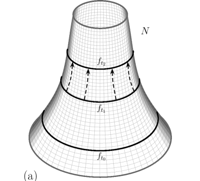
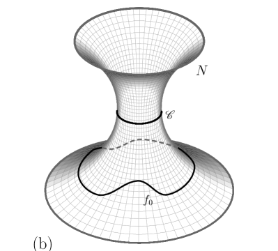
Figure 1. (a) Negatively curved surface without closed geodesics. (b) Negatively curved surface with a totally convex subset.

Remark 2.3.

We add some remarks concerning the curvature conditions and the results of Theorem A.

1. In dimensions $m=2,3$, the curvature condition (A) is equivalent to $\operatorname*{Scal}_{M}\geq\operatorname*{Scal}_{N},$ where these are the scalar curvatures of $M$ and $N$. Therefore, we recover the main results obtained in [ss0]. For $m=4$, (A) is equivalent to $\operatorname{Scal}_{M}-2\,{\sigma}_{M}(v\wedge w)\geq\operatorname*{Scal}_{N},$ for all $v,w\in TM.$

2. If $M$ and $N$ satisfy (A), then by taking traces at each point $x\in M$, the scalar and the Ricci curvatures of $M$ can be estimated by

   $$(m-3) \!\!\!\operatorname{Ric}_{M}(v,v)\!\!\!\! +\operatorname{Scal}_{M}\geq(m-1){\sup}_{N}\sigma_{N},$$ (2.1)

   $$\!\!\!{\operatorname*{Scal}}_{M}\!\!\!\!\!\!\!\!\!\!\!\!\!\! \geq\frac{m(m-1)}{2m-3}{\sup}_{N}\sigma_{N},$$ (2.2)

   and, for $m\neq 3$, equality occurs if and only if at $x$ all sectional curvatures of $M$ are equal. Thus, if $m\neq 3$ and at each $x\in M$ there exist at least two distinct sectional curvatures, then (A) can only be satisfied as a strict inequality.

3. The results in [ss2, ss1] were obtained under the assumption (O). It turns out that (O) implies (A) and, in particular, in this case (A) becomes even strict when $m>2$. Indeed, if $m=2$ the conclusion follows from $\operatorname{Ric}_{M}(v,v)=\operatorname{Ric}_{M}(w,w)$ for any $v,w\in TM$. In case $m>2$, it suffices to check this for an orthonormal frame $\{\alpha_{1},\dots,\alpha_{m}\}$ for which the Ricci tensor becomes diagonal. Then, for any $i\neq j$, we get

   $$\hskip 15.0pt\operatorname{BRic}_{M}(\alpha_{i},\alpha_{j}) \!\!\!=\!\!\! \operatorname{Ric}_{M}(\alpha_{i},\alpha_{i})+{\sum}_{k\neq j,i}\sigma_{M}(\alpha_{k}\wedge\alpha_{j})$$

   $$\!\!\!>\!\!\! (m-1)\sigma-(m-2)\sigma=\sigma\geq{\sup}_{N}\sigma_{N}.$$

   However, (A) does not imply (O), hence condition (A) is more general than (O). To obtain a better picture, let us assume that the sectional curvatures of $(M,{\operatorname{g}_{M}})$ are all constant to $\sigma_{M}$ and that the curvature of $N$ is given by a constant $\sigma_{N}$. The curvature condition (O) of [ss2] is then equivalent to $\sigma_{M}\geq\sigma_{N}$ and $\sigma_{M}>0.$ When the sectional curvatures are constant, (A), (B) and (C) are equivalent to (in this order):

   $$(2m-3)\sigma_{M}\geq\sigma_{N},\quad\sigma_{M}\geq 0\quad\text{and}\quad(m-1)\sigma_{M}\geq\sigma_{N}.$$

   Therefore, the results in Theorem A are stronger than those in [ss2].

Given a map $f:\mathbb{S}^{m}\to\mathbb{S}^{n}$ between unit spheres with singular values $\lambda_{1}\geq\lambda_{2}\geq\cdots\geq\lambda_{m}$, the number $\operatorname{Dil}_{2}(f)=\max\lambda_{1}\lambda_{2}$, is called the 2-dilation of $f$. An interesting question is to determine when such a map is homotopically trivial. In this direction, we obtain the following result.

Corollary C.

For the standard unit spheres $(\mathbb{S}^{m},\operatorname{g}_{\mathbb{S}^{m}})$ and $(\mathbb{S}^{2},\operatorname{g}_{\mathbb{S}^{2}})$ let us define

$$\mathcal{A}_{m-1}:=\{f\in C^{\infty}(\mathbb{S}^{m},\mathbb{S}^{2}):\operatorname{Dil}_{2}(f)<m-1\}.$$

Then for $m>1$ and for any $f_{0}\in\mathcal{A}_{m-1}$ there exists a smooth homotopy $\{f_{t}\}_{t\in[0,\infty)}\subset\mathcal{A}_{m-1}$ deforming $f_{0}$ into a constant map. This homotopy can be given by the mean curvature flow of $f_{0}$ as a map between $(\mathbb{S}^{m},\operatorname{g}_{\mathbb{S}^{m}})$ and the scaled $2$-sphere $(\mathbb{S}^{2},(m-1)^{-1}\operatorname{g}_{\mathbb{S}^{2}})$. In particular, $\mathcal{A}_{m-1}$ is smoothly contractible.

Proof.

Maps in $\mathcal{A}_{m-1}$ are strictly area decreasing maps from $(\mathbb{S}^{m},\operatorname{g}_{\mathbb{S}^{m}})$ to $(\mathbb{S}^{2},(m-1)^{-1}\operatorname{g}_{\mathbb{S}^{2}})$. The sectional curvature of ${\operatorname{g}_{N}}:=(m-1)^{-1}\operatorname{g}_{\mathbb{S}^{2}}$ is $m-1$ and the result follows from Remark 2.3(e), because in this case the curvature conditions in Theorem A are equivalent to $m-1\geq\sigma_{N}$. ∎

Remark 2.4.

It is well-known that the homotopy groups $\pi_{m}(\mathbb{S}^{2})$ are non-trivial for $m\geq 2$ and are finite for $m\geq 4$; see [berrick, curtis, gray]. Consequently, in Corollary C, we cannot increase the upper bound for $\operatorname{Dil}_{2}(f)$ arbitrarily without losing the contractibility of the corresponding set

$$\mathcal{A}_{m,c}:=\{f\in C^{\infty}(\mathbb{S}^{m},\mathbb{S}^{2}):\operatorname{Dil}_{2}(f)<c\}.$$

A natural problem arises; to determine the number

$$\mathfrak{c}_{m}:=\sup\{c>0:\mathcal{A}_{m,c}\text{ is smoothly contractible}\}.$$

The Hopf fibration $f:\mathbb{S}^{3}\to\mathbb{S}^{2}$ has constant singular values $\lambda_{1}=\lambda_{2}=2$ and $\lambda_{3}=0$. Moreover, it is minimal, but not totally geodesic, and not homotopic to a constant map; see [markellos, Remark 1]. Hence, from Corollary C we see that

$$2\leq\mathfrak{c}_{3}\leq 4\quad\text{ and }\quad m-1\leq\mathfrak{c}_{m}<\infty,$$

for $m>2$. Since the identity map $\operatorname*{Id}:\mathbb{S}^{2}\to\mathbb{S}^{2}$ is not homotopic to the constant map, we have that $\mathfrak{c}_{2}=1$.

In dimension three the results in Theorem A can be summarized in the following corollary.

Corollary D.

Let $(M,{\operatorname{g}_{M}})$ be a compact $3$-manifold and let $(N,{\operatorname{g}_{N}})$ be a complete surface of bounded geometry that satisfy the curvature condition

$$\operatorname{Ric}_{M}\geq\max\{0,{\sup}_{N}\sigma_{N}\}.$$

Then (A), (B) and (C) in Theorem A are satisfied and for any strictly area decreasing initial map $f_{0}:M\to N$ the results in Theorem A(d) apply.

Proof.

The conditions (B) and (C) hold by assumption. Since $m=3$, the condition (A) is equivalent to $\operatorname{Scal}_{M}\geq 2\,{\sup}_{N}\sigma_{N}.$ We distinguish two cases.

1. ${\sup}_{N}\sigma_{N}\geq 0$. In this case (C) $\Rightarrow\operatorname{Scal}_{M}\geq 3\,{\sup}_{N}\sigma_{N}\geq 2\,{\sup}_{N}\sigma_{N}$.

2. ${\sup}_{N}\sigma_{N}\leq 0$. In this case (B) $\Rightarrow\operatorname{Scal}_{M}\geq 0\geq{\sup}_{N}\sigma_{N}\geq 2\,{\sup}_{N}\sigma_{N}$.

Therefore, the curvature condition (A) holds and Theorem A applies. ∎

The next corollary follows from the Künneth formula and the fact that compact manifolds with positive Ricci curvature do not admit non-trivial harmonic $1$-forms. We give a proof using mean curvature flow.

Corollary E.

Let $M=L\times N$ be the product of a compact manifold $L$ and a compact surface $N$ of genus bigger than one. Then $M$ does not admit any Riemannian metric of positive Ricci curvature.

Proof.

The projection $\pi_{N}:L\times N\to N$ is not homotopic to a constant map. If $L\times N$ admits a metric of positive Ricci curvature, then we can equip $N$ with a metric of sufficiently negative constant curvature such that $\pi_{N}$ becomes strictly area decreasing and such that the curvature conditions (A), (B) and (C) hold. Theorem A implies that $\pi_{N}$ can be deformed into a constant map by mean curvature flow. This is a contradiction. ∎

We state the classification of the limits in Theorem A. If $\dim N=2$, then $f:M\to N$ has at most two non-trivial singular values $\lambda\geq\mu$.

Theorem F.

Let $(M,{\operatorname{g}_{M}})$ be a compact Riemannian manifold of dimension $m>1$ and let $(N,{\operatorname{g}_{N}})$ be a complete Riemannian surface such that (A) and (B) hold, that is we have

$$\operatorname{BRic}_{M}\geq{\sup}_{N}\sigma_{N}\quad\text{and}\quad\operatorname{Ric}_{M}\geq 0.$$

Let $f:M\to N$ be a strictly area decreasing minimal map. Then $f$ is totally geodesic, the rank $\operatorname*{rank}(df)$ of $df$ and the singular values $\lambda$ and $\mu$ of $f$ are constant. If $\operatorname*{rank}(df)=0$, then $f$ is constant and $\lambda=\mu=0$. Otherwise, $\,\operatorname*{rank}(df)>0$ and $f:M\to f(M)$ is a submersion. Each fiber $K_{y}$, $y\in f(M)$, is a compact embedded totally geodesic submanifold that is isometric to a manifold $(K,\operatorname{g}_{K})$ of non-negative Ricci curvature that does not depend on $y$. The horizontal integral submanifolds are complete totally geodesic submanifolds in $M$ that intersect the fibers orthogonally. $(M,{\operatorname{g}_{M}})$ is locally isometric to a product $(L\times K,\operatorname{g}_{L}\times\operatorname{g}_{K})$. The Euler characteristic $\chi(M)$ of $M$ vanishes, and, at each $x\in M$, the kernel of the Ricci operator is non-trivial. More precisely:

1. $\operatorname*{rank}(df)=1$. Then $\mu=0$, $\lambda>0$. Moreover, $\upgamma:=f(M)$ is a closed geodesic in $N$. The horizontal leaves are geodesics orthogonal to the fibers and $f:(M,{\operatorname{g}_{M}})\to(\upgamma,\lambda^{-2}\operatorname{g}_{\upgamma})$ is a Riemannian submersion, where $\operatorname{g}_{\upgamma}$ denotes the metric on $\upgamma$ as a submanifold in $(N,{\operatorname{g}_{N}})$.

2. $\operatorname*{rank}(df)=2$. Then $\lambda,\mu>0$, $f(M)=N$, and $N$ is diffeomorphic to a torus $\mathbb{T}^{2}$ or a Klein bottle $\mathbb{T}^{2}/\mathbb{Z}_{2}$. The metric ${\operatorname{g}_{N}}$ and the metrics on the horizontal leaves are flat. Additionally, $f:(M,{\operatorname{g}_{M}})\to(N,\lambda^{-2}{\operatorname{g}_{N}})$ is a Riemannian submersion, if $\lambda=\mu$.

Corollary G.

If, in addition to the assumptions made in Theorem F, there exists a point $x\in M$ with $\operatorname{Ric}_{M}(x)>0$, then strictly area decreasing minimal maps $f:M\to N$ are constant.

Proof.

If $\operatorname{Ric}_{M}(x)>0$ at some point $x\in M$, then $\operatorname*{rank}(df)>0$ in Theorem F is impossible, since this part requires the kernel of the Ricci operator to be non-trivial at each point. ∎

3. Geometry of graphs

In this section, we follow the notations of our previous papers [ss0, ss1, ss2] and recall some basic facts related to the geometry of graphical submanifolds.

3.1. Fundamental forms and connections

The product $M\times N$ will be regarded as a Riemannian manifold equipped with the metric ${\operatorname{g}_{M\times N}}=\langle\cdot\,,\cdot\rangle:={\operatorname{g}_{M}}\times{\operatorname{g}_{N}}.$ The graph $\varGamma_{f}$ is parametrized by $F:=\operatorname{Id}_{M}\times f$, where $\operatorname{Id}_{M}$ is the identity map of $M$. The metric on $M$ induced by $F$ will be denoted by $\operatorname{g}:=F^{*}{\operatorname{g}_{M\times N}}$ and will be called the graphical metric. The Levi-Civita connection of $\operatorname{g}$ is denoted by $\nabla$, the curvature tensor by $\operatorname{R}$ and the Ricci curvature by $\operatorname{Ric}$.

Denote by $\pi_{M}:M\times N\to M$ and $\pi_{N}:M\times N\to N$ the two natural projections. The metric tensors ${\operatorname{g}_{M}},{\operatorname{g}_{N}},{\operatorname{g}_{M\times N}}$ and $\operatorname{g}$ are related by

$${\operatorname{g}_{M\times N}}:=\pi_{M}^{*}{\operatorname{g}_{M}}+\pi_{N}^{*}{\operatorname{g}_{N}}\quad\text{and}\quad\operatorname{g}:=F^{*}{\operatorname{g}_{M\times N}}={\operatorname{g}_{M}}+f^{*}{\operatorname{g}_{N}}.$$

As in [ss0, ss1, ss2], let us define the symmetric $2$-tensors

$${\operatorname{s}_{M\times N}}:=\pi_{M}^{*}{\operatorname{g}_{M}}-\pi_{N}^{*}{\operatorname{g}_{N}}\quad\text{and}\quad\operatorname{S}:=F^{*}{\operatorname{s}_{M\times N}}={\operatorname{g}_{M}}-f^{*}{\operatorname{g}_{N}}\,.$$

The second fundamental form of $F$ is denoted by the letter $A$. In terms of the connections $\nabla^{F}$ and $\nabla^{f}$ of the pull-back bundles $F^{*}T(M\times N)$ and $f^{*}TN$, respectivley, we have

$$A(v,w) = \nabla_{v}^{F}\bigl{(}dF(w)\bigr{)}-dF(\nabla_{v}w)$$ (3.1)

$$= \left(\nabla_{v}^{{\operatorname{g}_{M}}}w-\nabla_{v}w,\nabla_{v}^{f}\bigl{(}df(w)\bigr{)}-df(\nabla_{v}w)\right),$$

where $v,w$ are arbitrary smooth vector fields on $M$. In the sequel, we will denote all full connections on bundles over $M$ which are induced by the Levi-Civita connection of ${\operatorname{g}_{M\times N}}$ via $F:M\to M\times N$ by the same letter $\nabla$.

If $\xi$ is a normal vector of the graph, then the symmetric bilinear form $A^{\xi}$, given by

$$A^{\xi}(v,w):=\langle A(v,w),\xi\rangle,$$

will be called the second fundamental form with respect to the normal $\xi$. The mean curvature vector field of the graph $\varGamma_{f}$ is the trace of $A$ with respect to the graphical metric $\operatorname{g}$, that is

$$H:={\operatorname*{trace}}_{\operatorname{g}}A$$

and $H$ is a section in the normal bundle $T^{\perp}M$. The graph $\varGamma_{f}$, and likewise the map $f$, are called minimal if $H$ vanishes identically.

Throughout this paper, we will use latin indices to indicate components of tensors with respect to frames in the tangent bundle that are orthonormal with respect to $\operatorname{g}$. For example, if $\{e_{1},\dots,e_{m}\}$ is a local orthonormal frame of the tangent bundle and $\xi$ is a local vector field in the normal bundle of $M$, then

$$A_{ij}=A(e_{i},e_{j})\quad\text{and}\quad A^{\xi}_{ij}=\langle A(e_{i},e_{j}),\xi\rangle.$$

3.2. Singular value decomposition of maps in codimension two

Fix a point $x\in M$ and let $\lambda^{2}_{1}\geq\displaystyle{\dots}\geq\lambda^{2}_{m}$ denote the eigenvalues of $f^{*}{\operatorname{g}_{N}}$ at $x$ with respect to ${\operatorname{g}_{M}}$. The corresponding values $\lambda_{i}\geq 0$, $i\in\{1,\dots,m\}$, are the singular values of the differential $df$ of $f$ at the point $x$. The singular values are Lipschitz continuous functions on $M$.

Suppose that $M$ has dimension $m>1$ and that $N$ is a Riemannian surface. In this case, there exist at most two non-vanishing singular values, which we denote for simplicity by $\lambda:=\lambda_{1}$ and $\mu:=\lambda_{2}.$ At each fixed point $x\in M$, one may consider an orthonormal basis $\{\alpha_{1},\dots,\alpha_{m}\}$ of $T_{x}M$ with respect to ${\operatorname{g}_{M}}$ that diagonalizes $f^{*}{\operatorname{g}_{N}}$. Therefore, at $x$ we have

$$\left(f^{*}{\operatorname{g}_{N}}(\alpha_{i},\alpha_{j})\right)_{i,j}=\operatorname{diag}\bigl{(}\lambda^{2},\mu^{2},0,\dots,0\bigr{)}.$$

In addition, at $f(x)$ we may consider an orthonormal basis $\{\beta_{1},\beta_{2}\}$ with respect to ${\operatorname{g}_{N}}$ such that

$$df(\alpha_{1})=\lambda\beta_{1},\quad df(\alpha_{2})=\mu\beta_{2}\quad\text{and}\quad df(\alpha_{i})=0,\,\,\text{for }i\geq 3.$$

We then define another basis $\{e_{1},\dots,e_{m}\}$ of $T_{x}M$ and a basis $\{\xi,\eta\}$ of $T_{x}^{\perp}M$ in terms of the singular values, namely

$$e_{1}:=\frac{\alpha_{1}}{\sqrt{1+\lambda^{2}}},\quad e_{2}:=\frac{\alpha_{2}}{\sqrt{1+\mu^{2}}},\quad e_{i}:=\alpha_{i},\,\,\text{for }i\geq 3,$$

and

$$\xi:=\frac{-\lambda\alpha_{1}\oplus\beta_{1}}{\sqrt{1+\lambda^{2}}},\quad\eta:=\frac{-\mu\alpha_{2}\oplus\beta_{2}}{\sqrt{1+\mu^{2}}}.$$

The frame $\{e_{1},\dots,e_{m}\}$ defines an orthonormal basis of $T_{x}M$ with respect to the induced graphical metric $\operatorname{g}$, and $\{\xi,\eta\}$ forms an orthonormal basis of $T_{x}^{\perp}M$ at $F(x)$. The pull-back $\operatorname{S}=F^{*}{\operatorname{s}_{M\times N}}$ to $TM$ satisfies

$$\left(\operatorname{S}(e_{i},e_{j})\right)_{i,j}=\operatorname{diag}\left(\frac{1-\lambda^{2}}{1+\lambda^{2}},\frac{1-\mu^{2}}{1+\mu^{2}},1,\dots,1\right).$$ (3.2)

The restriction $\operatorname{S}^{\perp}$ of ${\operatorname{s}_{M\times N}}$ to the normal bundle of $\varGamma_{f}$ satisfies the identities

$$\operatorname{S}^{\perp}(\xi,\xi)=-\frac{1-\lambda^{2}}{1+\lambda^{2}},\,\,\operatorname{S}^{\perp}(\eta,\eta)=-\frac{1-\mu^{2}}{1+\mu^{2}}\,\,\text{and}\,\,\operatorname{S}^{\perp}(\xi,\eta)=0.$$ (3.3)

Define the quantities $\operatorname{T}_{11}={\operatorname{s}_{M\times N}}(dF(e_{1}),\xi)$ and $\operatorname{T}_{22}={\operatorname{s}_{M\times N}}(dF(e_{2}),\eta)$, which represent the mixed terms of ${\operatorname{s}_{M\times N}}$. Note that

$$\operatorname{T}_{11}:=-\frac{2\lambda}{1+\lambda^{2}}\quad\text{and}\quad\operatorname{T}_{22}:=-\frac{2\mu}{1+\mu^{2}}.$$ (3.4)

A map $f$ is strictly area decreasing if ${\lambda\mu}<1$. Consider $\operatorname{p}:M\to{\mathbb{R}}$ given by

$$\operatorname{p}:=\operatorname{tr}_{\operatorname{g}}\operatorname{S}+2-m=\operatorname{S}_{11}+\operatorname{S}_{22}=\frac{2(1-\lambda^{2}\mu^{2})}{(1+\lambda^{2})(1+\mu^{2})}.$$

In codimension two, the map $f$ is strictly area decreasing if and only if $\operatorname{p}>0$.

4. Estimates for the graphical mean curvature flow

Let $f:M\to N$ be a smooth map between two Riemannian manifolds and let $F_{0}:=\operatorname{Id}_{M}\times f:M\to\varGamma_{f}\subset M\times N.$ We deform the graph $\varGamma_{f}$ by the mean curvature flow in $M\times N$, that is we consider the family of immersions $F:M\times[0,T)\to M\times N$ satisfying the evolution equation

$$\frac{dF}{dt}(x,t)=H(x,t),\quad F(x,0)=F_{0}(x).$$ (MCF)

where $(x,t)\in M\times[0,T)$, $H(x,t)$ is the mean curvature vector field at $x\in M$ of $F_{t}:M\to M\times N$, $F_{t}(\,\cdot\,):=F(\,\cdot\,,t)$, and where $T$ denotes the maximal time of existence of a smooth solution of (MCF).

4.1. First order estimates for area decreasing maps

To investigate under which conditions the area decreasing property is preserved under the flow, we compute the evolution equation of the function $\operatorname{p}=\operatorname{tr}_{\operatorname{g}}\operatorname{S}+2-m.$ We have the following result for graphs in codimension 2.

Lemma 4.1.

The function $\operatorname{p}$ satisfies the evolution equation

$$\big{(}\nabla_{{\partial}_{t}}-\Delta\big{)}\operatorname{p} \!\!\!\!=\!\!\!\! 2\operatorname{p}|A|^{2}+2\sum_{k=1,i=3}^{m}|A^{\xi}_{ki}|^{2}(1-\operatorname{S}_{11})+2\sum_{k=1,i=3}^{m}|A^{\eta}_{ki}|^{2}(1-\operatorname{S}_{22})$$ (4.1)

$$+\frac{1}{2\operatorname{p}}\Big{(}4\sum_{k=1}^{m}|A^{\xi}_{1k}\operatorname{T}_{22}+A^{\eta}_{2k}\operatorname{T}_{11}|^{2}-|\nabla\operatorname{p}|^{2}\Big{)}+\mathcal{Q},$$

where $\mathcal{Q}$ is the first order quantity given by

$$\mathcal{Q} := \frac{2\lambda^{2}\mu^{2}(2+\operatorname{p})}{(1+\lambda^{2})(1+\mu^{2})}\big{(}\operatorname{BRic}_{M}(\alpha_{1},\alpha_{2})-\sigma_{N}\big{)}$$

$$+\frac{2\lambda^{2}\operatorname{p}}{(1+\lambda^{2})(1+\mu^{2})}\operatorname{Ric}_{M}(\alpha_{1},\alpha_{1})+\frac{2\mu^{2}\operatorname{p}}{(1+\lambda^{2})(1+\mu^{2})}\operatorname{Ric}_{M}(\alpha_{2},\alpha_{2}),$$

and $\{\alpha_{1},\dots,\alpha_{m}\}$, $\{e_{1},\dots,e_{m}\}$, $\{\xi,\eta\}$ are the special bases arising from the singular value decomposition defined in subsection 3.2.

Proof.

To derive the evolution equation of $\operatorname{p}$, we use the evolution equations of $\operatorname{g}$ and $\operatorname{S}$ that were derived in [ss2]. Recall that

$$\bigl{(}\nabla_{{\partial}_{t}}\operatorname{g}\big{)}(v,w)=-2A^{H}(v,w),$$ (4.3)

and

$$\big{(}\nabla_{{\partial}_{t}}\operatorname{S}\big{)}(v,w)=\big{(}\Delta\operatorname{S}\big{)}(v,w)-\operatorname{S}(\operatorname{Ric}v,w)-\operatorname{S}(\operatorname{Ric}w,v)$$ (4.4)

$$\quad\quad\quad-2\sum_{k=1}^{m}\operatorname{S}^{\perp}(A(e_{k},v),A(e_{k},w))+2\sum_{k=1}^{m}\big{(}{\operatorname{R}_{M}}-f_{t}^{*}{\operatorname{R}_{N}}\big{)}(e_{k},v,e_{k},w),$$

for any $v,w\in TM$. Combining (4.4) with the trace of the Gauß equation

$$\operatorname{Ric}(v,w) = \sum_{k=1}^{m}({\operatorname{R}_{M}}+f^{*}{\operatorname{R}_{N}})(e_{k},v,e_{k},w)$$

$$+\sum_{k=1}^{m}\langle A(e_{k},e_{k}),A(v,w)\rangle-\sum_{k=1}^{m}\langle A(v,e_{k}),A(w,e_{k})\rangle$$

we obtain

$$\big{(}\nabla_{{\partial}_{t}}-\Delta\big{)}\operatorname{p} = 2\sum_{k,l=1}^{m}\big{(}{\operatorname{R}_{M}}-f_{t}^{*}{\operatorname{R}_{N}}\big{)}_{klkl}-2\sum_{k,l=1}^{m}\big{(}{\operatorname{R}_{M}}+f_{t}^{*}{\operatorname{R}_{N}}\big{)}_{klkl}\operatorname{S}_{ll}$$ (4.5)

$$+2\left(\phantom{\sum}\right.\underbrace{\sum_{k,l=1}^{m}\langle A_{kl},A_{kl}\rangle\operatorname{S}_{ll}-\sum_{k,l=1}^{m}\operatorname{S}^{\perp}(A_{kl},A_{kl})}_{=:\mathcal{A}}\left.\phantom{\sum}\right).$$

In codimension two we are able to simplify this equation further. We start with the terms on the right hand side of the second line in (4.5). Since

$$\operatorname{S}_{ll}=1,\,\text{for}\,l\geq 3,\,\operatorname{S}^{\perp}(\xi,\xi)=-\operatorname{S}(e_{1},e_{1}),\,\operatorname{S}^{\perp}(\eta,\eta)=-\operatorname{S}(e_{2},e_{2}),\,\operatorname{S}^{\perp}(\xi,\eta)=0,$$

we get

$$\mathcal{A} = \sum_{k,l=1}^{m}\langle A_{kl},A_{kl}\rangle\operatorname{S}_{ll}-\sum_{k,l=1}^{m}\operatorname{S}^{\perp}(A_{kl},A_{kl})$$

$$= \sum_{k=1}^{m}|A_{k1}|^{2}\operatorname{S}_{11}+\sum_{k=1}^{m}|A_{k2}|^{2}\operatorname{S}_{22}+\sum_{k=1,i=3}^{m}|A_{ki}|^{2}+|A^{\xi}|^{2}\operatorname{S}_{11}+|A^{\eta}|^{2}\operatorname{S}_{22}$$

$$= \operatorname{p}|A|^{2}+\sum_{k=1,i=3}^{m}\big{(}|A^{\xi}_{ki}|^{2}+|A^{\eta}_{ki}|^{2}\big{)}$$

$$+\Big{(}\sum_{k=1}^{m}|A_{k1}|^{2}-|A^{\eta}|^{2}\Big{)}\operatorname{S}_{11}+\Big{(}\sum_{k=1}^{m}|A_{k2}|^{2}-|A^{\xi}|^{2}\Big{)}\operatorname{S}_{22}.$$

On the other hand

$$\sum_{k=1}^{m}|A_{k1}|^{2}-|A^{\eta}|^{2}=\sum_{k=1}^{m}\big{(}|A^{\xi}_{k1}|^{2}-|A^{\eta}_{k2}|^{2}\big{)}-\sum_{k=1,i=3}^{m}|A^{\eta}_{ki}|^{2}$$

and

$$\sum_{k=1}^{m}|A_{k2}|^{2}-|A^{\xi}|^{2}=\sum_{k=1}^{m}\big{(}|A^{\eta}_{k2}|^{2}-|A^{\xi}_{k1}|^{2}\big{)}-\sum_{k=1,i=3}^{m}|A^{\xi}_{ki}|^{2}.$$

Consequently,

$$\mathcal{A} = \operatorname{p}|A|^{2}+\sum_{k=1,i=3}^{m}|A^{\xi}_{ki}|^{2}(1-\operatorname{S}_{11})+\sum_{k=1,i=3}^{m}|A^{\eta}_{ki}|^{2}(1-\operatorname{S}_{22})$$ (4.6)

$$\quad\quad\,\,\,\,-\underbrace{\sum_{k=1}^{m}\big{(}|A^{\xi}_{1k}|^{2}-|A^{\eta}_{2k}|^{2}\big{)}(\operatorname{S}_{22}-\operatorname{S}_{11})}_{=:\mathcal{B}}.$$

We want to express $\mathcal{B}$ in terms of $|\nabla\operatorname{p}|^{2}$, therefore we need a different expression for $|\nabla\operatorname{p}|^{2}$. Since

$$(\nabla_{e_{k}}\operatorname{S})(v,v)=2{\operatorname{s}_{M\times N}}(A(e_{k},v),dF(v))$$ (4.7)

we get

$$\nabla_{e_{k}}\operatorname{p} = 2\sum_{i=1}^{m}{\operatorname{s}_{M\times N}}(A(e_{k},e_{i}),dF(e_{i}))$$

$$= 2\sum_{i=1}^{m}{\operatorname{s}_{M\times N}}(\xi,dF(e_{i}))A^{\xi}_{ik}+2\sum_{i=1}^{m}{\operatorname{s}_{M\times N}}(\eta,dF(e_{i}))A^{\eta}_{ik},$$

from where we deduce that

$$\nabla_{e_{k}}\operatorname{p}=2A^{\xi}_{1k}\operatorname{T}_{11}+2A^{\eta}_{2k}\operatorname{T}_{22}.$$

Recalling that $\operatorname{S}_{ll}^{2}+\operatorname{T}_{ll}^{2}=1$, for $l\in\{1,2\}$, we obtain for $|\nabla\operatorname{p}|^{2}$ the following

$$4\operatorname{p}\mathcal{B}\!=\!4\operatorname{p}\!\sum_{k=1}^{m}\big{(}|A^{\xi}_{1k}|^{2}\!-\!|A^{\eta}_{2k}|^{2}\big{)}(\operatorname{S}_{22}-\operatorname{S}_{11})=4\!\sum_{k=1}^{m}\big{(}|A^{\xi}_{1k}|^{2}\!-\!|A^{\eta}_{2k}|^{2}\big{)}(\operatorname{S}_{22}^{2}-\operatorname{S}_{11}^{2})$$

$$\,\,\,=|\nabla\operatorname{p}|^{2}-4\sum_{k=1}^{m}|A^{\xi}_{1k}\operatorname{T}_{22}+A^{\eta}_{2k}\operatorname{T}_{11}|^{2}.$$ (4.8)

Combining (4.5)–(4.8), we derive that at points where $\operatorname{p}>0$ it holds

$$\big{(}\nabla_{{\partial}_{t}}-\Delta\big{)}\operatorname{p} \!\!\!=\!\!\! 2\operatorname{p}|A|^{2}+2\!\!\!\sum_{k=1,i=3}^{m}|A^{\xi}_{ki}|^{2}(1-\operatorname{S}_{11})+2\!\!\!\sum_{k=1,i=3}^{m}|A^{\eta}_{ki}|^{2}(1-\operatorname{S}_{22})$$ (4.9)

$$+\frac{1}{2\operatorname{p}}\Big{(}4\sum_{k=1}^{m}|A^{\xi}_{1k}\operatorname{T}_{22}+A^{\eta}_{2k}\operatorname{T}_{11}|^{2}-|\nabla\operatorname{p}|^{2}\Big{)}$$

$$+\underbrace{2\sum_{k,l=1}^{m}({\operatorname{R}_{M}})_{klkl}(1-\operatorname{S}_{ll})}_{=:\mathcal{C}_{1}}-\underbrace{2\sum_{k,l=1}^{m}(f_{t}^{*}{\operatorname{R}_{N}})_{klkl}(1+\operatorname{S}_{ll})}_{=:\mathcal{C}_{2}}.$$

Since $\operatorname{S}_{ll}=1$ and $\lambda_{l}=0$ for $l\geq 3$, the first term $\mathcal{C}_{1}$ in the last line of (4.9) simplifies to

$$\mathcal{C}_{1} = 2\sum_{k,l=1}^{m}({\operatorname{R}_{M}})_{klkl}(1-\operatorname{S}_{ll})=2\sum_{k,l=1}^{m}{\operatorname{R}_{M}}(e_{k},e_{l},e_{k},e_{l})(1-\operatorname{S}(e_{l},e_{l}))$$

$$= \frac{4\lambda^{2}}{1+\lambda^{2}}\sum_{k=1}^{m}{\operatorname{R}_{M}}(e_{k},e_{1},e_{k},e_{1})+\frac{4\mu^{2}}{1+\mu^{2}}\sum_{k=1}^{m}{\operatorname{R}_{M}}(e_{k},e_{2},e_{k},e_{2})$$

$$= \frac{4\lambda^{2}}{(1+\lambda^{2})^{2}}\sum_{k=1}^{m}\Big{(}1-\frac{\lambda_{k}^{2}}{1+\lambda_{k}^{2}}\Big{)}\sigma_{M}(\alpha_{1}\wedge\alpha_{k})$$

$$+\frac{4\mu^{2}}{(1+\mu^{2})^{2}}\sum_{k=1}^{m}\Big{(}1-\frac{\lambda_{k}^{2}}{1+\lambda_{k}^{2}}\Big{)}\sigma_{M}(\alpha_{2}\wedge\alpha_{k})$$

$$= \frac{4\lambda^{2}}{(1+\lambda^{2})^{2}}\operatorname{Ric}_{M}(\alpha_{1},\alpha_{1})+\frac{4\mu^{2}}{(1+\mu^{2})^{2}}\operatorname{Ric}_{M}(\alpha_{2},\alpha_{2})$$

$$-\frac{4\lambda^{2}\mu^{2}}{(1+\lambda^{2})(1+\mu^{2})}\left(\frac{1}{1+\lambda^{2}}+\frac{1}{1+\mu^{2}}\right)\sigma_{M}(\alpha_{1}\wedge\alpha_{2})$$

Hence

$$\mathcal{C}_{1} = \frac{4\lambda^{2}}{(1+\lambda^{2})^{2}}\operatorname{Ric}_{M}(\alpha_{1},\alpha_{1})+\frac{4\mu^{2}}{(1+\mu^{2})^{2}}\operatorname{Ric}_{M}(\alpha_{2},\alpha_{2})$$

$$-\frac{2\lambda^{2}\mu^{2}(2+\operatorname{p})}{(1+\lambda^{2})(1+\mu^{2})}\,\sigma_{M}(\alpha_{1}\wedge\alpha_{2}).$$

By our choice of the local frames, the last term $\mathcal{C}_{2}$ in (4.9) is given by

$$\mathcal{C}_{2} = 2\sum_{k,l=1}^{m}(f_{t}^{*}{\operatorname{R}_{N}})_{klkl}(1+\operatorname{S}_{ll})$$

$$= 2(2+\operatorname{p}){\operatorname{R}_{N}}(df(e_{1}),df(e_{2}),df(e_{1}),df(e_{2}))=\frac{2\lambda^{2}\mu^{2}(2+\operatorname{p})}{(1+\lambda^{2})(1+\mu^{2})}\,\sigma_{N}.$$

Thus, $\mathcal{Q}:=\mathcal{C}_{1}-\mathcal{C}_{2}$ in (4.9) can be written as

$$\mathcal{Q} \!\!\!=\!\!\! -\frac{2\lambda^{2}\mu^{2}(2+\operatorname{p})}{(1+\lambda^{2})(1+\mu^{2})}\,\Bigl{(}\sigma_{M}(\alpha_{1}\wedge\alpha_{2})+\sigma_{N}\Bigr{)}$$

$$\!\!\!+\frac{4\lambda^{2}}{(1+\lambda^{2})^{2}}\operatorname{Ric}_{M}(\alpha_{1},\alpha_{1})+\frac{4\mu^{2}}{(1+\mu^{2})^{2}}\operatorname{Ric}_{M}(\alpha_{2},\alpha_{2})$$

$$\!\!\!=\!\!\! \frac{2\lambda^{2}\mu^{2}(2+\operatorname{p})}{(1+\lambda^{2})(1+\mu^{2})}\,\Bigl{(}\operatorname{Ric}_{M}(\alpha_{1},\alpha_{1})+\operatorname{Ric}_{M}(\alpha_{2},\alpha_{2})-\sigma_{M}(\alpha_{1}\wedge\alpha_{2})-\sigma_{N}\Bigr{)}$$

$$\!\!\!+\frac{2\lambda^{2}\operatorname{p}}{(1+\lambda^{2})(1+\mu^{2})}\operatorname{Ric}_{M}(\alpha_{1},\alpha_{1})+\frac{2\mu^{2}\operatorname{p}}{(1+\lambda^{2})(1+\mu^{2})}\operatorname{Ric}_{M}(\alpha_{2},\alpha_{2})$$

which by definition of the bi-Ricci curvature and by combining with (4.9) implies the evolution equation (4.1) for $\operatorname{p}$. ∎

Lemma 4.2.

Let $M$ be a compact Riemannian manifold $M$ of dimension $m>1$ and $N$ be a complete Riemannian surface of bounded geometry. Suppose that they satisfy the main curvature assumption (A) on the bi-Ricci curvature. Let $[0,T)$ denote the maximal time interval on which the smooth solution of the mean curvature flow $\{F_{t}\}_{t\in[0,T)}:M\to M\times N$ exists, with the initial condition given by $F_{0}=\operatorname{Id}_{M}\times f_{0}$, and where $f_{0}:M\to N$ is a strictly area decreasing map. Then the following hold:

1. The flow remains graphical for all $t\in[0,T)$.

2. There exist constants $c_{0},c_{1}>0$ depending on $f_{0}$ such that

   $$\operatorname{p}\geq\frac{2c_{0}e^{\varepsilon_{0}t}}{\sqrt{1+c_{0}^{2}e^{2\varepsilon_{0}t}}}\quad\text{ and }\quad|df_{t}|^{2}_{{\operatorname{g}_{M}}}\leq c_{1}e^{-\varepsilon_{0}t},$$ (4.10)

   where $f_{t}:M\to N$ are the smooth maps induced by $F_{t}$ and where the constant $\epsilon_{0}$ is defined by

   $$\varepsilon_{0}:=\begin{cases}\frac{1}{4}\min_{M}\operatorname{Ric}_{M},&\text{if}\quad\min_{M}\operatorname{Ric}_{M}\geq 0,\\ \frac{1}{2}\min_{M}\operatorname{Ric}_{M},&\text{if}\quad\min_{M}\operatorname{Ric}_{M}<0.\end{cases}$$

In particular, if $\,\operatorname{Ric}_{M}\geq 0$ or if $T<\infty$, then the smooth family $\{f_{t}\}_{t\in[0,\infty)}$ remains uniformly strictly area decreasing and uniformly bounded in $C^{1}(M,N)$ for all $t\in[0,T)$.

Proof.

Since $M$ is compact, the evolving submanifolds will stay graphical at least on some time interval $[0,T_{g})$ with $0<T_{g}\leq T$. More precisely, there exist smooth families of diffeomorphisms $\{\varphi_{t}\}_{t\in[0,T_{g})}\subset\operatorname{Diff}(M)$ and maps $\{f_{t}\}_{t\in[0,T_{g})}:M\to N$ such that $F_{t}\circ\varphi_{t}^{-1}=\operatorname{Id}_{M}\times f_{t},$ for any $t\in[0,T_{g})$. They are given by $\varphi_{t}=\pi_{M}\circ F_{t}$ and $f_{t}=\pi_{N}\circ F_{t}\circ\varphi_{t}^{-1}$.

The function $\varrho:M\times[0,T_{g})\to{\mathbb{R}}$, given by $\varrho(t):=\min\{\operatorname{p}(x,t):x\in M\}$, is continuous. Since $f_{0}$ is strictly area decreasing and $M$ is compact, we have $\varrho_{0}:=\varrho(0)>0$. Let $T_{a}\leq T_{g}$ be the maximal time such that $\varrho(t)>0$ for all $t\in[0,T_{a})$.

The inequality

$$1-\frac{\operatorname{p}^{2}}{4}\leq\frac{2(\lambda^{2}+\mu^{2})}{(1+\lambda^{2})(1+\mu^{2})}\leq 2\left(1-\frac{\operatorname{p}^{2}}{4}\right)$$ (4.11)

is elementary and, together with the curvature assumption (A), it implies that the quantity $\mathcal{Q}$ in equation (4.1) can be estimated by

$$\mathcal{Q}\geq\varepsilon_{0}\operatorname{p}(4-\operatorname{p}^{2}),$$

where

$$\varepsilon_{0}:=\begin{cases}\frac{1}{4}\min_{M}\operatorname{Ric}_{M},&\text{if}\quad\min_{M}\operatorname{Ric}_{M}\geq 0,\\ \frac{1}{2}\min_{M}\operatorname{Ric}_{M},&\text{if}\quad\min_{M}\operatorname{Ric}_{M}<0.\end{cases}$$

From the evolution equation (4.1) for $\operatorname{p}$, we derive the following estimate

$$\big{(}\nabla_{{\partial}_{t}}-\Delta\big{)}\operatorname{p}\geq\varepsilon_{0}\operatorname{p}(4-\operatorname{p}^{2})-\frac{1}{2\operatorname{p}}|\nabla\operatorname{p}|^{2},\quad\text{ on }M\times[0,T_{a}).$$

Therefore the parabolic maximum principle shows that on $M\times[0,T_{a})$ we get the first estimate in (4.10), namely

$$\operatorname{p}\geq\frac{2c_{0}e^{\varepsilon_{0}t}}{\sqrt{1+c_{0}^{2}e^{2\varepsilon_{0}t}}},$$

where $c_{0}$ is the positive constant determined by $2c_{0}/\sqrt{1+c_{0}^{2}}=\varrho_{0}$. Therefore $\operatorname{p}$ cannot become zero in finite time and in particular $T_{a}=T_{g}$. Moreover,

$$\frac{1-\lambda^{2}}{1+\lambda^{2}}=\operatorname{p}-\frac{1-\mu^{2}}{1+\mu^{2}}\geq\operatorname{p}-1\geq\frac{2c_{0}e^{\varepsilon_{0}t}}{\sqrt{1+c_{0}^{2}e^{2\varepsilon_{0}t}}}-1,$$

and since $\lambda$ denotes the largest singular value, we get

$$|df_{t}|^{2}_{{\operatorname{g}_{M}}}=\lambda^{2}+\mu^{2}\leq 2\lambda^{2}\leq 2\frac{\sqrt{1+c_{0}^{2}e^{2\varepsilon_{0}t}}-c_{0}e^{\varepsilon_{0}t}}{c_{0}e^{\varepsilon_{0}t}}\leq\frac{2}{c_{0}}e^{-\varepsilon_{0}t},$$

from which we obtain the second estimate in (4.10), now with $c_{1}:=2/c_{0}$. It is well-known that the mean curvature flow stays graphical as long as the maps $f_{t}$ stay bounded in $C^{1}$. Thus our estimate implies $T_{g}=T$. ∎

4.2. Estimates for the mean curvature

To obtain long-time existence of the flow one needs $C^{2}$-estimates. To derive such estimates we first prove an estimate on the mean curvature.

Lemma 4.3.

At points where the mean curvature $H$ is non-zero, we have

$$\big{(}\nabla_{{\partial}_{t}}-\Delta\big{)}|H|^{2}\leq-2\bigl{|}\nabla|H|\bigr{|}^{2}+2|A|^{2}|H|^{2}+\mathcal{R},$$ (4.12)

where $\mathcal{R}$ is the quantity given by

$$\mathcal{R} = \frac{2\lambda^{2}\mu^{2}|H|^{2}}{(1+\lambda^{2})(1+\mu^{2})}\big{(}\operatorname{BRic}_{M}(\alpha_{1},\alpha_{2})-\sigma_{N}\big{)}$$ (4.13)

$$+2\operatorname{Ric}_{M}(v,v)-\frac{2\lambda^{2}\mu^{2}|H|^{2}}{(1+\lambda^{2})(1+\mu^{2})}\big{(}\operatorname{Ric}_{M}(\alpha_{1},\alpha_{1})+\operatorname{Ric}_{M}(\alpha_{2},\alpha_{2})\big{)}$$

$$+2\sigma_{N}|w|^{2}.$$

Here, the vectors $v$ and $w$ are given by

$$v:=\frac{\lambda H^{\xi}}{\sqrt{1+\lambda^{2}}}\alpha_{1}+\frac{\mu H^{\eta}}{\sqrt{1+\mu^{2}}}\alpha_{2},\,\,w:=-\frac{\lambda H^{\eta}}{\sqrt{1+\lambda^{2}}}\alpha_{1}+\frac{\mu H^{\xi}}{\sqrt{1+\mu^{2}}}\alpha_{2},$$ (4.14)

where $\{\alpha_{1},\dots,\alpha_{m}\}$, $\{\xi,\eta\}$ are the special bases arising from the singular value decomposition defined in subsection 3.2.

Proof.

Recall from [smoczyk1, Corollary 3.8] that

$$\big{(}\nabla_{{\partial}_{t}}-\Delta\big{)}|H|^{2}=-2|\nabla^{\perp}H|^{2}+2|A^{H}|^{2}+2\sum_{k=1}^{m}{\operatorname{R}_{M\times N}}(dF(e_{k}),H,dF(e_{k}),H).$$

From the Cauchy-Schwarz inequality we have

$$|A^{H}|^{2}\leq|A|^{2}|H|^{2}.$$

Moreover, at points where $H\neq 0$, we have $|\nabla^{\perp}H|^{2}\geq|\nabla|H||^{2}$. Hence,

$$\big{(}\nabla_{{\partial}_{t}}-\Delta\big{)}|H|^{2} \leq -2|\nabla|H||^{2}+2|A|^{2}|H|^{2}$$ (4.15)

$$+2\sum_{k=1}^{m}{\operatorname{R}_{M\times N}}(dF(e_{k}),H,dF(e_{k}),H).$$

Let us compute the last curvature term in (4.15), which in the sequel we call

$$\mathcal{R}:=2\sum_{k=1}^{m}{\operatorname{R}_{M\times N}}(dF(e_{k}),H,dF(e_{k}),H).$$

We have

$$\mathcal{R} \!\!\!=\!\!\! 2\sum_{k=1}^{m}{\operatorname{R}_{M\times N}}\Big{(}\tfrac{\alpha_{k}\oplus\lambda_{k}\beta_{k}}{\sqrt{1+\lambda_{k}^{2}}},H^{\xi}\xi+H^{\eta}\eta,\tfrac{\alpha_{k}\oplus\lambda_{k}\beta_{k}}{\sqrt{1+\lambda_{k}^{2}}},H^{\xi}\xi+H^{\eta}\eta\Big{)}$$

$$\!\!\!=\!\!\! \underbrace{\sum_{k=1}^{m}\frac{2}{1+\lambda_{k}^{2}}{\operatorname{R}_{M}}\Big{(}\alpha_{k},\tfrac{\lambda H^{\xi}}{\sqrt{1+\lambda^{2}}}\alpha_{1}+\tfrac{\mu H^{\eta}}{\sqrt{1+\mu^{2}}}\alpha_{2},\alpha_{k},\tfrac{\lambda H^{\xi}}{\sqrt{1+\lambda^{2}}}\alpha_{1}+\tfrac{\mu H^{\eta}}{\sqrt{1+\mu^{2}}}\alpha_{2}\Big{)}}_{=:\mathcal{D}_{1}}$$

$$\!\!\!+\!\!\! \underbrace{\sum_{k=1}^{2}\tfrac{2\lambda_{k}^{2}}{1+\lambda_{k}^{2}}{\operatorname{R}_{N}}\Big{(}\beta_{k},\tfrac{H^{\xi}}{\sqrt{1+\lambda^{2}}}\beta_{1}+\tfrac{H^{\eta}}{\sqrt{1+\mu^{2}}}\beta_{2},\beta_{k},\tfrac{H^{\xi}}{\sqrt{1+\lambda^{2}}}\beta_{1}+\tfrac{H^{\eta}}{\sqrt{1+\mu^{2}}}\beta_{2}\Big{)}}_{=:\mathcal{D}_{2}}.$$

For $\mathcal{D}_{2}$ we get

$$\mathcal{D}_{2}=\frac{2\lambda^{2}|H^{\eta}|^{2}+2\mu^{2}|H^{\xi}|^{2}}{\left(1+\lambda^{2}\right)\left(1+\mu^{2}\right)}\sigma_{N}.$$

In the next step we compute $\mathcal{D}_{1}$, and use $v$ defined as in (4.14) to obtain

$$\mathcal{D}_{1} \!\!\!=\!\!\! 2\,\frac{\mu^{2}|H^{\eta}|^{2}+\lambda^{2}|H^{\xi}|^{2}}{\left(1+\lambda^{2}\right)\left(1+\mu^{2}\right)}\sigma_{M}(\alpha_{1}\wedge\alpha_{2})+2|v|^{2}\sum_{k\geq 3}{\operatorname{R}_{M}}\Big{(}\alpha_{k},\frac{v}{|v|},\alpha_{k},\frac{v}{|v|}\Big{)}$$

$$\!\!\!=\!\!\! 2\operatorname{Ric}_{M}(v,v)-\frac{2\lambda^{2}\mu^{2}|H|^{2}}{\left(1+\lambda^{2}\right)\left(1+\mu^{2}\right)}\,\sigma_{M}(\alpha_{1}\wedge\alpha_{2}).$$

Thus

$$\mathcal{R} \!\!\!\!\!=\!\!\!\!\! 2\operatorname{Ric}_{M}(v,v)-\frac{2\lambda^{2}\mu^{2}|H|^{2}}{\left(1+\lambda^{2}\right)\left(1+\mu^{2}\right)}\sigma_{M}\left(\alpha_{1},\alpha_{2}\right)+\frac{2\lambda^{2}|H^{\eta}|^{2}+2\mu^{2}|H^{\xi}|^{2}}{\left(1+\lambda^{2}\right)\left(1+\mu^{2}\right)}\sigma_{N}$$

$$\!\!\!\!\!=\!\!\!\!\! \frac{2\lambda^{2}\mu^{2}|H|^{2}}{(1+\lambda^{2})(1+\mu^{2})}\big{(}{\operatorname{BRic}}_{M}(\alpha_{1},\alpha_{2})-\sigma_{N}\big{)}+2\operatorname{Ric}_{M}(v,v)$$

$$\!\!\!\!\!-\frac{2\lambda^{2}\mu^{2}|H|^{2}}{(1+\lambda^{2})(1+\mu^{2})}\big{(}\operatorname{Ric}_{M}(\alpha_{1},\alpha_{1})+\operatorname{Ric}_{M}(\alpha_{2},\alpha_{2})\big{)}$$

$$\!\!\!\!\!+2\sigma_{N}\,\underbrace{\frac{\lambda^{2}|H^{\eta}|^{2}+\mu^{2}|H^{\xi}|^{2}+\lambda^{2}\mu^{2}|H|^{2}}{\left(1+\lambda^{2}\right)\left(1+\mu^{2}\right)}}_{=|w|^{2}}.$$

This proves the lemma. ∎

Lemma 4.4.

Let us assume the main curvature condition (A). At points where the mean curvature $H$ is non-zero, the function $\varTheta:=\operatorname{p}^{-1}|H|^{2}$ satisfies

$$\big{(}\nabla_{{\partial}_{t}}-\Delta\big{)}\varTheta\leq\operatorname{p}^{-1}\langle\nabla\varTheta,\nabla\operatorname{p}\rangle-2\operatorname{p}^{-1}\left(\operatorname{Ric}_{M}(w,w)-\sigma_{N}|w|^{2}\right),$$ (4.16)

where $w$ is defined as in (4.14).

Proof.

From the evolution equation for $\operatorname{p}$, and from (A) we get

$$\big{(}\nabla_{{\partial}_{t}}-\Delta\big{)}\operatorname{p} \geq -\frac{1}{2\operatorname{p}}|\nabla\operatorname{p}|^{2}+2|A|^{2}\operatorname{p}$$

$$+\frac{2\lambda^{2}\mu^{2}\operatorname{p}}{(1+\lambda^{2})(1+\mu^{2})}\big{(}\operatorname{BRic}_{M}(\alpha_{1},\alpha_{2})-\sigma_{N}\big{)}$$

$$+\frac{2\operatorname{p}}{(1+\lambda^{2})(1+\mu^{2})}\bigl{(}\lambda^{2}\operatorname{Ric}_{M}(\alpha_{1},\alpha_{1})+\mu^{2}\operatorname{Ric}_{M}(\alpha_{2},\alpha_{2})\bigr{)}.$$

Then (4.2), (4.12), and the formula

$$\big{(}\nabla_{{\partial}_{t}}-\Delta\big{)}\varTheta-2\operatorname{p}^{-1}\langle\nabla\operatorname{p},\nabla\varTheta\rangle=\operatorname{p}^{-1}\bigl{(}\nabla_{{\partial}_{t}}-\Delta\bigr{)}|H|^{2}-\operatorname{p}^{-2}|H|^{2}\bigl{(}\nabla_{{\partial}_{t}}-\Delta\bigr{)}\operatorname{p}$$

imply, after some cancellations, that at points where $H\neq 0$, it holds

$$\big{(}\nabla_{{\partial}_{t}}-\Delta\big{)}\varTheta \!\!\!-\!\!\! 2\operatorname{p}^{-1}\langle\nabla\operatorname{p},\nabla\varTheta\rangle$$

$$\!\!\!\leq\!\!\! -2\operatorname{p}^{-1}\bigl{|}\nabla|H|\bigr{|}^{2}+\frac{1}{2}\operatorname{p}^{-3}|H|^{2}|\nabla\operatorname{p}|^{2}+\mathcal{E},$$

where

$$\mathcal{E}\!=\!2\varTheta\Big{(}\frac{\operatorname{Ric}_{M}\left(v,v\right)+\sigma_{N}|w|^{2}}{|H|^{2}}-\frac{\lambda^{2}}{1+\lambda^{2}}\operatorname{Ric}_{M}(\alpha_{1},\alpha_{1})-\frac{\mu^{2}}{1+\mu^{2}}\operatorname{Ric}_{M}(\alpha_{2},\alpha_{2})\Big{)}.$$

The term $\mathcal{E}$ is of the form $\mathcal{E}=2\varTheta{\mathcal{F}}$ and ${\mathcal{F}}$ might vanish at some points, for example, if $\lambda=\mu=0$ or if $\mu=|H^{\eta}|=0$. This shows that we cannot expect the estimate ${\mathcal{F}}<0$ to hold in general. Since we assume $H\neq 0$, the two gradient terms in the first line of (4.2) can be combined and this gives

$$-2\operatorname{p}^{-1}\bigl{|}\nabla|H|\bigr{|}^{2}+\frac{1}{2}\operatorname{p}^{-3}|H|^{2}|\nabla\operatorname{p}|^{2}=-\frac{1}{2}\varTheta^{-1}|\nabla\varTheta|^{2}-\operatorname{p}^{-1}\langle\nabla\varTheta,\nabla\operatorname{p}\rangle.$$ (4.19)

From the definition of $v,w$ in (4.14), we get

$$\operatorname{Ric}_{M}(v,v) \!\!\!+\!\!\! \operatorname{Ric}_{M}(w,w)$$

$$\!\!\!=\!\!\! \Big{(}\frac{\lambda^{2}}{1+\lambda^{2}}\operatorname{Ric}_{M}(\alpha_{1},\alpha_{1})+\frac{\mu^{2}}{1+\mu^{2}}\operatorname{Ric}_{M}(\alpha_{2},\alpha_{2})\Big{)}|H|^{2}.$$

Therefore, together with (4.19), we can simplify (4.2) and finally obtain the desired inequality for $\varTheta$. ∎

Now observe that

$$|w|^{2}=\frac{\lambda^{2}}{1+\lambda^{2}}|H|^{2}+\frac{\mu^{2}-\lambda^{2}}{(1+\lambda^{2})(1+\mu^{2})}|H^{\xi}|^{2}\leq\frac{\lambda^{2}}{1+\lambda^{2}}|H|^{2}\leq|H|^{2}.$$

Let

$$\varepsilon_{1}:={\sup}_{N}\sigma_{N}-{\min}_{\{|u|=1\}}\left(\operatorname{Ric}_{M}(u,u)\right).$$ (4.20)

Then, at points where $H\neq 0$, inequality (4.16) implies the estimate

$$\big{(}\nabla_{{\partial}_{t}}-\Delta\big{)}\varTheta \leq \operatorname{p}^{-1}\langle\nabla\varTheta,\nabla\operatorname{p}\rangle+2\max\{0,\varepsilon_{1}\}\varTheta.$$ (4.21)

Applying the maximum principle to (4.21), taking into account Lemma 4.2, and the fact that $\operatorname{p}\leq 2$, we immediately obtain the following estimate for the mean curvature.

Lemma 4.5.

Let $M$ be a compact Riemannian manifold $M$ of dimension $m>1$ and let $N$ be a complete Riemannian surface of bounded geometry. Suppose they satisfy the main curvature assumption (A) on the bi-Ricci curvature. Let $[0,T)$ denote the maximal time interval on which the smooth solution of the mean curvature flow $\{F_{t}\}_{t\in[0,T)}:M\to M\times N$ exists, with the initial condition given by $F_{0}=\operatorname{Id}_{M}\times f_{0}$, and where $f_{0}:M\to N$ is a strictly area decreasing map. Then the following hold:

1. The function $\varTheta:=|H|^{2}/\operatorname{p}$ is well-defined for $t\in[0,T)$ and it satisfies

   $$\varTheta\leq\max_{t=0}\varTheta\cdot e^{2\max\{0,\varepsilon_{1}\}\cdot t},\text{ for all }t\in[0,T),$$ (4.22)

   where $\varepsilon_{1}$ is the constant defined in (4.20).

2. There exists a constant $a_{0}>0$, depending only on $f_{0}$, such that

   $$|H|^{2}\leq a_{0}\,e^{2\max\{0,\varepsilon_{1}\}\cdot t},\text{ for all }t\in[0,T).$$ (4.23)

   In particular, if $\,\operatorname{Ric}_{M}\geq\sup_{N}\sigma_{N}$, then $|H|^{2}\leq a_{0}$ for all $t\in[0,T)$.

5. The barrier theorem and an entire graph lemma

In the proof of Theorem A, we will need the following barrier theorem that generalizes the well-known barrier theorem for mean curvature flow of hypersurfaces to any codimension. Before we state and prove it, we recall the definition of $m$-convexity.

Definition 5.1.

A smooth function $\phi:P\to{\mathbb{R}}$ on a Riemannian manifold $(P,{\operatorname{g}_{P}})$ of dimension $p\geq m$ is called $m$-convex at $y\in P$, if the Hessian $D^{2}\phi$ of $\phi$ at $y$ satisfies

$$\sum_{k=1}^{m}D^{2}\phi(e_{k},e_{k})\geq 0$$

for any choice of $\,m$ orthonormal vectors $\{e_{1},\dots,e_{m}\}\in T_{y}P$.

Theorem H (Barrier theorem for the mean curvature flow).

Let $F_{t}:M\to(P,{\operatorname{g}_{P}})$, $t\in[0,T)$ be a mean curvature flow of a compact manifold $M$ of dimension $m$ into a complete Riemannian manifold $(P,{\operatorname{g}_{P}})$ of dimension $p$. Suppose that $\phi:P\to{\mathbb{R}}$ is a smooth function and $c\in{\mathbb{R}}$ a constant such that $\phi$ is $m$-convex on $P^{c}:=\{y\in P:\phi(y)<c\}.$ If the initial image $F_{0}(M)$ is contained in $P^{c}$, then $F_{t}(M)\subset P^{c}$ for all $t\in[0,T)$.

Proof.

Define the function $\omega:M\times[0,T)\to{\mathbb{R}}$, given by $\omega=\phi\circ F_{t}$. Since ${\partial}_{t}F_{t}=H_{t}$ we get

$${\partial}_{t}\omega=D\phi(H_{t})$$

and moreover

$$\Delta\omega=\operatorname{trace}_{\operatorname{g}_{t}}\bigl{(}F_{t}^{*}D^{2}\phi\bigr{)}+D\phi(H_{t}),$$

where $\Delta$ denotes the Laplace-Beltrami operator on $M$ with respect to the induced metric $\operatorname{g}_{t}=F_{t}^{*}{\operatorname{g}_{P}}$. Thus

$${\partial}_{t}\omega=\Delta\omega-\operatorname{trace}_{\operatorname{g}_{t}}\bigl{(}F_{t}^{*}D^{2}\phi\bigr{)}.$$

Since $\phi$ is $m$-convex on $P^{c}$ and $F_{t}$ is an immersion, we see that

$$\operatorname{trace}_{\operatorname{g}_{t}}\bigl{(}F_{t}^{*}D^{2}\phi\bigr{)}\geq 0$$

as long as $F_{t}(M)\subset P^{c}$. Since $M$ is compact and $P^{c}$ is open, we observe that $F_{t}(M)\subset P^{c}$ will hold on some maximal time interval $[0,t_{0})\subset[0,T)$. It remains to show that $t_{0}=T$. Assume $t_{0}<T$. By continuity, we have

$${\partial}_{t}\omega\leq\Delta\omega$$

on $[0,t_{0}]$. Then the strong parabolic maximum principle implies that $\omega<c$ on $[0,t_{0}]$ which gives $F_{t_{0}}(M)\subset P^{c}$. This contradicts the maximality of $t_{0}$. Thus $t_{0}=T$ and $F_{t}(M)\subset P^{c}$ for all $t\in[0,T)$. ∎

Remark 5.2.

As we pointed out in Remark 2.2, the long-time existence of the mean curvature flow does not ensure smooth convergence. However, in some situations, the geometry of the ambient space forces the submanifolds to stay in a compact region. For instance, if the ambient space possesses a compact totally convex set $\mathscr{C}$, then we can use Theorem H with $\phi$ chosen as the squared distance function to $\mathscr{C}$ to show that the flow stays in a compact region. Recently, Tsai and Wang [tsai] introduced the notion of strongly stable minimal submanifolds. They proved that if $\varSigma$ is an $m$-dimensional compact strongly stable minimal submanifold of a Riemannian manifold $P$, then the squared distance function to $\varSigma$ is $m$-convex in a tubular neighbourhood of $\varSigma$. Moreover, if $\varGamma$ is a compact $m$-dimensional submanifold that is $C^{1}$-close to $\varSigma$, then the mean curvature flow $\varGamma_{t}$ with $\varGamma_{0}=\varGamma$ exists for all time, and $\varGamma_{t}$ smoothly converges to $\varSigma$ as $t\to\infty$. We refer also to Lotay and Schulze [lotay] for further generalizations and applications of the stability result in [tsai].

The next lemma turns out to be very useful and it is a direct consequence of the preceding barrier theorem.

Lemma 5.3.

Let $(M,{\operatorname{g}_{M}})$ be a compact and $(N,{\operatorname{g}_{N}})$ a complete Riemannian manifold. Suppose $\{f_{t}\}_{t\in[0,\infty)}$ is uniformly bounded in $C^{k}(M,N)$, for all $k\geq 1$, and their graphs evolve by mean curvature flow. If there exists a sequence of times $\{t_{n}\}_{n\in{\mathbb{N}}}$, with $\lim_{n\to\infty}t_{n}=\infty$, such that the sequence $\{f_{t_{n}}\}_{n\in{\mathbb{N}}}$ converges in $C^{0}(M,N)$ to a constant map $f_{\infty}:M\to N$, then the whole flow $\{f_{t}\}_{t\in[0,\infty)}$ smoothly converges to $f_{\infty}$.

Proof.

Let $F_{t}:M\to M\times N$ be the mean curvature flow of $F_{0}:=\operatorname{Id}_{M}\times f_{0}$. Then $f_{t}=\pi_{N}\circ F_{t}\circ\varphi_{t}^{-1}$, where $\varphi_{t}=\pi_{M}\circ F_{t}$, and $\pi_{M}:M\times N\to M$, $\pi_{N}:M\times N\to N$ are the projections onto the factors. By assumption, there exist $y\in N$ and a sequence $\{t_{n}\}_{n\in{\mathbb{N}}}$, with $\lim_{n\to\infty}t_{n}=\infty$, such that

$$\lim_{n\to\infty}\operatorname{dist}_{N}\bigl{(}y,f_{t_{n}}(x)\bigr{)}=0\,\text{ for all }x\in M,$$

where $\operatorname{dist}_{N}$ denotes the distance function on $N$. Let $\mathscr{B}(y,r)$ be the geodesic ball of $N$ with radius $r$ centered at the point $y\in N$, and let $\varrho_{y}:\mathscr{B}(y,r)\to{\mathbb{R}}$ be the function given by $\varrho_{y}(z):=\operatorname{dist}_{N}(y,z).$ For sufficiently small $r>0$, $\varrho_{y}$ is smooth and strictly convex on $\mathscr{B}(y,r)$. Since $M$ is compact, the sets $f_{t_{n}}(M)$ uniformly tend to $\{y\}$ as $n\to\infty$. Therefore, for any $j\in{\mathbb{N}}$ there exists a sufficiently large time $t_{n_{j}}$ such that the image $f_{t_{n_{j}}}(M)$ is contained in the geodesic ball $\mathscr{B}(y,r/j)$. For a fixed $j$, define the compact set $C_{j}\subset N$ by $C_{j}:=\overline{\mathscr{B}(y,r/j)}.$ Then the function $\phi:=\varrho_{y}\circ\pi_{N}:M\times N\to{\mathbb{R}}$ given by $\phi(x,z)=\varrho_{y}(z)$, is smooth and convex on its sub-level set

$$P^{r/j}:=M\times C_{j}=\{(x,z)\in P:=M\times N:\phi(x,z)\leq r/j\}.$$

Applying the barrier theorem to $\phi$, we see that $F_{t}(M)\subset P^{r/j}$ for all $t\geq t_{n_{j}}$ which is equivalent to $f_{t}(M)\subset C_{j}$ for all $t\geq t_{n_{j}}$. This proves

$$\lim_{t\to\infty}\operatorname{dist}_{N}\bigl{(}y,f_{t}(x)\bigr{)}=0\,\text{ for all }x\in M,$$

that is, $\{f_{t}\}_{t\in[0,\infty)}$ converges uniformly in $C^{0}(M,N)$ to the constant map $f_{\infty}:M\to N$, $f_{\infty}\equiv y$. Thus $\{f_{t}\}_{t\in[0,\infty)}$ is uniformly bounded in $C^{k}(M,N)$, for all $k\geq 0$. We claim that this implies

$$\lim_{t\to\infty}\|f_{t}\|_{C^{k}(M,N)}=0,\,\text{ for all }k\geq 1.$$

Indeed, if this does not hold, then there exist $k\geq 1$, $\varepsilon>0$ and a sequence $\{t_{n}\}_{n\in{\mathbb{N}}}$ with $\lim_{t\to\infty}t_{n}=\infty$ such that

$$\|f_{t_{n}}\|_{C^{k}(M,N)}\geq\varepsilon,\,\text{ for all }n\in{\mathbb{N}}.$$

Since $\{f_{t_{n}}\}_{n\in{\mathbb{N}}}$ is uniformly bounded in $C^{k}(M,N)$, for all $k\geq 0$, the Arzelà-Ascoli Theorem implies that there exists a subsequence $\{f_{t_{n_{j}}}\}_{j\in{\mathbb{N}}}$ smoothly converging to a limit map $f_{\ast}:M\to N.$ But the same subsequence already converges in $C^{0}(M,N)$ to $f_{\infty}$, so the map $f_{\ast}$ must coincide with $f_{\infty}$. Thus

$$\varepsilon\leq\lim_{j\to\infty}\|f_{t_{n_{j}}}\|_{C^{k}(M,N)}=\|f_{\infty}\|_{C^{k}(M,N)}=0,$$

because $Df_{\infty}=0$ and $k\geq 1$. This contradicts the choices of $k,\varepsilon$ and $\{t_{n}\}_{n\in{\mathbb{N}}}$. This completes the proof. ∎

We will also need the following elementary lemma.

Lemma 5.4 (Entire graph lemma).

Let $f:\Omega\to{\mathbb{R}^{n}}$ be a smooth map on an open domain $\Omega\subset{\mathbb{R}^{m}}$ and $C^{1}$-bounded. Then the graph $\varGamma_{f}$ is complete if and only if $f$ is entire, that is $\,\Omega={\mathbb{R}^{m}}$.

Proof.

Consider the two metric spaces $(\Omega,d_{\operatorname{euc}})$ and $(\varGamma_{f},d_{\operatorname{g}})$, where $d_{\operatorname{euc}}$ denotes the euclidean distance function, and $d_{\operatorname{g}}$ is the distance function on the graph $\varGamma_{f}$, induced by its Riemannian metric $\operatorname{g}$. By the Hopf-Rinow theorem, the metric space $(\varGamma_{f},d_{\operatorname{g}})$ is complete if and only if $(\varGamma_{f},\operatorname{g})$ is a complete Riemannian manifold. Moreover, since $\Omega$ is an open domain the metric space $(\Omega,d_{\operatorname{euc}})$ is complete if and only if $\Omega={\mathbb{R}^{m}}$. Therefore, it suffices to prove that the metric space $(\Omega,d_{\operatorname{euc}})$ is complete if and only if $(\varGamma_{f},d_{\operatorname{g}})$ is complete. The map $F:=\operatorname{Id}_{\Omega}\times f:\Omega\to\varGamma_{f}$ provides a homeomorphism between these metric spaces, its inverse is the projection $\pi:\varGamma_{f}\to\Omega$. Any smooth curve $c:[0,1]\to\Omega$ can be lifted to a smooth curve $\gamma_{c}:=F\circ c$ on $\varGamma_{f}$. From $|\gamma^{\prime}_{c}(t)|^{2}=|c^{\prime}(t)|^{2}+|df_{c(t)}(c^{\prime}(t))|^{2}$ and from the $C^{1}$-boundedness of $f$ we conclude the existence of a constant $a>0$, independent of $c$, such that

$$|c^{\prime}(t)|^{2}\leq|\gamma^{\prime}_{c}(t)|^{2}\leq a^{2}|c^{\prime}(t)|^{2}.$$

Integrating on the interval $[0,1]$, we see that the lengths of $c$ and $F\circ c$ satisfy

$$L(c)\leq L(F\circ c)\leq aL(c).$$

Taking the infimum over all curves connecting $x_{1},x_{2}\in\Omega$, we conclude that

$$d_{\operatorname{euc}}(x_{1},x_{2})\leq d_{\operatorname{g}}(F(x_{1}),F(x_{2}))\leq a\,d_{\operatorname{euc}}(x_{1},x_{2}).$$

Thus, $F$ and $\pi$ map Cauchy sequences in $(\Omega,d_{\operatorname{euc}})$ to Cauchy sequences in $(\varGamma_{f},d_{\operatorname{g}})$ and vice versa. Since $F$ is a homeomorphism, this shows that the completeness of $(\Omega,d_{\operatorname{euc}})$ and $(\varGamma_{f},d_{\operatorname{g}})$ is equivalent. ∎

6. Proofs of the main results

In this section, we will prove Theorems A and F. We need to recall the blow-up analysis of singularities; for example see [chen].

Proposition 6.1.

Let $M$ be a compact $m$-dimensional manifold and let $F:M\times[0,T)\to P$ be a solution of the mean curvature flow (MCF), where $(P,{\operatorname{g}_{P}})$ is a $p$-dimensional Riemannian manifold with bounded geometry, and $T\leq\infty$ its maximal time of existence. Suppose that there exists $x_{\infty}\in M$, and a sequence $\{(x_{j},t_{j})\}_{j\in\mathbb{N}}$ in $M\times[0,T)$ with $\lim x_{j}=x_{\infty}$, $\lim t_{j}=T$, such that

$$|A(x_{j},t_{j})|=\max_{(x,t)\in M\times[0,t_{j}]}|A(x,t)|=:a_{j}\to\infty.$$

Consider the family of maps $F_{j}:M\times[L_{j},R_{j})\to(P,a^{2}_{j}{{\operatorname{g}_{P}}})$, $j\in\mathbb{N}$, given by

$$F_{j}(x,s):=F_{j,s}(x):=F(x,{s}/{a^{2}_{j}}+t_{j}),$$

where

$$L_{j}:=-a_{j}^{2}t_{j}\quad\text{ and }\quad R_{j}:=\begin{cases}a_{j}^{2}(T-t_{j})&\text{, if }T<\infty\\ \infty&\text{, if }T=\infty.\end{cases}$$

Then the following hold:

1. For each $j\in{\mathbb{N}}$, the maps $\{F_{j,s}\}_{s\in[L_{j},R_{j})}$ evolves by mean curvature flow in time $s$. The second fundamental forms $A_{j}$ of $F_{j}$ satisfy

   $$\hskip 40.0ptA_{j}(x,s)=A(x,s/a_{j}^{2}+t_{j})\,\,\text{and}\,\,|A_{j}(x,s)|=a_{j}^{-1}|A(x,s/a_{j}^{2}+t_{j})|,$$

   Hence, for any $s\leq 0$, $j\in\mathbb{N}$, we have $|A_{j}|\leq 1$ and $|A_{j}(x_{j},0)|=1.$

2. For any fixed $s\leq 0$, the sequence $\{(M,F_{j,s}^{*}(a^{2}_{j}{{\operatorname{g}_{P}}}),x_{j})\}_{j\in\mathbb{N}}$ of pointed manifolds smoothly subconverges in the Cheeger-Gromov sense to a connected complete pointed manifold $(M_{\infty},\operatorname{g}_{\infty}(s),x_{\infty})$, where $M_{\infty}$ is independent of $s$. Moreover, $\{(P,a^{2}_{j}{{\operatorname{g}_{P}}},F_{j}(x_{j},s))\}_{j\in\mathbb{N}}$ smoothly subconverges to the standard euclidean space $(\mathbb{R}^{p},\operatorname{g}_{\operatorname{euc}},0)$.

3. There is an ancient solution $F_{\infty}\colon M_{\infty}\times(-\infty,0]\to\mathbb{R}^{p}$ of (MCF) such that, for each $s\leq 0$, $\{F_{j,s}\}_{j\in\mathbb{N}}$ smoothly subconverges in the Cheeger-Gromov sense to $F_{\infty,s}$. This convergence is uniform with respect to $s$. Additionally, $|A_{F_{\infty}}|\leq 1$ and $|A_{F_{\infty}}(x_{\infty},0)|=1.$

4. If $T=\infty$, then $R_{j}=\infty$. If $T<\infty$ and the singularity is of type-II, then $R_{j}\to\infty$. In both cases, $F_{\infty}$ can be constructed on $(-\infty,\infty)$, and gives an eternal solution of (MCF).

6.1. Proofs of Theorem A and Theorem F

We are now ready to prove our main results starting with Theorem F.

Proof of Theorem F. Suppose $f:M\to N$ is a smooth and strictly area decreasing minimal map. Since $\operatorname{p}>0$, $H=0$, and ${\partial}_{t}\operatorname{p}=0$ we may use the evolution equation (4.1) of $\operatorname{p}$ in Lemma 4.1 to conclude

$$\Delta\operatorname{p}-\frac{1}{2\operatorname{p}}|\nabla\operatorname{p}|^{2}+2\operatorname{p}|A|^{2}+\mathcal{Q}\leq 0.$$ (6.1)

From the conditions (A) and (B), $\mathcal{Q}$ in (6.1) is non-negative. Hence

$$\Delta\sqrt{\operatorname{p}}+\sqrt{\operatorname{p}}|A|^{2}=\frac{1}{2\sqrt{\operatorname{p}}}\Bigl{(}\Delta\operatorname{p}-\frac{1}{2\operatorname{p}}|\nabla\operatorname{p}|^{2}+2\operatorname{p}|A|^{2}\Bigr{)}\leq 0.$$

Integration gives $|A|^{2}=0$ and therefore $f$ must be totally geodesic. Once we know that $f$ is totally geodesic, equation (4.7) shows that $\nabla\operatorname{S}=0$ and hence the singular values $\lambda,\mu$ must be constant functions on $M$, in particular $\operatorname{p}$ is constant. This proves the first part of the theorem.

If $\operatorname*{rank}(df)=0$ then clearly $f$ must be constant and $\lambda=\mu=0$. Suppose now that $\operatorname*{rank}(df)>0$. Once we know that $f$ is totally geodesic, equation (6.1) implies $\mathcal{Q}=0$. Therefore, from (A), (B), $\operatorname{p}>0$, and from the definition of $\mathcal{Q}$ we obtain the following equations:

$$0 = \lambda^{2}\mu^{2}\big{(}\operatorname{BRic}_{M}(\alpha_{1},\alpha_{2})-\sigma_{N}\big{)},$$ (6.2)

$$0 = \lambda^{2}\operatorname{Ric}_{M}(\alpha_{1},\alpha_{1}),$$ (6.3)

$$0 = \mu^{2}\operatorname{Ric}_{M}(\alpha_{2},\alpha_{2}).$$ (6.4)

We claim that $\mathcal{V}:=\operatorname{ker}df$ and $\mathcal{H}:=\bigl{(}\ker df\bigr{)}^{\perp}$ are parallel distributions on $M$, where $\mathcal{H}$ is the horizontal distribution given by the orthogonal complement of $\mathcal{V}$ with respect to the graphical metric $\operatorname{g}$ on $M$. The distributions are certainly smooth since at each point $x\in M$, the fiber $\mathcal{V}_{x}$ is the kernel of the smooth bilinear form $\operatorname{S}-\operatorname{g}$ and the nullity of $\operatorname{S}-\operatorname{g}$ is fixed, because the eigenvalues of $\operatorname{S}$ are constant. Since the second fundamental form $A$ vanishes, equation (3.1) shows that the Levi-Civita connections of ${\operatorname{g}_{M}}$ and $\operatorname{g}$ coincide, that is

$$\nabla_{v}w=\nabla^{{\operatorname{g}_{M}}}_{v}w,\,\text{ for all }v,w\in TM.$$ (6.5)

In particular, the geodesics on $M$ with respect to these metrics coincide. Moreover, again by equation (3.1), we get

$$\nabla_{v}w=\nabla^{{\operatorname{g}_{M}}}_{v}w\in\Gamma(\mathcal{V}),\text{ for all }v\in TM\text{ and }w\in\Gamma(\mathcal{V}).$$ (6.6)

Using the fact that the connections are metric with respect to $\operatorname{g}$ and ${\operatorname{g}_{M}}$, and that the two distributions are orthogonal to each other with respect to $\operatorname{g}$, we see that in addition

$$\nabla_{v}w=\nabla^{{\operatorname{g}_{M}}}_{v}w\in\Gamma(\mathcal{H}),\text{ for all }v\in TM\text{ and }w\in\Gamma(\mathcal{H}).$$ (6.7)

Equations (6.6) and (6.7) imply that the distributions are parallel and involutive. Therefore, by Frobenius’ Theorem, for each $x\in M$ there exist unique integral leaves $V_{x}$ of $\mathcal{V}$ and $H_{x}$ of $\mathcal{H}$. Since the distributions are parallel and orthogonal to each other, $V_{x}$ and $H_{x}$ are complete and totally geodesic submanifolds of $M$, intersecting orthogonally in $x$. Since $M$ is compact and the integral leaves $V_{x}$ are the pre-images $K_{y}$ of points $y\in f(M)$, $V_{x}$ must be closed and embedded. Thus, $(M,{\operatorname{g}_{M}})$ is locally isometric to the Riemannian product of two manifolds $(L,\operatorname{g}_{L})$ and $(K,\operatorname{g}_{K})$ of non-negative Ricci curvature, and $f:M\to f(M)$ is a submersion. The set $f(M)$ is compact, because $M$ is compact and $f$ continuous. Therefore, if $\operatorname*{rank}(df)=1$, then $\upgamma$ must be a closed $1$-dimensional submanifold of $N$, and because $f$ is totally geodesic, this curve must be a geodesic. If $\operatorname*{rank}(df)=2$, then $f(M)$ must coincide with $N$, because submersions are open maps and $N$ is connected.

Claim: If $\operatorname*{rank}(df)=2$, then the horizontal leaves and $(N,{\operatorname{g}_{N}})$ are flat and the surface $N$ is diffeomorphic to a torus $\mathbb{T}^{2}$ or to a Klein bottle $\mathbb{T}^{2}/\mathbb{Z}_{2}$.

Proof of the claim. Since $(M,{\operatorname{g}_{M}})$ is locally a product manifold, the tangent vectors $\alpha_{1},\alpha_{2}$ in the singular value decomposition are given by horizontal vectors. From (6.2)-(6.4) we get

$$\operatorname{Ric}_{M}(\alpha_{1},\alpha_{1})=\operatorname{Ric}_{M}(\alpha_{2},\alpha_{2})=\sigma_{M}(\alpha_{1}\wedge\alpha_{2})=0.$$

Since $\mathcal{H}$ is $2$-dimensional and totally geodesic, it is flat. To see that $(N,{\operatorname{g}_{N}})$ is flat, we use equation (6.2) again, and get $\sigma_{N}\circ f=0$. As we have already seen, $f(M)=N$. Therefore $\sigma_{N}\equiv 0$. This proves the claim. Since ${\operatorname{g}_{N}}$ is flat and $N$ is compact, we conclude that $N$ is diffeomorphic to a torus $\mathbb{T}^{2}$ or to a Klein bottle $\mathbb{T}^{2}/\mathbb{Z}_{2}$. $\circledast$

In particular, this proves that the kernel of the Ricci operator is non-trivial, because $M$ splits locally into the Riemannian product of the fibers and the horizontal leaves.

If $\operatorname*{rank}(df)=1$, and $\alpha$ is a horizontal vector of unit length, then by definition of the singular values $df(\alpha)=\lambda\,\beta$, for a unit tangent vector $\beta$ to the curve $\upgamma$. Thus, if we equip $\upgamma$ with the metric $\lambda^{-2}\operatorname{g}_{\upgamma}$, then $df$ becomes an isometry. This proves that $f(M,{\operatorname{g}_{M}})\to(\gamma,\lambda^{-2}\operatorname{g}_{\upgamma})$ is a Riemannian submersion. In the same way we see that the map $f:(M,{\operatorname{g}_{M}})\to(N,\lambda^{-2}{\operatorname{g}_{N}})$ is a Riemannian submersion, if $\lambda=\mu$.

It remains to show that the Euler characteristic of $M$ vanishes. Any vector field $W\in\mathfrak{X}(f(M))$ can be lifted in a unique way to a smooth horizontal vector field $\alpha\in\Gamma(\mathcal{H})$ on $M$, that is $df(\alpha)=W\circ f$. In particular, if $W$ is a non-vanishing vector field, then $\alpha$ is non-vanishing since $f$ is a submersion and $\alpha\in\Gamma(\mathcal{H})$. The image $f(M)$ is diffeomorphic to either of $\mathbb{S}^{1}$, $\mathbb{T}^{2}$ or $\mathbb{T}^{2}/\mathbb{Z}_{2}$, and there exist non-vanishing vector fields on these target manifolds. Thus, we obtain non-vanishing horizontal vector fields on $M$. By the Poincaré-Hopf Theorem this shows that the Euler characteristic $\chi(M)$ vanishes.

This finishes the proof of Theorem F. $\square$

Proof of Theorem A. (a) We already know from Lemma 4.2 that the flow remains graphical as long as it exists and that all maps $f_{t}$, $t\in[0,T)$, stay strictly area decreasing. Thus, it remains to show that the maximal time of existence $T$ is infinite. Suppose by contradiction that $T<\infty$. Hence there exists a sequence $\{(x_{j},t_{j})\}_{j\in{\mathbb{N}}}$ in $M\times[0,T)$ such that

$$\lim t_{j}=T,\quad a_{j}=\max_{(x,t)\in M\times[0,t_{j}]}|A|(x,t)=|A(x_{j},t_{j})|\quad\text{and}\quad\lim a_{j}=\infty.$$

Let $F_{j}:M\times[-a_{j}^{2}t_{j},0]\to(M\times N,a_{j}^{2}(g_{M}\times g_{N}))$, $j\in{\mathbb{N}}$, be the family of graphs of the maps

$$f_{s/a_{j}^{2}+t_{j}}:M\to N,\quad s\in[-a_{j}^{2}t_{j},0].$$

The singular values of $f_{s/a_{j}^{2}+t_{j}}$, considered as a map between the Riemannian manifolds $(M,a_{j}^{2}\operatorname{g}_{M})$ and $(N,a_{j}^{2}\operatorname{g}_{N})$, coincide with the singular values of the same map, considered as a map between the Riemannian manifolds $(M,\operatorname{g}_{M})$ and $(N,\operatorname{g}_{N})$, for any $j\in{\mathbb{N}}$ and any $s\in[-a_{j}^{2}t_{j},0]$. Moreover, the mean curvature vector $H_{j}$ of $F_{j}$ is related to the mean curvature vector $H$ of $F$ by

$$H_{j}(x,s)=a_{j}^{-2}H(x,s/a_{j}^{2}+t_{j}),$$

for any $(x,s)\in M\times[-a_{j}^{2}t_{j},0].$

Since we assume $T<\infty$, the estimate in (4.23) implies that the norm of the mean curvature vector $|H|$ is uniformly bounded in time and since the convergence in Proposition 6.1(c) is smooth, it follows that the ancient solution $F_{\infty}:M_{\infty}\to\mathbb{R}^{m}\times\mathbb{R}^{2}$ given in Proposition 6.1(c) is a non-totally geodesic complete minimal immersion. From Lemma 4.2, it follows that the singular values of $f_{t}$ remain uniformly bounded as $t\to T$. Then Lemma 5.4 implies that $M_{\infty}=\mathbb{R}^{m}$. Hence, $F_{\infty}:\mathbb{R}^{m}\to\mathbb{R}^{m+2}$ is an entire minimal strictly area decreasing graph in $\mathbb{R}^{m+2}$ that is uniformly bounded in $C^{1}$. Due to the Bernstein type result in [assimos, Theorem 1.1] we obtain that the immersion $F_{\infty}:\mathbb{R}^{m}\to\mathbb{R}^{m+2}$ is totally geodesic; see also [wang, Theorem 1.1]. This contradicts Theorem 6.1(c). Consequently, the maximal time $T$ of existence of the flow must be infinite. This proves Theorem A(a). $\circledast$

(b) Since $\operatorname{Ric}_{M}\geq 0$, the constant $\varepsilon_{0}$ in inequality (4.10) is non-negative and therefore $\{f_{t}\}_{t\in[0,\infty)}$ remains uniformly strictly area decreasing and uniformly bounded in $C^{1}(M,N)$. This proves part (b) of Theorem A. $\circledast$

(c) The uniform bound on the mean curvature follows directly from (4.23). On the other hand, a uniform $C^{2}$-bound in the mean curvature flow implies uniform $C^{k}$-bounds for all $k\geq 2$, if $N$ is complete with bounded geometry. To obtain a uniform $C^{2}$-bound we need to show that the norm $|A|$ of the second fundamental form stays uniformly bounded in time. We may then argue in the same way as in part (a) of the proof to derive a contradiction, if $\limsup_{t\to\infty}|A|=\infty$. We need the uniform $C^{1}$-bound to apply the entire graph lemma and the Bernstein theorem in [assimos]. This proves part (c). $\circledast$.

(d) It remains now to prove the last part of Theorem A.

1. This follows from combining (b) and (c).

2. We show that for all cases listed in (2) there exists a compact subset $C\subset N$ such that $f_{t}(M)\subset C$ for all $t$.

   1. $\operatorname{Ric}_{M}>0$. From estimate (4.10) in Lemma 4.2, it follows that there exist positive constants $c_{1},\varepsilon_{0}$ so that $|df_{t}|^{2}_{{\operatorname{g}_{M}}}\leq c_{1}e^{-\varepsilon_{0}t}$, for any $t\geq 0.$ Clearly $\lim_{t\to\infty}|df_{t}|_{{\operatorname{g}_{M}}}=0$. Fix a time $t$, take a geodesic $\gamma:[0,1]\to(M,{\operatorname{g}_{M}})$ connecting $x,y\in M$, and let $\varphi:=f_{t}\circ\gamma$. Thus in terms of the length $L(\gamma)$ of $\gamma$ we get

      $$\operatorname{dist}_{N}\big{(}f_{t}(x),f_{t}(y)\big{)}\leq\int_{0}^{1}|\varphi^{\prime}(s)|ds=\int_{0}^{1}|(f_{t}\circ\gamma)^{\prime}(s)|ds$$

      $$\quad\quad\quad\leq\int_{0}^{1}|(df_{t})_{\varphi(s)}|_{{\operatorname{g}_{M}}}|\gamma^{\prime}(s)|ds=L(\gamma)\int_{0}^{1}|(df_{t})_{\varphi(s)}|_{{\operatorname{g}_{M}}}ds$$

      $$\quad\quad\quad\leq L(\gamma)\sqrt{c_{1}}e^{-\varepsilon_{0}t/2}.$$

      Therefore, $\lim(\operatorname{diam}(f_{t}(M)))=0$. Let $\mathscr{B}(q,r)$ be the geodesic ball of $N$ with radius $r$ centered at a point $q\in N$ and let $\varrho_{q}(y):=\operatorname{dist}_{N}(q,y),$ for any $y\in\mathscr{B}(q,r)$. Since $N$ has bounded geometry, there exists a positive constant $r_{0}<\operatorname{inj}_{{\operatorname{g}_{N}}}(N)$ depending only on $(N,{\operatorname{g}_{N}})$, such that $\varrho_{q}$ is smooth and strictly convex on $\mathscr{B}(q,r_{0})$ for all $q\in N$. Since the diameters of $f_{t}(M)$ shrink to zero, there exists a sufficiently large time $t_{0}$ such that $f_{t_{0}}(M)$ is contained in a geodesic ball $\mathscr{B}(p,r_{0})$. We may now proceed exactly as in the proof of Lemma 5.3 to show that $f_{t}(M)\subset C:=\overline{\mathscr{B}(p,r_{0})},$ for $t\geq t_{0}$.

   2. $N$ is compact. Choose $C:=N$.

   3. $N$ is diffeomorphic to ${\mathbb{R}^{2}}$. Since the curvature of $N$ is non-positive, the distance function $\varrho_{p}:N\to{\mathbb{R}}$ to any fixed point $p\in N$ is globally smooth and convex; see [bishop, Theorem 4.1]. Similarly as in (i), we choose $\phi:=\varrho_{p}\circ\pi_{N}:M\times N\to{\mathbb{R}}$ as a globally defined convex function on $P$, and apply Theorem H to $\phi$ and the set $C:=\overline{\mathscr{B}(p,r)},$ where $r>0$ is chosen so large that $f_{0}(M)\subset C$. This yields that $f_{t}(M)\subset C$ for all $t$.

   4. $N$ is complete and contains a totally convex subset $\mathscr{C}$. In this case, the distance function $\varrho_{\mathscr{C}}(q):=d_{N}(\mathscr{C},q)$ is globally convex (see [bishop, Remarks 4.3(1)]). We can proceed as in (iii) with $\phi:=\varrho_{\mathscr{C}}\circ\pi_{N}$ and the compact set $C\subset N$ chosen as the closure of a sub-level set of $\varrho_{\mathscr{C}}$ that contains $f_{0}(M)$, yielding $f_{t}(M)\subset C$ for all $t$.

   5. We proceed as in (iv) with $C:=\overline{N^{c}}$ and $\phi:=\psi\circ\pi_{N}$.

   This completes the proof of part (2) of (d).

3. 1. The volume measure $d\mu$ on $\varGamma_{f}$ evolves by $\partial_{t}d\mu=-|H|^{2}d\mu.$ By integration we get

      $$\int_{0}^{\infty}\left(\int_{M}|H|^{2}d\mu\right)dt<\infty.$$

      Hence, there exists a sequence $\{t_{n}\}_{n\in\mathbb{N}}$, $\lim_{n\to\infty}t_{n}=\infty$, such that

      $$\lim_{n\to\infty}\left.\int_{M}|H|^{2}d\mu\right|_{t=t_{n}}=0.$$ (6.8)

      Because $\{f_{t_{n}}\}_{n\in{\mathbb{N}}}$ is uniformly bounded in $C^{k}(M,N)$, $k\geq 0$, there exists a subsequence that smoothly converges to a limit map $f_{\infty}$. By (6.8), this limit map must be minimal.

   2. This follows from Lemma 5.3.

   3. This follows from (i) and Corollary G.

   4. Assume that $(M,{\operatorname{g}_{M}})$, $(N,{\operatorname{g}_{N}})$ are real analytic. Since $\{f_{t}\}_{t\in[0,\infty)}$ contains a subsequence $\{f_{t_{n}}\}_{n\in{\mathbb{N}}}$ that smoothly converges to a totally geodesic map $f_{\infty}$, a deep result of Leon Simon [simon] shows that the family $\{f_{t}\}_{t\in[0,\infty)}$ converges smoothly and uniformly to $f_{\infty}$.

This completes the proof of part (3)(iv) and of Theorem A. $\square$