2020 Fifteenth International Conference on Ecological Vehicles and Renewable Energies (EVER)
Value of Fleet Vehicle to Grid in Providing Transmission System Operator Services

Abstract

In this paper a new aggregated model for electric vehicle (EV) fleets is presented that considers their daily and weekly usage patterns. A frequency-constrained stochastic unit commitment model is employed to optimally schedule EV charging and discharging as well as the provision of frequency response (FR) in an electricity system, while respecting the vehicles’ energy requirements and driving schedules. Through case studies we demonstrate that an EV with vehicle to grid (V2G) capability can reduce system costs in a future GB electricity grid by up to £12,000 per year, and reduce CO₂ emissions by 60 tonnes per year, mainly due to reduced curtailment of wind power. The paper also quantifies the changes in the benefits of fleet V2G resulting from variations in FR delivery time, the penetration of wind or the uptake of alternative flexibility providers. Finally, a battery degradation model dependent on an EV’s state of charge is proposed and implemented in the stochastic scheduling problem. It enables significant degradation cost reductions of 16% with only a 0.4% reduction of an EV’s system value.

Nomenclature

Indices and Sets

$n,N$      Index, Set of nodes in the scenario tree.
$g,G$       Index, Set of generators.

Constants

$\Delta\tau(n)$    Time-step corresponding to node $n$ (h).
$\Delta f_{max}$   Maximum admissible frequency nadir (Hz).
$\pi(n)$       Probability of reaching node $n$.
$f_{0}$          Nominal frequency of the power grid (Hz).
$P_{l}$          Largest power infeed (GW).
$RoCoF_{max}$   Maximum admissible RoCoF (Hz/s).
$T_{P}$         Delivery time of PFR (s).
$T_{E}$         Delivery time of EFR (s).
$c^{LS}$        Value of lost load (£/GW).
$T_{ab}(n)$     Absolute time of node $n$.
$T_{out}$        Start time of the workday.
$T_{in}$         End time of the workday.
$C_{out}$        Normalised EV SOC at workday start.
$C_{in}$         Normalised EV SOC at workday end.
$N_{EV}$       Number of EVs.
$c^{D}$          Capacity fade cost (£/%).
$\omega$            Capacity fade shoulder SOC value.

Decision Variables

$P^{LS}(n)$   Load shed at node $n$ (GW).
$P_{d}(n)$      Discharge rate of EVs at node $n$ (GW).
$P_{c}(n)$      Charge rate of EVs at node $n$ (GW).

Linear Expressions of Decision Variables

$C_{g}(n)$   Operating cost of thermal unit $g$ at node $n$ (£).
$E(n)$     Normalised SOC of aggregated EVs at node $n$.
$Q_{l}(n)$    Rate of battery capacity fade at node $n$ (%/h).
$H(n)$    System inertia post loss of $P_{l}$ at node $n$ (GWs).
$R_{P}(n)$   Total PFR provision at node $n$ (GW).
$R_{E}(n)$   Total EFR provision at node $n$ (GW).

I Introduction

Decarbonisation of the UK economy will require large scale integration of renewable energy sources into the electricity sector. The displacement of conventional generation lowers the overall system inertia, increasing the frequency response (FR) needed to maintain the grid frequency within security boundaries [1]. Currently, because thermal plants themselves provide most FR services and inertia, the extent of their displacement is limited. The plants’ inherent minimum stable generation (MSG) could result in significant curtailment of wind power (COWP) in systems with high wind generation capacity[2]. Since the marginal cost of wind power is close to zero, and so are its marginal carbon emissions, this has negative price and emission implications.

At the same time, a rapid uptake of electric vehicles (EVs) will be required to shift transport’s energy demand away from the combustion of fossil fuels. The long idle times of a typical EV and its inherent storage capability can be exploited to meet the increased need for transmission system operator (TSO) services in low inertia systems [3]. This has the dual benefit of: reducing system costs and producing value for the EV owner. Here, TSO services refer to the means by which a grid-connected EV can reduce system costs, such as providing: reserve, fast frequency response and arbitrage. The TSO service capability of an EV is determined by its charger type and the adopted charging regime. In this paper three distinct charging approaches are considered:

• Unmanaged, EVs immediately charge to full when plugged in, no TSO services.

• Smart, unidirectional power flow from grid to vehicle, demand shifting, FR and reserve via charging reduction.

• Vehicle to grid (V2G), bidirectional power flow, arbitrage, improved reserve and FR via fast switching from charge to discharge.

Despite widespread recognition that the enhanced FR and demand shifting capabilities of V2G have the potential to reduce system costs much more than through smart charging, the uptake of V2G solutions has been slow. Some of the main barriers include [4]: 1) uncertainty of V2G’s value to the system and the sensitivity of that value to system characteristics; 2) restrictive distribution network constraints that prevent full extraction of domestic V2G’s value; 3) fears over increased battery degradation; 4) uncertain market conditions for TSO service providers, which prohibits the formation of a viable V2G business case.

The novel contributions of this paper address some of these barriers, listed here:

• The capability to model EVs is added to a complex frequency-secured stochastic unit commitment (SUC) scheduling program, allowing detailed quantification of an EV’s impact on system cost and emissions.

• A novel, linearised battery degradation model based on the empirically derived model in [5] is proposed. Costing the degradation explicitly allows to study how aggregated EV operation might vary if degradation costs are considered explicitly, and the consequence this has on system value.

This paper only considers fleet EVs. A fleet EV belongs to a group of vehicles owned and operated by an organisation. In the UK, 63% of new road vehicles are bought by fleets [6] so they are important in decarbonising road transport. Fleets have predictable usage schedules similar to that of a domestic EV exclusively used for commuting. In addition, fleets are charged centrally, resulting in less constrictive distribution constraints.

The structure of this paper is as follows: the UC with frequency security constraints, EV and battery degradation models are described in section II. Section III presents several case studies that illustrate the value of grid-connected EVs. Finally, section IV gives the conclusions.

II Unit Commitment With Frequency Security Constraints

This section briefly introduces the advanced SUC model used to evaluate the value of different EV configurations to the system. The scheduling model optimises system operation by scheduling operating reserve, Enhanced Frequency Response (EFR), Primary Frequency Response (PFR) and energy production in light of uncertain renewable output.

Reference [7] formulates the scheduling problem for a single bus system as a mixed integer linear program that is solved over a multi-stage scenario tree as shown in Fig. 1. The tree nodes are formed from user defined quantiles of the auto-regressive wind model. The probability of reaching a given scenario is used as a weighting in the cost function:

$$\sum_{n\epsilon N}\pi(n)\bigg{(}\sum_{g\epsilon G}C(n)+\Delta\tau(n)(c^{LS}P^{LS}(n))\bigg{)}$$ (1)

Simulations are performed in a similar manner to model predictive control where the complete commitment and dispatch decisions are made every half-hour for a 24h hour period. The simulation implements the optimal decisions at the current node and rolls the system forward by half an hour by updating system states including the actual wind realisation. The process is then repeated.

Scheduling is subject to the power balance constraint and local-level storage and generator constraints including commitment-time, minimum stable generation and minimum up/down times. Constraints are exhaustively listed in [7].

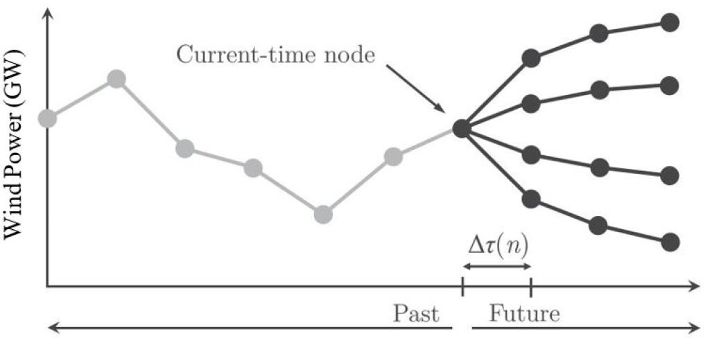
Figure 1: Schematic of a typical scenario tree used in SUC [8].

II-A Frequency Security Constraints

In [1], Teng et al show that inertia-dependent frequency security constraints can be derived from the swing equation. When these constraints are linearised and applied to the scheduling problem, frequency security following the loss of the largest power infeed is guaranteed at all times. This work was built on in [9] to incorporate FR with different delivery times, optimally allocated by a mixed integer second order cone program. Each FR service is modelled as a linear ramp with a magnitude $R$ GW delivered after a time $T$ s. FR must be delivered for 2 minutes, after which response from slower units, not modelled here, is assumed to bring the frequency back to its nominal value. A simplified version of these constraints that neglect system damping are presented here.

II-A1 RoCoF

The largest Rate of Change of Frequency (RoCoF) occurs at the instant of power infeed loss when no FR has been delivered. It is only limited by system inertia:

$$|RoCoF|=\frac{P_{l}\cdotp f_{0}}{2H(n)}\leq RoCoF_{max}$$ (2)

II-A2 Steady State

For the frequency to stabilise after a loss of generation, the amount of FR available must be at least equal to the power outage:

$$R_{E}(n)+R_{P}(n)\geq P_{l}$$ (3)

II-A3 Nadir

The frequency Nadir depends on both the available FR and the system inertia:

$$\bigg{(}\underbrace{\frac{H(n)}{f_{0}}-\frac{R_{E}(n)\cdotp T_{E}}{4\cdotp\Delta f_{max}}}_{=\ x_{1}}\bigg{)}\cdotp\underbrace{R_{P}(n)}_{=\ x_{2}}\geq\frac{(P_{l}-R_{E}(n))^{2}\cdotp T_{P}}{4\cdotp\Delta f_{max}}$$ (4)

Reference [9] notes that the nonlinear constraint (4) is in fact a rotated Second Order Cone that is convex because $x_{1}$ and $x_{2}$ are non-negative.

II-B Modelling of Aggregated EVs

In our model the aggregated EVs act as one large battery that is disconnected during the workday while the vehicles are in use. The aggregated battery’s state of charge (SOC) and power rates are equal to the sum of those for individual EVs. The normalised SOC of an individual EV is therefore the same as the normalised SOC of the aggregate battery. The highly predictable use profile of fleet EVs is fully specified by four parameters: the start/end time of a workday and the SOC at both of these times.

When formulating the optimisation problem the program iterates through the nodes sequentially from 1 to $N$, implementing constraints for each node’s specific set of decision variables. The absolute time $T_{ab}(n)$ of node $n$ is known during this phase.

If $T_{ab}(n)$ lies between $T_{out}$ and $T_{in}$ on a weekday, then no charging or discharging is allowed:

$$P_{d}\leq 0,\ \ \ P_{c}\leq 0\vspace{-0.1cm}$$ (5)

This effectively isolates the battery from the system, preventing any TSO service provision.

In the time interval when the vehicles leave the depot, i.e., when $T_{ab}(n)=T_{out}$, the SOC needs to meet the pre-specified energy requirement for driving:

$$E(n)=C_{out}\vspace{-0.1cm}$$ (6)

During time intervals when EVs are being driven, the energy demand for driving reduces the SOC to $C_{in}$ with no injection into the electricity system. The discharge rate $P_{d}$ of EVs following smart and unmanaged charging is always zero. Additionally, the FR capacity of unmanaged chargers is always constrained to zero and $T_{out}$ is set at a time occurring soon after $T_{in}$, forcing the EVs to charge immediately.

II-C Battery Degradation

Battery degradation in EVs manifests itself in two ways: capacity fade ($Q_{L}$), that reduces the maximum SOC; and power fade, which is associated with an increase in the internal resistance (IR) that reduces battery efficiency and limits the system’s power capabilities [10]. The user experiences an implicit cost of battery degradation through reduced EV performance and the need for more frequent EV replacement. Incorporating a degradation cost into the model allows the net system value of EVs to be calculated more accurately. In addition, explicitly considering the cost of degradation incentivises charging and discharging behaviour with a lower impact on battery life.

Battery degradation phenomena are dependent on multiple interacting factors that make model formation highly complex [11]. Nevertheless, battery ageing can be broadly divided into two components: calendar and cycle ageing. Respectively, the main factors to affect the two types of ageing are: SOC, calendar age and temperature; number of Full Equivalent Cycles (FECs), depth of discharge, charge rate and temperature.

This paper only considers a 10 kW charger attached to 40 kWh EV battery. Current mass-produced EV battery cells show cycle stability up to 6,000 FECs before a 20% capacity loss occurs [12] [13]. The maximum annual FEC number for any charging regime considered here is 263. Total ageing is a combination of cycle and calendar ageing. Consequently, over the minimum time of approximately 23 years required for the EVs simulated here to reach their maximum cycle number, the contribution of calendar ageing is dominant. For this reason cycle ageing is not considered in the SUC.

From extensive testing of lithium-ion batteries similar to those found in EVs, reference [5] proposes a calendar ageing model where $Q_{L}$ and IR only depend on temperature, SOC and age. Here, the temperature and age of individual EVs in the aggregate are unknown and uncontrollable so both of those terms are disregarded. The expression for IR as a function of SOC reported in [5] is concave. This too is disregarded due to the added complexity incurred when finding the system’s global optimum, but also because capacity fade is by far the more prevalent metric of EV degradation. The relationship between the capacity fade and the battery SOC is given by the following polynomial expression:

$$Q_{L}(n)=a_{1}(E(n)-0.5)^{3}+a_{2}\vspace{-0.1cm}$$ (7)

The coefficients ($a_{1}$, $a_{2}$) depend on EV battery age, temperature and type. Exact values of these coefficients are not known for a fleet of EVs so the values chosen here give a reasonable range of degradation rates based on the empirical data reported in [5]. It is important to emphasise that the objective of the paper is not to propose a highly accurate model for EV battery degradation cost. Rather, it is to see how operation might vary when the cost of EV battery degradation is explicitly considered and how this might impact the value of EVs to the system.

In this paper $a_{1}=5.70\times 10^{-4}$ and $a_{2}=5.70\times 10^{-5}$ are used. This gives absolute annual degradation rates similar to those presented in Fig. 2a of [5] for a battery held at SOC = 0.5 and $0^{o}$C. Furthermore, these coefficients give a ratio of $min(Q_{L}):max(Q_{L})=0.45$ which is within the range presented in Fig. 7a of [5]. Fig. 2 shows the capacity fade for an individual EV stored at a constant SOC for a year using these coefficients.

$Q_{L}$ is non-convex so it is approximated by two linear inequality constraints before being added to the SUC:

$$Q_{L}(n)\geq\alpha_{1}E(n)+\alpha_{2}$$ (8)

$$Q_{L}(n)\geq\beta_{1}E(n)+\beta_{2}$$ (9)

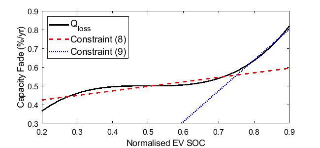
Figure 2: Cubic relation between capacity fade and SOC, shown with the linear approximation when $\omega=0.76$.

The coefficients used in this paper are $\alpha_{1}=2.76\times~{}10^{-5}$, $\alpha_{2}=4.29\times 10^{-5}$ and $\beta_{1}=1.88\times 10^{-4}$, $\beta_{2}=-7.76\times 10^{-5}$. These are found via linear regression between the boundary SOCs (0.2 and 0.9) and a shoulder value $\omega$. Here $\omega=0.76$ is chosen because the capacity fade at this SOC is halfway between the capacity fade value at the boundary SOCs. Finally, because $Q_{L}$ gives the relative capacity fade of an individual EV it is multiplied by the number of EVs and a cost coefficient $c^{D}$ in the modified objective function:

$$\sum_{n\epsilon N}\pi(n)\bigg{(}\sum_{g\epsilon G}C_{g}(n)+\delta\tau(n)(c^{LS}P^{LS}(n)\\ +c^{D}Q_{L}(n)N_{EV})\bigg{)}$$ (10)

III Case Studies

To explore the cost reductions offered by different grid-connected EV configurations, the SUC model described in section II was used to run a number of case studies simulating the annual operation of a representative GB 2025 system. A wide range of assumptions has been studied for the number of fleet EV connected to the system, ranging between 50,000 and 300,000. For each fleet EV penetration and each of the three charging regimes the value of EV was found as the difference in annual operating cost between a given fleet EV case and the benchmark case with zero EVs, and then divided with the assumed number of EVs.

The system was assumed to include 55 GW of thermal generation capacity, with the characteristics taken from Table I of [8]. The fleet includes 4 must-run 1.8 GW nuclear plants, thus $P_{l}$ = 1.8 GW. Two types of FR are considered: EFR with delivery time $T_{E}=1~{}s$; and PFR with delivery within $T_{P}=10~{}s$. Batteries (including aggregated EVs) are assumed to provide EFR, while thermal and pumped storage plants provide PFR. In line with GB grid standards the frequency criteria of $RoCoF_{max}=$ 1 Hzs^-1 and $\Delta f_{max}=$ 0.8 Hz were assumed. A scenario tree that branches at the current node only (refer to [7] for further explanation) was used for the SUC with quantiles of 0.005, 0.1, 0.3, 0.5, 0.7, 0.9 and 0.995 considered. Historic electricity demand data profile is used in the model, ranging from 25 GW to 60 GW. Unless otherwise specified there is 30 GW of installed wind capacity and 1 GWh/0.25 GW stationary battery storage on the system. There is also 10 GWh/2.6 GW pumped hydro storage capacity on the system capable of providing 0.5 GW of PFR.

Each EV in the fleet is assumed to have a battery with 40 kWh capacity with a normalised SOC range limited between 0.2-0.9, (dis)charge efficiency of 96% and maximum (dis)charge of 10 kW. The vehicles are disconnected from the grid between 08:00 and 16:00 during working days, with $C_{out}$ = 0.9 and $C_{in}$ = 0.625. $T_{out}$ for unmanaged chargers was set to 21:00. No EVs other than the fleet vehicles were connected to the system. Only section III-C considers battery degradation.

III-A Value of EV for various charging regimes

The system values of EVs obtained across various EV uptake levels and charging regimes are shown in Fig. 3. The results clearly show that V2G is more valuable to the system than Smart for all EV penetrations. With 50,000 EVs on the system each V2G-enabled fleet EV can reduce the system operation cost by £12,000 per annum and CO₂ emissions by 60 tonnes per annum whilst meeting all driving requirements. As expected, unmanaged charging increases system costs (i.e., results in a negative value per EV) because it increases the system energy demand without offering any TSO services.

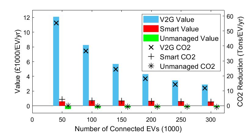
Figure 3: Annual system cost savings and CO₂ emission reduction per EV for various charging regimes and EV penetrations.

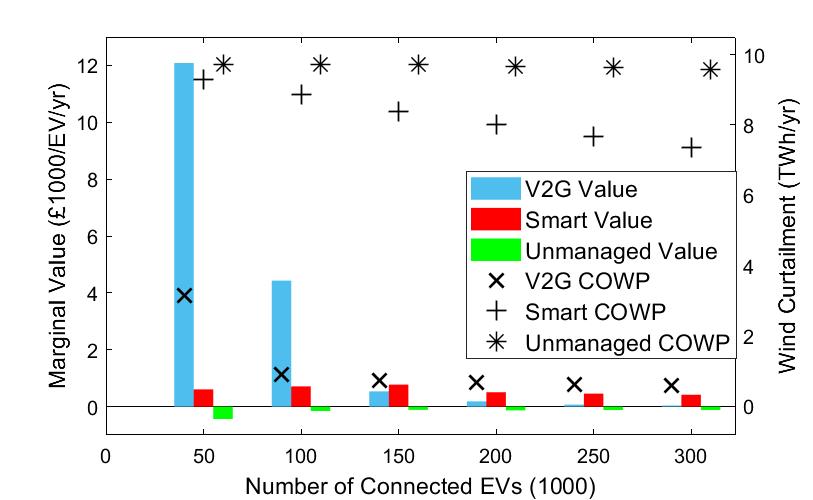
Figure 4: Marginal system value per EV at various EV penetrations plotted with total annual wind curtailment.

Reduced COWP is the main contributor to the observed cost and emission reductions. This is demonstrated in Fig. 4, which quantifies the marginal system value per EV, obtained by finding the cost difference between two adjacent EV penetrations and dividing it with the difference in EV numbers for the two penetrations. The marginal value of V2G-enabled EVs appears to be broadly proportional to the trend of reducing COWP. 50,000 EVs with V2G enable the system to absorb 6.1 TWh more wind energy than with smart charging, or about 6.7% of the annual available wind output.

Frequency security constraints effectively impose a limit on the minimum level of system inertia. In the model presented in this paper inertia is only provided by thermal plants; however, FR can be provided by both thermal plants and storage. Thermal plants have MSG limits so a minimum system inertia can also be expressed as a requirement for Minimum System Thermal Generation (MSTG). COWP occurs when the sum of MSTG and the available wind power becomes higher than system demand.

Fig. 5 plots the the relationship between MSTG and available FR capability resulting from constraints (2) and (4), if there was only one FR service with a delivery time of 1 s or 10 s. The MSTG driven by the RoCoF is independent of FR. Therefore, when sufficient FR is available from EVs to reduce the nadir-driven MSTG below that required to ensure maximum RoCoF, the value of additional EVs reduces significantly because the incremental FR they can provide does not reduce the system’s MSTG.

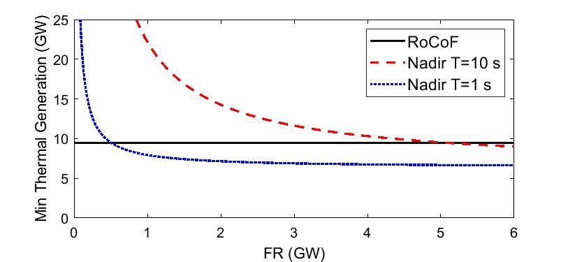
Figure 5: Minimum thermal generation to provide inertia to secure system frequency for a given level of FR. The nadir inertia requirement is derived from (4) with one FR service (i.e. $R_{E}=0$) with two different delivery times.

V2G-connected EVs can provide EFR at all times other than when discharging at maximum rate, while EVs in the Smart charging regime can only provide FR whilst charging, as shown in Fig. 6. This means that the saturation point in EFR value is reached with far fewer V2G, explaining their higher average value and quickly saturated marginal value. This agrees with the work in [14] that suggests that at low EV penetrations V2G services are extremely valuable, but at high EV penetrations system FR requirements can largely be met through smart charging.

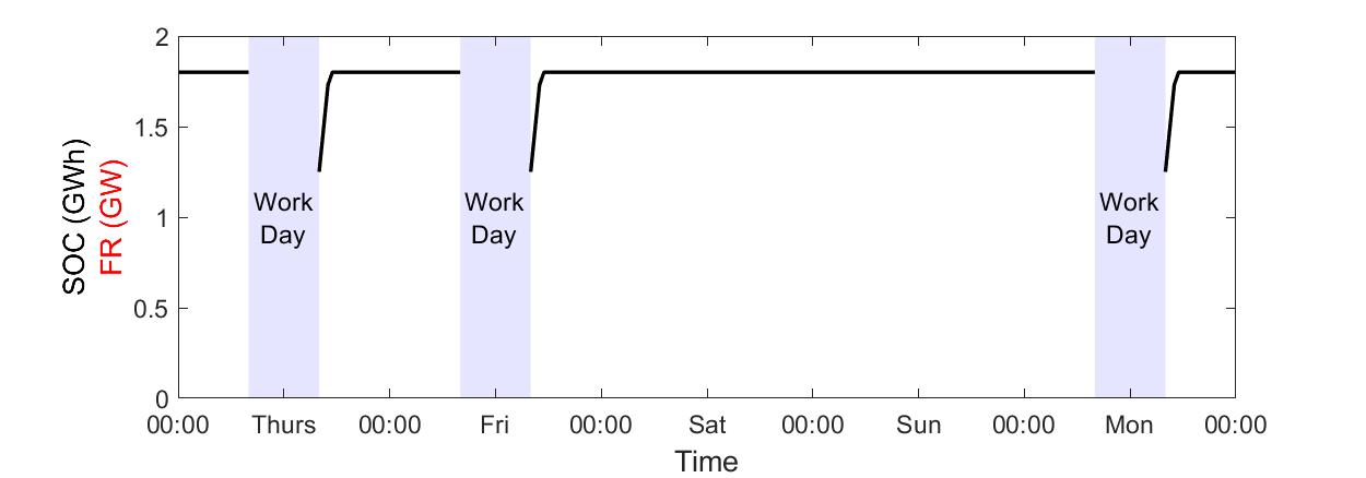
(a)

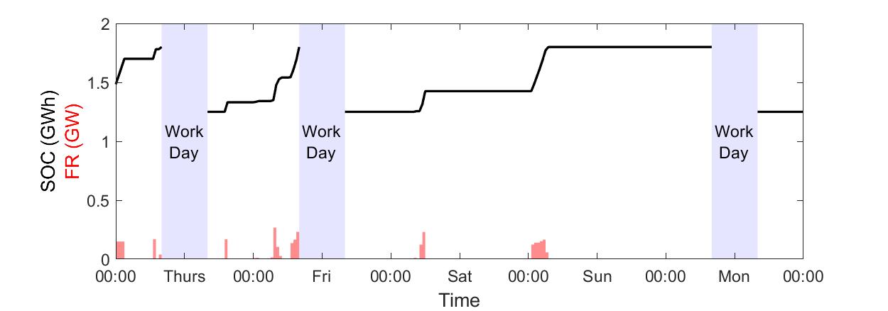
(b)

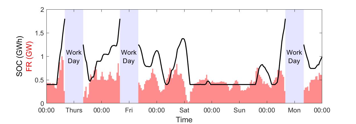
(c)

Figure 6: SOC and FR provision from EVs over a typical 5-day period for a 50,000 EV fleet with three different charging capabilities: (a) Unmanaged, (b) Smart and (c) V2G.

COWP can also be reduced by charging EVs to increase the system demand during high wind periods, but this is a secondary effect. Although reduced COWP is the dominant value driver, the EVs also create value from: providing reserve thus reducing the need for expensive OCGT plants; increased efficiency of higher loaded online thermal plants and fewer turn on/off events.

III-B Impact of wind generation and competing flexibility providers on the value of EVs

System value of EVs is heavily dependent on the characteristics of the system they are added to. This section presents the sensitivity of the EVs’ value to renewable penetration, competing flexibility and FR delivery time. The number of EVs in all studies presented in this section was fixed at 50,000. For conciseness only Smart and V2G results are analysed below.

Table. I shows the change in the EV value as wind capacity increases from 30 GW to 45 GW and 60 GW, as well as the changes in COWP. The value of V2G increases approximately in proportion to the increase in installed wind capacity. The value of Smart remains largely constant over the wind penetrations considered. In line with the discussion in section III-A, reduced COWP is the main value driver. Higher wind capacity increases the amount of time and the magnitude by which the sum of the wind power and the MSTG required for frequency security exceeds demand. This occurs frequently enough with 30 GW of wind capacity that the limited EFR capability of smart chargers is already fully utilised to reduce curtailment, so no additional value is gained. On the other hand, because V2G can provide EFR when idle, MSTG is reduced significantly for most non-workday hours. This means that the instances of COWP are less frequent and of a lower magnitude.

TABLE I: Dependence of EV Value on the Penetration of Wind Generation

	Value (£/EV/yr)		Wind Curtailment
			(TWh/yr)
Wind Capacity	Smart	V2G	Smart	V2G
30 GW	608	12,088	9.28	3.16
45 GW	590	19,769	34.92	22.19
60 GW	611	23,812	69.26	53.07

TABLE II: Dependence of EV Value on the Penetration of Battery Storage

	Value (£/EV/yr)
Battery Capacity (GW:GWh)	Smart	V2G
0.25:1	608	12,088
0.5:2	203	9,070
1.0:4	47	1,921
1.5:6	-128	475
2.0:8	-125	335

If EVs are exposed to competition from other flexible sources such as other forms of battery storage, their value can reduce significantly. This is true whether that storage is from other EVs, as in Fig. 3, or from standalone grid-connected batteries, as shown in Table II. This is because when EFR is plentiful, the nadir constraint can be secured easily. After this the MSTG is limited by the thermal plants whose inertia is needed to secure the system RoCoF, upon which additional storage has little effect. It is interesting to note that in Table II, for 1.5 GW and 2 GW of battery storage, the marginal value of EFR is reduced to the point that the cost of the increased energy demand from a smart charger is not offset by its FR provision, resulting in negative system value i.e., positive net system cost per EV.

Finally, the sensitivity on FR delivery times presented in Fig. 7 demonstrates that FR provision represents the majority of the system value of V2G-connected EVs. Value per EV is reduced by 95% from £12,088 to £643 when it provides no FR. This is attributable to the 6.3 TWh increase in annual COWP that occurs when the MSTG is not reduced by the EVs. The speed of FR delivery is also an important value driver: increasing the delivery time from 1 s to 10 s reduces the value of V2G-enabled EVs by about two thirds.

III-C Battery Degradation

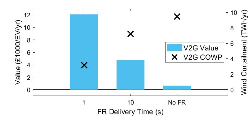
Figure 7: System value of a V2G connected EV with different FR speeds.

This section applies the battery degradation model developed in section II-C to a system with 300,000 EVs. A $c^{D}$ of £1,500/% was used, implying that a £30,000 EV must be replaced after a 20% capacity fade. To calculate degradation during the workday driving cycles, the SOC is assumed to be at $C_{out}$ and $C_{in}$ for 4 hours each.

Fig. 8 shows how V2G-connected EV operation varies over the same 5-day period when degradation is penalised in the cost function. For the case where degradation is penalised, corresponding to the cost function (10), the EVs’ SOC is mostly maintained below 0.75 (9 GWh), as this region corresponds to constraint (8), and therefore results in lower degradation costs.

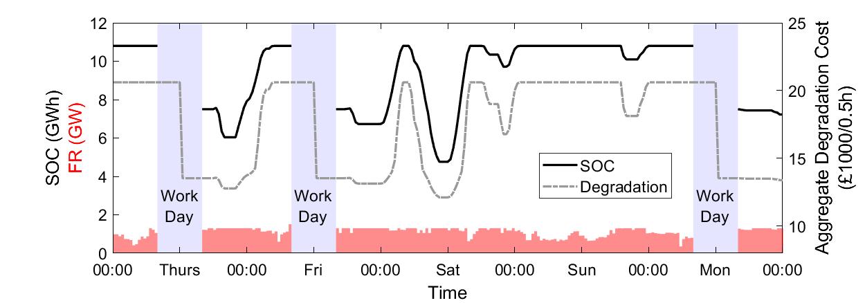
(a)

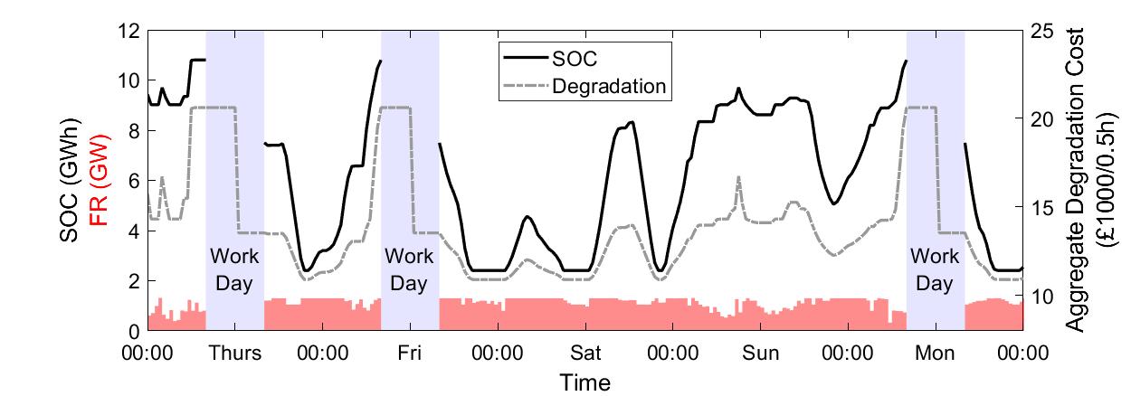
(b)

Figure 8: FR allocation and SOC over a typical 5-day period for 300,000 V2G connected EVs. When the SOC is greater than $\omega$, $Q_{L}$ lies on (9). (a) Degradation is not penalised, cost function (1) used. (b) Degradation is penalised, cost function (10) used.

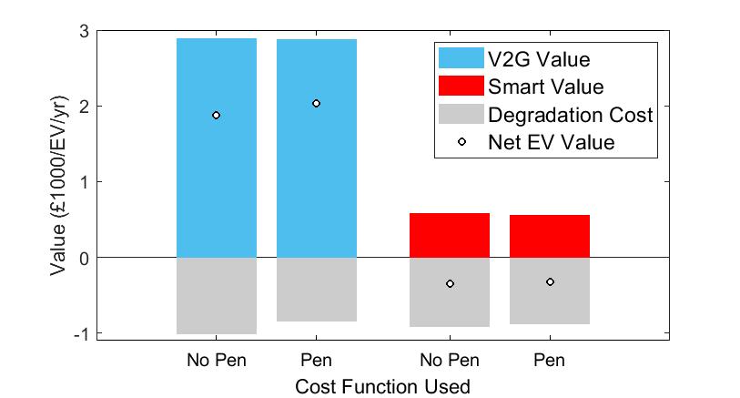
Figure 9: Net value of both smart and V2G connected EVs when degradation is (Pen) and is not (No Pen) penalised in the objective function.

As shown in Fig. 7, the majority of the system value of EVs derives from the EFR they provide to the system, reducing the COWP as a result. Fig. 8 demonstrates that EFR provision is largely independent of the SOC, so is similar regardless of whether cost function (1) or (10) is used. Therefore, incorporating a degradation model into the SUC enables a significant reduction in the EV battery degradation cost of 16.3%, for only a small decrease in its system value of 0.4%. This is illustrated in Fig. 9, which shows the net value of V2G and Smart EVs after factoring in the cost of battery degradation for two cases. The first (No Pen) minimises objective function (1) but subsequently adds the degradation cost based on the SOC variations. The second (Pen) is obtained by minimising (10) i.e. explicitly considering the degradation cost. It can be observed that the net value of a V2G-enabled EV increases by £154 if battery degradation is explicitly considered in cost minimisation.

IV Conclusion

This paper presented a frequency-constrained SUC model that considers aggregated fleet EVs while incorporating the vehicles’ driving constraints. The SUC model has been used to demonstrate the impact on system operation cost and carbon emissions when fleet EVs connect to the grid with different charging regimes. FR provision was identified as a key value driver for V2G and Smart charging approaches in a system with high penetration of wind generation, although the EV value was found to be highly sensitive to the uptake of competing flexible options such as standalone batteries and to the speed of FR delivery. A linearised battery degradation model was implemented in the scheduling problem and was used to demonstrate that large decreases in degradation are possible, with only minor reductions in the value of EVs.

Future work will incorporate uncertainty in the driving times and energy usage of EVs into the scheduling process. This will allow value comparison between EVs with different usage profiles, such as fleet or domestic. In addition, work focused on market structures that efficiently convert the demonstrated system cost reductions into revenues for the EV owner will be needed.

References

- [1] F. Teng, V. Trovato, and G. Strbac, “Stochastic Scheduling with Inertia-Dependent Fast Frequency Response Requirements,” IEEE Transactions on Power Systems, vol. 31, pp. 1557–1566, mar 2016.
- [2] A. Tuohy, P. Meibom, E. Denny, and M. O’Malley, “Unit commitment for systems with significant wind penetration,” IEEE Transactions on Power Systems, vol. 24, no. 2, pp. 592–601, 2009.
- [3] H. Lund and W. Kempton, “Integration of renewable energy into the transport and electricity sectors through V2G,” Energy Policy, vol. 36, pp. 3578–3587, sep 2008.
- [4] “Vehicle to Grid Britain,” tech. rep., Element Energy Limited, 2019.
- [5] M. Naumann, M. Schimpe, P. Keil, H. C. Hesse, and A. Jossen, “Analysis and modeling of calendar aging of a commercial LiFePO4/graphite cell,” Journal of Energy Storage, vol. 17, pp. 153–169, jun 2018.
- [6] “PLUGGED-IN FLEETS A guide to deploying electric vehicles in fleets,” tech. rep., The Climate Group, Cenex, Energy Saving Trust, 2012.
- [7] A. Sturt and G. Strbac, “Efficient stochastic scheduling for simulation of wind-integrated power systems,” IEEE Transactions on Power Systems, vol. 27, pp. 323–334, feb 2012.
- [8] L. Badesa, F. Teng, and G. Strbac, “Simultaneous Scheduling of Multiple Frequency Services in Stochastic Unit Commitment,” IEEE Transactions on Power Systems, pp. 1–1, mar 2019.
- [9] L. Badesa, F. Teng, and G. Strbac, “Optimal portfolio of distinct frequency-response services in low-inertia systems.” (in review). Preprint available at: https://arxiv.org/pdf/1908.07856.pdf, 2019.
- [10] A. Barré, B. Deguilhem, S. Grolleau, M. Gérard, F. Suard, and D. Riu, “A review on lithium-ion battery ageing mechanisms and estimations for automotive applications,” Journal of Power Sources, vol. 241, pp. 680–689, 2013.
- [11] J. Vetter, P. Novák, M. R. Wagner, C. Veit, K. C. Möller, J. O. Besenhard, M. Winter, M. Wohlfahrt-Mehrens, C. Vogler, and A. Hammouche, “Ageing mechanisms in lithium-ion batteries,” Journal of Power Sources, vol. 147, pp. 269–281, sep 2005.
- [12] “Kokam battery cells, lithium ion polymer cells - high energy high power.” http://kokam.com/cell/. Accessed: 2020-03-10.
- [13] M. Yasuda, “Sony energy storage system using olivine type battery,” International Conference on Olivines for Rechargeable Batteries, Montreal, 2014.
- [14] F. Teng and G. Strbac, “Full Stochastic Scheduling for Low-Carbon Electricity Systems,” IEEE Transactions on Automation Science and Engineering, vol. 14, pp. 461–470, apr 2017.