Implementation of a generalized precession parameter in the RIFT parameter estimation algorithm
I. Introduction
In the modern era of gravitational wave astronomy, data obtained by the Advanced LIGO and Advanced Virgo detectors offers fresh insights on the characteristics of coalescing binary black holes (BBHs) [1, 2, 3, 4]. Analysis of these data has afforded us a new window on the dynamics of such astrophysical systems, and we are now able to identify the detailed characteristics of their evolution.
To date a total of 90 gravitational wave events have been observed [4], and it is predicted that in O4 the LIGO-Virgo-KAGRA (LVK) network will detect binary neutron star (BNS) mergers, neutron star-black hole (NSBH) mergers, and BBH mergers [5, 6]. By comparing the recorded signal to that produced by simulated waveforms, we can obtain statistical information about the fundamental source parameters of the binary system. The collaboration currently uses a number of parameter estimation programs, including LALInference [7], Bilby [8], and RIFT [9, 10]. These codes construct posterior probability distributions for the binary’s intrinsic parameters which may then be procedurally transformed into other characteristic parameters to assess the properties of a binary. Such parameterizations are useful both as a comparative heuristic for analysis, and also as a sampling coordinate for improved parameter estimation. One of the properties of a binary system that can be effectively reduced to a parameter is its precession - the change in direction of the binary’s orbital angular momentum over time.
The characteristics of a gravitational waveform will be distinctly altered if the source binary contains objects with misaligned spins - i.e. the spin angular momenta of the individual objects do not point in the same direction as the orbital angular momentum of the binary. In such systems the orbital plane will precess about the direction of the total angular momentum [11]. Spin-precession affects the gravitational waveform in three ways (1) it contributes to the orbital decay of the binary, and thus to the accumulated phase of the gravitational wave; (2) it causes the orbital plane to precess, changing its orientation relative to us and thus modulating the waveform; and finally (3) spin contributes directly to the gravitational wave amplitude through higher order terms in the post-Newtonian expansion[12].
The identification and analysis of precessing systems can have a significant impact in our understanding of astrophysical binary formation channels. There are two primary ways that these binaries can form. The first is in the heart of star clusters [13, 14, 15]: in these dense environments dynamic interactions between systems can lead to spins becoming misaligned; e.g. in young star clusters [16]. The second primary formation channel occurs in isolated systems in the galactic field [17, 18, 19], where there are several possible mechanisms of formation. Of particular interest are binaries formed through supernova kicks, where it is estimated that as high as 80% of objects can have misalignment angles greater than 30°[20].
In order to rapidly identify spin-precession effects in gravitational wave signals, the raw output of parameter estimators such as RIFT is recast into single effective parameters such as (see Eq.(2) that judge the degree to which a binary is precessing. is a parameter that expresses the maximum misaligned spin in the binary, taking information from only one of the two objects. In this work we shall discuss the implementation in RIFT of the updated precession parameter , first introduced in [21]. This new parameter is a more faithful characterization of a binary’s precession, as it includes misalignment information from both objects in the binary and averages over all the angular variations on the precession timescale. It will be shown that there are significant differences in the valuation of precession between these two parameters, particularly for systems with large spin magnitudes and even mass ratio . The expression of these differences will then be highlighted for select events from O3b, of which ten show large amounts of precession .
This work will be organized as follows. In Sec.(II) we review the parameterization of precession magnitude as a way to characterize the binary. Following [21], in Sec.(III) we describe the implementation of in the RIFT parameter estimation algorithm. In Sec.(IV) the differences between the current standard parameter and the updated parameter are discussed as functions of the intrinsic parameter space. Finally in Sec.(V) the precession characteristics for all 36 events from the second half of the Advanced LIGO and Advanced Virgo third operating run (O3b) are reported and discussed.
II. Parameterizing Precession
In a binary system containing objects with arbitrarily oriented spins, the spin-precession behavior may be entirely defined by eight intrinsic parameters: the two object masses and six spin components . To analyze such systems we take the coordinate system as shown in Fig.(1), following [22]. We also take the convention for the mass ratio .
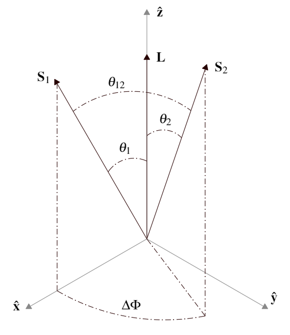
In a coalescing binary the evolution of the orbital angular momentum per orbit proceeds as follows:
| (1) |
where the first term describes the orbital plane precession - the change in the direction of the orbital angular momentum over time, and the second term describes the radiation reaction. These two effects happen on different timescales and can thus be decoupled from each other. The first scalar parameter introduced to characterize precession, presented in [23], defines as:
| (2) |
where is the ratio of spin frequencies to leading order:
| (3) |
As defined in Eq.(2), is the precession parameter has previously been widely reported by standard parameter estimation codes to assess the degree to which a binary is precessing. The normalization factor of constrains this parameter to the region , with a larger value indicating a larger degree of spin misalignment and thus orbital plane precession. This parameter is derived from the normalized magnitude of orbital plane precession, which we refer to as the generalized :
| (4) |
by taking the average value of the extrema. However as pointed out by Gerosa et al. [21] this parameter has several drawbacks. Consider that as defined in Eq.(2) effectively judges only the larger of the two spin projections onto the orbital plane; i.e. it takes information from only one of the two objects in the binary. Furthermore the reductive assumption of taking only the extrema of is tantamount to averaging over only this angle; however the other two relevant angles vary on the same timescale. As all three angles vary on the same timescale , information is lost by averaging over only one of the three. A resolution to this problem involves averaging over all the angular variations on the precession timescale. This new parameterization takes the general definition of Eq.(4) and computes the average:
| (5) |
where is chosen as a quantity that characterizes the one-parameter spin precession dynamics on the spin precession timescale. The averaged precession parameter retains information from both objects in the binary, and is a constant of motion at 2PN. It is also constrained to the domain , with the region exclusive to binaries with two misaligned spins. For the implementation in RIFT presented below, the total spin magnitude was chosen for , as it is easily obtained from the intrinsic parameters without need for further transformation.
III. Implementation
i. RIFT
Rapid Iterative FiTting (RIFT) [9, 10] is a parameter estimation algorithm that compares a candidate coalescing binary gravitational wave signal to existing waveforms, then marginalizes the likelihood of the signal data over the characteristic coordinates of the binary’s coalescence event relative to the Earth. The basic procedure for using RIFT222For more information on using RIFT and associated functions, see https://github.com/oshaughn/RIFT_tutorials.is simple. Metadata from a gravitational wave candidate event is taken directly from GraceDB (the Gravitational-Wave Candidate Event Database). The user then chooses an approximant; the type of simulation basis template against which the real data will be compared. RIFT also allows for several options, such as specifying the power spectral density (PSD), allowing for higher-order modes, number of iterations, etc.
From this user input, RIFT goes through two primary stages. The first is Integrate Likelihood Extrinsic (ILE), which evaluates the marginalized likelihood on candidate points using Monte Carlo integration. The second stage is Construct Intrinsic Posterior (CIP), which then estimates the likelihood and posterior distribution using a Gaussian process. This posterior is then used as a prior in the next iteration, and the two tasks repeat. The output of RIFT is a set of posterior probability distributions for the binary’s eight intrinsic parameters and if specified, also the extrinsic parameters. For any specific sample within this distribution, one may then conduct any transformation dependent upon these parameters. For a trivial example one might compute the mass ratio , and do so for every sample to create a posterior distribution.
The RIFT package provides many standard parameter transformations (lalsimutils.py), as well as a plotting tool (plot_posterior_corner.py) for creating corner plots of the posterior distributions. We modified these two utilities to calculate and illustrate the averaged precession parameter . We emphasize these calculations are purely postprocessing, performed after the main parameter estimation process of RIFT. As they require only posterior samples, such calculations can be subsequently performed with any existing posterior data. These low-cost postprocessing transformations can be performed readily with local CPUs.
ii. Calculation of in RIFT
To calculate for a given set of eight intrinsic parameters, the following algorithm has been programmed into RIFT’s lalsimutils.py analysis tool as an option in the extract_param function. This closely follows the example implementation presented in [21] (and implemented with the precession package [24]), with adjustments made to cooperate with RIFT’s existing functions. It should be noted that the RIFT output samples for the two masses are given in the units of solar mass ; for the purposes of this calculation we therefore first convert these to units of using the conversion factor to reduce the numerical order across the rest of the algorithm. We begin by calculating the angles using the built-in function extract_system_frame. This function first fixes the direction of orbital angular momentum (see Fig.(1)) and then computes the following:
| (6) |
The function extract_system_frame also gives us the dimensionless spin magnitudes . The mass ratio is defined as with . The last value needed is the reference frequency , which is given a default value of , although this may be changed through user specification. The (Newtonian) orbital angular velocity is then . We can now calculate the separation distance as per Eq.(4.13) in Ref. [12]:
| (7) |
We then proceed to calculate the magnitude of the angular momentum , the magnitude of the total angular momentum , and the dimensionless effective aligned spin [25, 26]:
| (8) |
| (9) |
| (10) |
Note that is a conserved quantity on both the precession and radiation-reaction timescales [24]. Recall that our goal is to calculate Eq.(5) using the total spin; this equation now becomes:
| (11) |
The time derivative of is given by [25]:
| (12) |
Notice that this derivative contains angular parametric equations of , which are given by:
| (13) |
The limits of integration in Eq.(15) correspond to the two extremal solutions of . To obtain these we use the function Sb_limits, which is part of the precession package [24]. This evaluates the geometrical constraints of the system based on the following definitions. As shown in Fig.(1), the two polar angles range from and the azimuthal angle difference ranges from . Based on the limits of the polar angles and azimuthal angle difference, the effective spin , along with the total spin , and the total angular momentum , also have geometric limits:
| (14) |
Notice that these constraints are dependent on each other. To solve for the limits , the effective potentials [27] for spin precession are used:
| (15) |
The solutions to the equations are then found using scipy.optimize.brentq, an implementation of Brent’s method for root finding. Each of the integrals in Eq.(15) may now be calculated, and are computed by scipy.integrate.quad. Note that the precession cycle is symmetric; as such we need only integrate over half of the total cycle (i.e. from to ).
Given the input of the eight intrinsic binary parameters this algorithm computes a value for which lies in the interval . However it should be noted that this procedure does fail for a few specific cases. If both spins are entirely aligned (or anti-aligned) with the orbital angular momentum, then the above algorithm will fail. However this is a trivial case, as if there is no misalignment then there is no precession and we set . If one of the spins is exactly zero (i.e. ) but the other spin is not, then this algorithm also fails. In this case , and this is the parameter that is calculated. This equivalence can be seen by applying the single misaligned spin condition to Eq.(4) for the generalized precession parameter. Here taking :
| (16) |
Or the opposite case, where :
| (17) |
Hence a comparison to Eq.(2) shows that for either case of single misaligned spin calculation of the general precession parameter reduces to simply a calculation of . This is true also for the averaged precession parameter ; as the magnitude of one of the spins approaches zero, is well approximated by .
RIFT’s supplemental tool for plotting posterior probability distributions is plot_posterior_corner.py, which reads in the posterior samples produces by the ILE/CIP process and creates corner plots of the total probability distribution for the binary. Within this script one can call any of the transformations programmed into lalsimutils.py to similarly create posteriors for parameters such as . This parameter has been included in the latest release of RIFT, and posteriors for both precession parameters can now be created for any existing and future gravitational wave event data.
IV. Parameter Comparison
Let us now examine the key differences between these two precession parameters. The current standard parameter looks at the projection of the two object’s spins onto the orbital plane, and takes the maximum of these two values. This produces a parameter value normalized to the domain . However by taking this maximum we are considering information from only one of the objects in the binary, and using this information alone to judge spin misalignment and thus orbital plane precession. This method, while useful in specific cases, loses the cross term from the generalized precession parameterization given in Eq.(4).
The new parameter retains this term and averages over on the precession timescale, and as such retains the spin-misalignment information from both objects in the binary. This produces a parameter value normalized to the domain . As pointed out in [21], it is of crucial interest to note that any value of must necessarily correspond to a set of binary intrinsics where both objects have misaligned spin. This is an immediately observable feature that is not present in , as from this parameter there can be no direct correlation to the intrinsic space of both objects.
Based on the domains of these two parameters, at first glance one might expect that for a given set of source parameters will yield values greater than . However the inclusion of the cross term which contains in Eq.(4) means that for specific binary morphologies the averaged parameter can actually be much less than . To highlight this, a set of uniformly random binaries was generated with spin components . For each of these binaries both and were calculated at fixed total mass, for mass ratios at a reference frequency of . It should be noted that the spin component values were randomized with a fixed seed; the only variable changing between the three tests below is the mass ratio. The data from these calculations are shown in Fig.(2) below.
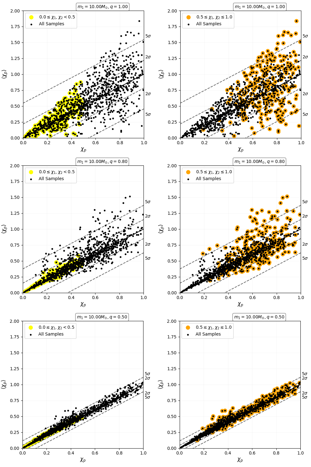
One can see that for binaries in which both objects have relatively high spin the distribution of the parameter space will be more widely spread about the line, in some cases surpassing a deviation. For binaries in which both objects have a relatively low spin the distribution of the parameter space will be less widely spread about the line, never exceeding . This difference relationship also depends strongly on the mass ratio , but not on the total mass. The mass ratio enters as a variable in the normalizing factor (Eq.(3)). One can see that increasing the asymmetry in reduces the overall spread of the parameter difference for all spin values. At higher inverted mass ratios the parameter difference is negligible, and in the limit as the two parameters converge. The parameter difference also depends strongly on the azimuthal angle difference . This variable enters into Eq.(4) as a cosine term, and this behavior is reflected in the distribution as shown in Fig.(3).

Notice that for the distribution of values tends to follow the behavior of , but as the mass ratio decreases the distribution appears more uniform. Consider first the image. The samples with the largest positive parameter difference cluster around the regions, corresponding to spin morphologies where the in-plane components of are aligned. These regions, where also represent the domain in which . These samples, highlighted in red, correspond to binaries that necessarily have two misaligned spins - qualitative information that is not conveyed by . The samples with the largest negative difference cluster in the region surrounding , where . This region corresponds to spin morphologies where the in-plane components of are anti-aligned. The orthogonal conditions for in-plane spin components correspond to roots in vs. , indicating that for these morphologies the two parameters are equivalent. However these behaviors degrade as the mass ratio decreases. Progressing from left to right in Fig.(3), the cosine-like behavior of vs. loses definition and approaches a uniform distribution. Additionally the quantity of samples with is significantly reduced, indicating that this region is less useful as a qualitative heuristic for double-misalignment as the mass ratio deviates from unity.
These results demonstrate that for practically any given spin morphology, the parameter either under or overestimates the binary’s precession. This is because inherently takes information from only one object in the binary, and does not take into account all the angular variations of the two objects over the precession timescale. However, is still a useful parameter when the mass asymmetry is large, or if one of the two spins is close to zero where as discussed in Sec.(ii).
V. Precession Results from GWTC-3
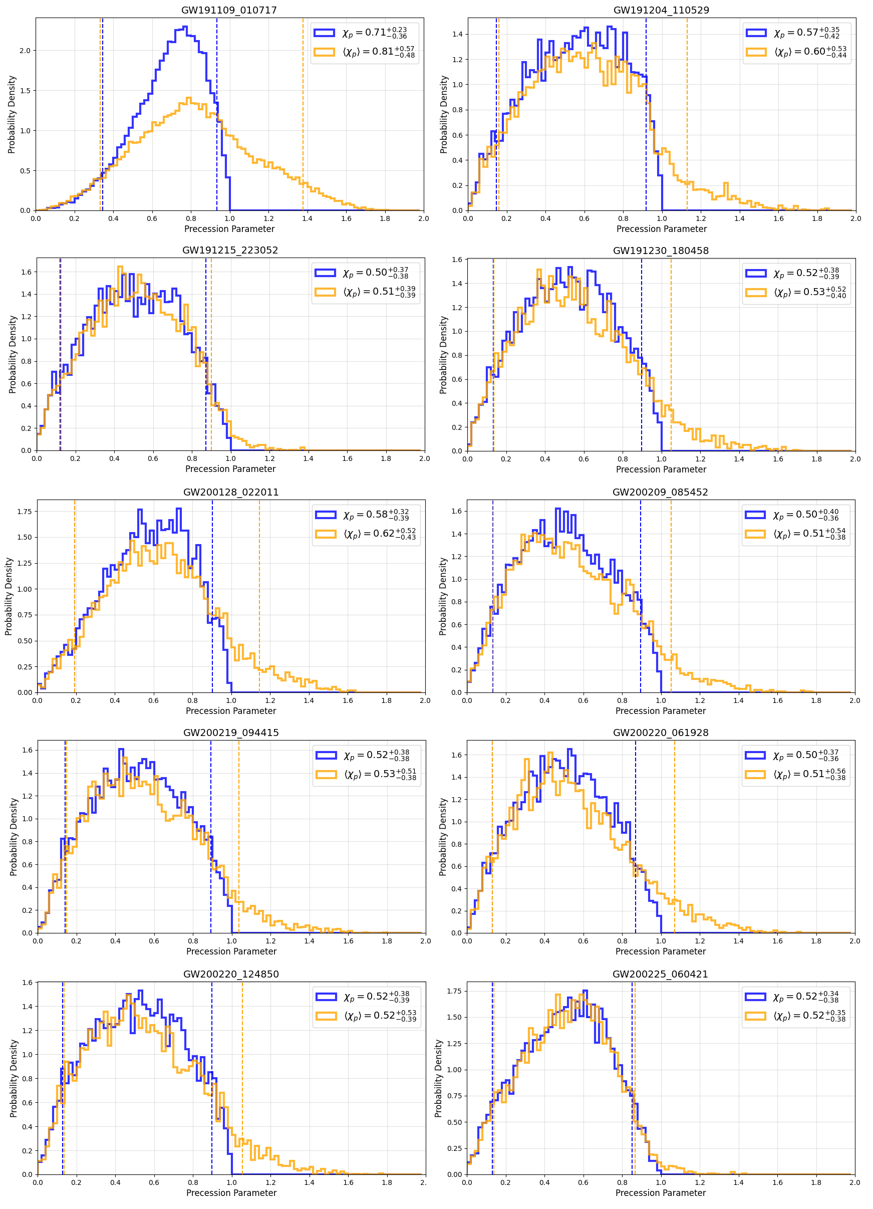
Presented below are the precession parameter posteriors for all 36 events from the second half of the Advanced LIGO and Advanced Virgo third observing run, as presented in GWTC-3 [4]. The intrinsic parameter data used to calculate these come from the public release [28, 29], and were converted to RIFT readable format using the PESummary python package [30]. From this release the SEOBNRv4PHM [31] approximant samples created by RIFT (prior to spin evolution and cosmological re-weighting) were analyzed. These data were chosen to be as close to the raw RIFT output as possible, differing only by standard calibration adjustment. As such the data shown here may differ from those reported in the O3b catalog, which use a combination of samples from both the time-domain parameter estimation (RIFT, SEOBNRv4PHM) and frequency-domain parameter estimation (Bilby, IMRPhenomXPHM [32]). Presented here are posterior probability distributions for both and , displayed in Fig.(4) below, with median and 90% confidence intervals reported in Table(2).
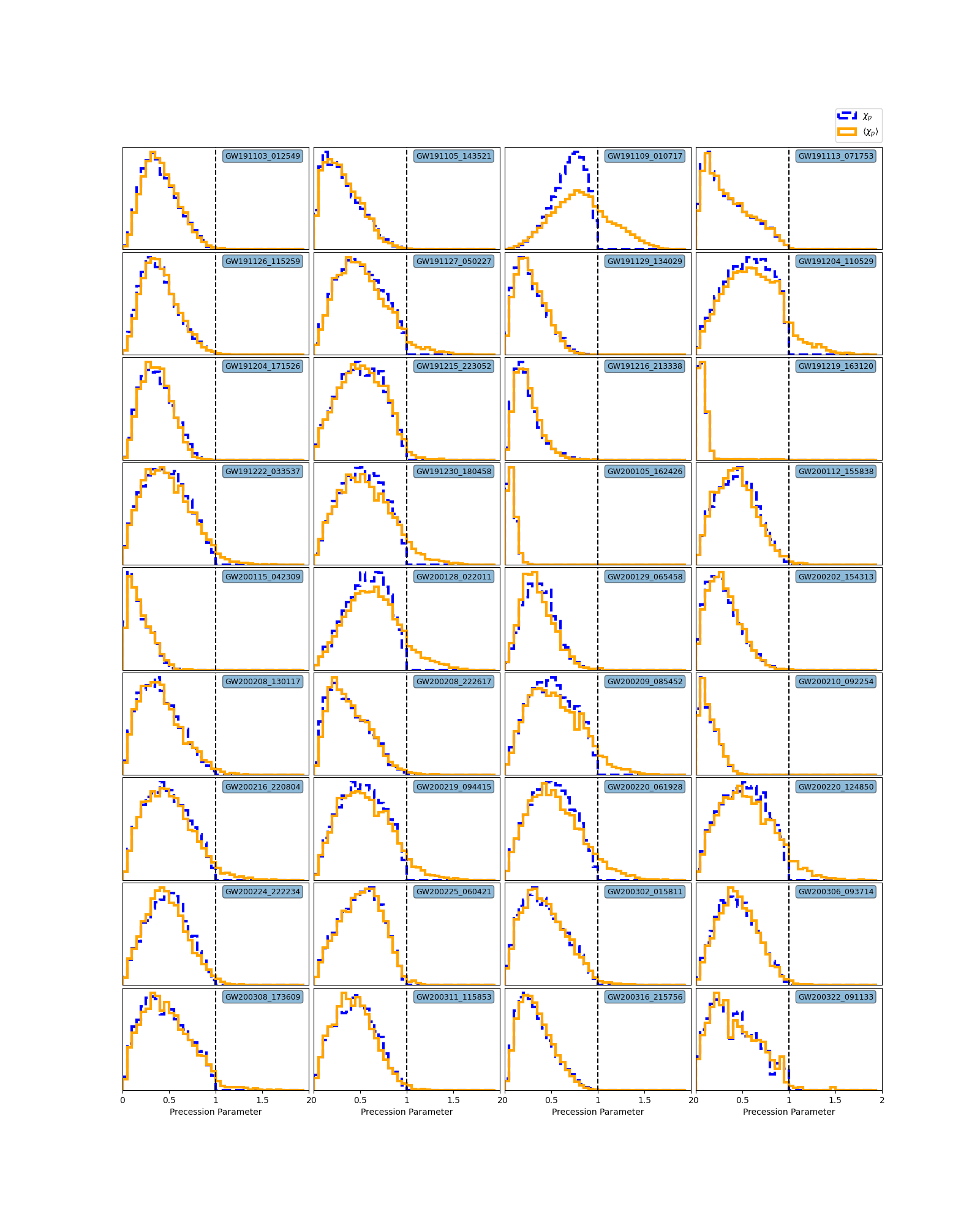
Note that for the majority of these events there are not significant differences in the posterior distributions, as there is not a significant amount of precession. However there are a number of events that have a large probability of being highly precessing, with a parameter peak . The posterior probability distributions for these events show a significant tail in the region, corresponding to the probability that the originating system necessarily contains two misaligned spins.These highly precessing events are show in Fig.(7) with listed in Table(1) below.
| Event | |||
|---|---|---|---|
| GW191109_010717 | 0.28 | ||
| GW191204_110529 | 0.09 | ||
| GW191215_223052 | 0.01 | ||
| GW191230_180458 | 0.07 | ||
| GW200128_022011 | 0.10 | ||
| GW200209_085452 | 0.07 | ||
| GW200219_094415 | 0.06 | ||
| GW200220_061928 | 0.07 | ||
| GW200220_124850 | 0.07 | ||
| GW200225_060421 | 0.01 |
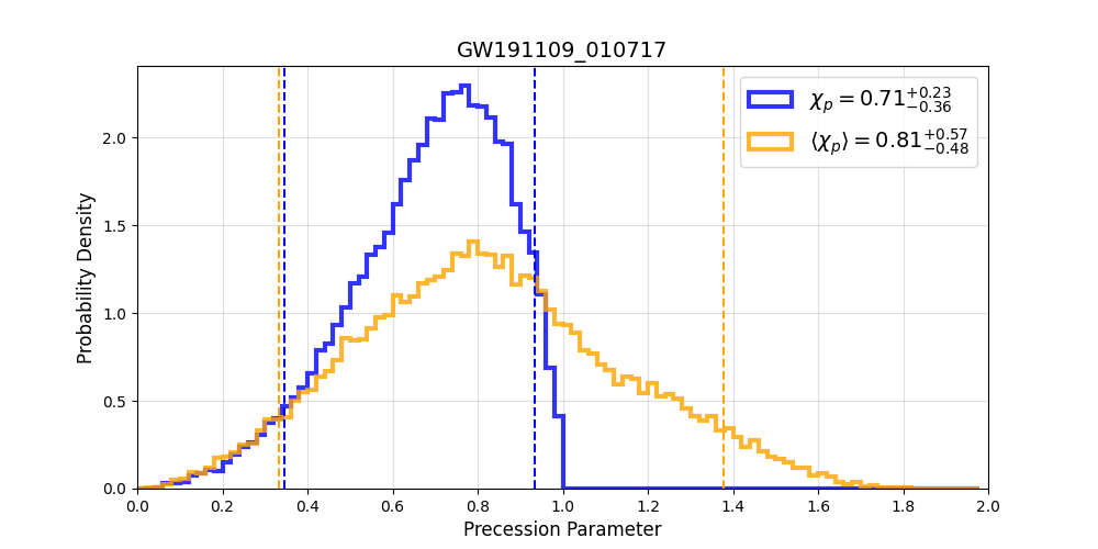
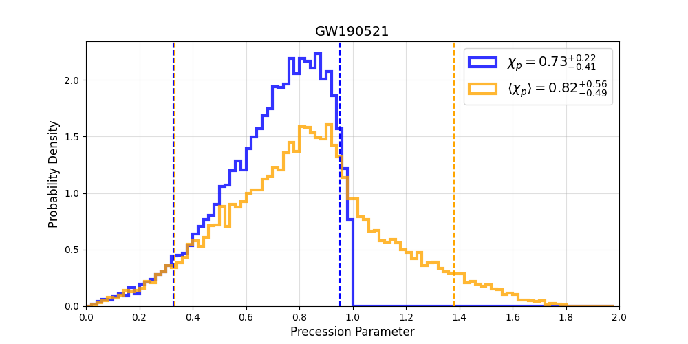
Note that the information about dual-misalignment probability found from calculating is not present from calculating alone. From these initial results we see that for highly precessing events this probability region offers valuable insight into the originating system, as evidence of dual-misaligned systems may contribute to constraining formation channels of precessing systems. Of particular interest is GW191109_010717, shown below in Fig.(5) which presents with a sharply peaked , but a relatively flat distribution of . There are a number of interesting features with this event that can affect the difference in distributions between and .
GW191109_010717 shows component black holes that have dimensionless spin magnitudes of , . The mass ratio of the system is . As discussed in Sec(IV) above, one should expect significant differences between and for a system with two large spin magnitudes and a mass ratio close to unity. Additionally both spins show moderately large probabilities of misalignment, with , . Recall that does not track the misalignment of both objects, only the maximum misalignment, while preserves all the misalignment information. Furthermore, GW191109_010717 is an interesting event due to the total mass. Its constituent black holes have masses of (in the source frame): , , leading to a final black hole of mass . This places the final black hole in the intermediate mass black hole (IMBH) mass range .
There are some remarkable similarities in the precession parameter distributions to those of the salient IMBH candidate event from the first half of the Advanced LIGO and Advanced Virgo third operating run (O3a) , GW190521 [2]. Using parameter estimation data from the public release of GWTC-2 (also without cosmological reweighting), this event also shows a sharply peaked with a that extends significantly into the region, yielding . Similar to GW191109_010717, GW190521 shows component black holes that have dimensionless spin magnitudes of , and a mass ratio of the system is . Thus it also falls into the behavior pattern discussed in Sec(IV). Furthermore this event also shows high total mass, with constituent black holes of (in the source frame) and , leading to a final remnant mass of .
The high total mass of these two events leads to a very short signal duration ( 0.1 s) in the LIGO and Virgo observable band. As pointed out in [33], the short signal duration of GW190521 limits our ability to judge the spin evolution of the system. As such the origin of the difference in distribution of precession parameters as shown in Figs.(5, 6) may be the result of lack of information affecting our ability to characterize precession in IMBH systems. This topic will be addressed in a follow-up paper with further analysis of these two events.
| Event | Event | ||||
| GW191103_012549 | GW200129_065458 | ||||
| GW191105_143521 | GW200202_154313 | ||||
| GW191109_010717 | GW200208_130117 | ||||
| GW191113_071753 | GW200208_222617 | ||||
| GW191126_115259 | GW200209_085452 | ||||
| GW191127_050227 | GW200210_092254 | ||||
| GW191129_134029 | GW200216_220804 | ||||
| GW191204_110529 | GW200219_094415 | ||||
| GW191204_171526 | GW200220_061928 | ||||
| GW191215_223052 | GW200220_124850 | ||||
| GW191216_213338 | GW200224_222234 | ||||
| GW191219_163120 | GW200225_060421 | ||||
| GW191222_033537 | GW200302_015811 | ||||
| GW191230_180458 | GW200306_093714 | ||||
| GW200105_162426 | GW200308_173609 | ||||
| GW200112_155838 | GW200311_115853 | ||||
| GW200115_042309 | GW200316_215756 | ||||
| GW200128_022011 | GW200322_091133 |
VI. Closing Remarks
The precession parameter is a normalized measure of the maximum projection of spin misalignment onto the orbital plane between the two objects in a binary system. As such this parameter takes information from only one object, averaging over only the azimuthal angle difference , and does not account for the variation of the polar angles on the precession timescale . This inconsistency in averaging is resolved by the parameter , which averages over all the angular variations on the precession timescale and preserves the spin-misalignment information from both objects in the binary.
The generalized precession parameter has now been implemented in the parameter estimation algorithm RIFT, and is now available in the latest release of RIFT at https://github.com/oshaughn/research-projects-RIT. With this implementation, both and can be calculated for any set of intrinsic parameters and can therefore be used to generate posterior distributions from existing sample data. Such posteriors can be created and plotted directly from past and future posterior sample data using the plot_posterior_corner.py tool. For more information on using RIFT and associated functions, see https://github.com/oshaughn/RIFT_tutorials. It should be emphasized that the calculation of these parameters presented in this work were not sampled as part of the ILE/CIP process described in Sec.(i). An analysis of this sampling technique and its effect on parameter estimation of precessing systems is planned for future work, along with comparisons to alternative parameterizations of precession and the influence of higher-order waveform modes [34, 35].
Additionally the precession characteristics for all 36 events from GWTC-3 have been reported. It was shown that there are ten events displaying high precession , for which there are significant probabilities that their originating systems necessarily contain two misaligned spins. Further analysis of these events, in particular GW191109_010717, is planned for a follow-up paper.
Acknowledgements
This research has made use of data, software and/or web tools obtained from the Gravitational Wave Open Science Center (https://www.gw-openscience.org/ ), a service of LIGO Laboratory, the LIGO Scientific Collaboration and the Virgo Collaboration. LIGO Laboratory and Advanced LIGO are funded by the United States National Science Foundation (NSF) as well as the Science and Technology Facilities Council (STFC) of the United Kingdom, the Max-Planck-Society (MPS), and the State of Niedersachsen/Germany for support of the construction of Advanced LIGO and construction and operation of the GEO600 detector. Additional support for Advanced LIGO was provided by the Australian Research Council. Virgo is funded, through the European Gravitational Observatory (EGO), by the French Centre National de Recherche Scientifique (CNRS), the Italian Istituto Nazionale di Fisica Nucleare (INFN) and the Dutch Nikhef, with contributions by institutions from Belgium, Germany, Greece, Hungary, Ireland, Japan, Monaco, Poland, Portugal, Spain. This material is based upon work supported by the LIGO Laboratory which is a major facility fully funded by the NSF. The authors are grateful for computational resources provided by LIGO laboratory, supported by NSF Grants PHY-1841475, PHY-2110481, and PHY-2012057. Additional thanks to Richard U’dall for helpful discussions and comments. This paper has LIGO document number P2100434.
References
References
- [1] B. P. Abbott et al. “GWTC-1: A Gravitational-Wave Transient Catalog of Compact Binary Mergers Observed by LIGO and Virgo during the First and Second Observing Runs” In Physical Review X 9.3 American Physical Society, 2019, pp. 31040 DOI: 10.1103/PhysRevX.9.031040
- [2] R. Abbott et al. “GWTC-2: Compact Binary Coalescences Observed by LIGO and Virgo during the First Half of the Third Observing Run” In Phys. Rev. X 11 American Physical Society, 2021, pp. 021053 DOI: 10.1103/PhysRevX.11.021053
- [3] The LIGO Scientific Collaboration et al. “GWTC-2.1: Deep Extended Catalog of Compact Binary Coalescences Observed by LIGO and Virgo During the First Half of the Third Observing Run”, 2021 arXiv:2108.01045 [gr-qc]
- [4] The LIGO Scientific Collaboration et al. “GWTC-3: Compact Binary Coalescences Observed by LIGO and Virgo During the Second Part of the Third Observing Run”, 2021 arXiv:2111.03606 [gr-qc]
- [5] F Acernese et al. “Prospects for observing and localizing gravitational-wave transients with Advanced LIGO , Advanced Virgo and KAGRA” In Living Reviews in Relativity 21, 2018
- [6] J Aasi et al. “Advanced LIGO” In Classical and Quantum Gravity 32.7 IOP Publishing, 2015, pp. 074001 DOI: 10.1088/0264-9381/32/7/074001
- [7] J. Veitch et al. “Parameter estimation for compact binaries with ground-based gravitational-wave observations using the LALInference software library” In Physical Review D 91.4 American Physical Society (APS), 2015 DOI: 10.1103/physrevd.91.042003
- [8] Gregory Ashton et al. “Bilby: A User-friendly Bayesian Inference Library for Gravitational-wave Astronomy” In The Astrophysical Journal Supplement Series 241.2 American Astronomical Society, 2019, pp. 27 DOI: 10.3847/1538-4365/ab06fc
- [9] Jacob Lange, Richard O’Shaughnessy and Monica Rizzo “Rapid and accurate parameter inference for coalescing, precessing compact binaries”, 2018 arXiv:1805.10457 [gr-qc]
- [10] C. Pankow, P. Brady, E. Ochsner and R. O’Shaughnessy “Novel scheme for rapid parallel parameter estimation of gravitational waves from compact binary coalescences” In Phys. Rev. D 92 American Physical Society, 2015, pp. 023002 DOI: 10.1103/PhysRevD.92.023002
- [11] Theocharis A. Apostolatos, Curt Cutler, Gerald J. Sussman and Kip S. Thorne “Spin-induced orbital precession and its modulation of the gravitational waveforms from merging binaries” In Phys. Rev. D 49 American Physical Society, 1994, pp. 6274–6297 DOI: 10.1103/PhysRevD.49.6274
- [12] Lawrence E. Kidder “Coalescing binary systems of compact objects to (post-Newtonian order. V. Spin effects” In Phys. Rev. D 52 American Physical Society, 1995, pp. 821–847 DOI: 10.1103/PhysRevD.52.821
- [13] Steinn Sigurdsson and E. S. Phinney “Dynamics and Interactions of Binaries and Neutron Stars in Globular Clusters” In The Astrophysical Journal Supplement Series 99 American Astronomical Society, 1995, pp. 609 DOI: 10.1086/192199
- [14] Fabio Antonini and Mark Gieles “Merger rate of black hole binaries from globular clusters: Theoretical error bars and comparison to gravitational wave data from GWTC-2” In Physical Review D 102.12 American Physical Society (APS), 2020 DOI: 10.1103/physrevd.102.123016
- [15] Jongsuk Hong et al. “Binary black hole mergers from globular clusters: the impact of globular cluster properties” In Monthly Notices of the Royal Astronomical Society 480.4, 2018, pp. 5645–5656 DOI: 10.1093/mnras/sty2211
- [16] A A Trani, A Tanikawa, M S Fujii, N W C Leigh and J Kumamoto “Spin misalignment of black hole binaries from young star clusters: implications for the origin of gravitational waves events” In Monthly Notices of the Royal Astronomical Society 504.1 Oxford University Press (OUP), 2021, pp. 910–919 DOI: 10.1093/mnras/stab967
- [17] Hans A. Bethe and G. E. Brown “Evolution of Binary Compact Objects That Merge” In The Astrophysical Journal 506.2 American Astronomical Society, 1998, pp. 780–789 DOI: 10.1086/306265
- [18] Ataru Tanikawa, Hajime Susa, Takashi Yoshida, Alessandro A. Trani and Tomoya Kinugawa “Merger Rate Density of Population III Binary Black Holes Below, Above, and in the Pair-instability Mass Gap” In The Astrophysical Journal 910.1 American Astronomical Society, 2021, pp. 30 DOI: 10.3847/1538-4357/abe40d
- [19] K. Belczynski et al. “Evolutionary roads leading to low effective spins, high black hole masses, and O1/O2 rates for LIGO/Virgo binary black holes” In Astronomy & Astrophysics 636 EDP Sciences, 2020, pp. A104 DOI: 10.1051/0004-6361/201936528
- [20] Vassiliki Kalogera “Spin‐Orbit Misalignment in Close Binaries with Two Compact Objects” In The Astrophysical Journal 541.1 American Astronomical Society, 2000, pp. 319–328 DOI: 10.1086/309400
- [21] Davide Gerosa et al. “A generalized precession parameter to interpret gravitational-wave data” In Physical Review D 103.6 American Physical Society (APS), 2021 DOI: 10.1103/physrevd.103.064067
- [22] Benjamin Farr, Evan Ochsner, Will M. Farr and Richard O’Shaughnessy “A more effective coordinate system for parameter estimation of precessing compact binaries from gravitational waves” In Phys. Rev. D 90 American Physical Society, 2014, pp. 024018 DOI: 10.1103/PhysRevD.90.024018
- [23] Patricia Schmidt, Frank Ohme and Mark Hannam “Towards models of gravitational waveforms from generic binaries: II. Modelling precession effects with a single effective precession parameter” In Physical Review D 91.2 American Physical Society (APS), 2015 DOI: 10.1103/physrevd.91.024043
- [24] Davide Gerosa and Michael Kesden “precession: Dynamics of spinning black-hole binaries with python” In Physical Review D 93.12 American Physical Society (APS), 2016 DOI: 10.1103/physrevd.93.124066
- [25] Étienne Racine “Analysis of spin precession in binary black hole systems including quadrupole-monopole interaction” In Physical Review D 78.4 American Physical Society (APS), 2008 DOI: 10.1103/physrevd.78.044021
- [26] Thibault Damour “Coalescence of two spinning black holes: An effective one-body approach” In Physical Review D 64.12 American Physical Society (APS), 2001 DOI: 10.1103/physrevd.64.124013
- [27] Michael Kesden, Davide Gerosa, Richard O’Shaughnessy, Emanuele Berti and Ulrich Sperhake “Effective Potentials and Morphological Transitions for Binary Black Hole Spin Precession” In Physical Review Letters 114.8 American Physical Society (APS), 2015 DOI: 10.1103/physrevlett.114.081103
- [28] LIGO Scientific Collaboration, Virgo Collaboration and KAGRA Collaboration “GWTC-3: Compact Binary Coalescences Observed by LIGO and Virgo During the Second Part of the Third Observing Run — Parameter estimation data release” Zenodo, 2021 DOI: 10.5281/zenodo.5546663
- [29] Rich Abbott et al. “Open data from the first and second observing runs of Advanced LIGO and Advanced Virgo” In SoftwareX 13, 2021, pp. 100658 DOI: https://doi.org/10.1016/j.softx.2021.100658
- [30] Charlie Hoy and Vivien Raymond “PESummary: the code agnostic Parameter Estimation Summary page builder” In SoftwareX 15, 2021, pp. 100765 DOI: 10.1016/j.softx.2021.100765
- [31] Serguei Ossokine et al. “Multipolar effective-one-body waveforms for precessing binary black holes: Construction and validation” In Phys. Rev. D 102 American Physical Society, 2020, pp. 044055 DOI: 10.1103/PhysRevD.102.044055
- [32] Geraint Pratten et al. “Computationally efficient models for the dominant and subdominant harmonic modes of precessing binary black holes” In Phys. Rev. D 103 American Physical Society, 2021, pp. 104056 DOI: 10.1103/PhysRevD.103.104056
- [33] R. Abbott et al. “ Properties and Astrophysical Implications of the 150 Binary Black Hole Merger GW190521 ” In The Astrophysical Journal 900.1, 2020, pp. L13 DOI: 10.3847/2041-8213/aba493
- [34] Lucy M. Thomas, Patricia Schmidt and Geraint Pratten “New effective precession spin for modeling multimodal gravitational waveforms in the strong-field regime” In Physical Review D 103.8, 2021, pp. 1–21 DOI: 10.1103/PhysRevD.103.083022
- [35] Antoni Ramos-Buades, Patricia Schmidt, Geraint Pratten and Sascha Husa “Validity of common modeling approximations for precessing binary black holes with higher-order modes” In Physical Review D 101.10 American Physical Society, 2020, pp. 103014 DOI: 10.1103/PhysRevD.101.103014