Space-time extremes of severe US thunderstorm environments

Abstract

Severe thunderstorms cause substantial economic and human losses in the United States. Simultaneous high values of convective available potential energy (CAPE) and storm relative helicity (SRH) are favorable to severe weather, and both they and the composite variable $\mathrm{PROD}=\sqrt{\mathrm{CAPE}}\times\mathrm{SRH}$ can be used as indicators of severe thunderstorm activity. Their extremal spatial dependence exhibits temporal non-stationarity due to seasonality and large-scale atmospheric signals such as El Niño-Southern Oscillation (ENSO). In order to investigate this, we introduce a space-time model based on a max-stable, Brown–Resnick, field whose range depends on ENSO and on time through a tensor product spline. We also propose a max-stability test based on empirical likelihood and the bootstrap. The marginal and dependence parameters must be estimated separately owing to the complexity of the model, and we develop a bootstrap-based model selection criterion that accounts for the marginal uncertainty when choosing the dependence model. In the case study, the out-sample performance of our model is good. We find that extremes of PROD, CAPE and SRH are generally more localized in summer and, in some regions, less localized during El Niño and La Niña events, and give meteorological interpretations of these phenomena.

Keywords: Bootstrap; Brown–Resnick random field; El Niño-Southern Oscillation; Model selection; Non-stationary extremal dependence; Severe thunderstorm environment.

1 Introduction

Severe thunderstorms cause a substantial fraction of the economic and human losses due to natural disasters in the United States (US), such as those due to the tornadoes experienced across six states on 10–11 December 2021, so it is imperative to have a good understanding of their origins. A severe US thunderstorm is defined as one that produces tornadoes, hailstones over one inch ($2.54$ cm) in diameter, or wind gusts in excess of 50 kts ($1$ kt corresponds to approximately $0.51$ m s^-1). Supercells, which are thunderstorms with a deep and persistent rotating updraft, are responsible for many severe thunderstorm reports (79% of tornadoes, for example, according to Trapp et al., 2005), even though only about 10% of thunderstorms are supercells (Doswell III, 2015).

The available thunderstorm data record is compromised by issues such as observational bias that complicate its use for modelling (Verbout et al., 2006; Allen and Tippett, 2015; Edwards et al., 2018), so it is worthwhile to consider meteorological environments that are conducive to severe thunderstorms. Such storms, especially supercell storms, are more probable in the presence of elevated values of convective available potential energy (CAPE) and of certain measures of vertical wind shear (e.g., Brooks et al., 2003; Brooks, 2013) such as storm relative helicity (SRH), which have been used by weather forecasters and climatologists for more than two decades. High values of the combined variable $\mathrm{PROD}=\sqrt{\mathrm{CAPE}}\times\mathrm{SRH}$ are favorable to severe thunderstorms, and PROD has been used as a proxy of severe thunderstorm activity (e.g., by Tippett et al., 2016; Koch et al., 2021); see for example Brooks et al. (2003, Equation (1)) and Koch et al. (2021, Section 1) for justification for this. In addition to the absence of observational bias, an advantage of using thunderstorm environments as a proxy for thunderstorm reports is that their reanalysis values are available at high and regular spatio-temporal resolution (typically 1^∘ longitude and 1^∘ latitude every hour or three hours), which allows techniques from extreme-value theory and geostatistics to be applied. Among papers that have studied the temporal evolution of the extremes of a quantity similar to PROD over part of the contiguous US are Gilleland et al. (2013), who applied the conditional extreme-value model of Heffernan and Tawn (2004) to $\mathrm{WS}\times W_{\mathrm{max}}$, where WS is a measure of wind shear and $W_{\mathrm{max}}=\sqrt{2\times\mathrm{CAPE}}$, Mannshardt and Gilleland (2013), who fitted the generalized extreme-value (GEV) distribution to the annual maxima of $\mathrm{WS}\times W_{\mathrm{max}}$, and Heaton et al. (2011), who considered, for the same variable, a Bayesian hierarchical extreme-value model based on a Poisson point process. Other studies have investigated the link between ENSO and seasonal or monthly means of environments during winter and spring in the US (Allen et al., 2015; Lepore et al., 2017), or between ENSO and monthly maxima of environments such as PROD, CAPE and SRH (Koch et al., 2021). Gilleland et al. (2013) studied the time evolution of spatial patterns of rather extreme events, but did not incorporate the effect of time in their model or consider pointwise maxima. The other papers mentioned above focus on the influence of time or ENSO at the marginal level (grid point by grid point) only, and, to the best of our knowledge, no article has yet considered the potential influence of these variables or more general time-varying covariates on the spatial dependence of maxima. This issue is nevertheless prominent for risk analysis, and both data and physical arguments suggest that large-scale signals such as ENSO, or seasonality, may affect extremal spatial dependence, for instance through the characteristic dimension of individual extreme events.

In this paper we address this question by using a space-time model that consists, at each time point, of a max-stable field whose dependence structure can evolve as a function of large-scale atmospheric signals or seasonal effects. We use reanalysis data from the North American Regional Reanalysis (NARR), and focus on PROD, CAPE and SRH from 1979 to 2015 over a large rectangle of the contiguous US that contains Tornado Alley, its riskiest region. Max-stable fields (e.g., de Haan, 1984; de Haan and Ferreira, 2006; Davison et al., 2012) provide a natural extension of multivariate extreme-value distributions to the infinite-dimensional setting. They are well-suited to model spatial extremes, as they arise as the only possible non-degenerate limiting random fields of appropriately rescaled pointwise maxima of independent replications of a field. The most commonly used parametric max-stable models are the Smith (Smith, 1990), Schlather (Schlather, 2002), Brown–Resnick (Brown and Resnick, 1977; Kabluchko et al., 2009) and extremal-$t$ (Opitz, 2013) models. Although many models for time-varying marginal (GEV) parameters have been proposed (e.g., Davison et al., 2013, and references therein), to our knowledge, no model for time-varying dependence structure has been developed in the spatial extremes context. Thus, our model fills a gap in the literature while allowing us to deal with a significant practical problem. In the multivariate setting, this issue was tackled by Mhalla et al. (2017), who used a generalized additive model to introduce covariates into the Pickands dependence function (Pickands, 1981) of a max-stable random vector. The modelling of spatial non-stationarity (as opposed to temporal non-stationarity) in the dependence structure of max-stable fields has received slightly more attention. Smith and Stephenson (2009) allowed the covariance matrix of the Smith model to vary across space, whereas Huser and Genton (2016) extended the extremal-$t$ model by taking non-stationary correlation functions for the underlying Gaussian random field, and proposed a max-mixture of max-stable models with spatially dependent weights. Space-varying covariates such as longitude, latitude and elevation, can be incorporated into the correlation functions and the weights.

In our space-time model, when the Brown–Resnick or extremal-t fields are used, we propose to let the parameters (range, smoothness and possible anisotropy parameters) of the variogram or correlation function of their underlying Gaussian field depend on covariates through a general regression function that may involve splines or wavelets. In our application, the time step corresponds to one month and we choose a fractional Brown–Resnick field whose range depends on ENSO and month through a tensor product spline. Such a spline basis captures the interactions between the covariates and allows the ENSO effect to vary from one month to the next. We fit our model using pairwise likelihood (e.g., Padoan et al., 2010) and show by simulation that all parameters can be estimated rather accurately. Furthermore, the out-sample performance of our model is good and our findings have broad meteorological explanations. The range parameter tends to be lower in summer for all regions and variables, although the situation is more subtle for CAPE. The ENSO effect mostly occurs in late winter and spring. The range for PROD is higher during both El Niño and La Niña in the North-East and during El Niño in the South-East. The range is higher during both phases in the South-West and the East for CAPE, and in the West and the North-East for SRH. The extremes of PROD, CAPE and SRH are thus more spatially extensive during both phases in some regions.

We also contribute new methods for inference on max-stable fields. In environmental applications, data may exhibit asymptotic independence and/or weakening dependence, in which case max-stable models are unsuitable, and several subasymptotic models have been proposed to alleviate this (e.g., Huser and Wadsworth, 2019; Huser et al., 2021). One should always assess the validity of max-stable models in applications, and Gabda et al. (2012) and Buhl and Klüppelberg (2016) proposed graphical diagnostics for data with standardized margins. Here we develop a max-stability test that accounts for the unknown margins encountered in practice by approximating the distribution of a specific test statistic under the null hypothesis of max-stability using the bootstrap. Owing to the complexity of our model and the large number of grid points considered, simultaneous estimation of the marginal (GEV) parameters and the dependence parameters of the max-stable field is computationally too intensive, and so we fit the model in two steps: we estimate the GEV parameters, transform the data to standard Fréchet margins and then fit the dependence parameters using pairwise likelihood. We demonstrate that, following a two-step procedure, the estimated Huber (1964) sandwich covariance matrix, henceforth sandwich matrix for brevity, gives poor confidence intervals, and the non-parametric bootstrap gives better coverage. We also show that in such a context model selection using the composite likelihood information criterion (Padoan et al., 2010) is sub-optimal and propose a better criterion using a bootstrap-based estimator of the non-normalized composite Kullback–Leibler divergence.

The test mentioned above does not cast doubt on max-stability as a reasonable working hypothesis for our data. Nor does the $\chi$ function (Coles et al., 1999), and plots of conditional exceedance probabilities do not exhibit weakening dependence with increasing levels, though these diagnostics are rather variable. Thunderstorms tend to be most intense when they take the form of supercells or occur within organized systems such as multicellular thunderstorms, squall lines, or mesoscale convective complexes; see Chapters 8 and 9 of Markowski and Richardson (2010), respectively, for multicellular thunderstorms and supercells and for squall lines and mesoscale convective complexes. Although supercells, for instance, represent only about 10% of thunderstorms (Doswell III, 2015), they lead to many severe thunderstorm reports (e.g., 79% of tornadoes according to Trapp et al. (2005)). All these systems are much more spatially extended than single-cell thunderstorms, which indicates that thunderstorms are not necessarily more localized when their severity increases. Moreover, here we model not severe thunderstorms themselves but conducive environments, and weakening dependence is less expected for such large-scale variables than for the hazards they cause.

The rest of the paper is organized as follows. In Section 2, we outline max-stable fields and their estimation by pairwise likelihood, and present the data and some exploratory analyses. Section 3 details our main methodological contributions: the model, the max-stability test, and the bootstrap-based model selection criterion. Section 4 is dedicated to the case study: we apply the model and methodologies developed in Section 3 to the thunderstorm environment data. Section 5 summarizes our main contributions and findings and gives some future perspectives. Throughout the paper, $\mathcal{X}$ denotes a subset of $\mathbb{R}^{2}$, and $\overset{d}{=}$ and $\overset{d}{\rightarrow}$ denote equality and convergence in distribution, respectively; in the case of random fields, these should be understood as applying to all finite-dimensional distributions.

2 Preliminaries

2.1 Max-stable random fields

A random field $\{G(\bm{s}):\bm{s}\in\mathcal{X}\}$ is said to be max-stable if there exist sequences of functions $\{a_{n}(\bm{s}),\bm{s}\in\mathcal{X}\}_{n\geq 1}>0$ and $\{b_{n}(\bm{s}),\bm{s}\in\mathcal{X}\}_{n\geq 1}\in\mathbb{R}$ such that, for any $n\geq 1$,

$$\left\{\frac{\max_{i=1}^{n}G_{i}(\bm{s})-b_{n}(\bm{s})}{a_{n}(\bm{s})}:\bm{s}\in\mathcal{X}\right\}\overset{d}{=}\left\{G(\bm{s}):\bm{s}\in\mathcal{X}\right\},$$

where $G_{1},\dots,G_{n}$ are independent replicates of $G$. Let $\tilde{T}_{1},\dots,\tilde{T}_{n}$, be independent replications of a random field $\{\tilde{T}(\bm{s}):\bm{s}\in\mathcal{X}\}$. Let $\left\{c_{n}(\bm{s}),\bm{s}\in\mathcal{X}\right\}_{n\geq 1}$ and $\left\{d_{n}(\bm{s}),\bm{s}\in\mathcal{X}\right\}_{n\geq 1}$ be sequences of functions that respectively take values in the strictly positive and real numbers. If there exists a non-degenerate random field $\{G(\bm{s}):\bm{s}\in\mathcal{X}\}$ such that

$$\left\{\frac{\max_{i=1}^{n}\tilde{T}_{i}(\bm{s})-d_{n}(\bm{s})}{c_{n}(\bm{s})}:\bm{s}\in\mathcal{X}\right\}\overset{d}{\rightarrow}\left\{G(\bm{s}):\bm{s}\in\mathcal{X}\right\},\quad n\to\infty,$$ (1)

then $G$ must be max-stable (de Haan, 1984), and this explains the relevance of max-stable fields as models for the pointwise maxima of random fields. If $\{G(\bm{s}):\bm{s}\in\mathcal{X}\}$ is a max-stable field, then, for any $\bm{s}\in\mathcal{X}$, $G(\bm{s})$ has a GEV distribution (e.g., Coles, 2001, Section 3.1) with location, scale and shape parameters $\eta_{\bm{s}}$, $\tau_{\bm{s}}$ and $\xi_{\bm{s}}$. The transformed variable $Z(\bm{s})=\left[1+\xi_{\bm{s}}\{G(\bm{s})-\eta_{\bm{s}}\}/{\tau_{\bm{s}}}\right]^{1/\xi_{\bm{s}}}$ is standard Fréchet distributed, i.e., $\mathbb{P}(Z(\bm{s})\leq z)=\exp(-1/z)$ for $z>0$; max-stable fields having standard Fréchet margins are said to be simple. Max-stable fields are sometimes instead standardized to have Gumbel margins; the Gumbel distribution function with location parameter $\mu$ is $\exp[-\exp\{-(x-\mu)\}]$, $x\in\mathbb{R}$, and the standard Gumbel distribution appears when $\mu=0$.

Any simple max-stable field can be represented as (de Haan, 1984)

$$Z(\bm{s})=\max_{i=1}^{\infty}R_{i}U_{i}(\bm{s}),\quad\bm{s}\in\mathcal{X},$$ (2)

where the $(R_{i})_{i\geq 1}$ are the points of a Poisson point process on $(0,\infty)$ with intensity function $r^{-2}\mathrm{d}r$ and the $(U_{i})_{i\geq 1}$ are independent replicates of a non-negative random field $\{U(\bm{s}),\bm{s}\in\mathcal{X}\}$ such that $\text{E}\{U(\bm{s})\}=1$ for any $\bm{s}\in\mathcal{X}$. Any field defined by (2) is simple max-stable, moreover, and this allows parametric max-stable fields to be constructed, such as the Smith (1990), Schlather (2002), Brown–Resnick (Brown and Resnick, 1977; Kabluchko et al., 2009), and extremal-$t$ (Opitz, 2013) models. The last two are flexible and have been found to capture extremes well, and in Section 4 we use the Brown–Resnick model.

Let $\{\varepsilon(\bm{s}):\bm{s}\in\mathcal{X}\}$ be a centred Gaussian random field with stationary increments and semivariogram $\gamma$. Using $U(\bm{s})=\exp\left[\varepsilon(\bm{s})-\mathrm{Var}\{\varepsilon(\bm{s})\}/2\right]$ in (2), where $\mathrm{Var}$ denotes variance, leads to the Brown–Resnick random field associated with $\gamma$. A popular isotropic semivariogram is $\gamma(\bm{s})=\left(\|\bm{s}\|/\rho\right)^{\alpha}$, $\bm{s}\in\mathcal{X}$, where $\rho>0$ and $\alpha\in(0,2]$ are the range and smoothness parameters, respectively, and $\|\cdot\|$ is the Euclidean distance. Theorem 3.1 of Kabluchko and Schlather (2010) implies that an unbounded semivariogram such as this yields a field that is mixing, which is appropriate if the extreme events are spatially localized. As pointwise maxima typically arise from several individual events, the spatial scale of dependence reflects the extent of the individual extreme events (e.g., Dombry et al., 2018). Thus the range parameter influences the characteristic size of individual extreme events, whereas the smoothness parameter controls the regularity of the field’s sample paths. We will account for possible geometric anisotropy by using the semivariogram

$$\gamma(\bm{s})=\left(\|A\bm{s}\|/\rho\right)^{\alpha},\quad\bm{s}\in\mathcal{X},$$ (3)

where

$$A=\begin{pmatrix}\cos\kappa&-\sin\kappa\\ r\sin\kappa&r\cos\kappa\end{pmatrix},$$ (4)

with scaling and rotation parameters respectively $r>0$ and $\kappa\in[0,\pi]$, which Blanchet and Davison (2011) used to introduce anisotropy into the Schlather model.

The Schlather and extremal-$t$ models are also typically parametrized by a range parameter $\rho>0$ and smoothness parameter $\alpha\in(0,2]$ through the isotropic correlation function $C$ of their underlying standard Gaussian field; the powered exponential, Cauchy and Whittle-Matérn correlation functions are common in applications. In anisotropic cases we consider $C(\|A\bm{s}\|)$ instead of $C(\|\bm{s}\|)$, and then the correlations also depend on $r$ and $\kappa$.

For any simple max-stable field, we have, for $\bm{s}_{1},\ldots,\bm{s}_{D}\in\mathcal{X}$ and $z_{1},\ldots,z_{D}>0$,

$$\mathbb{P}\{Z(\bm{s}_{1})\leq z_{1},\ldots,Z(\bm{s}_{D})\leq z_{D}\}=\exp\left\{-V_{\bm{s}_{1},\ldots,\bm{s}_{D}}(z_{1},\ldots,z_{D})\right\},$$ (5)

with (Pickands, 1981)

$$V_{\bm{s}_{1},\ldots,\bm{s}_{D}}(z_{1},\ldots,z_{D})=\int_{\mathcal{S}_{D}}\max\left\{\frac{w_{1}}{z_{1}},\ldots,\frac{w_{D}}{z_{D}}\right\}\mathrm{d}M_{\bm{s}_{1},\ldots,\bm{s}_{D}}(w_{1},\ldots,w_{D}),$$

where $M_{\bm{s}_{1},\ldots,\bm{s}_{D}}$ is a measure on the $D$-dimensional simplex $\mathcal{S}_{D}$ satisfying

$$\int w_{d}\,\mathrm{d}M_{\bm{s}_{1},\ldots,\bm{s}_{D}}(w_{1},\ldots,w_{D})=1,$$

for each $d\in\{1,\ldots,D\}$. The function $V_{\bm{s}_{1},\ldots,\bm{s}_{D}}$, called the exponent measure of the max-stable random vector $(Z(\bm{s}_{1}),\ldots,Z(\bm{s}_{D}))^{\prime}$, entirely characterizes its dependence and is homogeneous of order $-1$; the  “^′” denotes transposition of a vector. Summaries of the dependence, so-called dependence measures, proposed for max-stable fields/vectors include the extremal coefficient (Schlather and Tawn, 2003). If $Z$ is a simple max-stable field, then the bivariate distribution function satisfies

$$\mathbb{P}(Z(\bm{s}_{1})\leq u,Z(\bm{s}_{2})\leq u)=\exp\left\{-\frac{\theta(\bm{s}_{1},\bm{s}_{2})}{u}\right\},\quad\bm{s}_{1},\bm{s}_{2}\in\mathcal{X},$$ (6)

where $u>0$ and $\theta(\bm{s}_{1},\bm{s}_{2})$ is the bivariate extremal coefficient. By homogeneity of the exponent measure, $\theta(\bm{s}_{1},\bm{s}_{2})=V_{\bm{s}_{1},\bm{s}_{2}}(1,1)$. Furthermore, $\theta(\bm{s}_{1},\bm{s}_{2})\in[1,2]$ for any $\bm{s}_{1},\bm{s}_{2}\in\mathcal{X}$, with values $1$ and $2$ indicating perfect dependence and independence, respectively. The lower the value of $\theta(\bm{s}_{1},\bm{s}_{2})$, the higher the dependence. The pairwise extremal coefficient has a one-to-one relation with the F-madogram (Cooley et al., 2006) and this allows it to be estimated non-parametrically. If $Z$ in (6) is a Brown–Renick field associated with the semivariogram $\gamma$, then (e.g., Davison et al., 2012)

$$\theta(\bm{s}_{1},\bm{s}_{2})=2\Phi\left\{\sqrt{\gamma(\bm{s}_{2}-\bm{s}_{1})}/2\right\},\quad\bm{s}_{1},\bm{s}_{2}\in\mathcal{X},$$ (7)

where $\Phi$ denotes the standard univariate Gaussian distribution function.

If $\{Z(\bm{s}):\bm{s}\in\mathcal{X}\}$ is a simple max-stable field, then (e.g., Davison et al., 2012)

$$\lim_{z\rightarrow\infty}\mathrm{Pr}\{Z(\bm{s}_{1})>z\mid Z(\bm{s}_{2})>z\}=2-\theta(\bm{s}_{1},\bm{s}_{2}),\quad\bm{s}_{1},\bm{s}_{2}\in\mathcal{X}.$$ (8)

Thus, unless $Z$ is standard Fréchet white noise, there exist $\bm{s}_{1},\bm{s}_{2}$ such that the limit in (8) is strictly positive and therefore $Z$ is asymptotically dependent. One can assess the suitability of max-stable models by checking whether the left hand-side of (8) vanishes for different pairs of grid points using tests such as those of Huser and Wadsworth (2019) or those reviewed by de Carvalho and Ramos (2012); see for instance Bacro et al. (2010). However, evidence of asymptotic dependence does not entail suitability of max-stable models, as data may show asymptotic dependence without being max-stable. Another feature that max-stable models cannot capture is weakening dependence at increasing intensity levels, sometimes encountered in finite datasets. In this paper, we use diagnostic plots to look for evidence of this instability, while also explicitly testing the null hypothesis of max-stability; see Sections 3.2 and 4.1. Recently proposed sub-asymptotic models for extremes (Zhang et al., 2022; Huser and Wadsworth, 2019; Huser et al., 2017) offer modelling alternatives if there is good evidence that this limiting assumption is not satisfied.

Let $\bm{s}_{1},\ldots,\bm{s}_{D}\in\mathcal{X}$ denote grid points at which we regularly observe a field of pointwise maxima, which, based on (1), we model by a max-stable field. One way to model the marginal parameters is to borrow strength across space, as is done in the Bayesian hierarchical approach used by Davison et al. (2012). In Section 3.1.2 we shall instead justify modelling the margin at grid point $\bm{s}_{d}$ by a GEV distribution with location, scale and shape parameters $\eta_{\bm{s}_{d}}$, $\tau_{\bm{s}_{d}}$ and $\xi_{\bm{s}_{d}}$. In our setting this entails the estimation of $3\times D$, i.e., $1857$, parameters. Computational considerations make it usual to first estimate these marginal parameters by maximum likelihood, and then to fix them and estimate the dependence parameters of the max-stable field by maximizing the composite log-likelihood. The latter approach, and more specifically the maximum truncated pairwise likelihood estimation used in this paper are discussed in detail in Section 6.1 of the Supplementary Material.

2.2 Data and exploratory analysis

The data we study were used in Koch et al. (2021) and constitute a coarse version of reanalysis data from the North American Regional Reanalysis (NARR). They consist of three-hourly time-series of 0–180 hPa CAPE (J kg^-1) and 0–3 km SRH (m² s^-2) from 1 January 1979 at 00:00 Coordinated Universal Time (UTC) to 31 December 2015 at 21:00 UTC. For consistency, we dropped any data for February 29; this does not impact our findings. The domain considered is a rectangle over the contiguous US from $-110^{\circ}$ to $-80^{\circ}$ longitude and $30^{\circ}$ to $50^{\circ}$ latitude (see Figure 2) containing Tornado Alley (Texas, Oklahoma, Kansas, Nebraska, Iowa and South Dakota), the riskiest region for severe thunderstorms. The resolution is 1^∘ longitude and 1^∘ latitude, leading to 651 grid points in our region; no data are available for 32 grid points over water. We use the time series of CAPE and SRH to build three-hourly time series of $\mathrm{PROD}=\sqrt{\mathrm{CAPE}}\times\mathrm{SRH}$ (m³ s^-3). Finally, as a measure of ENSO, we use monthly values of the Niño-3.4 index (${}^{\circ}\mathrm{C}$) from 1979 to 2015, taken from the ERSSTv5 data set publicly available from the National Oceanic and Atmospheric Administration (NOAA) Climate Prediction Center.

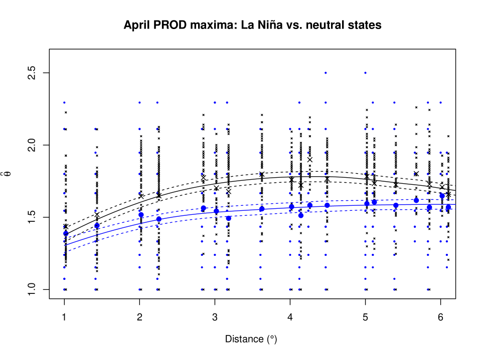
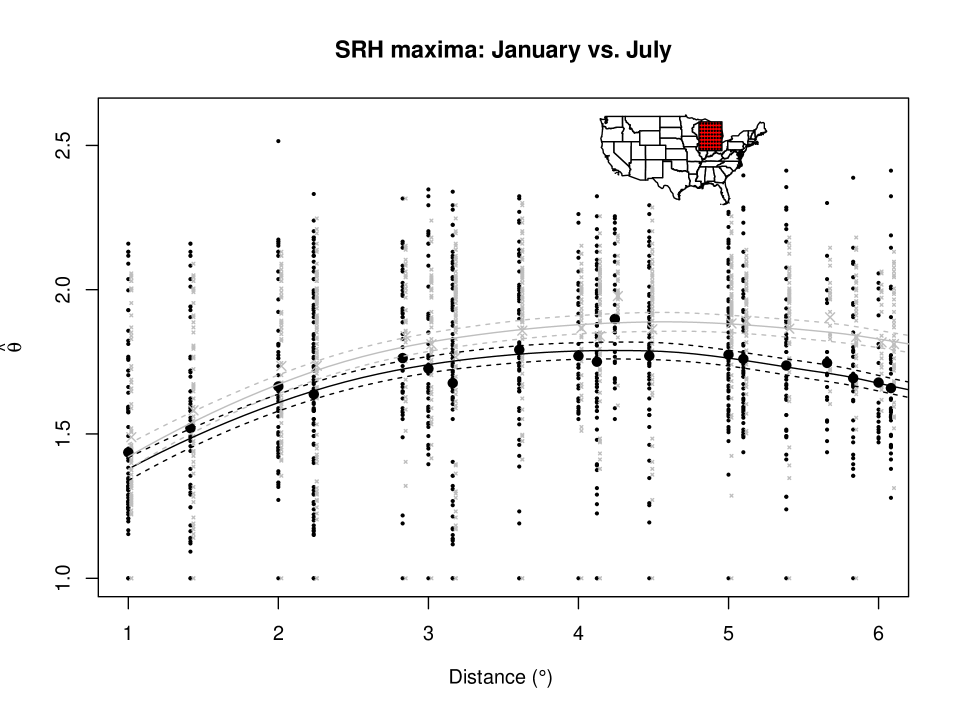
Figure 1 shows that for PROD maxima in April, the bivariate extremal coefficient tends to be lower during La Niña (LN) episodes than during periods with low absolute value of ENSO, indicating that the spatial dependence in the field of pointwise maxima increases during LN events. This may result from an increase of the spatial extent of individual PROD events. Similarly, for SRH maxima, the extremal coefficients are lower in January than in July, suggesting wider SRH events, probably in link with the stronger and more organized jet stream in winter; see Section 4.3. These findings are true for regions other than that used in Figure 1 (not shown) and suggest the use of ENSO and month as covariates when modelling the extremal spatial dependence.

Figure 1: The small dots/crosses show the empirical pairwise extremal coefficients using all grid points in the square indicated by the red region on the map in the right panel, while the larger ones indicate the binned estimates. The solid lines depict the best local polynomial regression curves and the dotted lines characterize the associated $95\%$ pointwise confidence intervals (assuming that the binned estimates are known). The left panel concerns PROD April maxima for $\text{ENSO}<-0.5^{\circ}$C (blue) and $|\text{ENSO}|\leq 0.5^{\circ}$C (black), and the right panel concerns January (black) and July (grey) SRH maxima.

3 Novel methodology

3.1 Model

3.1.1 General case

We propose a space-time model that is simple max-stable at each time point. Let $T$ be the number of time points and let $\bm{x}_{t}=(x_{1,t},\ldots,x_{p,t})^{\prime}$, $t=1,\ldots,T$, gather the observations of $p$ covariates at time $t$, e.g., large-scale atmospheric signals or the month associated with time $t$. Our space-time model $\{Z(\bm{s},t):\bm{s}\in\mathcal{X},t=1,\ldots,T\}$ is then defined as follows:

1. for any $t=1,\ldots,T$, the spatial field $\{Z(\bm{s},t):\bm{s}\in\mathcal{X}\}$ is max-stable with a spatial dependence structure involving the vector of covariates $\bm{x}_{t}$;

2. the spatial fields $\{Z(\bm{s},1):\bm{s}\in\mathcal{X}\},\ldots,\{Z(\bm{s},T):\bm{s}\in\mathcal{X}\}$ are independent.

As mentioned in Section 2.1, max-stable models typically depend on range and smoothness parameters $\rho>0$ and $\alpha\in(0,2]$, a scaling parameter $r>0$ and a rotation parameter $\kappa\in[0,\pi]$. The value of a parameter $a_{t}$ at time $t$ may depend on the $\bm{x}_{t}$ through a linear basis function, viz.

$$g(a_{t})=\sum_{k=1}^{K}\beta_{k}h_{k}(\bm{x}_{t}),$$ (9)

where $g$ is a monotonic link function, $K\in\mathbb{N}\backslash\{0\}$, $h_{1},\dots,h_{K}$ are functions from $\mathbb{R}^{p}$ to $\mathbb{R}$, and the $\beta_{k}$ are real numbers. A convenient choice for $g$ in the case of $\rho$ is the logarithm, but other choices would be necessary for the other parameters. Depending on the choice of $h_{k}$, (9) can represent a generalized linear model or a more flexible and non-linear model (e.g., with splines or wavelets). Radial cubic splines are useful for continuous variables such as weather variables (e.g., ENSO), cyclic P-splines are appropriate when using the month as covariate, as they allow a smooth transition between the first and the last month, and tensor product splines can capture interactions between different covariates. The simultaneous modelling of several parameters with (9) requires enough data, as it can be hard to detect non-stationarity in the dependence structure. For instance, modelling both $\rho$ and $\alpha$ in this way is difficult because their effects may be difficult to distinguish.

3.1.2 Specification for the case study, and simulations

Finding appropriate and parsimonious trend surfaces for the marginal parameters is challenging for large and meteorologically heterogeneous regions. Using ill-specified trend surfaces may bias our characterization of the dependence structure, so we model the monthly maxima by fitting GEV distributions separately at each grid point and then model the field obtained after using these separate fits to transform the data to standard Fréchet margins. Our space-time model for these transformed data lies in the class of max-stable models introduced in Section 3.1.1; we use the Brown–Resnick model with variogram (3), which often fits environmental extremes well (e.g., Davison et al., 2012). Fitting a classical Brown–Resnick model for each month separately showed no evidence of month- or ENSO-specific smoothness, scaling and rotation parameters, for PROD, CAPE or SRH (not shown). Thus, based on our exploratory analysis (Figure 1) and meteorological understanding, we model the range parameter $\rho$ as in (9) with ENSO and month as covariates, keep the parameters $\alpha$, $r$ and $\kappa$ constant, and take the time step to be one month. Our vector of covariates at $t$ is therefore $\bm{x}_{t}=(\mathrm{ENSO}_{t},t\ \mathrm{mod}\ 12)^{\prime}$ and $t=1,\ldots,444$, where $\mathrm{ENSO}_{t}$ is the value of ENSO for the month associated with $t$, and mod denotes the modulo operation. The effect of these covariates on $\rho$ appears to be non-linear (see, e.g., Hoerling et al., 1997, regarding the non-linearity of general responses to El Niño and La Niña), and the covariates interact, so we choose the functions $h_{k}$ as the components of a tensor product spline basis between a radial cubic spline basis in the ENSO direction and a cyclic P-spline basis in the month direction, allowing us to borrow strength from neighbouring ENSO states and months. Thus our final model at time $t=1,\ldots,T$, for the standardized quantities is the Brown–Resnick field with semivariogram

$$\gamma(\bm{s},t)=\left[\frac{\|A\bm{s}\|}{\exp\left\{\sum_{k=1}^{K}\beta_{k}h_{k}(\bm{x}_{t})\right\}}\right]^{\alpha},\quad\bm{s}\in\mathcal{X},$$ (10)

where $A$ is the matrix (4) with $r>0$, $\kappa\in[0,\pi]$, and $K=1$ + number of ENSO knots $\times$ ($1-$ number of month knots). To choose the knots, we fit models with different numbers of knots positioned regularly in each direction and then choose the best using the bootstrap-based selection criterion developed in Section 3.3.

We checked by simulation, detailed in the Supplementary Material, that the model parameters are identifiable and can be estimated adequately in a setting similar to the case study. Such verification is especially important for the model in (10) owing to its complexity and the large number of parameters, and as it is hard to detect non-stationarity in the extremal dependence structure with too few data.

3.2 A max-stability test with unknown margins

Assume that a simple max-stable field $\{Z(\bm{s}):\bm{s}\in\mathcal{X}\}$ is observed in a testing region $\mathcal{T}\subseteq\mathcal{X}$ consisting of grid points $\{\bm{s}_{1},\ldots,\bm{s}_{D}\}$, and let $\mathcal{S}=\{1,\ldots,D\}$. The homogeneity of order $-1$ of the exponent measure in (5) implies that $Z_{\mathcal{S}}=\max_{d\in\mathcal{S}}{\color[rgb]{0,0,0}\log}Z(\bm{s}_{d})$ has a Gumbel distribution with location parameter $\mu_{\mathcal{S}}=\log V_{\bm{s}_{d},d\in\mathcal{S}}$, where $V_{\bm{s}_{d},d\in\mathcal{S}}$ is the value of the exponent measure of $\{Z(\bm{s}_{d}),d\in\mathcal{S}\}$. Gabda et al. (2012) and Buhl and Klüppelberg (2016) visually compared the empirical distribution of $Z_{\mathcal{S}}$ and a Gumbel distribution whose location $\hat{\mu}_{\mathcal{S}}$ has been estimated from simulated realizations of $Z_{\mathcal{S}}$.

In applications we must transform data to standard Fréchet margins before performing such a test. We use the Anderson–Darling (A-D, Anderson and Darling, 1954) statistic to measure the distance between the empirical distribution of $Z_{\mathcal{S}}$ and a Gumbel distribution with location $\hat{\mu}_{\mathcal{S}}$ and thus to assess the null hypothesis that the multivariate distribution is max-stable. The null distribution should allow for the estimation of both $\mu_{\mathcal{S}}$ and the margins, and we use the bootstrap to do so.

Our proposed bootstrap test is parametric for the margins and non-parametric for the dependence, on which we do not wish to impose a particular model. Let $({z}^{\star}_{1,m},\dots,{z}^{\star}_{D,m})^{\prime}$ denote the vector of the $m$-th observed maxima at all grid points in $\mathcal{S}$, where $m\in\{1,\dots,M\}$. For each grid point $d\in\mathcal{S}$, we first fit the GEV distribution using ${z}^{\star}_{d,1},\dots,z^{\star}_{d,M}$ to obtain estimators $\hat{\eta}^{\star}_{d}$, $\hat{\tau}^{\star}_{d}$ and $\hat{\xi}^{\star}_{d}$. We approximate the distribution of the A-D statistic under the null hypothesis of max-stability by $B$ independent replications of the following procedure:

1. use the empirical likelihood-based approach outlined in the Supplementary Material to simulate $M$ replicates of a max-stable vector, denoted $(\tilde{z}_{1,1},\dots,\tilde{z}_{D,1})^{\prime},$ $\dots,$ $(\tilde{z}_{1,M},\dots,\tilde{z}_{D,M})^{\prime}$, such that $\tilde{z}_{d,1},$ $\dots,$ $\tilde{z}_{d,M}$, $d\in\mathcal{S}$, are drawn from a GEV distribution with location, scale and shape parameters $\hat{\eta}^{\star}_{d}$, $\hat{\tau}^{\star}_{d}$ and $\hat{\xi}^{\star}_{d}$. This step uses the total number of underlying observations over all years, $n_{M}=n$ (block size) $\times M$ (number of years), to simulate $M$ replicates of a max-stable vector;

2. for each $d\in\mathcal{S}$, use a GEV distribution fitted to $\tilde{z}_{d,1},\dots,\tilde{z}_{d,M}$ by maximum likelihood to transform the $\tilde{z}_{d,m}$ to approximately standard Fréchet-distributed quantities ${z}_{d,1},\dots,{z}_{d,M}$, yielding $({z}_{1,1},\dots,{z}_{D,1})^{\prime},$ $\dots,$ $({z}_{1,M},\dots,{z}_{D,M})^{\prime}$;

3. compute $z_{\mathcal{S},m}=\max_{d\in\mathcal{S}}{\color[rgb]{0,0,0}\log}z_{d,m}$($m=1,\dots,M$) and fit a Gumbel distribution to $z_{\mathcal{S},1},\dots,z_{\mathcal{S},M}$ using maximum likelihood, giving location parameter estimate $\hat{\mu}_{\mathcal{S}}$;

4. calculate the A-D statistic measuring the distance between the empirical distribution of the $z_{\mathcal{S},1},\dots,z_{\mathcal{S},M}$ and a Gumbel distribution with location $\hat{\mu}_{\mathcal{S}}$.

It is essential to incorporate the uncertainty of the marginal estimation when approximating the distribution of the A-D statistic under the null hypothesis, which we do via Steps 1 and 2 of the procedure. The same test might be applied with $\mathcal{S}$ any subset of $\{1,\dots,D\}$ of size two or more. To assess how our procedure works we perform two experiments detailed in the Supplementary Material, with $D=100$ and $M=40$ block maxima of size $240$, so $n_{M}=40\times 240$.

3.3 Bootstrap-based uncertainty assessment and model selection

Let $\mathcal{Y}=(\bm{Y}_{1},\ldots,\bm{Y}_{T})^{\prime}$ be a data matrix, where $\bm{Y}_{1},\ldots,\bm{Y}_{T}$ are independent replicates of a $D$-dimensional random vector $\bm{Y}$, such as the vector of maxima at certain grid points at a given time, and suppose that the margins of $\bm{Y}$ have been estimated. In this section we discuss uncertainty quantification and model selection when using composite likelihood to estimate the dependence structure.

Suppose we have a parametric model for each margin of $\bm{Y}$ and that the marginal parameters of all components of $\bm{Y}$ are gathered in $\bm{\lambda}$. Below, we consider both the ideal situation where the exact marginal models and $\bm{\lambda}$ are known, and the more realistic situation where $\bm{\lambda}$ is estimated by $\hat{\bm{\lambda}}$ prior to dependence modelling. Let the function $t_{\bm{\lambda}}$ transform a data matrix to have known margins, let $\bm{Z}_{1},\ldots,\bm{Z}_{T}$ and $\bm{Z}$ be transformations of $\bm{Y}_{1},\ldots,\bm{Y}_{T}$ and $\bm{Y}$ to have known margins, and let $\mathcal{Z}=(\bm{Z}_{1},\dots,\bm{Z}_{T})^{\prime}$. Then $\mathcal{Z}=t_{\bm{\lambda}}(\mathcal{Y})$ if $\bm{\lambda}$ is known and $\mathcal{Z}=t_{\hat{\bm{\lambda}}}(\mathcal{Y})$ if $\bm{\lambda}$ is estimated by $\hat{\bm{\lambda}}$.

Assume that we model $\mathcal{Z}$ using a family $\mathcal{F}=\{f(\bm{z},\bm{\psi}):\bm{z}\in\mathbb{R}^{D},\bm{\psi}\in\Psi\subseteq\mathbb{R}^{p}\}$ of density functions with known margins (typically standard Fréchet in the spatial extremes setting) and dependence parameter $\bm{\psi}$. The composite likelihood is $L_{C}(\bm{\psi};\mathcal{Z})=\prod_{t=1}^{T}f_{C}(\bm{\psi};\bm{Z}_{t})$, where $f_{C}$ is defined through the density $f$ and characterizes the composite likelihood (see, e.g., Varin and Vidoni, 2005, Definition 1), and $\hat{\bm{\psi}}$ denotes the maximum composite likelihood estimator. In the case of the truncated pairwise likelihood (see (17) in the Supplementary Material), $f_{C}$ is the sum over all pairs of tapered bivariate densities.

When the true marginal models and $\bm{\lambda}$ are known, under mild regularity assumptions, $\hat{\bm{\psi}}\mathrel{\dot{\sim}}\mathrm{N}_{p}\{\bm{\psi},\text{I}(\bm{\psi})^{-1}\}$ for $T$ large, where the Huber (1964) sandwich information matrix $\text{I}(\bm{\psi})=\text{H}(\bm{\psi})\text{J}(\bm{\psi})^{-1}\text{H}(\bm{\psi})$ with $\text{H}(\bm{\psi})=\text{E}\{-\nabla^{2}_{\bm{\psi}}\log L_{C}(\bm{\psi};\mathcal{Z})\}$ and $\text{J}(\bm{\psi})=\text{V}\{\nabla_{\bm{\psi}}\log L_{C}(\bm{\psi};\mathcal{Z})\}$, $\nabla^{2}_{\bm{\psi}}$ and $\nabla_{\bm{\psi}}$ denote the Hessian and gradient operators with respect to $\bm{\psi}$, and V indicates the covariance matrix operator. Confidence intervals can be based on the sandwich matrix $\hat{\text{H}}(\hat{\bm{\psi}})^{-1}\hat{\text{J}}(\hat{\bm{\psi}})\hat{\text{H}}(\hat{\bm{\psi}})^{-1}$ (Padoan et al., 2010), where

$$\hat{\text{H}}(\hat{\bm{\psi}})=-\nabla_{\bm{\psi}}^{2}\log L_{C}(\hat{\bm{\psi}};\mathcal{Z}),\quad\hat{\text{J}}(\hat{\bm{\psi}})=\sum_{t=1}^{T}\{\nabla_{\bm{\psi}}\log f_{C}(\hat{\bm{\psi}};\bm{Z}_{t})\}\{\nabla_{\bm{\psi}}\log f_{C}(\hat{\bm{\psi}};\bm{Z}_{t})\}^{\prime}.$$

After fitting several models in $\mathcal{F}$ using composite likelihood, it is standard to select that having the highest observed value of $\log L_{C}(\bm{\hat{\psi}},\mathcal{Z})-\text{tr}\{\hat{\text{J}}(\hat{\bm{\psi}})\hat{\text{H}}(\hat{\bm{\psi}})^{-1}\}$ (Varin and Vidoni, 2005), or equivalently the lowest observed value of (Padoan et al., 2010)

$$\text{CLIC}=-2\log L_{C}(\bm{\hat{\psi}},\mathcal{Z})+2\text{tr}\{\hat{\text{J}}(\hat{\bm{\psi}})\hat{\text{H}}(\hat{\bm{\psi}})^{-1}\}.$$ (11)

If $\bm{\lambda}$ has been estimated in a first step, as is often the case in spatial extremal analysis, then use of the estimated covariance matrix and CLIC for uncertainty assessment of $\hat{\bm{\psi}}$ and model selection within $\mathcal{F}$ does not account for estimating the marginal parameters $\bm{\lambda}$. In spatial extremes, the non-parametric bootstrap is often used for uncertainty assessment (Davison et al., 2013, 2018; Huser and Wadsworth, 2019), because researchers are aware of the shortcomings of using the sandwich matrix, but this cannot be said of the use of CLIC for model selection in a two-step setting. Many studies (e.g., Davison et al., 2013, 2018; Huser and Genton, 2016; Huser et al., 2021) do not allow for the estimation of the margins.

In order to account for how marginal estimation affects model selection when using composite likelihood, we propose bootstrap estimation of the non-normalized composite Kullback–Leibler divergence (Varin and Vidoni, 2005). In Section 3.3.1 we suppose that the margins are known and extend the results of Shibata (1997) and Cavanaugh and Shumway (1997) to the composite likelihood setting, and in Section 3.3.2 we define a criterion to account for the marginal effects. Section 3.3.3 illustrates the benefits of this method through a simulation study. We suppress the dependence of $\mathcal{Y}$, $\mathcal{Z}$, and $\hat{\bm{\psi}}$ on $T$ throughout.

3.3.1 Known margins

We assume that $\bm{\lambda}$ in $t_{\bm{\lambda}}$ is known and we seek the best model for $\mathcal{Z}=t_{\bm{\lambda}}(\mathcal{Y})$ by estimating the non-normalized composite Kullback–Leibler divergence from a model to the truth using a non-parametric bootstrap, following what Cavanaugh and Shumway (1997) and Shibata (1997) did for the non-normalized Kullback–Leibler divergence.

Let $g(\bm{z})$, $\bm{z}\in\mathbb{R}^{D}$, be the true density of $\bm{Z}$. The non-normalized composite Kullback–Leibler divergence for a model with density in $\mathcal{F}$ is $d_{T}(\bm{\psi})=\text{E}_{o}\{-\log L_{C}(\bm{\psi};\mathcal{Z})\}$, where $\text{E}_{o}$ is the expectation under $g$. The divergence of the model estimated by maximum composite likelihood (with $\hat{\bm{\psi}}$ as estimated parameter) to the truth is thus

$$d_{T}(\hat{\bm{\psi}})=\text{E}_{o}\{-\log L_{C}(\bm{\psi};\mathcal{Z})\}\mid_{\bm{\psi}=\hat{\bm{\psi}}},$$ (12)

but this cannot be computed unless we know $g$. Varin and Vidoni (2005) showed that a biased estimator of (12) is $-\log L_{C}(\hat{\bm{\psi}};\mathcal{Z})$, and adjusted for the bias with a first-order correction. Now, suppose that $\hat{\bm{\psi}}^{*}$ is a bootstrap replicate of $\hat{\bm{\psi}}$, and let E^∗ denote expectation with respect to the bootstrap distribution of $\hat{\bm{\psi}}$. Arguments similar to those in Cavanaugh and Shumway (1997) imply under the usual regularity conditions that

$$\text{Bias}_{T}^{*}=-2\left[\text{E}^{*}\left\{-\log L_{C}\left(\hat{\bm{\psi}}^{*};\mathcal{Z}\right)\right\}+\log L_{C}\left(\hat{\bm{\psi}};\mathcal{Z}\right)\right]$$ (13)

converges almost surely to the bias of $-\log L_{C}(\hat{\bm{\psi}};\mathcal{Z})$ as $T\rightarrow\infty$. A Monte Carlo estimator from $B$ bootstrap replicates yields a strongly consistent estimator of $\text{Bias}_{T}^{*}$ as $B\to\infty$,

$$\hat{\text{ Bias}_{T}^{\star}}=-\dfrac{2}{B}\sum_{b=1}^{B}\left[-\log L_{C}\left\{\hat{\bm{\psi}}^{*}_{b};t_{\bm{\lambda}}(\mathcal{Y})\right\}+\log L_{C}\left\{\hat{\bm{\psi}};t_{\bm{\lambda}}(\mathcal{Y})\right\}\right].$$ (14)

Thus, a natural estimator of twice the quantity in (12) is

$$\quad-2\log L_{C}\left\{\hat{\bm{\psi}};t_{\bm{\lambda}}(\mathcal{Y})\right\}-2\hat{\text{ Bias}_{T}^{\star}}=\dfrac{1}{B}\sum_{b=1}^{B}\left[{2}\log L_{C}\left\{\hat{\bm{\psi}};t_{\bm{\lambda}}(\mathcal{Y})\right\}-{4}\log L_{C}\left\{\hat{\bm{\psi}}^{*}_{b};t_{\bm{\lambda}}(\mathcal{Y})\right\}\right].$$ (15)

For $T$ and $B$ large enough, model selection based on CLIC and (15) should be equivalent.

3.3.2 Unknown margins

Suppose that $\bm{\lambda}$ in $t_{\bm{\lambda}}$ is estimated by $\hat{\bm{\lambda}}$, and we seek the best model for $\mathcal{Z}=t_{\hat{\bm{\lambda}}}(\mathcal{Y})$ within $\mathcal{F}$. An attractive property of the bootstrap-based estimator of the non-normalized composite Kullback–Leibler divergence developed in Section 3.3.1 is that the effect of estimating the margins can be accounted for. In computing the maximum composite likelihood estimate of $\bm{\psi}$ for the $b$-th bootstrap replicate, we estimate the marginal parameters from the bootstrapped data, yielding an estimate $\hat{\bm{\lambda}}^{*}_{b}$. We make this explicit by writing the estimates $\hat{\bm{\psi}}$ and $\hat{\bm{\psi}}^{*}_{b}$ as functions of $\hat{\bm{\lambda}}$ and $\hat{\bm{\lambda}}^{*}_{b}$, respectively. The expectation $\text{E}^{\star}$ in (13) with respect to the bootstrap distribution of $\hat{\bm{\psi}}$ takes the estimation of the margins into account. Following (15), our criterion for model selection is

$$\text{CLIC}^{\text{b}}=\dfrac{1}{B}\sum_{b=1}^{B}\left[{2}\log L_{C}\left\{\hat{\bm{\psi}}\left(\hat{\bm{\lambda}}\right);t_{\hat{\bm{\lambda}}}(\mathcal{Y})\right\}-{4}\log L_{C}\left\{\hat{\bm{\psi}}^{*}_{b}\left(\hat{\bm{\lambda}}^{*}_{b}\right);t_{\hat{\bm{\lambda}}}(\mathcal{Y})\right\}\right],$$ (16)

and the model minimizing this should be chosen. As a full likelihood is a composite likelihood, this could also be used with full likelihood inference.

The matrices $\hat{\text{H}}(\hat{\bm{\psi}})$ and $\hat{\text{J}}(\hat{\bm{\psi}})$ required for confidence intervals or the $\mathrm{CLIC}$ are often cumbersome to compute, and careful application of pseudo-inverse procedures may be needed if $\hat{\text{H}}(\hat{\bm{\psi}})$ is singular, especially for complex models with many parameters. This further supports the use of $\mathrm{CLIC^{b}}$, whose calculation costs the same as a bootstrap.

Expressions asymptotically equivalent to (13) could be used, as in Shibata (1997, Section 2), leading to different but asymptotically equivalent specifications of $\text{CLIC}^{\text{b}}$.

3.3.3 Simulation study

We perform two experiments with three procedures: $\mathrm{P^{k}}$, in which the correct margins are used when fitting the models and CLIC is used for selection; $\mathrm{P^{u}}$, in which the marginal distributions are supposed to be GEV and estimated in a first step, then transformed before fitting the dependence models and using CLIC for selection; and $\mathrm{P^{b}}$, which is like $\mathrm{P^{u}}$ but uses $\text{CLIC}^{\text{b}}$ in (16) for model selection with a non-parametric block bootstrap ($B=200$), in which each replicate is a block. In each case the dependence models are fitted using the approach of Section 6.1. The first procedure approximates the best that CLIC can do.

In the first experiment, we generated $40$ independent replicates at $D\in\{25,100,225\}$ grid points of a Smith field (Smith, 1990) with common standard Fréchet margins and twice the $2\times 2$ identity matrix as covariance matrix, and used $\mathrm{P^{k}}$, $\mathrm{P^{u}}$ and $\mathrm{P^{b}}$ to choose between an isotropic Smith model labelled SM₀ and a two-parameter Brown–Resnick model labelled BR₁; the latter is over-complex because the Smith field corresponds to the Brown-Resnick field with $\alpha=2$ (e.g., Huser and Davison, 2013). Table 1 shows that $\mathrm{P^{k}}$ correctly chooses SM₀ for any $D$ in around $92\%$ of 200 replications. This figure is much lower for $\mathrm{P^{u}}$ and drops to as low as $20\%$ when $D$ increases, due to unaccounted variation from the estimation of the margins, whereas $\mathrm{P^{b}}$ achieves performance close to that of $\mathrm{P^{k}}$.

In a second experiment with a configuration that could be realistic in an environmental application, we generated $40$ independent replicates at $D\in\{25,100,225\}$ grid points of a Brown–Resnick field with common standard Fréchet margins, $\rho=2$ and $\alpha=1$, and used $\mathrm{P^{k}}$, $\mathrm{P^{u}}$ and $\mathrm{P^{b}}$ to choose between BR₁ and a simpler Brown–Resnick model labelled BR₀ with $\rho=2$ fixed and $\alpha$ estimated. Table 1 shows that $\mathrm{P^{k}}$ correctly chooses BR₀ approximately $84\%$ of the time for any $D$, as would be expected in the full likelihood setting with $n$ large. The frequency of true selection ranges from $28\%$ and $44\%$ with $\mathrm{P^{u}}$, and is much higher (between $76\%$ and $80\%$) for $\mathrm{P^{b}}$.

The paired proportions test (McNemar, 1947) ascribes 5% significance to all tests of differences between $\mathrm{P^{u}}$ and $\mathrm{P^{b}}$ for both experiments (not shown). Thus, if the marginal and dependence parameters have to be estimated in two distinct steps and if composite likelihood is used, we strongly advocate the use of $\mathrm{CLIC^{b}}$, (16), rather than CLIC, (11).

	Pk/$\mathrm{P^{u}}$/Pb
True/Alternative	$D=25$	$D=100$	$D=225$
SM0/BR1	93/82/89	90/54/90	94/20/81
BR0/BR1	84/44/80	84/30/76	85/28/76

Table 1: Frequency (in $\%$, computed over $200$ repetitions) of selection of the true (simpler) model for each experiment, procedure and value of $D$.

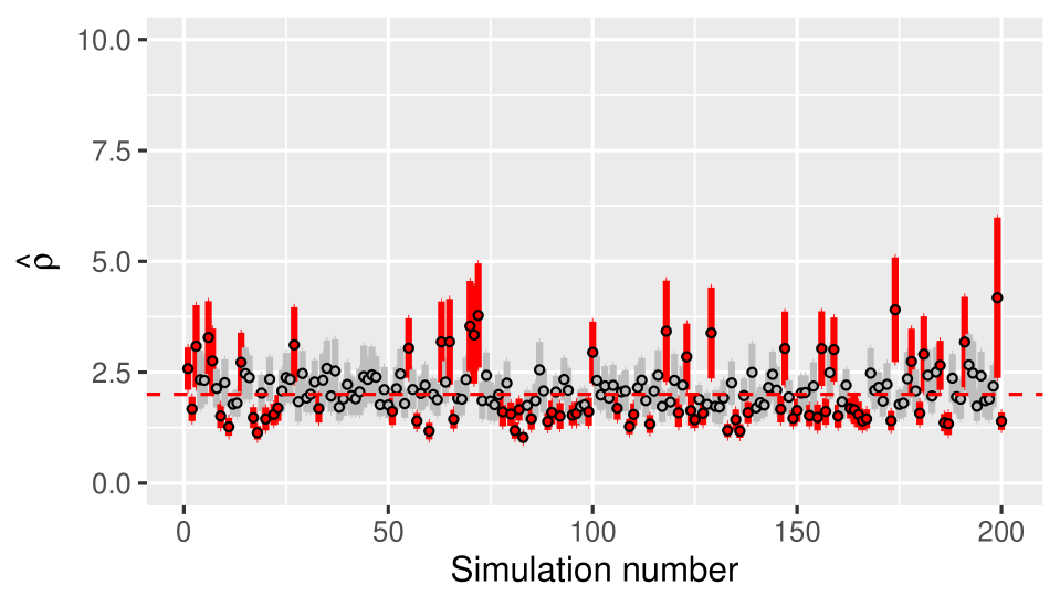
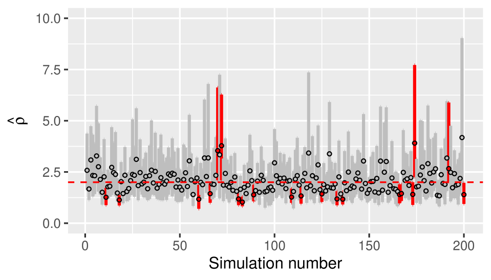
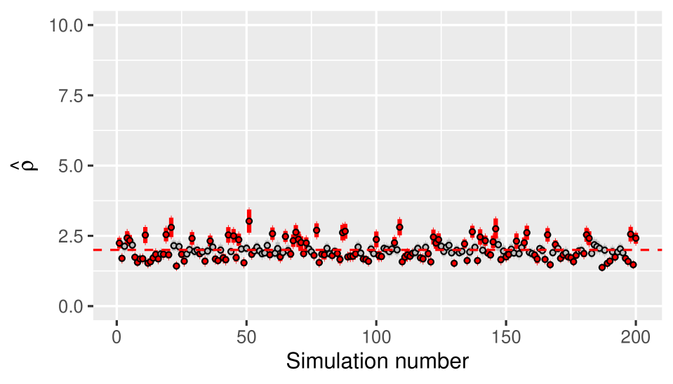
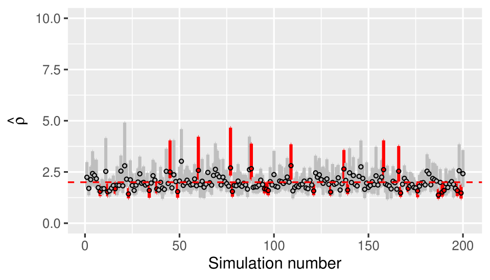
In the second experiment, we also compared the $95\%$ confidence intervals of the range parameter estimates of BR₁ calculated using the sandwich matrix and the non-parametric block bootstrap (Davison and Hinkley, 1997, basic intervals in §5.2) with logarithm as a variance-stabilizing transform; see Figure 12 for $D\in\{25,225\}$. The coverages of the sandwich matrix-based intervals drop from $61\%$ to $39\%$ as $D$ increases from $25$ to $225$, whereas the corresponding values for the bootstrap-based intervals are $90\%$ and $85\%$, lower than the nominal level but not catastrophically so.

4 Case study

4.1 Choice of appropriate regions and max-stability

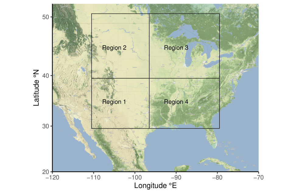
We divide the domain of interest into four regions displayed in Figure 2, and study them separately. These four regions are homogeneous in terms of climate according to the Köppen–Geiger classification (e.g., Beck et al., 2018) and main weather drivers (e.g., in terms of position with respect to the polar and subtropical jet streams). Applying our model to each region (rather than to the full spatial domain) allows us to partially account for the spatial non-stationarity of the dependence structure, and to get finer meteorological interpretations. Moreover, a partition similar to that based on the climate considerations was also obtained by applying o the full domain the clustering method of Bernard et al. (2013), which is suited to maxima and designed to find the groups that are the most independent; see Figure 13 (Supplementary Material). This further supports our split and implies that for our purposes the four regions can be treated separately.

Diagnostic plots (Figures 15 and 16 of the Supplementary Material) showed no evidence that a max-stable model is inappropriate, though these plots use non-parametric estimators that typically give inflated uncertainties near the boundaries. Rather than relying only on these plots, we applied the max-stability test outlined in Section 3.2.

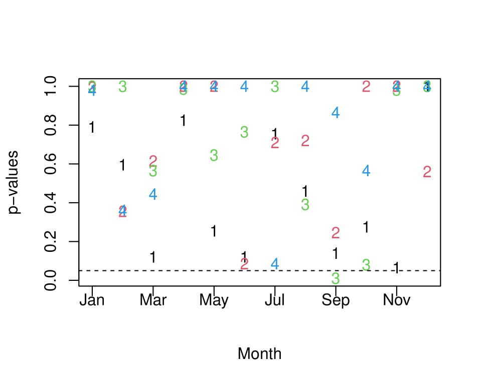
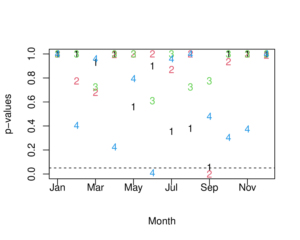
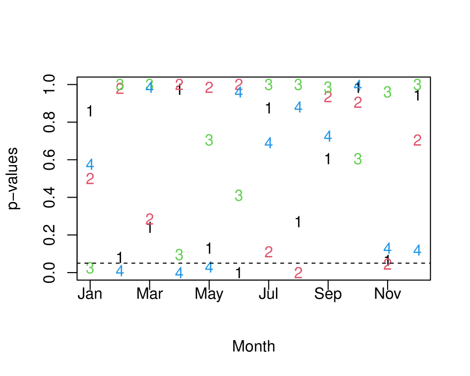
For each variable and each month, we applied our proposed test to each region. Figure 14 (Supplementary Material) suggests that a max-stable model is reasonable, as the number of p-values below a certain level, e.g., 0.05, is reasonable given the number of tests. Nevertheless, Region 4 has a larger number of small $(<0.2)$ p-values for SRH, suggesting that closeness to max-stability varies across space. It also seems to vary seasonally: small p-values often correspond to summer to early winter (e.g., June to November) for PROD, late summer (e.g., September) for CAPE, and winter and spring (e.g., November to May) for SRH. We stress, however, that the power of the test depends heavily on the dependence strength in each region, as shown in the simulation study of Section 3.2.

Figure 2: The partition of the study domain into four regions.

4.2 Results

Regions 1–4 (R1–R4 in the following) respectively contain 140, 154, 164, and 161 grid points. To fit our model, we randomly chose approximately two thirds of the grid points in each region (105, 116, 123, and 121) and validated our models with the rest. The calibration and validation sets are the same for all variables.

We applied the model described in Section 3.1.2 separately to each of the four regions, with $k_{1}\in\{2,3,4\}$ knots in the ENSO direction and $k_{2}\in\{4,5\}$ knots in the month direction. The knots for ENSO are placed evenly between the $10\%$ and $90\%$ quantiles of its values, i.e., between $-1.06^{\circ}$C and $1.16^{\circ}$C, and those for months are positioned evenly between $0.5$ and $12.5$, both of which represent mid-December. We also fitted a range parameter with no covariates. We fitted all models to the calibration set using the truncated pairwise likelihood approach described in Section 6.1 (Supplementary Material).

We assessed the uncertainty of our estimates with basic parametric bootstrap confidence intervals, keeping the covariate information fixed for $200$ replicates; Gilleland (2020) show that the parametric bootstrap is suitable in the context of univariate extreme-value theory. For the range parameter, we used the logarithm as a variance-stabilizing transformation (Davison and Hinkley, 1997, p. 195) and derived the basic confidence intervals for $\log$ range before transforming them back to the original scale. For model selection, we used $\text{CLIC}^{\text{b}}$ in (16) with the same bootstrap replicates.

Table  2 shows that the best models for PROD, CAPE and SRH vary with the region considered: for instance, the best for PROD has three and four knots in the ENSO and month directions in R1, but four and five in R3. These models outperform that with constant range (not shown), suggesting that incorporating ENSO and the month is valuable. Models other than those chosen, especially the more complex ones, lead to similar conclusions in terms of influence of EN and LN (not shown), but considering more knots increases the uncertainty on the parameter estimates (not shown). Below, by ‘model’ we mean the best model for each of SRH, CAPE and PROD.

	PROD				CAPE				SRH
Knots	R1	R2	R3	R4	R1	R2	R3	R4	R1	R2	R3	R4
$2\times 4$	98	226	3031	0	2043	614	6582	1356	978	3495	1570	982
$3\times 4$	0	0	1457	531	1028	477	1566	230	585	162	228	99
$4\times 4$	23	294	1371	540	946	0	1316	0	0	0	352	309
$2\times 5$	227	337	2024	573	692	872	5300	1810	970	2938	1239	0
$3\times 5$	292	521	113	1238	102	950	0	116	733	367	308	271
$4\times 5$	43	543	0	957	0	354	244	255	127	231	0	118

Table 2: Values of $\mathrm{CLIC^{b}}$ for regions R1-R4 and for different configurations $k_{1}\times k_{2}$, where $k_{1}$ and $k_{2}$ are the number of knots in the ENSO and month directions, respectively.

The estimates of the smoothness parameter $\alpha$ shown in Figure 3 suggest that the models for PROD are slightly rougher than those for CAPE, which in turn are slightly rougher than those for SRH. A slight systematic downward bias for $\alpha$ was corrected using the bootstrap replicates. The estimates of the parameters in (4) show a non-negligible compression in the longitude direction ($r$ ranges from $0.5$ to around $0.7$) for all variables for R2, R3 and R4. For all variables, the rotation $\kappa$ is positive for R1 and R2 and negative for R3 and R4.

Figure 3: Bootstrap bias-corrected parameter estimates with their $90\%$ bootstrap confidence intervals for each region and variable.

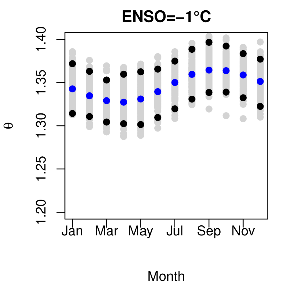
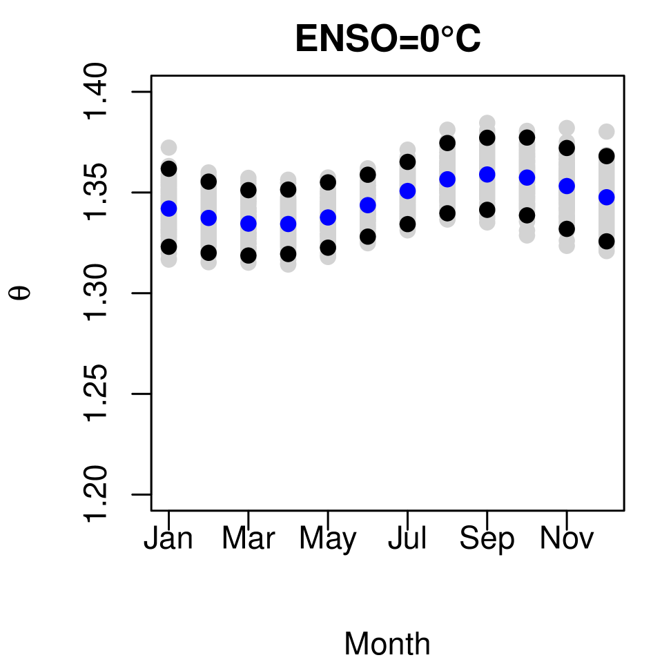
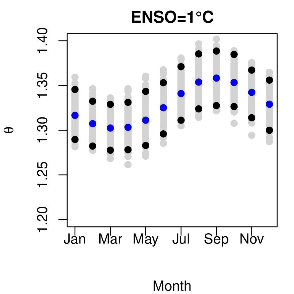
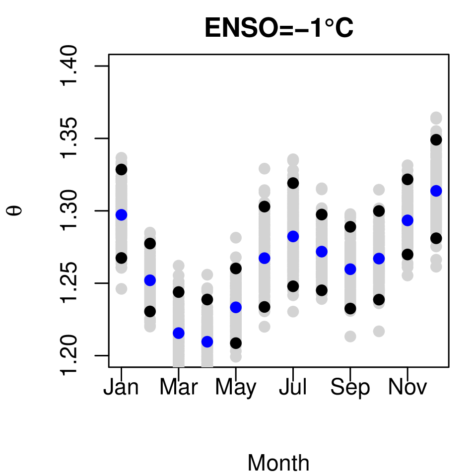
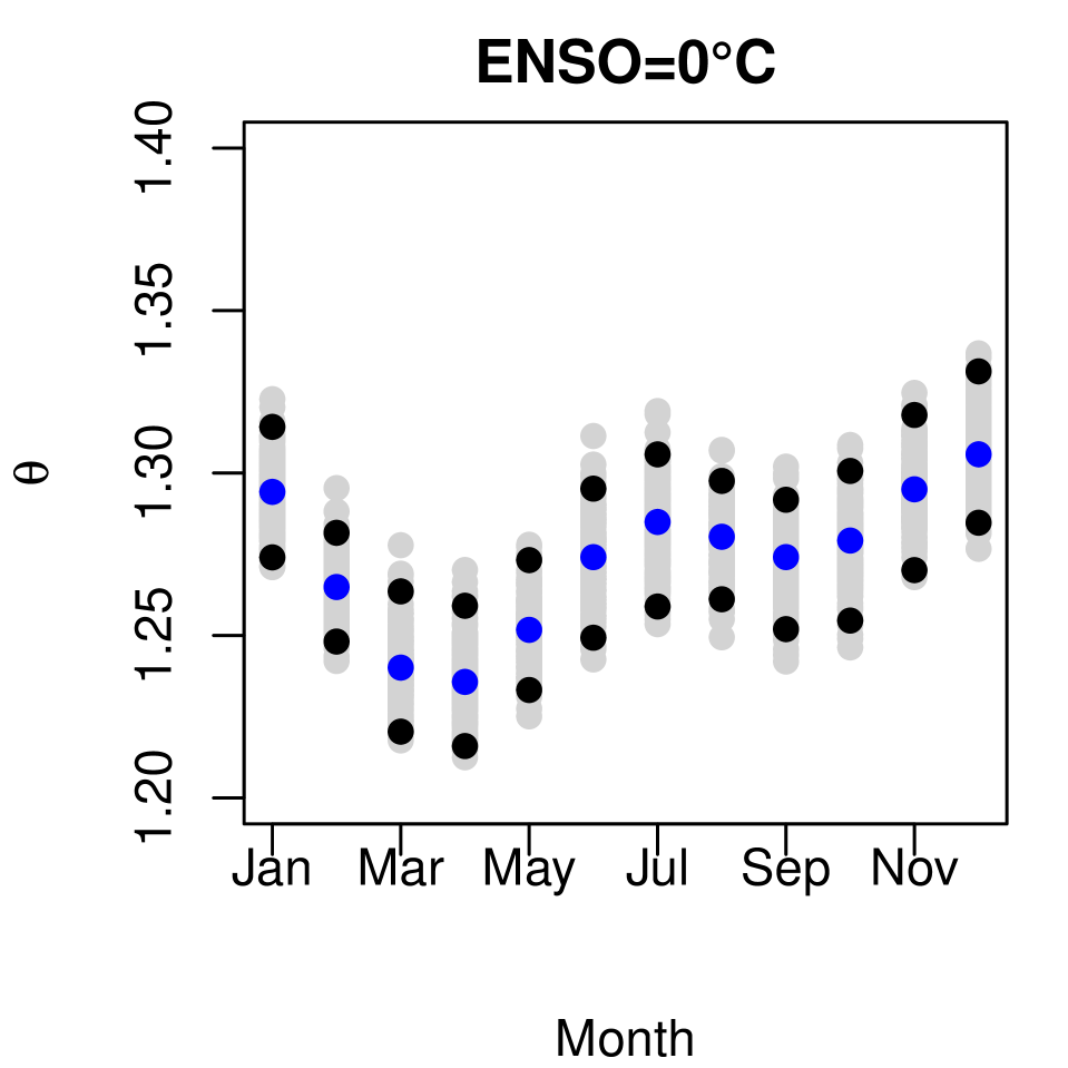
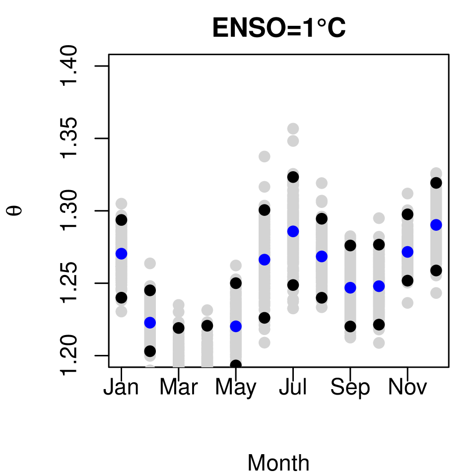
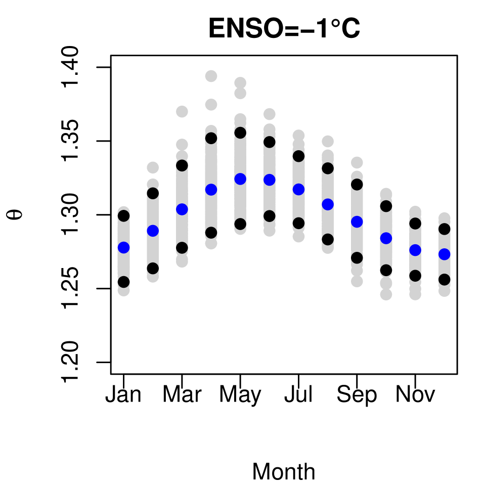
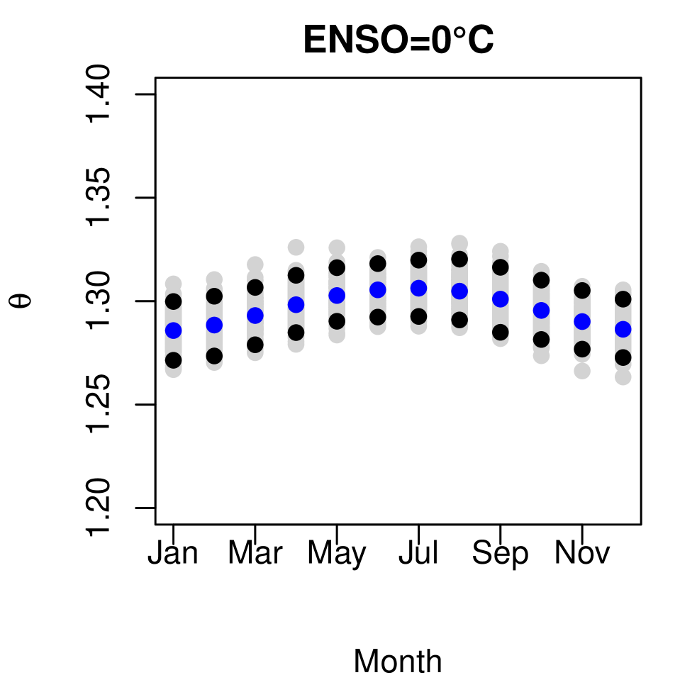
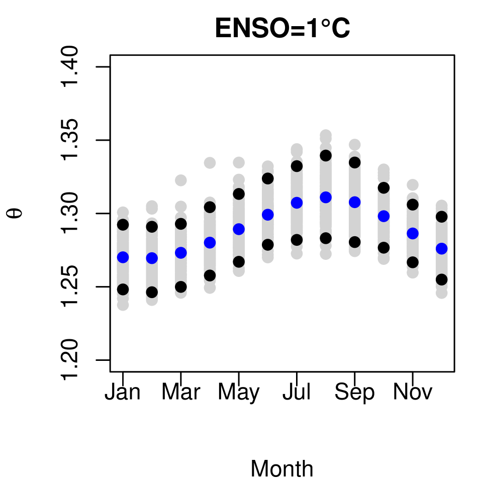
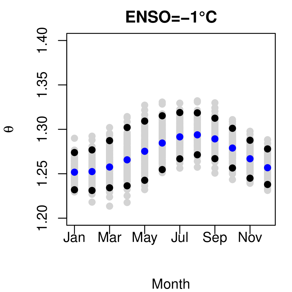
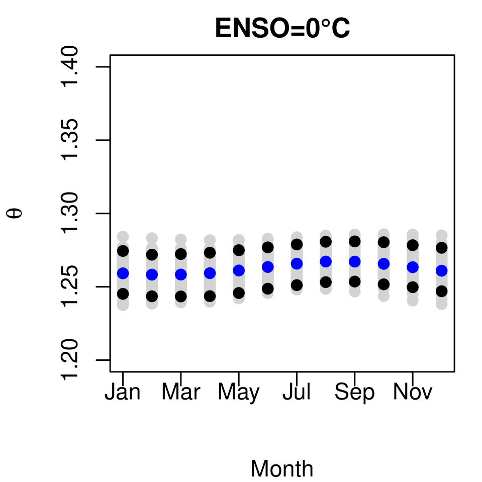
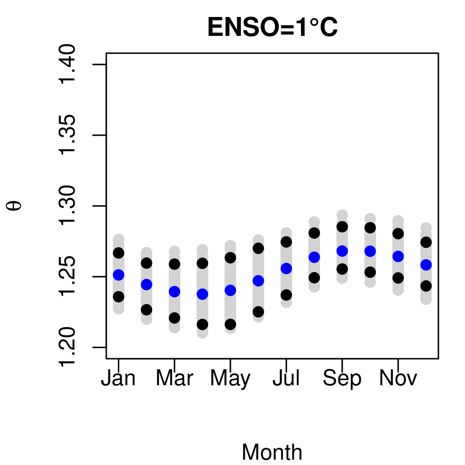
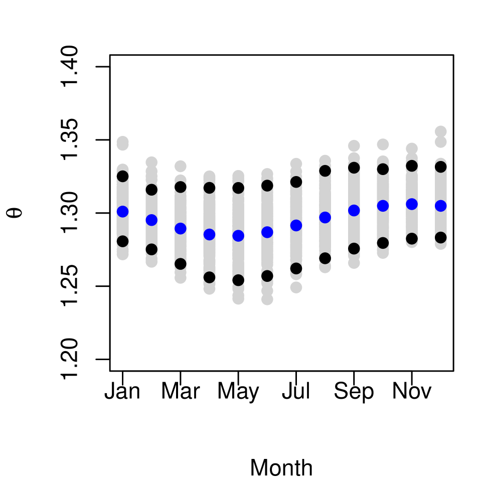
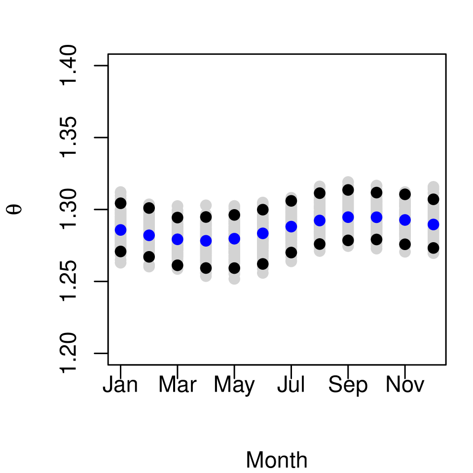
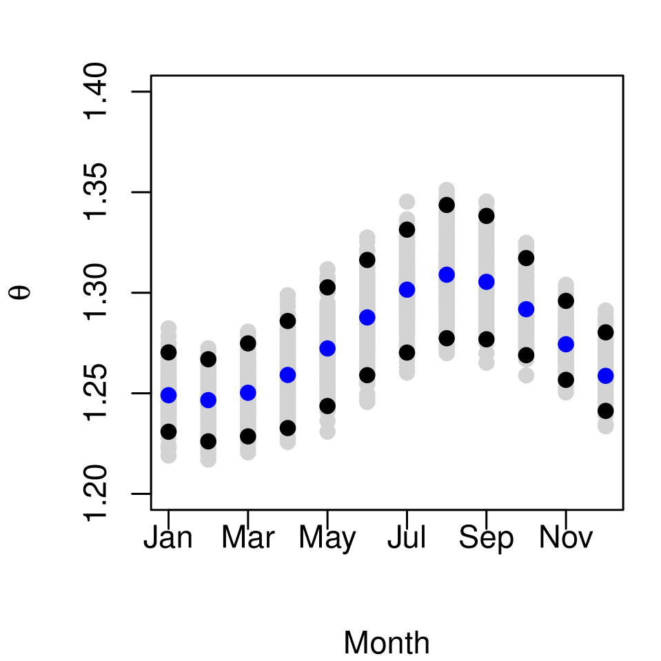
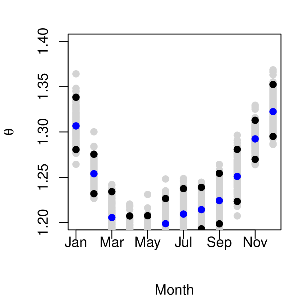
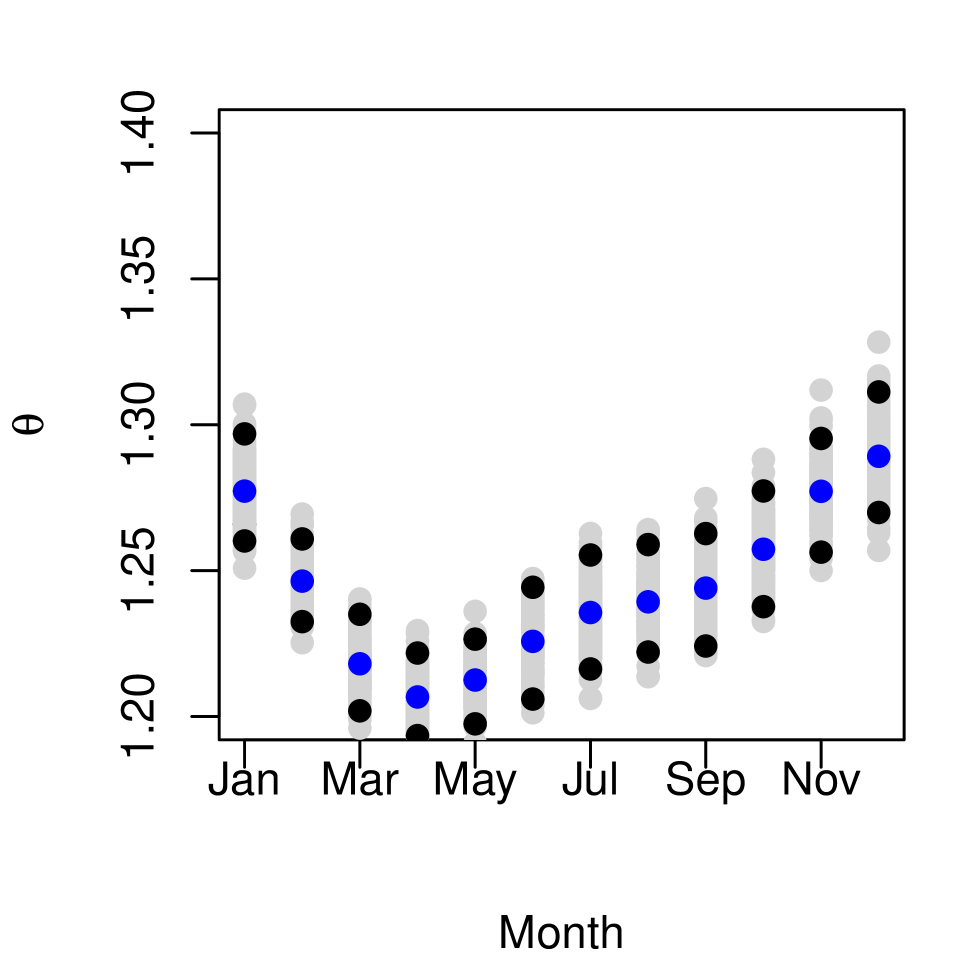
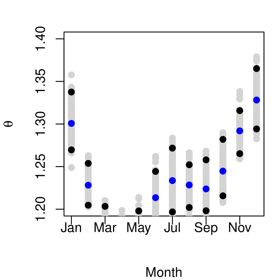
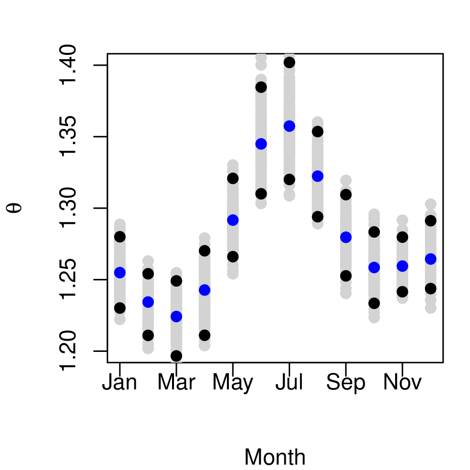
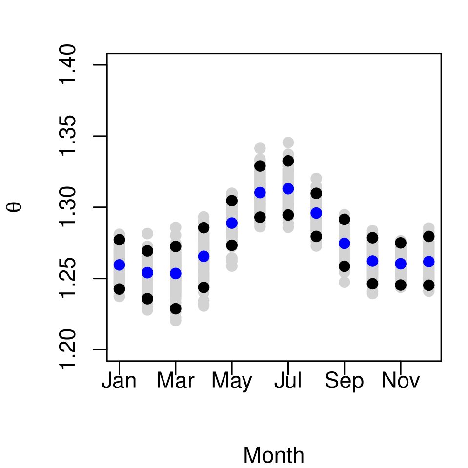
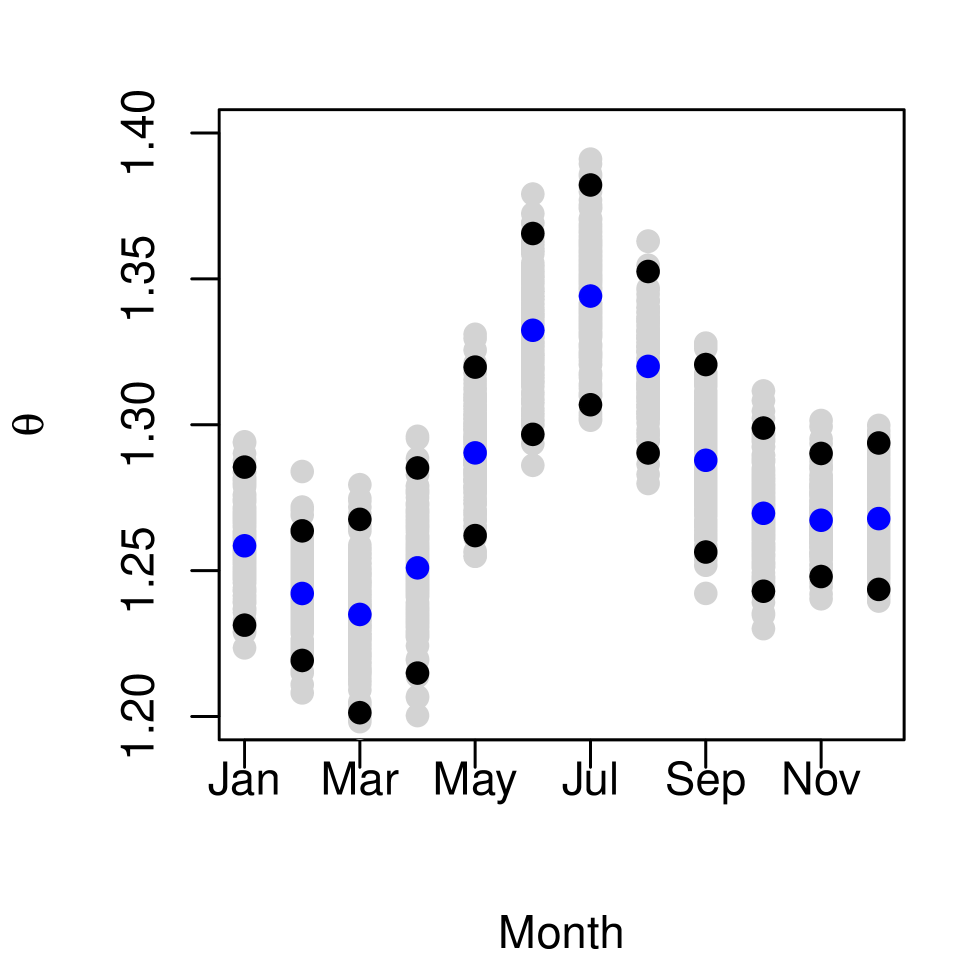
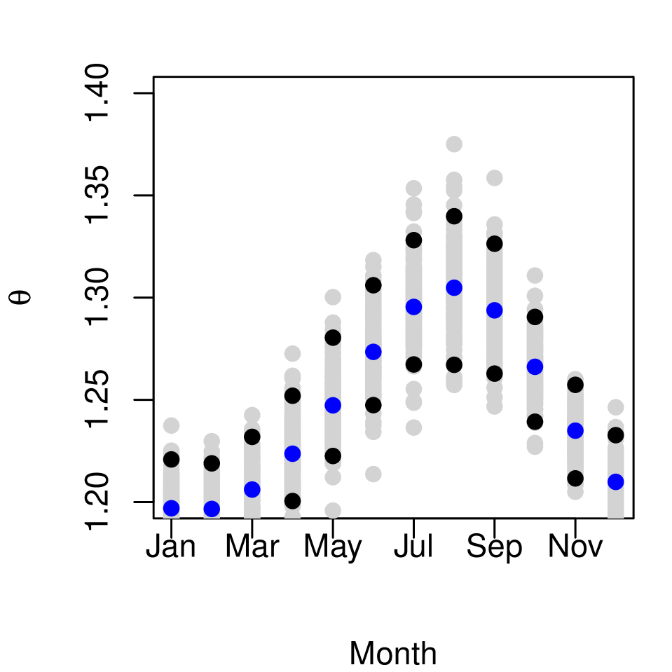
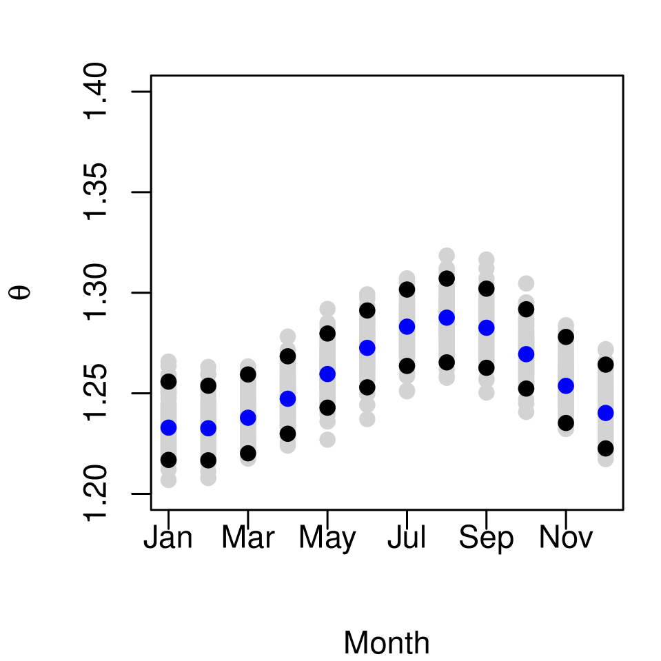
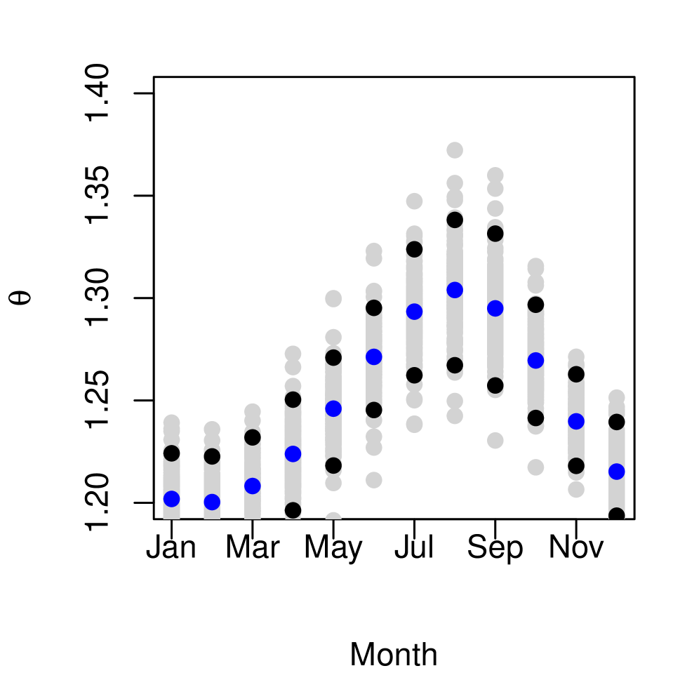
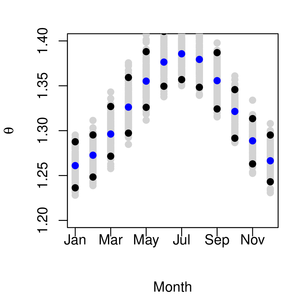
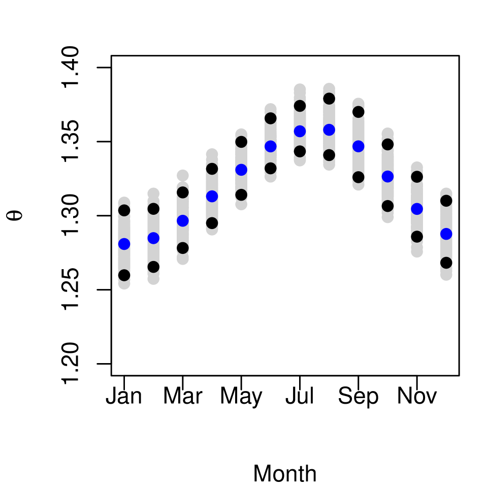
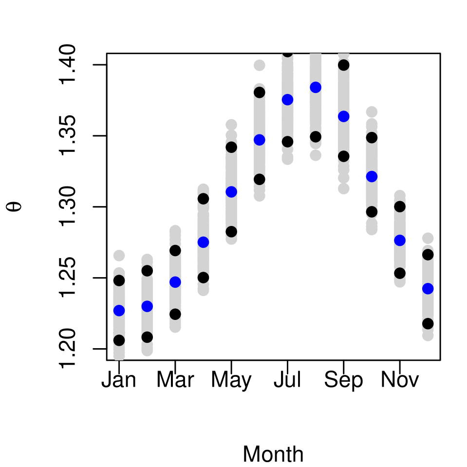
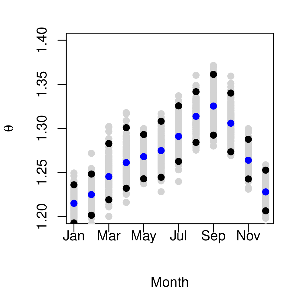
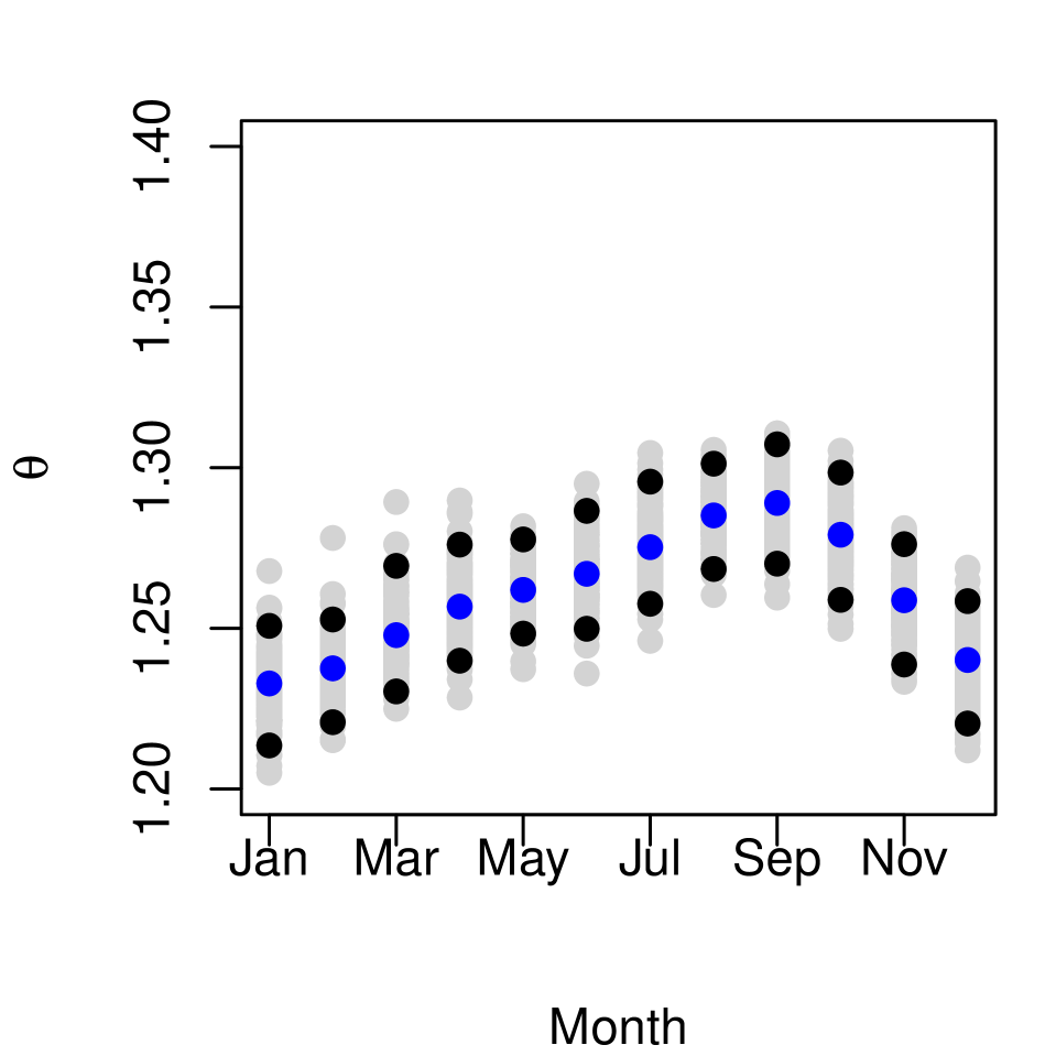
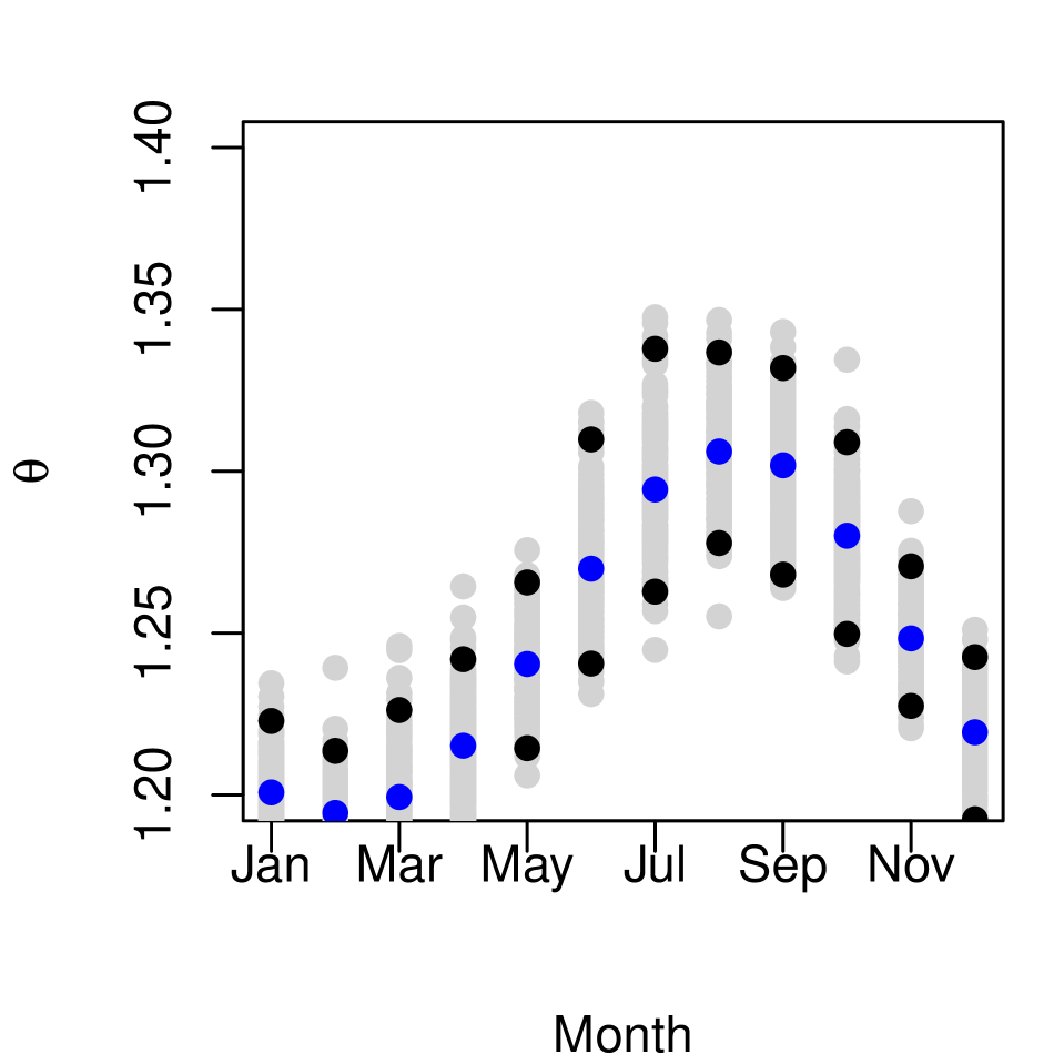
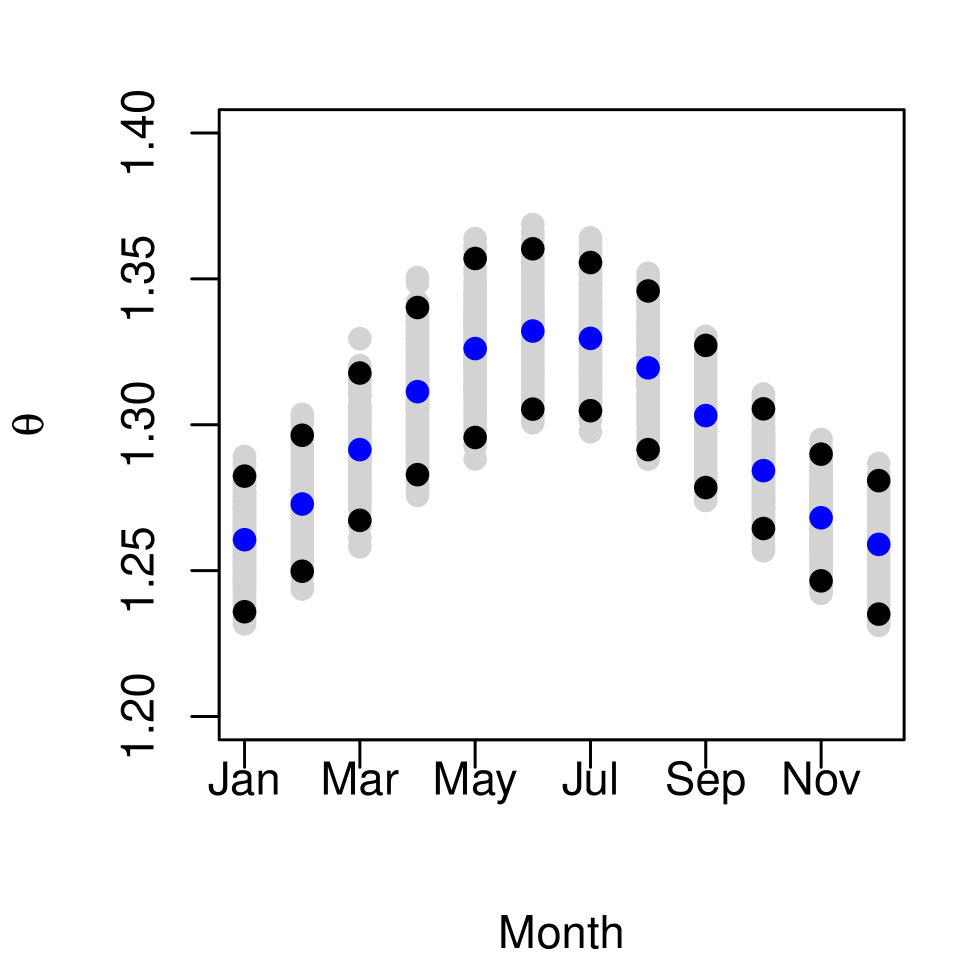
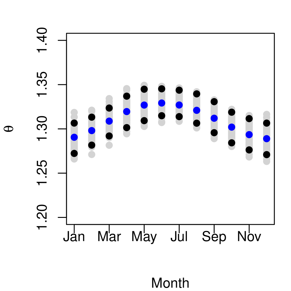
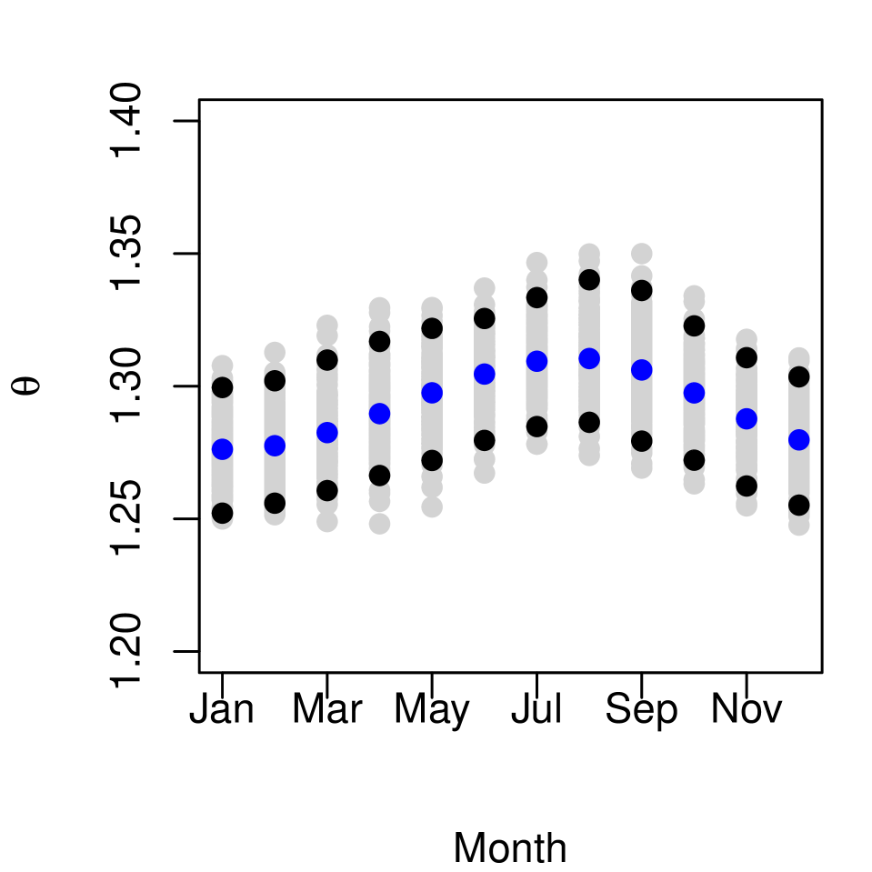
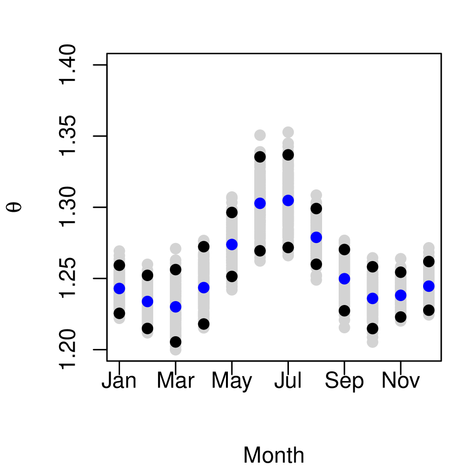
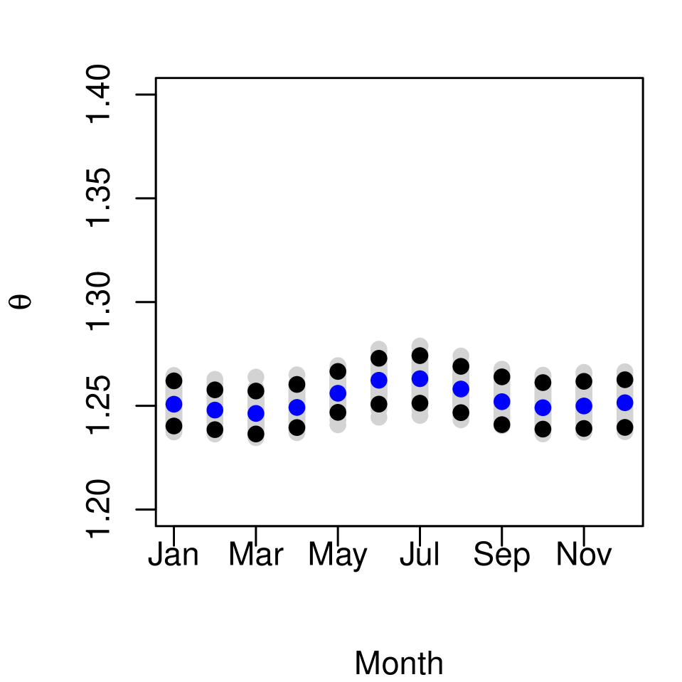
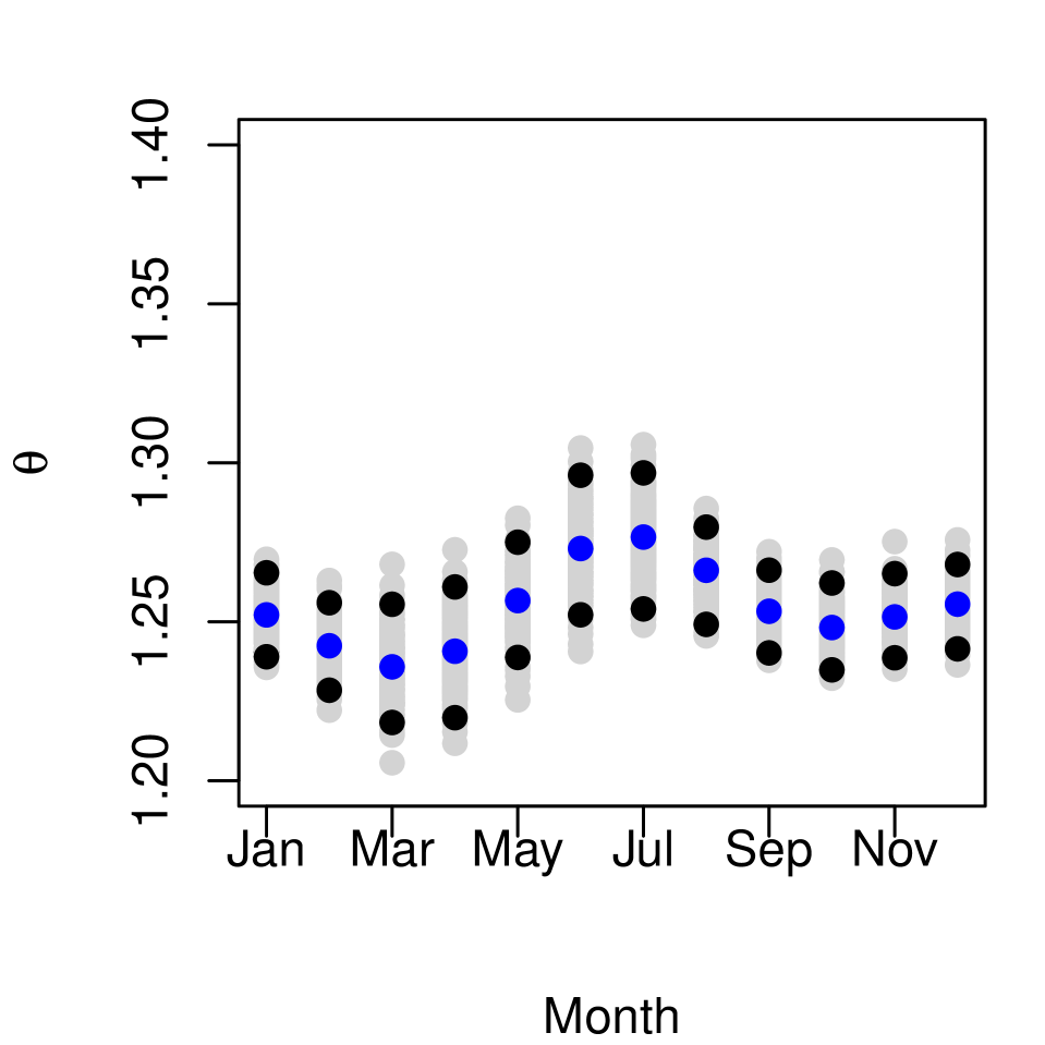
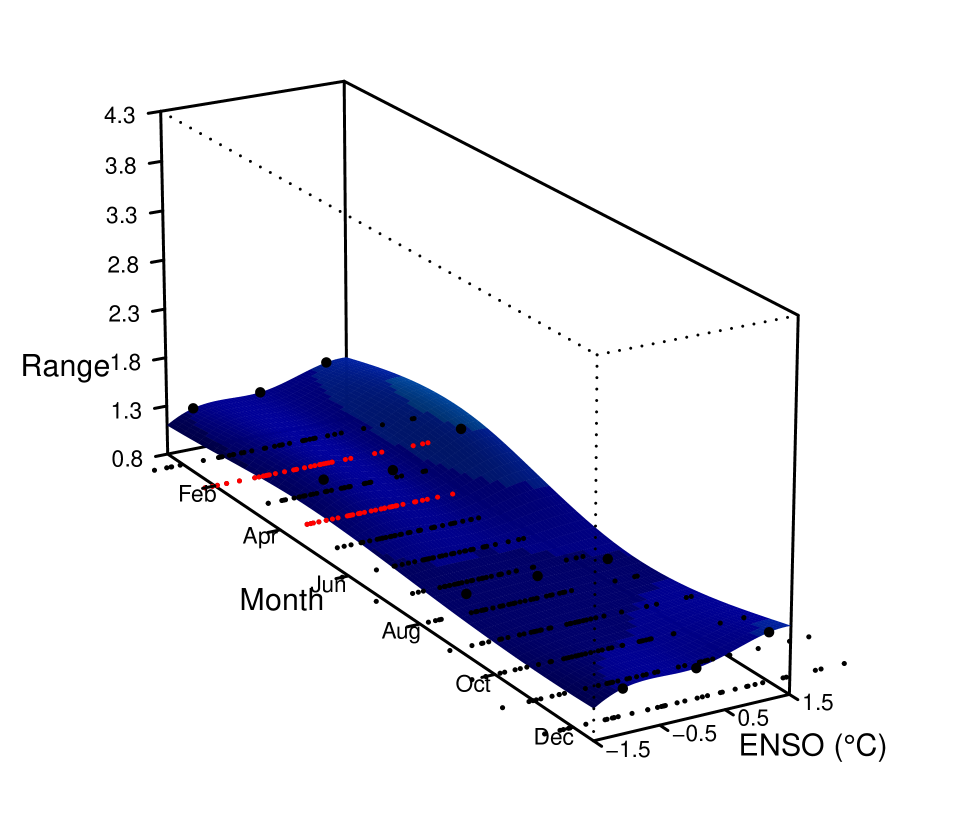
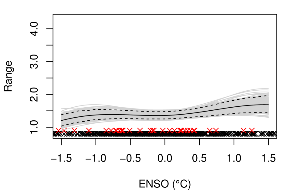
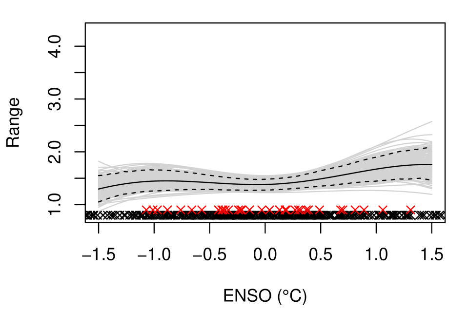
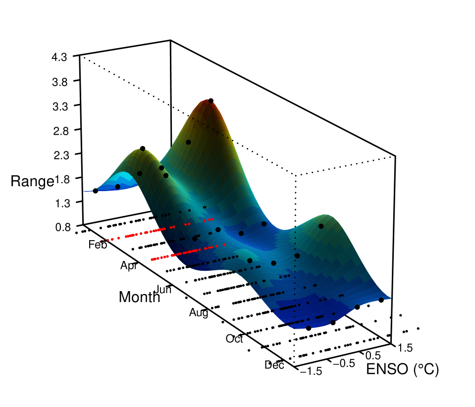
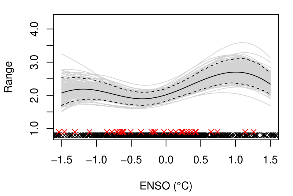
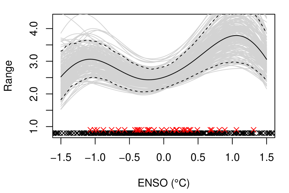
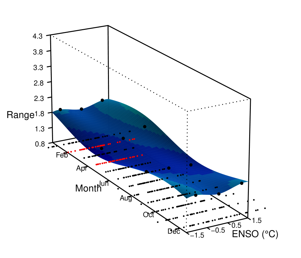
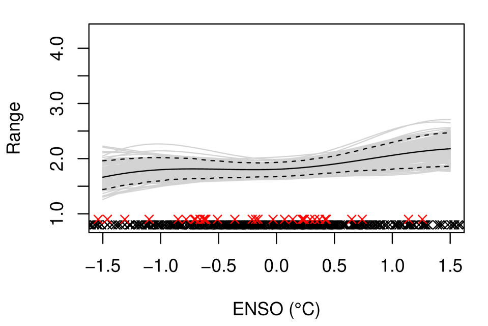
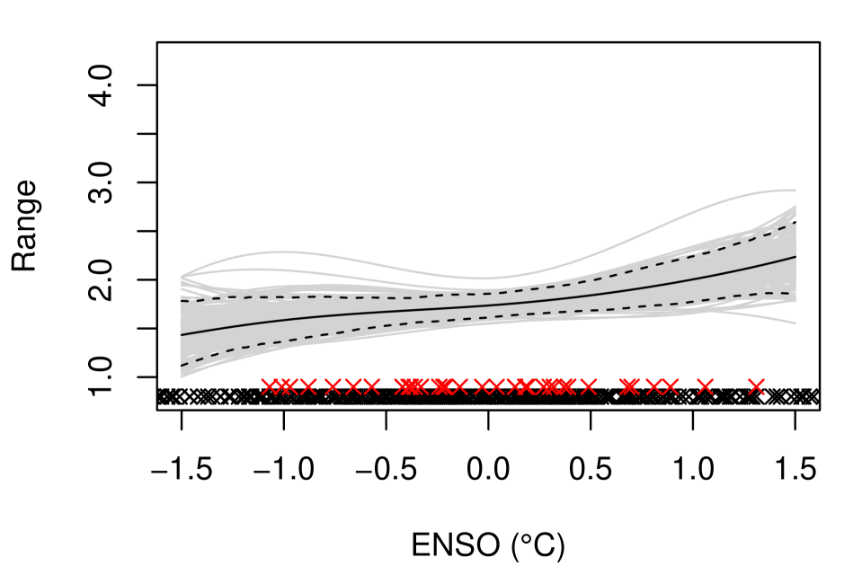
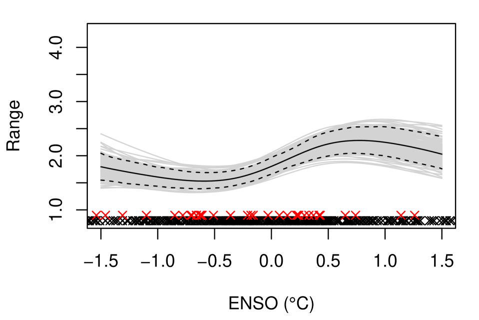
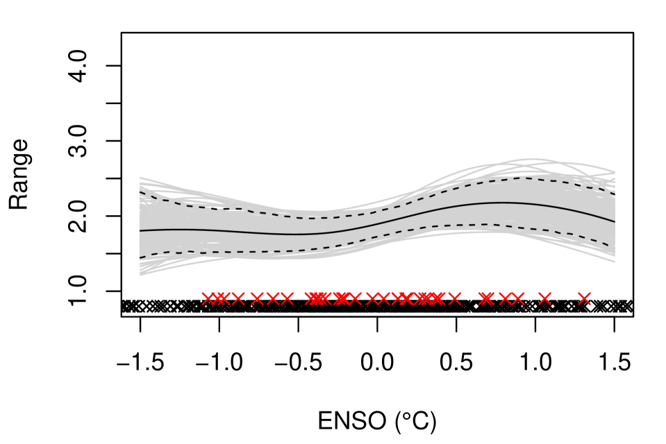
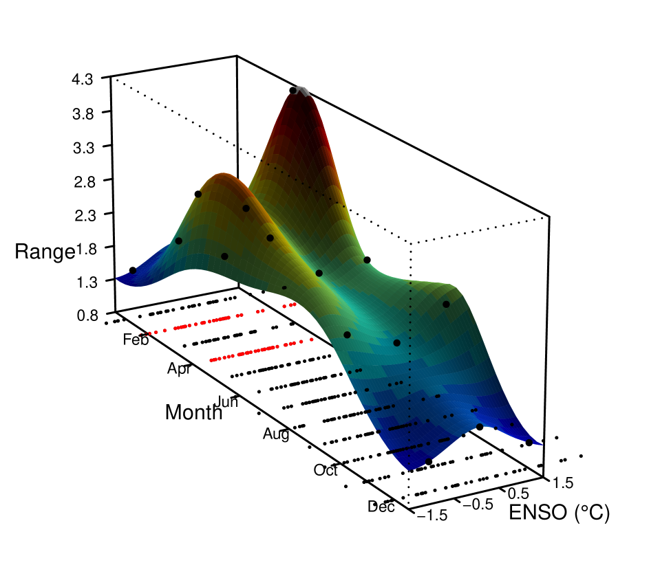
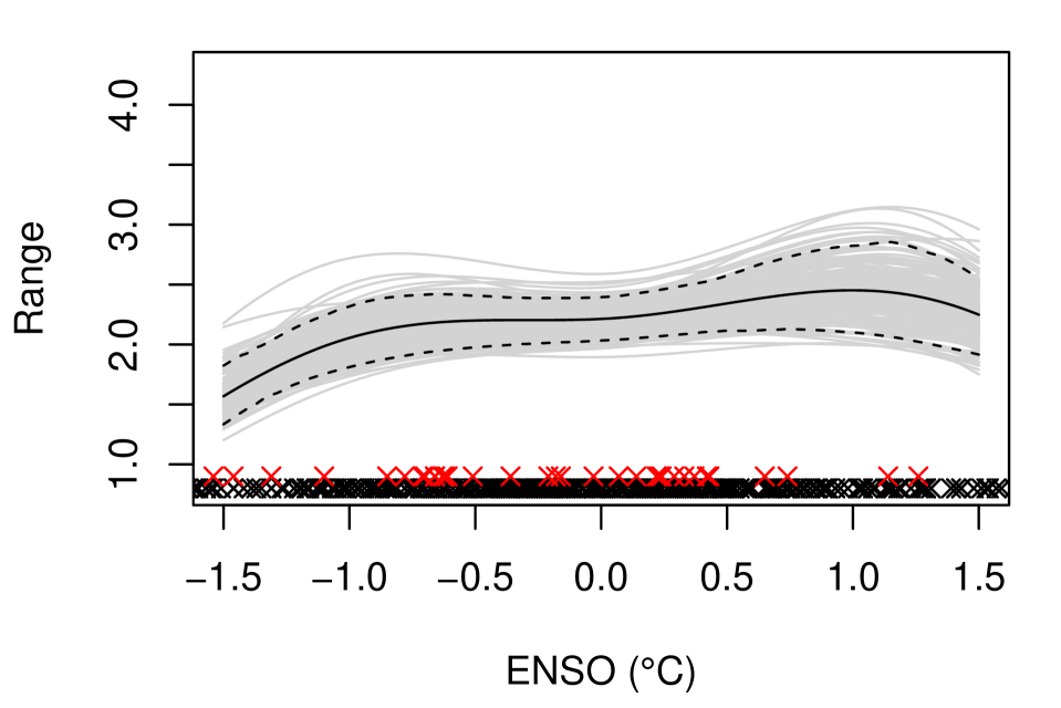
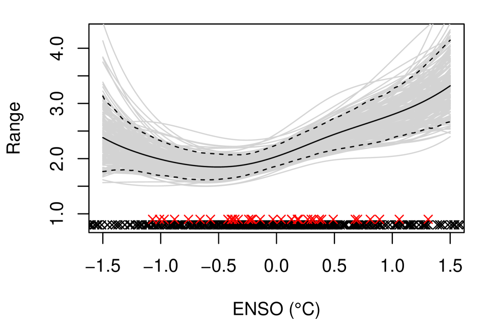
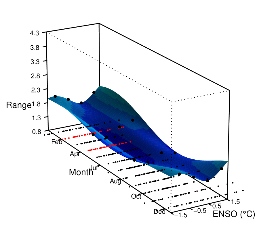
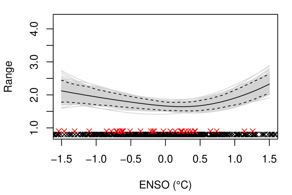
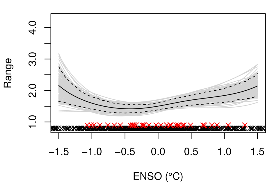
We now discuss the range parameter $\rho$. Figures 4, 5 and 6 show that in nearly all regions $\rho$ is lowest for all variables in July–September and highest in December–May. An exception is CAPE in R3, where the lowest $\rho$ is observed in winter; this is unexpected but has no practical implications because CAPE is rather low over that region in winter.

The variation of $\rho$ with ENSO is more complex. The main effects occur in late winter and spring so, unless otherwise stated, the statements in this paragraph concern these periods. For PROD, in R3, high absolute values of ENSO are associated with much higher values of $\rho$, the clearest signal being during EN. In R4, increased ENSO is linked to an increase in $\rho$, whereas nothing significant is seen for R1 and R2. Regarding CAPE, in R1, high absolute values of ENSO are associated with larger values of $\rho$, the signal being much stronger during LN. Over R2, a slight increase of $\rho$ is noted in winter during EN periods. In R3, large absolute values of ENSO are associated with substantially increased $\rho$, and this effect is even more pronounced during EN. The same is seen in R4, but rather for winter than spring. For SRH, over R1, the range parameter increases slightly with the absolute value of ENSO. In R3, moderate and substantial increases happen during EN and LN, respectively, and similarly for R2, though the effects are more visible in winter. Finally, nothing significant is noted in R4. To summarize, $\rho$ increases during EN and LN (i) for PROD in R3 and R4 (ii) for CAPE in R1, R3 and R4 (iii) for SRH in R1, R2, and R3. Owing to the interpretation of the range $\rho$ in Section 2.1, the seasonal and ENSO-related variations of $\rho$ for the three variables can be interpreted to some degree as variations of the spatial extent of their extremes.

Figure 4: Trend surfaces for the estimated range parameter $\hat{\rho}$ of the model for PROD in Regions 1 (bottom left), 2 (top left), 3 (top right) and 4 (bottom right). The right-hand panels show slices of the surface in February and April (black) with the values of $\exp\{2\log(\hat{\rho})-\log(\hat{\rho}^{\star}_{b})\}$ $(b=1,\dots,200)$ (grey), where $\hat{\rho}^{\star}_{b}$ is the $b$-th bootstrap estimate, and the $90\%$ bootstrap pointwise confidence limits (dashed). On all plots, the rug represents the ENSO values for February and April (red) and other months (black). The larger black dots in the left-hand panels indicate the knots.

Figure 5: Same as in Figure 4, but for CAPE.

Figure 6: Same as in Figure 4, but for SRH.

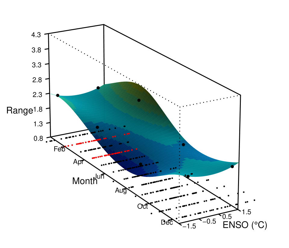
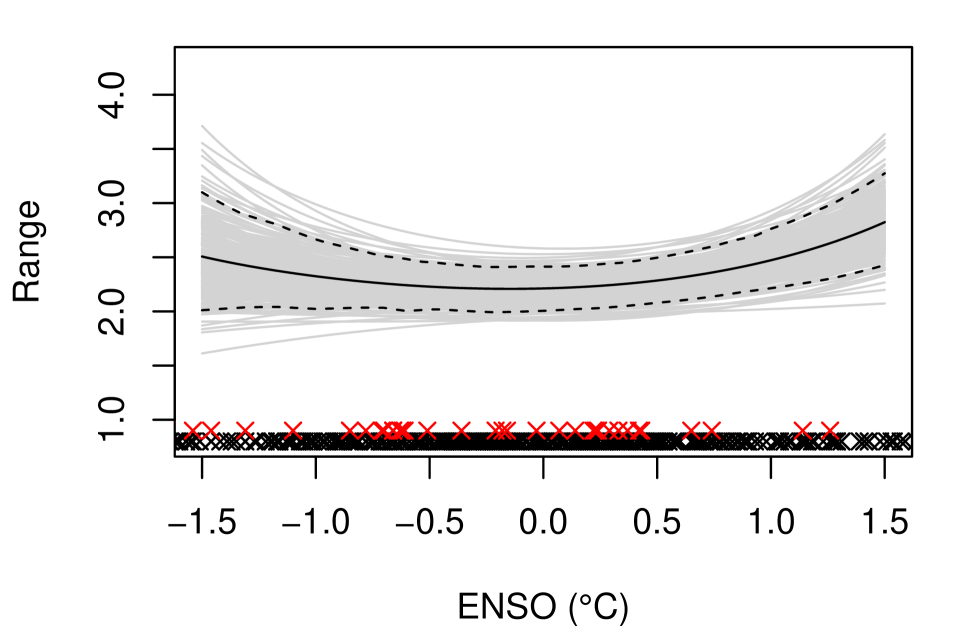
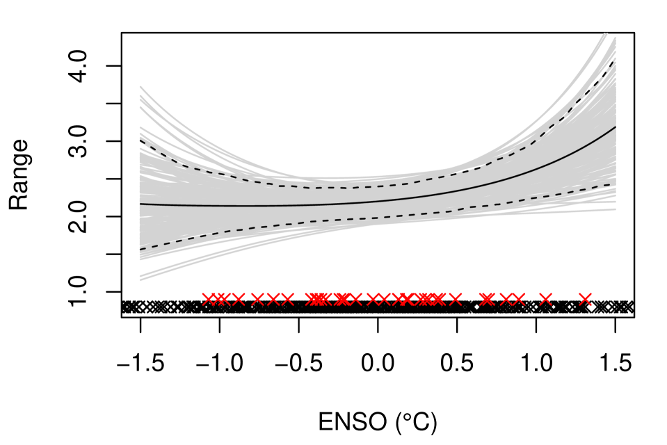
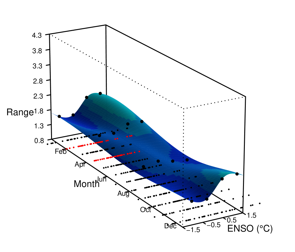
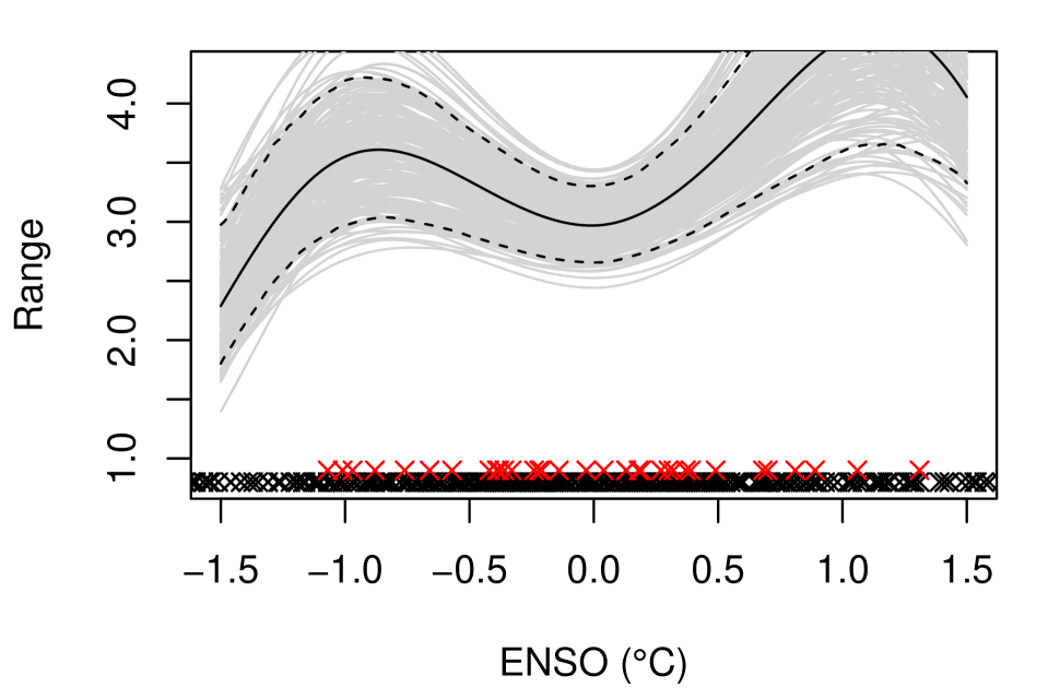
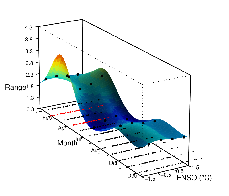
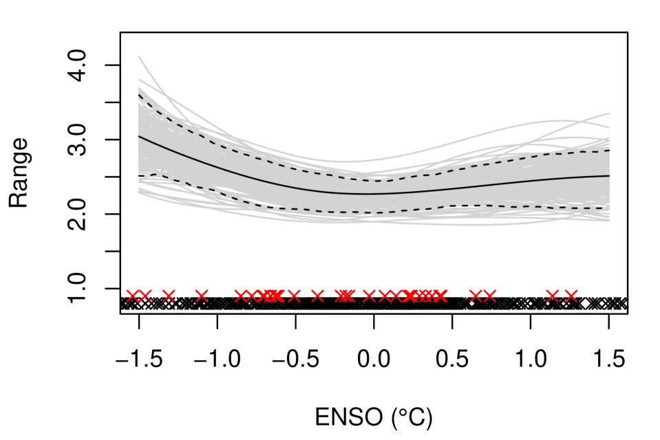
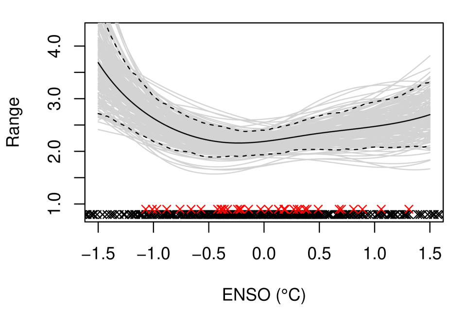
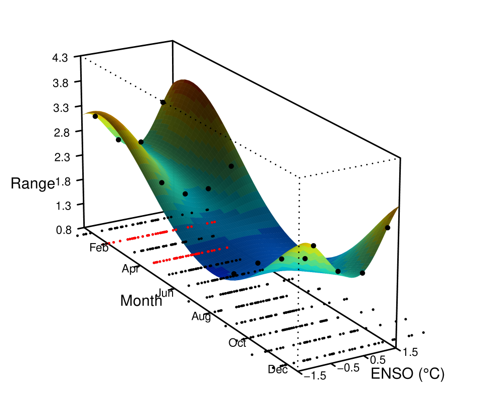
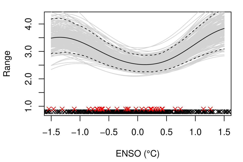
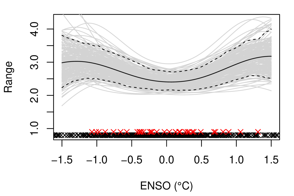
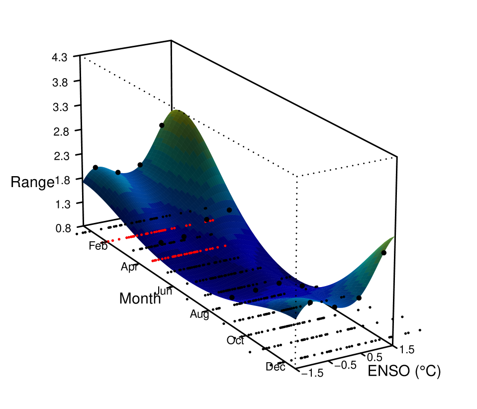
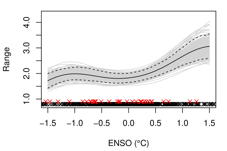
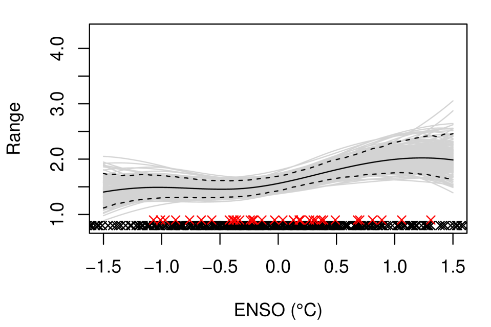
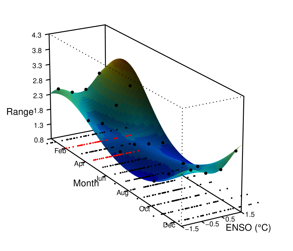
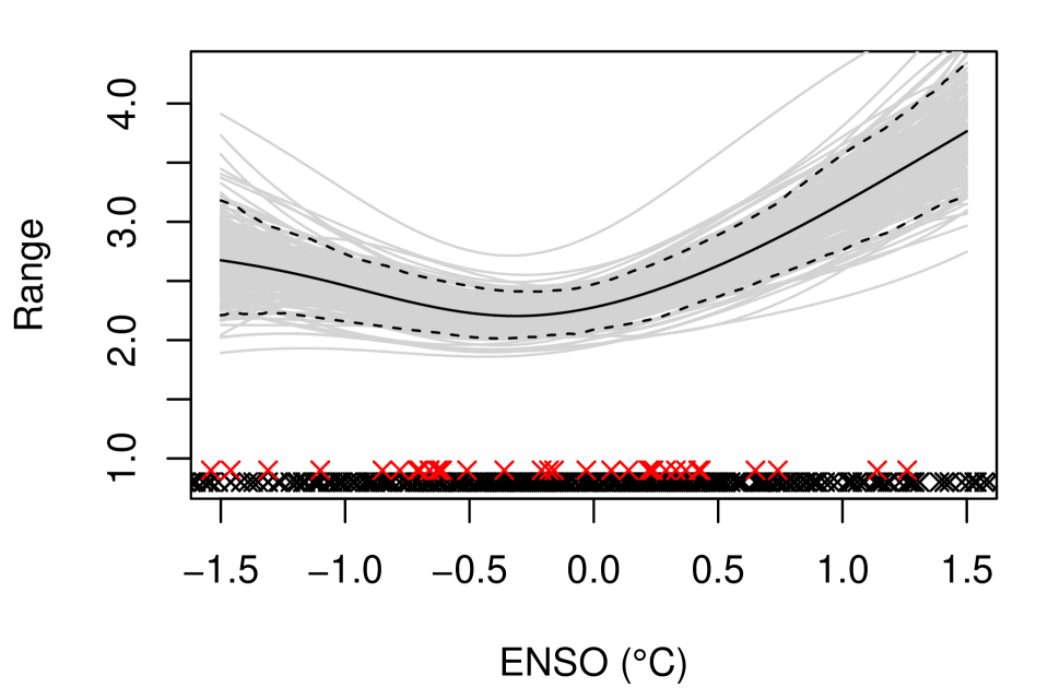
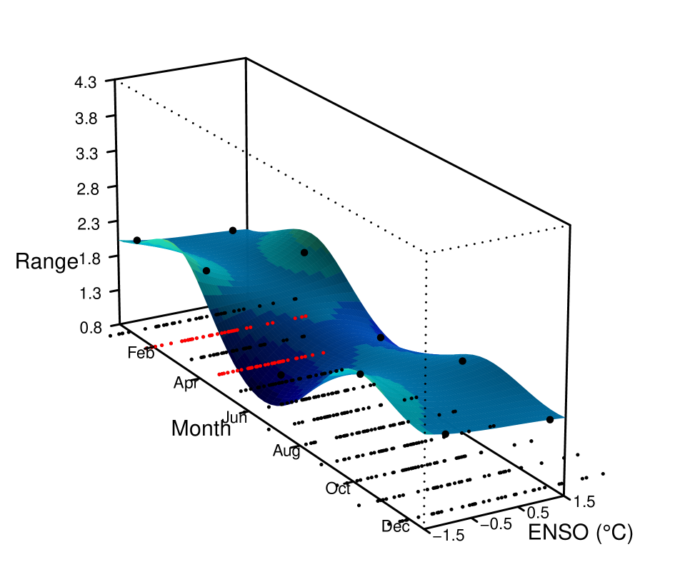
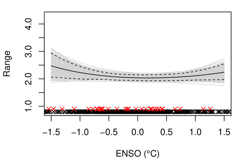
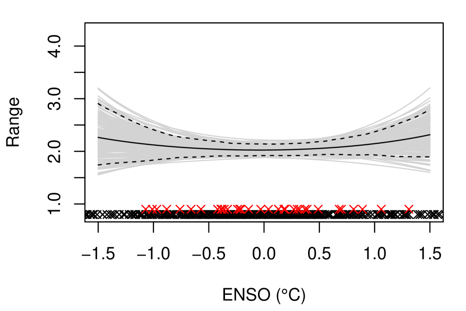
For any value of ENSO and each month, we can compute the bivariate extremal coefficient of our model by combining (7) and (10). Figures 17–19 (Supplementary Material) show the modeled extremal coefficients obtained from the $200$ bootstrap replicates for grid points that are $1^{\circ}$ longitude apart. For $\mathrm{ENSO}=0^{\circ}$C, the estimates are rather stable across months, though they are generally higher in summer. The seasonal variation is more pronounced when $\mathrm{ENSO}=-1^{\circ}$C and $\mathrm{ENSO}=1^{\circ}$C, especially for PROD in R3–4, CAPE in R1, R3–4, and SRH in R1–3. E.g., for SRH in these regions, the estimated extremal coefficient during EN and LN events in July is appreciably higher than in November–April. There is a clear decrease of the extremal coefficient (related to an increase of the range parameter) in late winter and spring during EN years. Finally, we highlight that, owing to the large compression in the longitude direction, the values of modeled extremal coefficients for PROD and SRH in R3 are not in contradiction with those of Figure 1.

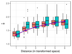
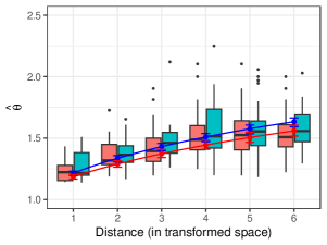
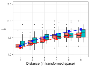
We assessed our model’s performance on the validation set. Figure 7 shows that the theoretical pairwise extremal coefficients computed from our model agree with the empirical ones, despite slight underestimation in the left panel but overestimation in the right. For CAPE and SRH in the chosen region-month combinations, higher values of ENSO are associated with lower empirical extremal coefficients than when ENSO $\approx 0^{\circ}$C, which is not the case for PROD in the chosen region in August; our model captures these effects, and has satisfactory overall out-sample performance.

The few departures between our model and the data probably stem from the spatially-constant extremal dependence in our model within each region although some spatial heterogeneity remains in each case. The fact that the models’ extremal coefficient is computed for particular values of distance and ENSO, whereas the boxplots of Figure 7 are built using a range of distances and ENSO values, may also contribute to the departures.

Figure 7: Out-sample performance of the models for PROD (left), CAPE (center) and SRH (right) for the region-month combinations ($2$-August), ($4$-January) and ($2$-January), respectively. The lines depict the modeled extremal coefficients computed at ENSO=$1^{\circ}$C (red) and $0^{\circ}$C (blue) with respect to distance in the transformed space, computed using (4) with the estimated $\kappa$ and $r$. The whiskers indicate pointwise basic bootstrap $90\%$ confidence limits. The four pairs of boxplots summarize the empirical estimates of the extremal coefficient for pairs of grid points whose distance in the transformed space lies in the ranges $[0.5,1.5)$, $[1.5,2.5)$, $[2.5,3.5)$ and $[3.5,4.5)$. The red and blue boxes correspond to ENSO$\geq 0.5^{\circ}$C and $|\text{ENSO}|<0.5^{\circ}$C, respectively.

4.3 Meteorological interpretation and implications

Extremes of PROD, CAPE and SRH are generally more localized in summer than in winter because lower baroclinicity leads to weaker jet stream-related circulation and thus to a greater importance of local processes and feedbacks.

ENSO is known to modulate the mean latitudinal position of the subtropical jet stream across North America (e.g., Cook and Schaefer, 2008). During the EN phase, the associated changes in the tropics (especially in terms of convection) trigger a southward shift and amplify the subtropical jet stream relative to the N and LN phases. This has direct implications for SRH, as the highest values of vertical shear are typically encountered on the jet stream’s path. R2 and R3 are partially on that path during the N and LN states, but during the EN phase it is much further south; see Figures 4–6 in Cook and Schaefer (2008). During EN, we thus expect lower SRH values for these regions, consistently with what was obtained by Koch et al. (2021), but larger homogeneous spatial patterns compared to N and LN states. During the latter states, some portions of R2 and R3 are on the jet path and some are not, leading to smaller patterns than if the jet was present or absent throughout each region. This accords with the higher range parameter during EN reported for R2 and R3 in Section 4.2; see Figure 6. As shown by Figures 4–6 of Cook and Schaefer (2008), for all ENSO states (LN, N and EN), some pieces of R1 and R4 lie on the jet path and some lie outside. Thus, the size of homogeneous spatial patterns is not expected to vary much with ENSO, consistent with our findings in Section 4.2 (see Figure 7). The meteorological mechanisms linking ENSO and the spatial extent of CAPE events are less explicit than for SRH, since high CAPE values are only indirectly related to the position of the jet. Areas of high CAPE are directly determined by large-scale weather systems such as low-pressure systems and fronts, which themselves are partly driven by the jet stream’s position and intensity. For example, synoptic conditions conducive to advection in the lower troposphere of warm and moist air from the Gulf of Mexico in the presence of rather cold and dry air in the upper troposphere will typically trigger high CAPE. Through their impacts on the jet stream and other potential consequences, variations of ENSO affect the spatial extent of CAPE extremes, but a more detailed meteorological explanation would require deep investigations to shed further light on the very complex physical mechanisms involved. The evolution of the dependence structure of PROD with respect to ENSO inherits from those of CAPE and SRH. The link between ENSO and the spatial extent of weather phenomena has received relatively little attention from researchers; see, e.g., Lyon (2004) and Lyon and Barnston (2005) in the case of the droughts and rainfall extremes.

In spring and summer and when PROD values are high enough for thunderstorms to develop, $\rho$ might be viewed very indirectly as a characteristic dimension of thunderstorm systems (including supercells, multi-cell storms, squall lines, and mesoscale convective complexes). Similarly, if SRH is high enough in winter and spring for cyclones can form, then $\rho$ may be obliquely interpreted as a characteristic dimension of cyclones. But, again, inferring features of cyclonic storms or thunderstorms from conclusions about their proxies must be done with caution. Koch et al. (2021) found that the maxima of PROD, CAPE and SRH tend to be larger during LN in late winter and spring. Combined with this, our findings of Section 4.2 entail that, in spring, thunderstorm systems may be larger in the North-East during LN than the N phase, but the situation for the North-East and South-East during EN remains unclear. Similarly, we cannot draw conclusions about an increase of the extent of cyclonic storms in R2 and R3 (North) during EN, as such a phase is associated with a decrease of SRH values linked to an absence of the jet stream.

5 Discussion

In this paper we propose stochastic models that use covariates such as large-scale atmospheric signals to capture the temporal non-stationarity of the extremal spatial dependence of convective available potential energy (CAPE), storm relative helicity (SRH) and $\mathrm{PROD}=\sqrt{\mathrm{CAPE}}\times\mathrm{SRH}$, variables that are associated with severe US thunderstorms. We use a fractional Brown–Resnick field whose range parameter depends on the El Niño-Southern Oscillation (ENSO) and month to shed light on how these variables affect the spatial extents of these phenomena.

One novel methodological contribution is a max-stability test, based on empirical likelihood and the bootstrap, that accounts for unknown margins and provides a further diagnostic to assess whether a sub-asymptotic model should replace a max-stable model. Another, a bootstrap-based estimator of the composite Kullback–Leibler divergence, enables better model selection than does the CLIC, especially when one first estimates marginal distributions and then uses composite likelihood separately to estimate a dependence structure.

Max-stability appears to be an appropriate assumption for our data. Our findings, combined with those of Koch et al. (2021), suggest that, in the North-East and in spring, thunderstorm systems during LN may be more intense and larger than during neutral ENSO states or EN events. Drawing conclusions about cyclones and thunderstorms for other regions is difficult as translating our findings on their proxies requires caution. Moreover, the reliability of our conclusions depends heavily on the quality of the reanalysis data, in which vertical wind shear (and thus SRH) is typically well-represented, but thermodynamic variables like CAPE are less reliable (see Taszarek et al., 2021, and references therein).

Our model accounts for variation of extremal dependence across time but not over space, a drawback for regions with heterogeneous weather influences. We partially overcome this by applying our model to regions that are rather homogeneous in terms of climate and weather drivers. Allowing smooth spatial variation in the dependence structure, such as in Huser and Genton (2016) or Zhong et al. (2022), could be useful, especially in applications where we are agnostic about the different climatic regions of the domain considered. A local likelihood approach such as that of Hector and Reich (2022) could be used for the fitting. Studying the effects of other atmospheric signals, such as the North Atlantic Oscillation and the Madden–Julian Oscillation, would also be worthwhile, but would require adequate data. Finally, introducing time as a covariate could be beneficial to detect climate-change related influences “orthogonal” to those of the atmospheric signals included in the model.

Using our model for risk assessment or forecasting would require simulated vectors of covariates $\bm{x}_{t}$ ($t=1,\ldots,T$), entailing treating them as realizations of random vectors $\bm{X}_{t}$. Point 2 in the definition of our general model in Section 3.1.1 would then be: the spatial fields $\{Z(\bm{s},1):\bm{s}\in\mathcal{X}\},\ldots,\{Z(\bm{s},T):\bm{s}\in\mathcal{X}\}$ are independent conditionally on $\bm{X}_{1},\ldots,\bm{X}_{T}$. Unconditionally, any temporal dependence would be driven by the dynamics of the random process $\{\bm{X}_{t}:t=1,\ldots,T\}$, but without specific assumptions on that dynamics, the resulting space-time model $\{Z(\bm{s},t):\bm{s}\in\mathcal{X},t=1,\ldots,T\}$ will not be a space-time max-stable field, unlike models developed by Davis et al. (2013), Huser and Davison (2014) or Embrechts et al. (2016).

SUPPLEMENTARY MATERIAL

6 Supplement

6.1 Estimation of max-stable fields

The $D$-dimensional multivariate density of a max-stable random field can be intractable, as the exponent measure in (5) can be difficult to characterize unless $D$ is small and the exponential leads to a combinatorial explosion of the number of terms in the density. Full likelihood inference is thus out of reach in many cases and so composite likelihood techniques (e.g., Varin et al., 2011) have been extensively used. Pairwise composite likelihoods are most common (e.g., Padoan et al., 2010; Blanchet and Davison, 2011; Davison et al., 2012), but higher order composite likelihoods have also been considered (e.g., Huser and Davison, 2013; Castruccio et al., 2016). Under mild regularity conditions, the maximum pairwise likelihood estimator is strongly consistent and asymptotically normal but it has a larger variance than the maximum likelihood estimator. Padoan et al. (2010) and Sang and Genton (2014) showed that truncating the pairwise likelihood by ignoring pairs of sites that are far apart can improve its statistical efficiency; for similar findings in other settings, see the references in Sang and Genton (2014). Ignoring some pairs also decreases the computational burden, which is valuable for large values of $D$, such as our $D=619$. Castruccio et al. (2016) showed that truncation increases statistical efficiency by more for pairwise or triplewise likelihoods than for higher order composite likelihoods.

Let $z_{\bm{s},t}$ denote the maximum at $\bm{s}$ during the $t$-th period, transformed marginally to standard Fréchet, let $\bm{\psi}$ denote the vector of dependence parameters of the max-stable model, and let $f_{\bm{s}_{d},\bm{s}_{d^{\prime}};\bm{\psi}}$ denote the corresponding pairwise density for grid points $\bm{s}_{d},\bm{s}_{d^{\prime}}\in\mathcal{X}$. The truncated pairwise log-likelihood is

$$l(\bm{\psi})=\sum_{t=1}^{T}\sum_{d=1}^{D-1}\sum_{d^{\prime}=d+1}^{D}\mathbb{I}_{\left\{||\bm{s}_{d}-\bm{s}_{d^{\prime}}||\leq\sqrt{2c^{2}}\right\}}\log f_{\bm{s}_{d},\bm{s}_{d^{\prime}};\bm{\psi}}(z_{\bm{s}_{d},t},z_{\bm{s}_{d^{\prime}},t}),$$ (17)

where $c$ is the truncation parameter and $\mathbb{I}_{\{\cdot\}}$ is the indicator function. Choosing truncation distance $\sqrt{2c^{2}}$ rather than $c$ allows us to take all first adjacent neighbors into account, including those on the diagonals.

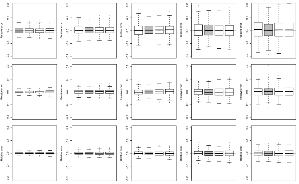
We chose a value of $c$ adapted to the present context by simulating Brown–Resnick fields having semivariogram (3) with $r=1$, $\kappa=0$, $\alpha=1$ and $\rho\in\{1,2,4,8,12\}$, on squares containing $25$, $100$, and $225$ grid points. In each of these $15$ settings, we simulated $444$ (the number of months in our data) independent realizations of the field $400$ times independently. For each of these $400$ experiments, we estimated $\rho$ using the truncated pairwise log-likelihood (17) with $c\in\{1,2,3,4\}$. The smoothness parameter $\alpha=1$ and scaling and rotation parameters $r=1$ and $\kappa=0$ are close to the estimates from our data. We let the range $\rho$ and the spatial domain vary, as the optimal truncation distance depends on both. Our results (Figure 8) show that estimation becomes more precise when $\rho$ decreases and $D$ increases. In most settings $c=2$ leads to more precise estimation, and we use this value for our case study.

Figure 8: Boxplots of the relative errors of the estimates of $\rho$ for $c=1,2,3,4$ (from left to right). The boxplot associated with the lowest relative root mean squared error is highlighted in grey. The rows correspond to $D=25$ (top), $100$ (middle), $225$ (bottom) and each column corresponds to a value of $\rho$: $1,2,4,8,12$ (from left to right).

6.2 Simulation study for Section 3.1.2

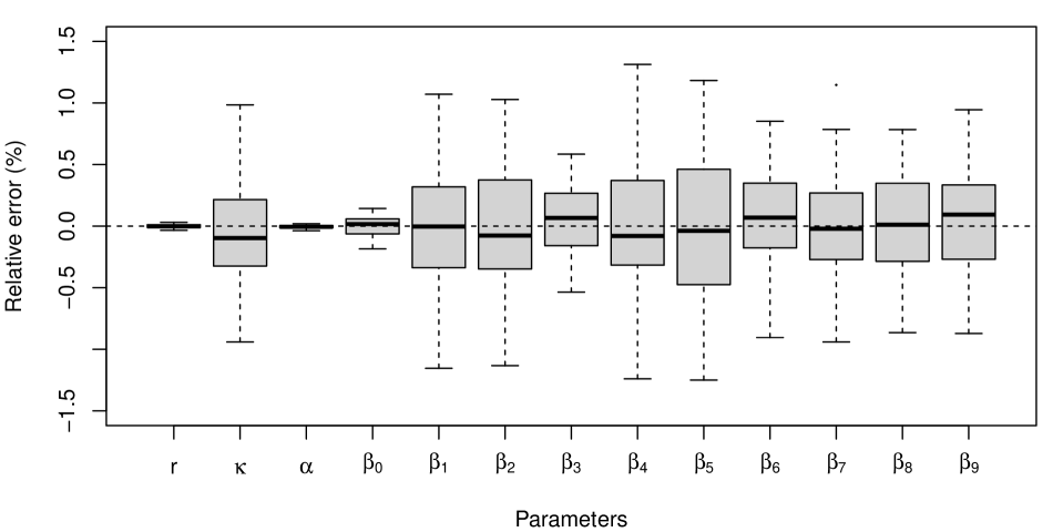
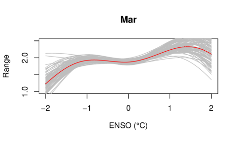
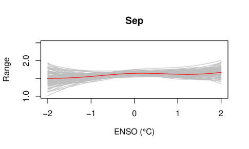
We consider (10) with $T=444$ on a square containing 100 grid points, corresponding to the lowest number of grid points considered in our case study, and with parameters $r=0.72$, $\kappa=-0.08$, and $\alpha=1.26$, three knots with coordinates $-1.06$, $0.05$, $1.16$ in the ENSO direction, and knots at $0.5$, $4.5$, $8.5$, $12.5$ in the month direction. As we use a circular P spline basis for months, the values of the spline are the same at $0.5$ and $12.5$, giving three distinct knots in both the ENSO and month directions, i.e., nine knots over the space of covariates. The corresponding coefficients, $\beta_{0}=0.52$ (intercept), $\beta_{1}=-0.03$, $\beta_{2}=0.02$, $\beta_{3}=0.07$, $\beta_{4}=0.11$, $\beta_{5}=-0.07$, $\beta_{6}=-0.23$, $\beta_{7}=-0.03$, $\beta_{8}=0.02$ and $\beta_{9}=0.04$, correspond to those obtained when fitting this model to the data described in Section 2.2. We estimate all the parameters for $100$ independent replicates of such data. Figure 9 suggests that all the estimators are essentially unbiased and that all parameters are recovered well, but that the estimators of the parameters associated with the spline basis tend to more variable than are the others. The smoothness parameter $\alpha$ and the scaling factor $r$ are very well estimated. Figure 10 also shows that signals and non-signals are equally well-identified.

Figure 9: Relative error for the parameters in the simulation study.

Figure 10: The estimated range parameter with form given in (9), based on the same simulation study as that in Figure 9, for $t$ mod $12$ = 3 (March, left) and $t$ mod $12$ = 9 (September, right).

6.3 For Section 3.2

6.3.1 Algorithms

Let $\bm{{y}}_{j}=({y}_{1,j},\dots,{y}_{D,j})^{\prime}$ denote the $j$-th underlying (here, three-hourly) observation, empirically transformed to be standard Fréchet-distributed, where $D$ is the number of grid points. Given $n_{M}$ underlying (here again, three-hourly) observations over all years, i.e., $n_{M}=n$ (block size) $\times M$ (number of years), let $({\bm{y}_{1}},\dots,{\bm{y}_{n_{M}}})^{\prime}\in\mathbb{R}^{n_{M}\times D}$ denote the transformed dataset. The procedure for generating the max-stable vector is

1. Compute $\tilde{R}_{j}=||y_{1,j},\dots,y_{D,j}||_{1}$, known as the radial coordinates, where $||\cdot||_{1}$ is the $L_{1}$ norm. Then calculate $\bm{\tilde{W}_{j}}=\bm{y}_{j}/\tilde{R}_{j}$, $j=1,\dots,n_{M}$, commonly called the angular coordinates. Keep those $\bm{\tilde{W}}_{j}$ for which $\tilde{R}_{j}>r_{0}$, with $r_{0}$ fixed to be the empirical $p$-quantile of $\tilde{R}_{1},\dots,\tilde{R}_{n}$, so the number of observations retained is $n_{0}=(1-p)n_{M}$, where $0<p<1$. Let $R_{i}$ and $\bm{W}_{i}$ ($i=1,\dots,n_{0}$) denote the coordinates retained.

2. Following the empirical likelihood approach of Einmahl and Segers (2009), but extended to $D>2$, we find the estimated angular probability measure

   $$\hat{Q}(\bm{w})=\sum_{i=1}^{n_{0}}q_{i}\mathbb{I}_{\{\bm{W}_{i}<\bm{w}\}},\quad\bm{w}\in[0,1]^{D},$$

   where $\mathbb{I}_{\{\cdot\}}$ is the indicator function and the tilting probabilities $\{q_{i}\}_{i=1}^{n_{0}}$ satisfy

   $$q_{i}=\operatorname*{arg\,max}_{q_{i}}\prod_{i=1}^{n_{0}}q_{i},\text{ such that }\sum_{i=1}^{n_{0}}q_{i}=1\text{ and }\sum_{i}^{n_{0}}q_{i}\bm{W}_{i}/R_{i}=\bm{D}^{-1},$$ (18)

   where $\bm{D}^{-1}=(1/D,\dots,1/D)^{\prime}$, and (18) is solved using Lagrange multipliers.

3. With $\{q_{i}\}_{i=1}^{n_{0}}$ and $\{\bm{W}_{i}\}_{i=1}^{n_{0}}$, generate a simple max-stable vector using Algorithm 1, based on Dombry et al. (2016).

Input: Tilting weights $\{q_{i}\}_{i=1}^{n_{0}}$ and vectors $\{\bm{W}_{i}\}_{i=1}^{n_{0}}$

Output: Max-stable $D$-dimensional vector with standard Frechét margins

Generate $E^{\star}\sim\text{Exp}(1)$ ;

Set $R^{\star}=D/E^{\star}$;

Set $\bm{Z}=(Z_{1},\dots,Z_{D})=(0,\dots,0)$;

while $R^{\star}>\min\{Z_{1},\dots,Z_{D}\}$ do

       Draw $\bm{W}^{{}^{\prime}}=(W_{1}^{{}^{\prime}},\dots,W_{D}^{{}^{\prime}})$ from the set $\{\bm{W}_{1},\dots,\bm{W}_{n_{0}}\}$ with sampling probabilities $\{q_{1},\dots,q_{n_{0}}\}$;

       for $j\leftarrow 1$ to $D$ do

             Set $Z_{j}=\max(Z_{j},R^{\star}W_{j}^{{}^{\prime}})$;

            

       end for

      Generate $E^{\star}\sim\text{Exp}(1)$;

       Set $R^{\star}=\frac{1}{(1/R^{\star}+E^{\star}/D)}$;

      

end while

return $\bm{Z}$ ;

Algorithm 1 Simulate max-stable vector using tilting weights

6.3.2 Simulation study

We first generate from a multivariate logistic extreme-value distribution

$$G(y_{1},\ldots,y_{D})=\exp\left\{-\left(\sum_{d=1}^{D}y_{d}^{-1/\lambda}\right)^{\lambda}\right\},\quad y_{1},\ldots,y_{D}>0,$$

with dependence parameter $\lambda\in\{0.1,0.5,0.9\}$, and perform our max-stability test on these observations with $B=200$. We then repeat this experiment with data from a multivariate Gaussian distribution with common pairwise correlation $\zeta\in\{0.1,0.5,0.9,0.99\}$. To assess the empirical size and power of the test, we replicate both experiments $500$ times. Pointwise maxima of Gaussian fields converge in (1) to the degenerate independent max-stable field, but a block size of $240$ is insufficient for convergence, so using the multivariate normal distribution is an approximate but reasonable way to assess the power of our test.

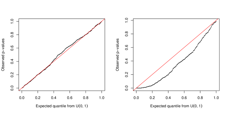
Table 3 shows that the empirical size of the test is controlled reasonably well in this setting, with the 500 A-D and Kolmogorov–Smirnov p-values correctly showing no departure from uniformity at the $5\%$ level for the logistic models, which are max-stable. Uniformity of the p-values for the multivariate normal model is rejected at the $5\%$ level except when $\zeta=0.1$, perhaps because the block maxima are already close to the independent max-stable distribution as this convergence becomes quicker with decreasing $\zeta$. As expected, the power rises as dependence increases. Figure 11, which shows quantile-quantile plots of the p-values in two simulation settings, illustrates the departure from uniformity in the Gaussian case.

	$5\%$	$20\%$	p-val AD	p-val KS
Max-stable logistic, $\lambda=0.1$	5.40	18.80	0.20	0.18
Max-stable logistic, $\lambda=0.5$	4.80	19.00	0.71	0.83
Max-stable logistic, $\lambda=0.9$	5.40	20.00	0.40	0.22
Normal, $\zeta=0.1$	4.80	21.40	0.48	0.65
Normal, $\zeta=0.5$	14.20	31.40	0.00	0.00
Normal, $\zeta=0.9$	22.00	40.40	0.00	0.00

Table 3: Empirical size $(\%)$ (top three) and power $(\%)$ (bottom three) for tests at the $5\%$ and $20\%$ nominal level with $(B,p)=(200,0.9)$, for $500$ samples of size $n_{M}=240\times 40$, and different levels of dependence. The last two columns show the p-values for the Anderson–Darling and Kolmogorov–Smirnoff tests of uniformity for the 500 p-values.

Figure 11: Quantile-quantile plots for the $500$ p-values with the simulation setting involving the max-stable logistic, $\lambda=0.1$ (left), and normal, ${\color[rgb]{0,0,0}\zeta}=0.9$ (right), distributions.

6.4 For Section 3.3

Figure 12: Nominal $95\%$ sandwich (left) and bootstrap (right) confidence intervals for the range parameter $\rho$ (with logarithm as variance-stabilizing transform) in the model BR₁ using the two-step estimation procedure, from 200 simulations with 40 replications, $D=25$ (top) and $D=225$ (bottom). The red confidence intervals represent those that do not cover the true value represented by the red dashed line.

6.5 For Section 4.1

Figure 13 shows the resulting clusters from applying the PAM to chosen monthly maxima.

Figure 13: Resulting clusters (indicated with different colours) from applying the algorithm of Bernard et al. (2013) with four clusters on our July maxima for PROD (left), CAPE (centre) and SRH (right).

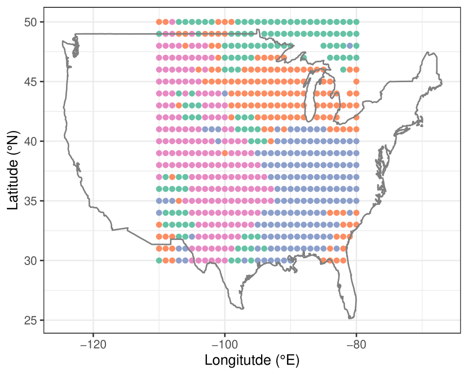
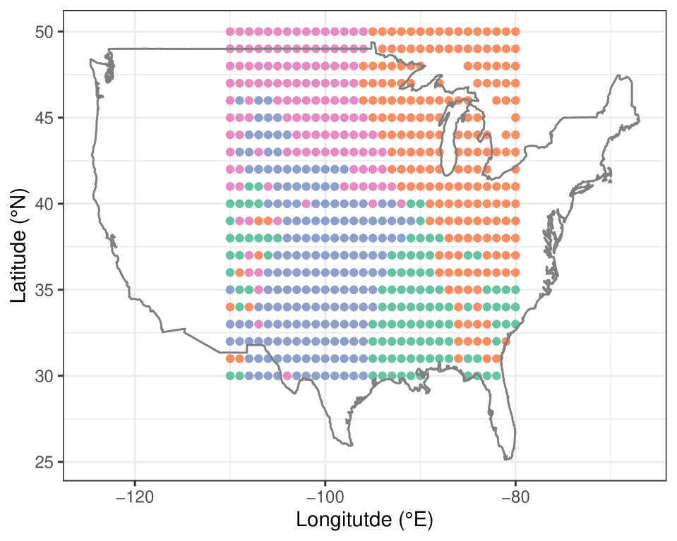
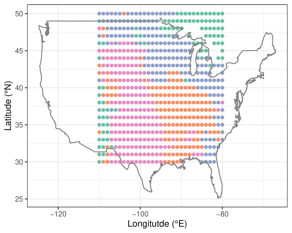
Figure 14 shows the p-values from applying our max-stability test to the data.

Figure 14: P-values from applying our max-stability test on the region (in numbers from 1-4) month (x-axes) combinations for PROD (left), CAPE (centre) and SRH (right). The dashed horizontal lines indicate the 0.05 level.

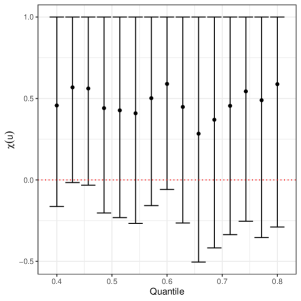
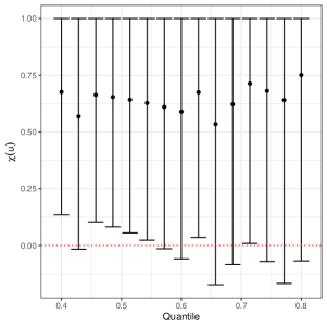
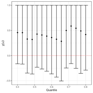
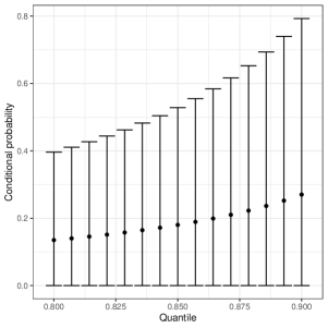
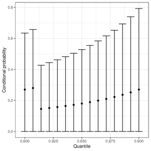
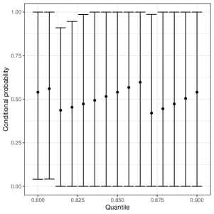
Here we describe the two types of diagnostic plots implemented in our case study. For two random variables $X_{1}$ and $X_{2}$ with bivariate distribution function $F$ and marginal distribution functions $F_{1}$ and $F_{2}$, two measures of dependence are

$$\chi(u)=2-\frac{\log\Pr(F_{1}(X_{1})<u,F_{2}(X_{2})<u)}{\log\Pr(F_{2}(X_{2})<u)},\quad 0\leq u\leq 1.$$

and

$$\chi^{\prime}(u)=\mathrm{Pr}\{F_{1}(X_{1})>u\mid F_{2}(X_{2})>u\}.$$

It is straightforward to see that $\lim_{u\to 1}\chi(u)=\lim_{u\to 1}\chi^{\prime}(u).$ If $F$ is a bivariate max-stable distribution, then $\chi^{\prime}(u)$ stabilises as $u\rightarrow 1$, and $\chi(u)$ is stable for all $u\in[0,1]$ (Coles et al., 1999). In practice, due to the lack of data when $u$ is close to 0 and 1, the two measures are only evaluated in the regions between the two values.

Figure 15 finds no evidence that $\chi(u)$ is unstable for randomly chosen locations for all variables. There is also no evidence that $\chi^{\prime}(u)$ is weakening for increasingly high thresholds, though both plots are associated with high confidence intervals.

Figure 15: Empirical estimates of $\chi(u)$ for $u\in[0.2,0.8]$, for the monthly maxima from two random locations in region-variable (left to right): 2-PROD, 4-CAPE and 1-SRH

Figure 16: Empirical estimates of $\chi^{\prime}(u)$ for $u\in[0.8,0.9]$, for the monthly maxima from two random locations in region-variable (left to right): 1-PROD, 3-CAPE and 2-SRH

6.6 For Section 4.2

Figures 17, 18 and 19 shows the modeled bivariate extremal coefficient estimates obtained from $200$ bootstrap replicates for grid points that are $1^{\circ}$ longitude apart.

Figure 17: Bias-corrected estimates (blue) of the modeled bivariate extremal coefficient for PROD in regions 1 (bottom left), 2 (top left), 3 (top right) and 4 (bottom right), when ENSO equals $-1^{\circ}$C (left), $0^{\circ}$C (center) and $1^{\circ}$C (right), for two grid points $1^{\circ}$ longitude apart. The grey dots are the $200$ values of $h^{-1}\{2h(\hat{\theta})-h(\hat{\theta}^{\star}_{b})\}$, $b=1,\dots,200$, where $\hat{\theta}^{\star}_{b}$ is the $b$-th bootstrap estimate and $h(x)=\log\{(x-1)/(2-x)\}$, for $x\in[1,2]$. The black dots indicate the lower and upper $90\%$ bootstrap pointwise confidence limits.

Figure 18: Same as Figure 17 but for CAPE.

Figure 19: Same as Figure 17 but for SRH.

References

- (1)
- Allen and Tippett (2015) Allen, J. T. and Tippett, M. K. (2015), ‘The characteristics of United States hail reports: 1955-2014’, Electronic Journal of Severe Storms Meteorology 10(3), 1–31.
- Allen et al. (2015) Allen, J. T., Tippett, M. K. and Sobel, A. H. (2015), ‘Influence of the El Niño/Southern Oscillation on tornado and hail frequency in the United States’, Nature Geoscience 8, 278–283.
- Anderson and Darling (1954) Anderson, T. W. and Darling, D. A. (1954), ‘A test of goodness of fit’, Journal of the American Statistical Association 49, 765–769.
- Bacro et al. (2010) Bacro, J.-N., Bel, L. and Lantuéjoul, C. (2010), ‘Testing the independence of maxima: from bivariate vectors to spatial extreme fields’, Extremes 13, 155–175.
- Beck et al. (2018) Beck, H. E., Zimmermann, N. E., McVicar, T. R., Vergopolan, N., Berg, A. and Wood, E. F. (2018), ‘Present and future Köppen–Geiger climate classification maps at 1-km resolution’, Scientific Data 5, 180214.
- Bernard et al. (2013) Bernard, E., Naveau, P., Vrac, M. and Mestre, O. (2013), ‘Clustering of maxima: Spatial dependencies among heavy rainfall in france’, Journal of Climate 26(20), 7929–7937.
- Blanchet and Davison (2011) Blanchet, J. and Davison, A. C. (2011), ‘Spatial modeling of extreme snow depth’, Annals of Applied Statistics 5(3), 1699–1725.
- Brooks (2013) Brooks, H. E. (2013), ‘Severe thunderstorms and climate change’, Atmospheric Research 123, 129–138.
- Brooks et al. (2003) Brooks, H. E., Lee, J. W. and Craven, J. P. (2003), ‘The spatial distribution of severe thunderstorm and tornado environments from global reanalysis data’, Atmospheric Research 67–68, 73–94.
- Brown and Resnick (1977) Brown, B. M. and Resnick, S. I. (1977), ‘Extreme values of independent stochastic processes’, Journal of Applied Probability 14(4), 732–739.
- Buhl and Klüppelberg (2016) Buhl, S. and Klüppelberg, C. (2016), ‘Anisotropic Brown–Resnick space-time processes: estimation and model assessment’, Extremes 19(4), 627–660.
- Castruccio et al. (2016) Castruccio, S., Huser, R. and Genton, M. G. (2016), ‘High-order composite likelihood inference for max-stable distributions and processes’, Journal of Computational and Graphical Statistics 25(4), 1212–1229.
- Cavanaugh and Shumway (1997) Cavanaugh, J. E. and Shumway, R. H. (1997), ‘A bootstrap variant of AIC for state-space model selection’, Statistica Sinica 7(2), 473–496.
- Coles (2001) Coles, S. (2001), An Introduction to Statistical Modeling of Extreme Values, Springer.
- Coles et al. (1999) Coles, S., Heffernan, J. and Tawn, J. (1999), ‘Dependence measures for extreme value analyses’, Extremes 2(4), 339–365.
- Cook and Schaefer (2008) Cook, A. R. and Schaefer, J. T. (2008), ‘The relation of El Niño–Southern Oscillation (ENSO) to winter tornado outbreaks’, Monthly Weather Review 136(8), 3121–3137.
- Cooley et al. (2006) Cooley, D., Naveau, P. and Poncet, P. (2006), Variograms for spatial max-stable random fields, in P. Bertail, P. Soulier and P. Doukhan, eds, ‘Dependence in Probability and Statistics’, Springer, New York, pp. 373–390.
- Davis et al. (2013) Davis, R. A., Klüppelberg, C. and Steinkohl, C. (2013), ‘Max-stable processes for modeling extremes observed in space and time’, Journal of the Korean Statistical Society 42(3), 399–414.
- Davison and Hinkley (1997) Davison, A. C. and Hinkley, D. V. (1997), Bootstrap Methods and their Application, Cambridge University Press.
- Davison et al. (2013) Davison, A. C., Huser, R. and Thibaud, E. (2013), ‘Geostatistics of dependent and asymptotically independent extremes’, Mathematical Geosciences 45(5), 511–529.
- Davison et al. (2018) Davison, A. C., Huser, R. and Thibaud, E. (2018), Spatial extremes, in A. E. Gelfand, M. Fuentes, J. A. Hoeting and R. L. Smith., eds, ‘Handbook of Environmental and Ecological Statistics’, CRC Press.
- Davison et al. (2012) Davison, A. C., Padoan, S. A. and Ribatet, M. (2012), ‘Statistical modeling of spatial extremes (with Discussion)’, Statistical Science 27(2), 161–186.
- de Carvalho and Ramos (2012) de Carvalho, M. and Ramos, A. (2012), ‘Bivariate extreme statistics, II’, Revstat-Statistical Journal 10, 81–104.
- de Haan (1984) de Haan, L. (1984), ‘A spectral representation for max-stable processes’, Annals of Probability 12(4), 1194–1204.
- de Haan and Ferreira (2006) de Haan, L. and Ferreira, A. (2006), Extreme Value Theory: An Introduction, Springer.
- Dombry et al. (2016) Dombry, C., Engelke, S. and Oesting, M. (2016), ‘Exact simulation of max-stable processes’, Biometrika 103(2), 303–317.
- Dombry et al. (2018) Dombry, C., Ribatet, M. and Stoev, S. (2018), ‘Probabilities of concurrent extremes’, Journal of the American Statistical Association 113(524), 1565–1582.
- Doswell III (2015) Doswell III, C. A. (2015), Mesoscale meteorology — severe storms, in ‘Encyclopedia of Atmospheric Sciences’, pp. 361–368.
- Edwards et al. (2018) Edwards, R., Allen, J. T. and Carbin, G. W. (2018), ‘Reliability and climatological impacts of convective wind estimations’, Journal of Applied Meteorology and Climatology 57(8), 1825–1845.
- Einmahl and Segers (2009) Einmahl, J. H. J. and Segers, J. J. (2009), ‘Maximum empirical likelihood estimation of the spectral measure of an extreme-value distribution’, Annals of Statistics 37, 2953–2989.
- Embrechts et al. (2016) Embrechts, P., Koch, E. and Robert, C. Y. (2016), ‘Space–time max-stable models with spectral separability’, Advances in Applied Probability 48(A), 77–97.
- Gabda et al. (2012) Gabda, D., Towe, R., Wadsworth, J. and Tawn, J. (2012), ‘Discussion of “Statistical Modelling of Spatial Extremes” by A.C. Davison, S.A. Padoan and M. Ribatet’, Statistical Science 27(2), 189–192.
- Gilleland (2020) Gilleland, E. (2020), ‘Bootstrap methods for statistical inference. Part II: Extreme-value analysis’, Journal of Atmospheric and Oceanic Technology 37(11), 2135–2144.
- Gilleland et al. (2013) Gilleland, E., Brown, B. G. and Ammann, C. M. (2013), ‘Spatial extreme value analysis to project extremes of large-scale indicators for severe weather’, Environmetrics 24, 418–432.
- Heaton et al. (2011) Heaton, M. J., Katzfuss, M., Ramachandar, S., Pedings, K., Gilleland, E., Mannshardt-Shamseldin, E. and Smith, R. L. (2011), ‘Spatio-temporal models for large-scale indicators of extreme weather’, Environmetrics 22(3), 294–303.
- Hector and Reich (2022) Hector, E. C. and Reich, B. J. (2022), ‘Distributed inference for spatial extremes modeling in high dimensions’.
- Heffernan and Tawn (2004) Heffernan, J. E. and Tawn, J. A. (2004), ‘A conditional approach for multivariate extreme values (with discussion)’, Journal of the Royal Statistical Society: Series B (Statistical Methodology) 66(3), 497–546.
- Hoerling et al. (1997) Hoerling, M. P., Kumar, A. and Zhong, M. (1997), ‘El Niño, La Niña, and the nonlinearity of their teleconnections’, Journal of Climate 10(8), 1769–1786.
- Huber (1964) Huber, P. J. (1964), ‘Robust estimation of a location parameter’, Annals of Mathematical Statistics 35, 73–101.
- Huser and Davison (2013) Huser, R. and Davison, A. C. (2013), ‘Composite likelihood estimation for the Brown–Resnick process’, Biometrika 100(2), 511–518.
- Huser and Davison (2014) Huser, R. and Davison, A. C. (2014), ‘Space-time modelling of extreme events’, Journal of the Royal Statistical Society: Series B (Statistical Methodology) 76(2), 439–461.
- Huser and Genton (2016) Huser, R. and Genton, M. G. (2016), ‘Non-stationary dependence structures for spatial extremes’, Journal of Agricultural, Biological, and Environmental Statistics 21, 470–491.
- Huser et al. (2017) Huser, R., Opitz, T. and Thibaud, E. (2017), ‘Bridging asymptotic independence and dependence in spatial extremes using Gaussian scale mixtures’, Spatial Statistics 21, 166–186.
- Huser et al. (2021) Huser, R., Opitz, T. and Thibaud, E. (2021), ‘Max-infinitely divisible models and inference for spatial extremes’, Scandinavian Journal of Statistics 48(1), 321–348.
- Huser and Wadsworth (2019) Huser, R. and Wadsworth, J. L. (2019), ‘Modeling spatial processes with unknown extremal dependence class’, Journal of the American Statistical Association 114(525), 434–444.
- Kabluchko and Schlather (2010) Kabluchko, Z. and Schlather, M. (2010), ‘Ergodic properties of max-infinitely divisible processes’, Stochastic Processes and their Applications 120(3), 281–295.
- Kabluchko et al. (2009) Kabluchko, Z., Schlather, M. and de Haan, L. (2009), ‘Stationary max-stable fields associated to negative definite functions’, Annals of Probability 37(5), 2042–2065.
- Koch et al. (2021) Koch, E., Koh, J., Davison, A. C., Lepore, C. and Tippett, M. K. (2021), ‘Trends in the extremes of environments associated with severe U.S. thunderstorms’, Journal of Climate 34(4), 1259–1272.
- Lepore et al. (2017) Lepore, C., Tippett, M. K. and Allen, J. T. (2017), ‘ENSO-based probabilistic forecasts of March–May US tornado and hail activity’, Geophysical Research Letters 44(17), 9093–9101.
- Lyon (2004) Lyon, B. (2004), ‘The strength of El Niño and the spatial extent of tropical drought’, Geophysical Research Letters 31(21).
- Lyon and Barnston (2005) Lyon, B. and Barnston, A. G. (2005), ‘ENSO and the spatial extent of interannual precipitation extremes in tropical land areas’, Journal of Climate 18(23), 5095–5109.
- Mannshardt and Gilleland (2013) Mannshardt, E. and Gilleland, E. (2013), ‘Extremes of severe storm environments under a changing climate’, American Journal of Climate Change 2(3A), 47–61.
- Markowski and Richardson (2010) Markowski, P. and Richardson, Y. (2010), Mesoscale Meteorology in Midlatitudes, Wiley.
- McNemar (1947) McNemar, Q. (1947), ‘Note on the sampling error of the difference between correlated proportions or percentages’, Psychometrika 12(2), 153–157.
- Mhalla et al. (2017) Mhalla, L., Chavez-Demoulin, V. and Naveau, P. (2017), ‘Non-linear models for extremal dependence’, Journal of Multivariate Analysis 159, 49–66.
- Opitz (2013) Opitz, T. (2013), ‘Extremal processes: elliptical domain of attraction and a spectral representation’, Journal of Multivariate Analysis 122, 409–413.
- Padoan et al. (2010) Padoan, S. A., Ribatet, M. and Sisson, S. A. (2010), ‘Likelihood-based inference for max-stable processes’, Journal of the American Statistical Association 105(489), 263–277.
- Pickands (1981) Pickands, J. (1981), ‘Multivariate extreme value distributions’, Bulletin of the International Statistical Institute: Proceedings of the 43rd Session of the International Statistical Institute, Vol. 2 (Buenos Aires) pp. 859–878, 894–902.
- Sang and Genton (2014) Sang, H. and Genton, M. G. (2014), ‘Tapered composite likelihood for spatial max-stable models’, Spatial Statistics 8, 86–103.
- Schlather (2002) Schlather, M. (2002), ‘Models for stationary max-stable random fields’, Extremes 5, 33–44.
- Schlather and Tawn (2003) Schlather, M. and Tawn, J. A. (2003), ‘A dependence measure for multivariate and spatial extreme values: properties and inference’, Biometrika 90(1), 139–156.
- Shibata (1997) Shibata, R. (1997), ‘Bootstrap estimate of Kullback-Leibler information for model selection’, Statistica Sinica 7, 375–394.
- Smith and Stephenson (2009) Smith, E. L. and Stephenson, A. G. (2009), ‘An extended Gaussian max-stable process model for spatial extremes’, Journal of Statistical Planning and Inference 139, 1266–75.
- Smith (1990) Smith, R. L. (1990), Max-stable processes and spatial extremes. Unpublished manuscript.
- Taszarek et al. (2021) Taszarek, M., Allen, J. T., Marchio, M. and Brooks, H. E. (2021), ‘Global climatology and trends in convective environments from ERA5 and rawinsonde data’, npj Climate and Atmospheric Science 4, 35.
- Tippett et al. (2016) Tippett, M. K., Lepore, C. and Cohen, J. E. (2016), ‘More tornadoes in the most extreme U.S. tornado outbreaks’, Science 354(6318), 1419–1423.
- Trapp et al. (2005) Trapp, R. J., Tessendorf, S. A., Godfrey, E. S. and Brooks, H. E. (2005), ‘Tornadoes from squall lines and bow echoes. Part I: climatological distribution’, Weather and Forecasting 20(1), 23–34.
- Varin et al. (2011) Varin, C., Reid, N. and Firth, D. (2011), ‘An overview of composite likelihood methods’, Statistica Sinica 21(1), 5–42.
- Varin and Vidoni (2005) Varin, C. and Vidoni, P. (2005), ‘A note on composite likelihood inference and model selection’, Biometrika 92(3), 519–528.
- Verbout et al. (2006) Verbout, S. M., Brooks, H. E., Leslie, L. M. and Schultz, D. M. (2006), ‘Evolution of the U.S. tornado database: 1954–2003’, Weather and Forecasting 21(1), 86–93.
- Zhang et al. (2022) Zhang, L., Shaby, B. A. and Wadsworth, J. L. (2022), ‘Hierarchical transformed scale mixtures for flexible modeling of spatial extremes on datasets with many locations’, Journal of the American Statistical Association 117(539), 1357–1369.
- Zhong et al. (2022) Zhong, P., Huser, R. and Opitz, T. (2022), ‘Modeling nonstationary temperature maxima based on extremal dependence changing with event magnitude’, Annals of Applied Statistics 16(1), 272–299.