Pricing time-to-event contingent cash flows: A discrete-time survival analysis approach

Abstract

Prudent management of insurance investment portfolios requires competent asset pricing of fixed-income assets with time-to-event contingent cash flows, such as consumer asset-backed securities (ABS). Current market pricing techniques for these assets either rely on a non-random time-to-event model or may not utilize detailed asset-level data that is now available with most public transactions. We first establish a framework capable of yielding estimates of the time-to-event random variable from securitization data, which is discrete and often subject to left-truncation and right-censoring. We then show that the vector of discrete-time hazard rate estimators is asymptotically multivariate normal with independent components, which has not yet been done in the statistical literature in the case of both left-truncation and right-censoring. The time-to-event distribution estimates are then fed into our cash flow model, which is capable of calculating a formulaic price of a pool of time-to-event contingent cash flows vis-á-vis calculating an expected present value with respect to the estimated time-to-event distribution. In an application to a subset of 29,845 36-month leases from the Mercedes-Benz Auto Lease Trust 2017-A (MBALT 2017-A) bond, our pricing model yields estimates closer to the actual realized future cash flows than the non-random time-to-event model, especially as the fitting window increases. Finally, in certain settings, the asymptotic properties of the hazard rate estimators allow investors to assess the potential uncertainty of the price point estimates, which we illustrate for a subset of 493 24-month leases from MBALT 2017-A.

JEL Codes: C14, C58, G12

Keywords— agency mortgage-backed securities, asset-level disclosures, asset-liability management, asymptotically unbiased, incomplete data, Reg AB II

1 Introduction

Life insurers hold approximately $670-$770 billion in securitized assets (McMenamin et al., 2013; National Association of Insurance Commissioners, 2020), which is nearly 16–20% of all insurer general account assets. Of these securitized assets, over $170 billion are in asset-backed securities (ABS), or just over 5% of all general account holdings. Proper asset-liability management (ALM) and general asset management for insurers require pricing cash flows from ABS and related assets. The actuarial literature leaves ABS largely untouched, however, though there are numerous related contributions within general asset-liability management (ALM) (e.g., Yao et al., 2013; Chiu and Wong, 2014; Zhang and Chen, 2016; Wei and Wang, 2017; Zhang et al., 2017; Li et al., 2018; Nolsøe et al., 2020) and credit risk (e.g., Liang and Wang, 2012; Gatzert and Martin, 2012; Denuit et al., 2015; Guo et al., 2017; Kiatsupaibul et al., 2017; Jang et al., 2018).

Outside an insurance context, the literature for valuing an asset-backed security may be loosely categorized into two alternative approaches: modeling at the pool-level or a top-down approach and modeling at the individualized loan-level or a bottom-up approach. For a general introduction to each, see Davidson and Levin (2014, Chapters 7, 12). For a specific example of a top-down approach that connects portfolio level losses to interest rates, see Fermanian (2013). Alternatively, investors may rely solely on input from credit rating agencies or utilize credit ratings in combination with commercial cash flow models that do not incorporate the potential randomness of the individual consumer credits within the trust. Both of these approaches are considered to be inadequate when compared with a cash flow model that incorporates the stochastic nature of underlying credit risks, however (Bluhm et al., 2010, Chapter 8). Finally, investors may rely on the prescribed schedule provided by an ABS prospectus, which assumes underlying cash flows occur as scheduled (Mercedes-Benz, 2017). We find this approach may be inadequate to capture true trust performance in our comparative analysis (Section 6), however.

Recent improvements in data availability should also be considered. For example, with the enactment of U.S. Securities and Exchange Commission (SEC) Regulation AB II in November 2016 (Securities and Exchange Commission, 2014), which requires issuers of publicly traded securities to disclose pertinent asset-level demographic and performance data, investors now have the ability to model most forms of ABS at the loan level via a bottom-up approach. Indeed, most prospective ABS investors download this asset-level information during the pricing period of a newly issued ABS bond (Neilson et al., 2022). Thus, to be consistent with industry best practices, we will utilize the asset-level data to estimate the probabilistic distributions underlying a stochastic loan-level present value cash flow model. Its expected value is then the point estimate of the price of a single asset, and the sum total of the individual expected value calculations for all active time-to-event contingent assets is then the price of the complete ABS.

Specifically, our model is capable of incorporating four sources of randomness: (1) the random time-until-contract-termination, (2) the random number of months past the last monthly payment until the residual is paid into the trust, (3) the random residual value realization amount when a leased automobile is sold to repay the trust, and, optionally, (4) the estimator uncertainty for the time-until-contract-termination distribution. Of these four sources of randomness, it is critically important to achieve an accurate estimation of the time-to-event probability distribution.

A close examination of the estimation problem for the time-to-event random variable from ABS investment trust data reveals that one must account for incomplete data in the form of left-truncation and right-censoring. There is a long history of calculating point estimates under these circumstances (Tsai et al., 1987). Missing in the statistical literature, however, is the asymptotic properties of such estimates in the case of a discrete-time-to-event distribution. Because our data is financial and thus updates only monthly, the asymptotic results of papers such as Woodroofe (1985) and Tsai et al. (1987), which assume a continuous distribution function for the time-to-event random variable, do not fully address our problem. Further, inappropriately assuming continuous time is problematic because it requires assuming that two events cannot have an identical termination time (i.e., ties have zero probability). In a securitization pool of tens of thousands of leases with identical contract lengths, two leases sharing the same termination age is not only possible but an almost certainty. Other approaches to avoid a discrete-time assumption, such as assuming interval censoring or grouped survival data, also do not adequately address ABS data because a payment made any time before the due date is treated the same as a payment on the due date. In other words, ABS data is truly discrete; it is not just a result of measurement imprecision.

This paper thus has two contributions to the actuarial literature. The first is statistical and relates to the establishment of a precise discrete-time framework for the underlying random variables in an ABS setting for both random left-truncation and right-censoring (Section 2) and derivation of the point estimator in this setting including its asymptotic properties (Section 3). The second is our proposed formulaic pricing model that utilizes the discrete-time lease lifetime estimator of Section 3 (in conjunction with the aforementioned other sources of randomness) to estimate the price of an auto-lease asset-backed security (Section 4), which outperforms the standard prospectus approach of Mercedes-Benz (2017) (Table 2). While our application focuses on pricing the cash flows of an auto-lease ABS loan pool, the model generalizes to other forms of ABS, such as agency mortgage-backed securities (MBS). To help readers understand potential misapplications of our model, we provide a detailed discussion of important assumptions and appropriate use cases in Section 4.3. The remaining sections include a simulation study focusing on the statistical results (Section 5), a numerical application to a subset of 29,845 leases from the MBALT 2017-A bond (Section 6), and concluding remarks (Section 7). All proofs of major results and additional Section 6 details may be found in the Appendices A and B, respectively.

2 Preliminaries

We first outline the mathematical details behind attempting to make meaningful inference about the distribution of a discrete-time lifetime random variable of interest from left-truncated data (a well-accepted yet nontrivial claim on close examination). For those interested, an expanded exposition of the discrete-time incomplete data case of left-truncation may be found in Lautier et al. (2021). For narrative convenience and given our intended application, we will work towards defining the mathematical details within the context of an automotive lease securitization. Next, we generalize the work of Lautier et al. (2021) to also handle right-censored data because our subsequent goal is to develop a model capable of pricing an actively paying ABS bond. (Since the bond is active, there will be leases known to still be paying as of the pricing time but with a yet unknown termination time.) The section concludes by detailing the assumptions of our sampling procedure, in which our data is assumed to be sampled from an already left-truncated population — as is the case for ABS investment trust data — in comparison to the unsuitable for our application “truncate after sampling” procedure used in Woodroofe (1985) and Tsai et al. (1987). The rigor of this section is motivated by the continuous-time analogs of Woodroofe (1985) (left-truncation) and Tsai et al. (1987) (left-truncation and right-censoring).

2.1 Left-truncation

We now begin with the details. Let $X$ and $Y$ be two independent, positive, and integer-valued discrete random variables, with distribution functions $F$ and $G$, respectively. Further assume that we only observe the pairs $(X,Y)$ for which $Y\leq X$. That is, our observed data is conditional. Hence, let $H_{*}$ denote the joint distribution function of $X$ and $Y$ given $Y\leq X$, and let $F_{*}$ and $G_{*}$ denote the marginal distribution functions of $X$ and $Y$, respectively, given $Y\leq X$. Formally,

$$H_{*}(F,G,x,y)=\Pr(X\leq x,Y\leq y\mid X\geq Y),$$ (1)

is the joint conditional distribution with conditional marginal distributions $F_{*}$ and $G_{*}$. We include $F$ and $G$ within the notation of $H_{*}$ to emphasize that equivalent $H_{*}$ may be constructed from different $F$ and $G$, a technical point we now clarify.

Let the support of $F$ be $(a_{F}\leq x\leq b_{F})$, where $0\leq a_{F}\leq b_{F}$ and $a_{F},b_{F}\in\mathbb{Z}$, and let the support of $G$ be $(a_{G}\leq y\leq b_{G})$, where $0\leq a_{G}\leq b_{G}$ and $a_{G},b_{G}\in\mathbb{Z}$. There will be complete left-truncation (full data loss) if $a_{G}\geq b_{F}$. Now, $H_{*}$ may be constructed from any pairs of $F$ and $G$ such that $(F,G)\in\mathcal{K}$, where

$$\mathcal{K}=\{(F,G):F(0)=0=G(0),\quad\Pr(Y\leq X)>0\}.$$

Difficulties may arise in the recovery of $(F,G)$ from $H_{*}$ because there might exist a different pair $(F_{0},G_{0})$ that can generate the same $H_{*}$. That is, we have a possible identifiability issue.

More specifically, consider the following subset of $\mathcal{K}$:

$$\mathcal{K}_{0}=\{(F,G)\in\mathcal{K}:a_{G}\leq a_{F},\quad b_{G}\leq b_{F}\}.$$

For any $(F,G)\in\mathcal{K}$, but $(F,G)\notin\mathcal{K}_{0}$, let $F_{0}=\Pr(X\leq x\mid X\geq a_{G})$ and $G_{0}=\Pr(Y\leq y\mid Y\leq b_{F})$. Then $(F_{0},G_{0})\in\mathcal{K}_{0}$, and Lemma 1 of Woodroofe (1985) demonstrates $H_{*}(F_{0},G_{0})=H_{*}(F,G)$ for any $(F,G)\in\mathcal{K}$. In other words, we have two potential pairs $(F_{0},G_{0})$ and $(F,G)$ that lead to the same $H_{*}$. How, then, can we make inference on $X$ from left-truncated data?

In most applications, we cannot. But not all is lost. Indeed, Theorem 1 of Woodroofe (1985) states that we can find a unique $(F_{0},G_{0})$ if we restrict our construction of $H_{*}$ to just the members of $\mathcal{K}_{0}$. More formally, for every $H_{*}$ based on some $(F,G)\in\mathcal{K}$, there is only one pair $(F_{0},G_{0})\in\mathcal{K}_{0}$ such that $H_{*}(F_{0},G_{0})=H_{*}(F,G)$, and this pair is given by $F_{0}$ and $G_{0}$. Theorem 1 of Woodroofe (1985) also shows how to recover the cumulative hazard functions of $F_{0}$ and $G_{0}$ and therefore recover $F_{0}$ and $G_{0}$. Note that Woodroofe (1985) assumes $F$ and $G$ are right-continuous in his Lemma 1 and Theorem 1, and so we avoid any discrete-time complications in using these particular results directly.

Let us now turn to our application. Let $T$ denote the random time of a new lease contract origination. We assume $T$ is discrete and spans the finite range $1\leq T\leq m$. A realization of $T$, say $t$, is then the initial point of the time-until-lease-contract-termination random variable, our lifetime variable of interest, denoted by $X$. Lease contracts have a fixed duration, and we denote this final possible termination time to be $\omega$, where $\omega\in\mathbb{N}$ and is finite. Since issuers of structured debt typically have a legal obligation to the trust to select lease contracts with a minimum history of on-time payments, the youngest least in the trust will have some minimum age, $\Delta$, where $1\leq\Delta\leq\omega$.

Thus, the trust begins at time $m+\Delta$, where $\Delta$ is non-random. If we denote $Y=m+\Delta+1-T$, then $\Delta+1\leq Y\leq m+\Delta$. Further, $Y$ represents the minimum amount of time a lease must remain active to be observed in the trust. Hence, we will only observe $X$ given $X\geq Y$, and therefore $Y$ is a left-truncation random variable. Additionally, if we assume the time of a new lease contract origination, $T$, is independent of the time of lease termination, $X$, then $X$ and $Y$ will be independent. The assumed independence of $X$ and $T$ (and therefore $Y$) is vital to this analysis, and it may not hold in all applications. For additional details on the appropriateness of this important assumption within our application, please see Section 4.3. For completeness, $\Delta+1\leq X\leq\omega$.

In terms of recovery, therefore, we have $a_{G}=\Delta+1$, $b_{G}=m+\Delta$, $a_{F}=\Delta+1$, and $b_{F}=\omega$. Hence, if $\Delta>0$, $F_{0}=\Pr(X\leq x\mid X\geq\Delta+1)\neq F=\Pr(X\leq x)$, as leases may terminate after one month (we assume $\Pr(X=0)=0$, though this need not be the case in general applications). Thus, in the proceeding, all inference about $X$ must be made from $F_{0}$. This is the case in nearly all data subject to random left-truncation, a subtle and perhaps overlooked nuance of estimating distribution functions from left-truncated data. For additional details, see the seminal work Woodroofe (1985), or, for a discrete-case focused discussion, Lautier et al. (2021). We also illustrate the difference between $F_{0}$ and $F$ in the simulation study of Section 5.

2.2 Right-censoring

We now introduce right-censoring. Let $m+\Delta+1\leq\varepsilon\leq m+\omega$ be the present time, at which there remain leases in the trust with ongoing payments. This present time, $\varepsilon$, represents the right-censoring or pricing time. Specifically, $\Pr(T+X>\varepsilon)>0$ and so

$$X+T\leq\varepsilon \iff X\leq m+\Delta+1-T+\varepsilon-(m+\Delta+1)$$

$$\iff X\leq Y+\varepsilon-(m+\Delta+1).$$

If we define $C=Y+\varepsilon-(m+\Delta+1)$, then it is clear the right-censoring time is a function of the left-truncation random variable $Y$. More precisely, $C$ equals the left-truncation time $Y$ plus a constant. As such, it is convenient to define

$$\tau=\varepsilon-(m+\Delta+1),$$

and so $C=Y+\tau=\varepsilon-T$. If $\varepsilon>\omega+m$, then there are no right-censored observations.

Consider now the observable range of $X$. In the case of no left-truncation and no right-censoring, it is clear $1\leq X\leq\omega$; that is, the entire distribution of $X$ is observable. In the case of left-truncation, each lease in the trust will have a minimum survival time of $\Delta+1$, and so $\Delta+1\leq X\leq\omega$, as we demonstrated in the previous section. If we also include right-censoring, then each lease termination time will only be observable if $X\leq C=Y+\tau=\varepsilon-T$. Hence, our observable range of $X$ becomes $\Delta+1\leq X\leq\min(\omega,\varepsilon-1)$. It is convenient to write $\xi=\min(\omega,\varepsilon-1)$, and so $\Delta+1\leq X\leq\xi$. That is, the complete finite right tail of $X$ is estimable only if $\varepsilon-1\geq\omega$. On the other hand, if $\varepsilon-1<\omega$, then there is no information on the distribution function of $X$ for $x\in\{\varepsilon,\ldots,\omega\}$. Figure 1 summarizes the three possible lease lifetime data outcomes as of time $\varepsilon$: left-truncated, complete, and right-censored.

Figure 1: Three possible lease origination lifetime data outcomes at current time $\varepsilon$ originated at time $T$. Left-truncated $(\mathord{\mathchoice{\leavevmode\resizebox{}{6.075pt}{\leavevmode\hbox{\set@color\raisebox{0.0pt}{$\displaystyle\bigcirc$}}}}{\leavevmode\resizebox{}{6.075pt}{\leavevmode\hbox{\set@color\raisebox{0.0pt}{$\textstyle\bigcirc$}}}}{\leavevmode\resizebox{}{4.25249pt}{\leavevmode\hbox{\set@color\raisebox{0.0pt}{$\scriptstyle\bigcirc$}}}}{\leavevmode\resizebox{}{3.03749pt}{\leavevmode\hbox{\set@color\raisebox{0.0pt}{$\scriptscriptstyle\bigcirc$}}}}})$: A lease originated at time $T$ does not survive until $Y=m+\Delta+1-T$. Such an outcome would not be observable to an investor. Complete $(\square)$: A lease originated at time $T$ survives longer than $Y=m+\Delta+1-T$ and terminates prior to time $C=Y+\varepsilon-(m+\Delta+1)\equiv Y+\tau$. The complete lifetime, $X$, (the length of the line segment from $\square$ to $\bullet$) is observable to the investor (though still conditional on surviving at least $Y$ months). Right-censored $(\triangle)$: A lease originated at time $T$ is still active as of time $\varepsilon$. The investor observes $X\geq C=Y+\varepsilon-(m+\Delta+1)\equiv Y+\tau$ but does not observe the exact termination time, $X$.

2.3 Sampling

We now have a description of our lifetime variable of interest, $X$, the left-truncation random variable, $Y$, and the right-censoring random variable, $C=Y+\tau$. In an applied setting, of course, we have observed data and, from this data, must attempt to infer information about $X$. Thus, how such data may be generated or sampled from some population of independent random vectors $(X,Y)$ such that $X$ is independent of $Y$ is of interest. Since the securitized trust consists of only those pairs of $(X,Y)$ such that $X\geq Y$, we assume our population has already been left-truncated. Hence, it is this left-truncated population from which we are sampling $(X_{i},Y_{i})$ for $1\leq i\leq n$. Given the machinations of the securitization process, this is more appropriate for our application than the assumed sampling process of Woodroofe (1985) or Tsai et al. (1987), which samples $(X_{i},Y_{i})$ for $1\leq i\leq n^{\prime}$, $n^{\prime}\geq n$ and then removes all pairs $(X_{i},Y_{i})$ if $Y_{i}>X_{i}$. Phrased differently, our process effectively samples from the already left-truncated lease data within the trust rather than imagines we are able to sit with the ABS issuer and see loans that did not meet the minimum lifetime age to be included in the trust. A theoretical divergence with limited practical significance in most applications, but it does indeed emerge with ABS data.

Finally, because of right-censoring, we do not observe $(X_{i},Y_{i})$. Instead, for each pair $(X_{i},Y_{i})$, we observe only the random variables $Y_{i}$, $\min(X_{i},C_{i})$, where $C_{i}=Y_{i}+\tau$, and if $X_{i}$ was right-censored (typically denoted by an indicator function, $\mathbf{1}_{X_{i}\leq C_{i}}$, where $\mathbf{1}_{X_{i}\leq C_{i}}=1$ if $X_{i}\leq C_{i}$ and equals 0 otherwise). Our next goal, therefore, is to extract as much information as possible about $X$ from these three random variables.

3 Estimation

As is the usual approach in survival analysis, it is convenient to work in terms of the hazard rate. Since our application requires discrete-time on the set of integers, we will use the following hazard rate definition

$$\lambda(x)=\frac{\Pr(X=x)}{\Pr(X\geq x)}.$$ (2)

The lifetime random variable, $X$, is often assumed to be continuous, and so some readers may be more familiar with (2) expressed as a limit (e.g., Klein and Moeschberger, 2003, equation (2.3.1), pg. 27). From (2), we can recover the distribution function for $X$ through

$$1-F(x-)=\Pr(X\geq x)=\prod_{\Delta+1\leq k<x}[1-\lambda(k)].$$

It is enough, therefore, is to estimate (2). In building to the discrete-time product-limit estimator subject to random left-truncation and right-censoring, recall again our observable data: for each lease, $1\leq i\leq n$, we observe the triple $(Y_{i},\min(X_{i},C_{i}),\mathbf{1}_{X_{i}\leq C_{i}})$, where $C_{i}=Y_{i}+\tau$. Since $\tau$ is a constant, which depends on the pricing time, $\varepsilon$, and the fixed times $m$ and $\Delta$, $\tau$ is independent of any specific lease $i$, $1\leq i\leq n$ (this a convenient property of our application, see Section 4.3 for additional details). In other words, the observable triple derives from the pair $(X_{i},Y_{i})$, $1\leq i\leq n$, which is an independent copy of $(X,Y)$ given $X\geq Y$ and under the assumption that $X$ and $Y$ are independent, and the constant, $\tau$.

In the following, the subscript $\tau$ will indicate an underlying data set that has been left-truncated and right-censored. Define $\alpha=\Pr(X\geq Y)$,

$$f_{*,\tau}(x)=\Pr(X_{i}=x,X_{i}\leq C_{i}) =\Pr(X=x,X\leq C\mid X\geq Y)$$

$$=\frac{\Pr(X=x)\Pr(Y\leq x\leq C)}{\alpha},$$ (3)

and

$$U_{\tau}(x)=\Pr(Y_{i}\leq x\leq\min(X_{i},C_{i})) =\Pr(Y\leq x\leq\min(X,C)\mid X\geq Y)$$

$$=\frac{\Pr(Y\leq x\leq C)\Pr(x\leq X)}{\alpha}.$$ (4)

Therefore,

$$\frac{f_{*,\tau}(x)}{U_{\tau}(x)}=\bigg{[}\frac{\Pr(X=x)\Pr(Y\leq x\leq C)}{\alpha}\bigg{]}\bigg{[}\frac{\alpha}{\Pr(Y\leq x\leq C)\Pr(x\leq X)}\bigg{]}=\lambda_{\tau}(x).$$

See Section 2 of Lautier et al. (2021) for an extended discussion of why having $U_{\tau}(x)$ in the denominator is not a concern (i.e., it is nonzero).

Remark.

We have been assuming $C=Y+\tau$, where $\tau=\varepsilon-(m+\Delta+1)$, a constant. However, the results hold more generally if $C=f(Y)$, where $f$ is a Borel function and $C\geq Y$ almost surely.

Since (3) and (4) are directly estimable from the data via

$$\hat{f}_{*,\tau,n}(x)=\frac{1}{n}\sum_{i=1}^{n}\mathbf{1}_{X_{i}\leq C_{i}}\mathbf{1}_{\min(X_{i},C_{i})=x},\quad\text{and}\quad\hat{U}_{\tau,n}(x)=\frac{1}{n}\sum_{i=1}^{n}\mathbf{1}_{Y_{i}\leq x\leq\min(X_{i},C_{i})},$$

we have the natural estimator for (2) as follows:

$$\hat{\lambda}_{\tau,n}(x)=\frac{\hat{f}_{*,\tau,n}(x)}{\hat{U}_{\tau,n}(x)}=\frac{\sum_{i=1}^{n}\mathbf{1}_{X_{i}\leq C_{i}}\mathbf{1}_{\min(X_{i},C_{i})=x}}{\sum_{i=1}^{n}\mathbf{1}_{Y_{i}\leq x\leq\min(X_{i},C_{i})}}.$$ (5)

The discrete-time point estimator we have derived under the preliminary conditions of Section 2 in (5) coincides directly with Tsai et al. (1987). Notably, under “minor technical restrictions” on the support space of $X$ and $Y$, Tsai et al. (1987) state that (5) is the nonparameteric conditional maximum likelihood estimator of $\lambda_{\tau}$. Further, it is not difficult to show that (5) is the same point estimator as in Section 18.4.3 of Dickson et al. (2020) and Section 12.1 of Klugman et al. (2012). We prefer the indicator representation because of its natural relationship to computational programming, however, which facilitates applications.

Also of interest is the asymptotic properties of (5). In Tsai et al. (1987), the authors provide the asymptotic properties of (5), but they assume a continuous survival function in doing so. Hence, we cannot apply the asymptotic results of Tsai et al. (1987) to the discrete space we carefully defined in Section 2. Our main theoretical contribution is thus the asymptotic properties of the vector of estimators $\hat{\bm{\Lambda}}_{\tau,n}=(\hat{\lambda}_{\tau,n}(\Delta+1),\ldots,\hat{\lambda}_{\tau,n}(\xi))^{\top}$ under the discrete assumptions of Section 2. Specifically, we show that $\hat{\bm{\Lambda}}_{\tau,n}$ is asymptotically normal with independent components and unbiased for the vector of true hazard rates, $\bm{\Lambda}_{\tau}=(\lambda_{\tau}(\Delta+1),\ldots,\lambda_{\tau}(\xi))^{\top}$. We state this formally in Theorem 3.1 and provide a complete proof in Appendix A.1.

Theorem 3.1 ($\hat{\bm{\Lambda}}_{\tau,n}$ Asymptotic Properties).

Define $\hat{\bm{\Lambda}}_{\tau,n}=\big{(}\hat{\lambda}_{\tau,n}(\Delta+1),\ldots,\hat{\lambda}_{\tau,n}(\xi)\big{)}^{\top}$, where $\hat{\lambda}_{\tau,n}$ follows from (5). Then,

1. $$\hat{\bm{\Lambda}}_{\tau,n}\overset{\mathcal{P}}{\longrightarrow}\bm{\Lambda}_{\tau},\text{ as }n\rightarrow\infty;$$

2. $$\sqrt{n}(\hat{\bm{\Lambda}}_{\tau,n}-\bm{\Lambda}_{\tau})\overset{\mathcal{L}}{\longrightarrow}N(0,\bm{\Sigma}),\text{ as }n\rightarrow\infty,$$

where $\bm{\Lambda}_{\tau}=\big{(}\lambda_{\tau}(\Delta+1),\ldots,\lambda_{\tau}(\xi)\big{)}^{\top}$ with $\lambda_{\tau}=f_{*,\tau}/U_{\tau}$ and

$$\bm{\Sigma}=\textup{diag}\bigg{(}\frac{f_{*,\tau}(\Delta+1)\{U_{\tau}(\Delta+1)-f_{*,\tau}(\Delta+1)\}}{U_{\tau}(\Delta+1)^{3}},\ldots,\frac{f_{*,\tau}(\xi)\{U_{\tau}(\xi)-f_{*,\tau}(\xi)\}}{U_{\tau}(\xi)^{3}}\bigg{)}.$$

That is, the estimators $\hat{\lambda}_{\tau,n}(\Delta+1),\ldots,\hat{\lambda}_{\tau,n}(\xi)$ are consistent, asymptotically normal, and independent.

Under suitable conditions, Theorem 3.1 allows risk managers to account for the variability of the estimators $\hat{\bm{\Lambda}}_{\tau,n}$, and we provide an illustrative example in Section 6.2. Lastly, we again wish to emphasize that we can make meaningful inference about $F$ from $F_{0}$ only; we cannot recover $F$. We demonstrate the effects of left-truncation and right-censoring on our ability to recover the tails of $X$ (as well as the asymptotic properties of Theorem 3.1) in the simulation study of Section 5. Meaningful inference on $X$ is still possible, however, which is the main contribution of the related statistical literature.

4 Cash flow model

We first introduce the model within the context of a consumer auto-lease asset-backed security. Next, we provide the major financial result of this work in the formulaic estimators for an expected present value of a pool of time-to-event contingent contracts over a monthly time horizon of the investor’s choice. The section closes with a digression to emphasize the model’s important assumptions and considerations before generalizing it to other forms of ABS. To assess its performance in a realistic application, readers may proceed to Section 6.

4.1 Pricing model

Our objective is to calculate the present value or price of future cash flows from a trust of consumer automobile lease contracts. For generality, suppose the present time is $m+\Delta+1\leq\varepsilon\leq m+\omega$. This implies the trust is ongoing with payment history but not yet terminated. We will elucidate our model by building up from a single lease contract to the complete trust. Recall there are $n$ total lease contracts at origination and define $n_{\varepsilon}$ to be the number of active lease contracts at time $\varepsilon$. Naturally, $n_{\varepsilon}\leq n$. We consider a lease $i$ that is still active and paying at time $\varepsilon$, where $1\leq i\leq n_{\varepsilon}$.

Suppose that the age of this lease contract $i$ at time $\varepsilon$ is $\Delta+1\leq x_{\varepsilon(i)}\leq\xi$. For lease $i$, denote the monthly contractual payment as $c_{i}$, the contract residual value as $v_{i}$, the random month of termination as $X_{i}$ where $x_{\varepsilon(i)}\leq X_{i}\leq\xi$, the $k$th month spot rate as $r_{k}$ for $1\leq k\leq X_{i}-x_{\varepsilon(i)}+1$, the sale time multiplicative scalar random variable given $X_{i}$ as $Z_{X_{i}}$, and the random number of months past the point of the final monthly lease payment until the vehicle is sold and the trust is repaid given $X_{i}$ as $D_{X_{i}}$, where $D_{X_{i}}$ is an integer over the range $\{0,1,\ldots,\min(d_{\text{max}},X_{i}-x_{\varepsilon(i)}+1)\}$. Here, $d_{\text{max}}\leq\xi$ is a finite positive integer. Define the present value of the monthly lease payments as

$$W_{i}(X_{i},D_{X_{i}})=\sum_{j=1}^{X_{i}-D_{X_{i}}-x_{\varepsilon(i)}+1}\frac{c_{i}}{(1+r_{j})^{j}},$$

and the present value of the contractual residual payment as

$$R_{i}(X_{i})=\frac{v_{i}}{(1+r_{X_{i}-x_{\varepsilon(i)}+1})^{X_{i}-x_{\varepsilon(i)}+1}}.$$

Then, the present value (PV) at time $\varepsilon$ of the future payments for lease $i$ is

$$\text{PV}_{i}=W_{i}(X_{i},D_{X_{i}})+R_{i}(X_{i})Z_{X_{i}}.$$ (6)

Remark.

Let us connect (6) to the inherent lessee optionality embedded in an automobile lease contract. In the event the lessee elects to purchase the vehicle at contract termination, $D_{X_{i}}=0$, and so there is no gap between the final monthly payment and the large residual payment. In the event $D_{X_{i}}=0$, then $Z_{X_{i}}\approx 1$, as the purchase price is likely very close to $v_{i}$. On the other hand, if the lessee declines to purchase the vehicle, the dealer must sell the automobile to repay the trust. In this case, we expect some delay and so $D_{X_{i}}>0$. Further, it is also likely in this case $Z_{X_{i}}\neq 1$. In this sense, given a lease contract termination time of $X_{i}$, we can interpret $\Pr(D_{X_{i}}=0)$ as the probability a lessee elects to purchase the automobile at contract termination.

We assume all payments are received at the end-of-the-reporting-period. The quantities $c_{i}$, $v_{i}$, and $x_{\varepsilon(i)}$ are known for lease $i$. Within a lease contract, the purchase price of the automobile is set at onset. In total, the randomness of $\text{PV}_{i}$ follows from the randomness of the lease contract termination time, $X_{i}$, the random residual realization, $Z_{X_{i}}v_{i}$, and the random delay time between receipt of the final monthly payment and the residual, $D_{X_{i}}$. In Section 6.2, we will also incorporate a fourth component of randomness in the form of the statistical estimation error of the distribution of $X$ (valid in certain situations, see Section 4.3 for details).

It may be illustrative to connect the notation of (6) with two realized lease contract cash flows from the the Mercedes-Benz Auto Lease Trust (MBALT) 2017-A consumer automobile lease asset-backed security (Mercedes-Benz, 2017), which will be introduced more completely in Section 6. As such, we have summarized two realized lease cash flows in Table 1 over the first eight months of the securitization. For example asset number 1, we have $x_{\varepsilon(i)}=30$, $c_{i}=739$, $v_{i}=36{,}383$, $X_{i}=37$, $D_{X_{i}}=3$, and $Z_{X_{i}}=30{,}690/36{,}383=0.844$. Similarly, for example asset number 2 we have $x_{\varepsilon(i)}=31$, $c_{i}=678$, $v_{i}=32{,}376$, $X_{i}=36$, $D_{X_{i}}=1$, and $Z_{X_{i}}=24{,}576/32{,}376=0.759$.

The present value of the complete trust at time $\varepsilon$ then follows from (6) as

$$\text{PV}_{\text{Trust}}=\sum_{i=1}^{n_{\varepsilon}}\text{PV}_{i}.$$ (7)

In the following, we present steps to calculate the price of such a trust vis-à-vis taking an expectation of (7), perhaps more commonly known to some readers as computing the actuarial present value (APV).

	Ex. Asset Num: 1				Ex. Asset Num: 2
Obs. Month	Age	Pmt	Resid.	Con. Resid.	Age	Pmt	Resid.	Con. Resid.
1	30	1,478	0	–	31	1,357	0	–
2	31	739	0	–	32	678	0	–
3	32	739	0	–	33	678	0	–
4	33	739	0	–	34	678	0	–
5	34	739	0	–	35	678	0	–
6	35	739	0	–	36	0	24,576	32,376
7	36	0	0	–	–	–	–	–
8	37	0	30,690	36,383	–	–	–	–

Table 1: MBALT 2017-A sample life cash flows

4.2 Expected or actuarial present value

Throughout this section assume $r_{k}$ is the deterministic spot rate for month $1\leq k\leq\xi$. It may be generated stochastically from an interest rate model or other economic scenario generator, but the monthly rate shall be treated as an user input discount assumption.

In taking an expectation of (7), we will need the probabilities $\Pr(X_{i}=s\mid X\geq x_{\varepsilon(i)})$, which we denote $p_{x_{\varepsilon(i)}}^{s}$, for $x_{\varepsilon(i)}\leq s\leq\xi$. The probabilities $p_{x_{\varepsilon(i)}}^{s}$ may be defined in terms of the hazard rate, i.e., (2). Precisely,

$$\Pr(X_{i}=s\mid X_{i}\geq x_{\varepsilon(i)}) =\Pr(X=s\mid X\geq x_{\varepsilon(i)})$$

$$=\lambda_{\tau}(s)\prod_{x_{\varepsilon(i)}\leq k\leq s-1}[1-\lambda_{\tau}(k)],$$

where we use the convention

$$\prod_{x_{\varepsilon}\leq k\leq s-1}[1-\lambda_{\tau}(k)]=1,$$

if $s=x_{\varepsilon}$. It is possible that the number of months beyond age $x_{\varepsilon(i)}$ that a lease contract terminates will be less than $d_{\text{max}}$. In this case, we will load all possible delay time probabilities beyond $X_{i}-x_{\varepsilon(i)}+1$ for a given $X_{i}$ onto $\Pr(D=X_{i}-x_{\varepsilon(i)}+1\mid X=X_{i})$. Formally, we define

$$\Pr^{*}(D_{X_{i}}=k)=\Pr(D=k\mid X=X_{i})+\mathbf{1}_{k=X_{i}-x_{\varepsilon(i)}+1}\bigg{(}\sum_{k=X_{i}+x_{\varepsilon(i)}+2}^{d_{\text{max}}}\Pr(D=k\mid X=X_{i})\bigg{)}.$$

Finally, let us use the notation $\varphi=\min(d_{\textup{max}},X_{i}-x_{\varepsilon(i)}+1)$. We are thus ready to state the major result of this section, with its proof in Appendix A.2.

Theorem 4.1.

Assume the framework of Sections 2 and 3. Suppose the present time is $\varepsilon$, where $m+\Delta+1\leq\varepsilon\leq m+\omega$, and we have a collection of $n_{\varepsilon}$ time-to-event contingent cash flows streams that are still active and paying following the individual model (6) and the aggregate model (7). Call the collection of these random cash flow streams the Trust. Denote the lifetime random variable of interest for lease $i$, $1\leq i\leq n_{\varepsilon}$, by $X_{i}$. Then the actuarial present value (APV) of the Trust is

$$\textup{APV}_{\textup{Trust}}=\sum_{i=1}^{n_{\varepsilon}}\textup{APV}_{i},$$ (8)

where

$$\textup{APV}_{i}=\sum_{m=x_{\varepsilon(i)}}^{\xi}\bigg{(}\bigg{\{}\sum_{k=0}^{\varphi}W_{i}(m,k)\Pr^{*}(D_{m}=k)\bigg{\}}+R_{i}(m)\mathbf{E}(Z\mid X=m)\bigg{)}p_{x_{\varepsilon(i)}}^{m}.$$

In a practical setting, the underlying distributions of the random quantities in Theorem 4.1 will need to be estimated. If we assume independence between $X$ and the left-truncation random variable $Y$ — a non-trivial assumption that we discuss more fully in Section 4.3 — then the results of Section 3 may be used to estimate the recoverable portion of the distribution for the time-until-contract-termination, $X$. Furthermore, as we demonstrated in Theorem 3.1, the estimator (5) will be asymptotically unbiased. This suggests that the use of the estimators $\hat{\lambda}_{\tau,n}$ in place of the true hazard rates in Theorem 4.1 along with asymptotically unbiased estimates for $\displaystyle\Pr^{*}(D_{X_{i}}=k)$, $0\leq\varphi$ and $\mathbf{E}(Z\mid X=m)$, $\Delta+1\leq m\leq\xi$ (such as standard empirical estimates), will yield a close approximation for the true expected present value (8) of a trust of time-to-event contingent cash flows for large $n$ (for the sake of clarity, we repeat here that $n$ is the number of leases active at the origination of the trust at time $m+\Delta$, whereas $n_{\varepsilon}$ is the number of leases active at time $\varepsilon$). If the assumption of mutual independence between $(X_{i},Y_{i})$ and $(X_{j},Y_{j})$ for $1\leq i\neq j\leq n$ is also satisfied — another non-trivial assumption discussed more in Section 4.3 — then we may also assess the inherent uncertainty of the price point estimator of Theorem 4.1 (see Section 6.2).

In many financial applications it may be desirable to calculate a present value for a fixed amount of time, such as over the next six months or one year. The equations of Theorem 4.1 may be easily modified to do so. Let the present value time horizon in months be denoted by $\kappa$. That is, if we desire to calculate the present value over the next 12 months only, we would set $\kappa=12$. To illustrate, define

$$W_{i}^{*}(X_{i},D_{X_{i}})=\sum_{j=1}^{\min(\kappa,X_{i}-D_{X_{i}}-x_{\varepsilon(i)}+1)}\frac{c_{i}}{(1+r_{j})^{j}},$$

let $\mathbf{1}_{\kappa}$ be an indicator function that equals 1 if $\kappa\leq X_{i}-x_{\varepsilon(i)}+1$ and zero otherwise, and observe the following corollary stated without proof.

Corollary 4.1.1.

Assume the conditions of Theorem 4.1. Then the (APV) of the Trust over the next $\kappa$ months only, where $\kappa\in\mathbb{N}$, is

$$\textup{APV}_{\textup{Trust}}^{\kappa}=\sum_{i=1}^{n_{\varepsilon}}\textup{APV}_{i}^{\kappa},$$ (9)

where

$$\textup{APV}_{i}^{\kappa}=\sum_{m=x_{\varepsilon(i)}}^{\xi}\bigg{(}\bigg{\{}\sum_{k=0}^{\varphi}W_{i}^{*}(m,k)\Pr^{*}(D_{m}=k)\bigg{\}}\\ +\mathbf{1}_{\kappa}R_{i}(m)\mathbf{E}(Z\mid X=m)\bigg{)}p_{x_{\varepsilon(i)}}^{m}.$$

4.3 Remarks on assumptions and generalizations

We digress to discuss the plausibility of two important assumptions of independence underlying the results of Sections 2, 3, and 4, and the potential to generalize the model to other securitization asset classes outside of consumer automobile-lease ABS.

We begin with the two assumptions of independence. The first important assumption was introduced in the estimation framework of Section 3 and corresponds to the independence between the lifetime random variable, $X$, and the left-truncation random variable, $Y$. If we recall our motivation, however, $Y$ is a shifted random variable stemming from $T$, which is the origination time random variable of an auto lease contract (see Figure 1 as needed). So, the first question is this: is it reasonable to assume $X$ and $T$ are independent? We believe the answer is affirmative for two reasons. First, the total sample space of $T$ is generally over a relatively short time period, (e.g., less than three years — see Section 6). Thus, ceteris paribus, it is unlikely that a lease originated a short time away from a second lease would have a materially different lifetime distribution. Second, issuers of asset-backed securities are using securitization as a financing tool for business needs (i.e., writing loans and leases to sell more cars). Hence, the decision of when to issue an ABS is typically driven by market factors that are connected to the parent company, such as financing needs and current market rates, rather than connected to the underlying performance of the leases. Indeed, most standard techniques of estimating a survival curve require independence between the lifetimes of interest, the right-censoring random variable, and the left-truncation random variable (Klein and Moeschberger, 2003, Chapter 3). In our specific application, however, we may use the independence between $T$ and $X$ to achieve independence between $X$ and $Y$, and from the independence of $X$ and $Y$ follows the independence between $X$ and $C$ (see Section 2 as needed). This is a potentially unique advantage to our financial application that may not be common in widespread applications, and we emphasize again the statistical integrity of the estimation framework collapses if we lose independence between $X$ and $Y$.

The second important assumption is independence between two given leases within the trust to estimate the lease lifetime distribution with (5) for the cash flow model of Section 4. More precisely, this is independence between the pairs $(X_{i},Y_{i})$ and $(X_{j},Y_{j})$ for $1\leq i\neq j\leq n$. In some sense, this assumption is more difficult to parse. To explain, we paraphrase the famous opening line of Tolstoy’s masterpiece Anna Karenina: all independent random variables are independent in the same way, but all dependent random variables are dependent in their own way. In other words, how does one form a sense of dependence between two lessees? This question is quite difficult to answer. Instead, we propose to proceed by (1) identifying when assuming independence between two lease’s lifetimes may be reasonable and (2) how the model will falter if we assume independence between two leases but there is in actuality dependence.

In light of the subprime mortgage crisis of the late 2000s, we would advise caution in applying our estimation procedure to a pool of subprime credit quality borrowers (i.e., a credit score below 620 (Consumer Financial Protection Bureau, 2019)). While consensus around the widespread failures within the subprime mortgage crisis is that mortgage defaults were largely driven by a deterioration in borrower credit quality that was masked by appreciating home values rather than from faulty assumptions within consumer credit models (Demyanyk and Van Hemert, 2009), it is reasonable to presume that a large scale economic event would lead to an increased level of default in subprime borrowers. But what of high-credit quality borrowers leasing high-end luxury cars, such as those in the MBALT 2017-A lease pool that is our focus in Section 6? In this case, we feel it is reasonable to assume these lessees generally operate with mutual economic independence. To justify this claim, note that net losses as a percentage of average dollar amount of lease contracts outstanding for the Mercedes-Benz aggregate lease portfolio did not exceed 0.40% between 2016 and the first three months of 2021, which includes the economic event of the Coronavirus pandemic (Mercedes-Benz, 2021).

What if there is dependence between the pairs $(X_{i},Y_{i})$ and $(X_{j},Y_{j})$ for $1\leq i\neq j\leq n$, but we have incorrectly assumed independence? As long as the assumption of independence between the lifetime of interest, $X$, and the left-truncation random variable, $Y$ remains valid for all $i\in\{1,\ldots,n\}$ and the dependence among the observations is weak enough to allow the Central Limit Theorem to work, we expect that the asymptotic unbiasedness of the vector of point estimators, $\hat{\bm{\Lambda}}_{\tau,n}$, to remain, and, subsequently, so does the asymptotic unbiasedness of the point estimator in Theorem 4.1 (or Corollary 4.1.1). What changes is the uncertainty level or variance of these estimators (e.g., $\bm{\Sigma}$ in Theorem 3.1). In practice, when the sample size is big enough, the uncertainty in the estimation of distribution will be negligible compared to the uncertainty of the distribution itself, so its effect on a pricing exercise will be minimal.

We close this section with discussion of the appropriateness of applying our model to other forms of ABS. That is, our focus is consumer automobile-lease asset-backed securities; can the model generalize to other asset classes of ABS? We feel for certain asset classes, the answer is affirmative. Certainly, for other types of leased assets, such as equipment lease ABS, the model extends naturally. Other generalizations are possible with minimal changes to the model of Section 4. For example, a substantial portion of asset-backed securities fall under the category of agency mortgage-backed securities (MBS), which are issued by the government-sponsored entities Fannie Mae, Freddie Mac, and Ginnie Mae. The total issuance of such debt is over $5 trillion, which is approximately 10% of all credit market debt in the United States (Tuckman and Serrat, 2012), and of which life insurers hold nearly $250 billion agency MBS (McMenamin et al., 2013). Investors do not bear risk of non-payment of principal or interest on the full outstanding balance. Instead, the major risk to investors is related to the timing of cash flows (Davidson and Levin, 2014). In other words, the major risk of agency asset-backed securities connects directly to the lifetime random variable, $X$, as defined within (6), and so we feel an application of our model to agency MBS is appropriate.

When modeling a consumer loans more generally, such as student loans, auto loans, residential mortgages, or credit cards, however, it may be preferable to treat prepayments and defaults separately. As currently constructed, the model of Section 4 can only handle one time-to-event outcome. That said, we believe it may be generalized to a competing risk environment by updating the estimator in (5) and editing the details of (6) for the various competing risk outcomes (i.e., receipt of outstanding balance in a prepayment or recovery given default), though the details of which remain an ongoing investigation.

5 Simulation Study

We present a simulation study for two purposes. First, we will demonstrate that the full distribution for a lifetime random variable may not be recoverable if the estimation is performed using incomplete data. Formally, we will see the distinction between $F$ and $F_{0}$, as previously discussed in Section 2, which can have meaningful implications for cash flow analysis. In some instances, however, the contractual terms of the underlying financial products may be used to make assumptions to partially address the challenges of incomplete data. We provide an example of this within our simulation study as an illustration. The second purpose of out simulation study is to verify the asymptotic properties stated in Theorem 3.1 (the complete proof may be found in Appendix A.1).

Let the lease origination random variable $T$ follow a discrete uniform random variable over the integers $\mathcal{T}=\{1,\ldots,10\}$. Using the notation from Section 2, therefore, $m=10$. Let $\Delta=2$ and so the the left-truncation random variable $Y$ is discrete uniform over the integers $\mathcal{Y}=\{3,\ldots,12\}$. We proceed as the though the current time is $\varepsilon=20$, which implies $\tau=\varepsilon-(m+\Delta+1)=7$ (see Figure 1 as needed). Consider now the lifetime of interest random variable, $X$, which follows a left-truncated geometric distribution over $\mathcal{X}=\{1,\ldots,24\}$ with probability mass function (pmf)

$$\Pr(X=x)=\begin{cases}p(1-p)^{x-1},&x=1,2,\ldots,23;\\ \sum_{x=24}^{\infty}p(1-p)^{x-1},&x=24;\\ 0,&\text{otherwise},\end{cases}$$ (10)

where $0<p<1$. For this pmf, we set $p=0.2$ and so $\lambda(x)=0.2$ for $1\leq x\leq 23$ and $\lambda(x)=1$ for $X=24$. (To aid readers attempting to reproduce these results, we calculated $\alpha=0.2856$.) The pmf in (10) implies $\omega=24$, and so the complete distribution of $X$ is not recoverable. In other words, because of left-truncation and right-censoring, we may only form estimates for $\Delta+1=3\leq X\leq 19=\xi=\min(\omega,\varepsilon-1)$.

In an application to financial data, however, we may be able to reference contractual terms that provide the basis to infer a minimum value of $\omega$, from which we can make a reasonable assumption. For example, in estimating the lifetime random variable for a 24-month lease contract, we should assume that $\omega\geq 24$. Thus, to continue with this example, since $\xi=19<24$, we suggest to extend the estimated hazard rate for $\xi$ forward geometrically until $24$, at which point the hazard rate should then be assumed to be unity. Extending the last observation assuming a geometric tail is a common practice in survival analysis (see, for example, a discussion in the continuous case in Section 12.1 of Klugman et al., 2012). We generated $n=10{,}000$ pairs of left-truncated random variables using (1). We then calculated $\hat{\lambda}_{\tau,n}$ using (5) for $X\in\{3,\ldots,19\}$. This process was repeated for $1{,}000$ replicates.

Figure 2 shows the average of the estimated hazard function from the $1{,}000$ replicates. We can see that $\hat{\bm{\Lambda}}_{\tau,n}$ (dashed line) is very close to the true $\bm{\Lambda}_{\tau}=(0.2,\ldots,0.2)^{\top}$ (solid line) for the recoverable range of $X$, $3\leq X\leq 19$. We also plot the average 95% true log-scale confidence interval using Theorem 3.1 by the shaded ribbon, its estimate using the estimators $\hat{f}_{*,\tau,n}$ and $\hat{U}_{\tau,n}$ in place of $f_{*,\tau}$ and $U_{\tau}$, respectively, in $\bm{\Sigma}$ by the dashed line, and the empirical 2.5th and 97.5th percentiles of the 1,000 replicates of estimators for each recoverable $X$. All three closely agree. We also see the hazard rate (and thus the associated probabilities) for $X=1,2,20,21,22,23,24$ are not recoverable due to left-truncation and right-censoring.

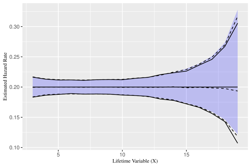
Figure 2: Theorem 3.1 left-truncation and right-censoring simulation study results: true quantities (solid line), empirical averages of 1,000 replicates of hazard rate estimates and corresponding empirical 95% log-scale confidence intervals (dashed lines), and the true 95% log-scale confidence interval using Theorem 3.1 (blue ribbon). All three closely agree.

We also verified Theorem 4.1 and Corollary 4.1.1 through a simulation study, but the results have been omitted in light of the proof in Appendix A.2. For interested readers, please contact the corresponding author for details.

6 Application

We now demonstrate the effectiveness of the cash flow modeling and pricing apparatus introduced in Section 4 in a realistic setting. Specifically, we will consider a large subset of lease data from the Mercedes-Benz Auto Lease Trust (MBALT) 2017-A consumer automobile lease asset-backed security (Mercedes-Benz, 2017). Because of the aforementioned SEC Regulation AB II enacted in November 2016 (Securities and Exchange Commission, 2014), investors may now obtain detailed loan-level borrower and monthly loan performance data through the Electronic Data Gather, Analysis, and Retrieval (EDGAR) system maintained by the SEC. For additional reference, Securities and Exchange Commission (2016) provides a detailed listing of available fields. MBALT 2017-A was placed in April of 2017 and closed in August of 2019. We thus have 28 months of loan performance and cash flow data. For convenience, we have made the downloaded and cleaned data file available in the online supplemental material.

The MBALT 2017-A transaction originally contained 56,402 lease contracts on Mercedes-Benz automobiles with original terms ranging from 24 to 60 months, the vast majority of which are 36 month leases (47,315). The credit profile of a substantial portion of underlying lessees is super-prime, which refers to a consumer credit score above 720 (Consumer Financial Protection Bureau, 2019). Nearly the entire pool of lessees would be classified as a prime credit, which refers to a consumer credit score above 660 (Consumer Financial Protection Bureau, 2019). Further, the majority of automobiles represent high-end or luxury vehicles. To see this, consider that the original vehicle value averages over just over $61,600. For a density plot of the lessee credit profile and vehicle values, see Figure 3. As another indicator of the low credit risk of this transaction, between 2012 and 2016, net losses as a percentage of average dollar amount of lease contracts outstanding for the Mercedes-Benz lease portfolio have ranged between 0.19% and 0.27% (Mercedes-Benz, 2017). We thus feel the MBALT 2017-A asset-backed security is a good candidate for the proposed model in Section 4, particularly in light of the discussion in Section 4.3.

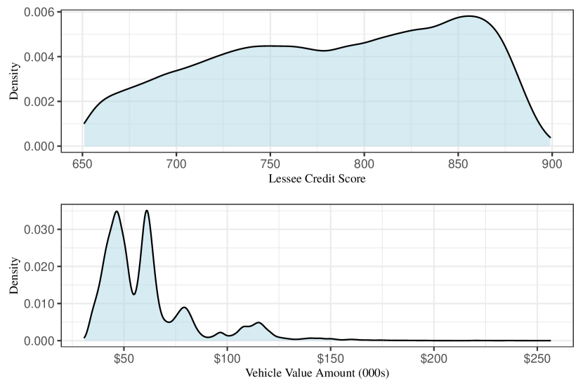
Figure 3: MBALT 2017-A credit and vehicle value distributions

6.1 Pricing results

For the remainder of the section, we will focus on a subset of the 47,315 36-month leases. Specifically, we removed 36-month lease contracts with data irregularities that could not be easily explained from a print out of cash flows or thorough review of data field descriptions. The first such irregularity was unclear or multiple residual payments. It is our opinion that some of the cash flows reported in the residual field (liquidationProceedsAmount) represent monthly payment cash flows, and they may be mislabeled as a form of bookkeeping convenience or error. To evaluate the potential of the cash flow model in Section 4 and avoid introducing potentially erroneous interpretations of the data, we have elected to remove such records. In total, this removed 16,741 contracts. In addition, there is a data field called terminationIndicator, and, in an additional 729 contracts, this field does not correspond to the month the final residual payment was received. These records were also removed. This leaves a total of 29,845 lease contracts. For an example of records removed in the form of Table 1, please see Appendix B. We recommend fitting a different set of hazard rate estimators (5) for each original lease termination length (i.e., 24-month leases should be fit separately from 36-month leases, and so on) because it is prudent to assume the prior information of the termination schedule will have a material impact on the underlying lifetime distribution. To price the complete trust, one may then add all different lease term groups together. For illustrative purposes, however, we will focus on the subset of 29,845 36-month lease contracts, which we will refer to as “the Trust” going forward.

The oldest lease in the Trust at initialization was 33 months old, and the youngest lease was 3 months old. Therefore, in the notation of Section 2, we have $\Delta=3$ and $m=30$. We will denote the lifetime random variable, $X$, as the time-until-contract-termination (i.e., the time the final residual payment is made to the Trust, see Table 1 as needed). We will first use the methods of Section 3 to estimate the distribution for $X$. To mimic the realities of pricing an active security, we will assume an observation window of 6, 12, 18, and 24 months. By an observation window, we mean that we will only use data from the first $\mathcal{O}$ months of securitization payments to estimate $X$, where $\mathcal{O}\in\{6,12,18,24\}$. If we make the connection to Figure 1, than an observation window of 6 months corresponds to $\varepsilon=39$. Estimates for the hazard rates of $X$ by observation window length may be found in Figure 4. We can see that the hazard rate accelerates close to month 36, which is expected for a lease contract with a scheduled termination of 36 months. It is also interesting to see the effect of left-truncation and right-censoring. For example, we cannot recover the distribution of $X$ before lease age 4 months. Given the pattern of the hazard rate in Figure 4, however, it is reasonable to assume the absence of months 1-3 will have a small impact on the overall results. In addition, we can see that as the observation window expands and less observations are right-censored, the right tail of $X$ gradually extends well beyond month 36. For the shortest observation window of 6 months, we observe terminations up to month 38, and, since $38\geq 36$, we assume $\xi=38$ in this case. Also of interest may be the resulting confidence intervals from Theorem 3.1, which are denoted by the blue ribbons in Figure 4. As we can see, the extended right tails have fewer observations and thus more estimator uncertainty than the early portions of the distribution of $X$.

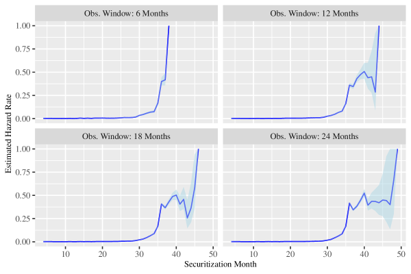
Figure 4: MBALT 2017-A hazard rate est. and 95% confidence intervals (36-Mo. leases).

To determine the pricing results, we calculate empirical estimates for $\mathbf{E}(Z\mid X=m)$ and $\displaystyle\Pr^{*}(D_{m}=k)$ for $k\in\{0,\ldots,\varphi\}$ and $m$ spanning the recoverable sample space of $X$, using only the observations available within the observation window. Note that to account for the small portion of defaults, we consider the difference between total residual realizations (liquidationProceedsAmount) and default losses or charge-offs (chargedOffAmount) when estimating the final residual payment made to the trust. Our objective is to use Corollary 4.1.1 for various values of $\kappa$ and compare the calculated price against the actual realized observations from the Trust. In addition, we will also compare the results of Corollary 4.1.1 against a variation of the modeling approach used in the MBALT 2017-A pricing prospectus (Mercedes-Benz, 2017, Appendix B); that is

Modeling Assumption: The cash flow schedules appearing in the immediately following tables were generated assuming that (i) the lessees make their remaining lease payments starting in March 2017 and every month thereafter until all scheduled lease payments are made and (ii) the residual value of the Leased Vehicles is due the month following the last related lease payment. (Mercedes-Benz, 2017, pg. B-1)

Specifically, we will compare the results of Corollary 4.1.1 against an approach that uses a non-random $X$ (i.e., all leases terminate at month 36 or immediately thereafter if older) but still uses the empirical estimates for $\mathbf{E}(Z\mid X=m)$. In other words, can our formulaic approach that accounts for left-truncation and right-censoring improve upon the non-random $X$ pricing assumptions of a newly issued auto-lease ABS? In Table 2, we refer to non-random $X$ as the Contract approach. To produce the comparisons, we utilized three interest-rate discount scenarios. The first is a simple zero-interest scenario, the second is a standard scenario, and the last is an inverted scenario. The exact spot rates used in each scenario may be found in Appendix B.

Based on the results in Table 2, we can see that Corollary 4.1.1 generally outperforms the contract approach and provides an accurate estimate of the value of future cash flows. More specifically, Corollary 4.1.1 is quite accurate over the short-term, even for an observation window of only 6 months. As the observation window increases, the results of Corollary 4.1.1 improve over a longer horizon as well, until they eventually are inside the Contract approach for all time horizons by an observation window of 12 months. As the observation window size increases, Corollary 4.1.1 begins to significantly outperform the Contract approach. The results hold generally across the three interest rate scenarios. Though not reported within this manuscript, we also note that the results are consistent with Table 2 for a subset of 24-month leases from the MBALT 2017-A transaction.

Because the results of Corollary 4.1.1 can be computed via a formula and do not require extensive simulation, we feel the ability to improve upon the non-random transaction prospectus approach (Mercedes-Benz, 2017, Appendix B) — especially as the observation window increases — at limited additional effort to be an advantage of our approach. Furthermore, the ability to estimate a fully specified asymptotic distribution of the hazard rate estimators using Theorem 3.1 — under the mutual independence assumption of $(X_{i},Y_{i})$ and $(X_{j},Y_{j})$ for $1\leq i\neq j\leq n$, which we feel is satisfied for the MBALT 2017-A pool of leases — allows for an assessment of the potential uncertainty of the pricing point estimates of Corollary 4.1.1. As such, we provide a demonstration in the following section.

		Zero Interest Rates					Standard Yield Curve					Inverted Yield Curve
Obs. Win.	$\kappa$	Con.	APV	Act.	Con.[%]	APV[%]	Con.	APV	Act.	Con.[%]	APV[%]	Con.	APV	Act.	Con.[%]	APV[%]
6 mo.	3	75	101	102	$-26.47$	$-$0.98	74	99	101	$-$26.73	$-$1.98	70	95	97	$-$27.84	$-$2.06
	6	169	210	205	$-$17.56	2.44	163	203	198	$-$17.68	2.53	153	190	186	$-$17.74	2.15
	9	258	317	310	$-$16.77	2.26	242	298	292	$-$17.12	2.05	225	277	271	$-$16.97	2.21
	12	359	436	420	$-$14.52	3.81	325	395	382	$-$14.92	3.40	302	367	355	$-$14.93	3.38
	15	466	567	553	$-$15.73	2.53	405	493	481	$-$15.80	2.49	378	461	450	$-$16.00	2.44
	18	629	716	671	$-$6.26	6.71	518	596	563	$-$7.99	5.86	489	562	530	$-$7.74	6.04
	21	770	860	792	$-$2.78	8.59	606	687	639	$-$5.16	7.51	581	656	609	$-$4.60	7.72
	22	804	911	837	$-$3.94	8.84	626	717	666	$-$6.01	7.66	602	688	638	$-$5.64	7.84
12 mo.	3	71	95	105	$-$32.38	$-$9.52	70	94	104	$-$32.69	$-$9.62	67	90	99	$-$32.32	$-$9.09
	6	159	204	215	$-$26.05	$-$5.12	154	197	208	$-$25.96	$-$5.29	144	185	195	$-$26.15	$-$5.13
	9	258	327	348	$-$25.86	$-$6.03	242	306	326	$-$25.77	$-$6.13	224	284	302	$-$25.83	$-$5.96
	12	408	463	466	$-$12.45	$-$0.64	364	417	423	$-$13.95	$-$1.42	338	387	392	$-$13.78	$-$1.28
	15	539	598	587	$-$8.18	1.87	462	519	513	$-$9.94	1.17	431	484	479	$-$10.02	1.04
	16	571	645	632	$-$9.65	2.06	485	552	545	$-$11.01	1.28	453	516	510	$-$11.18	1.18
18 mo.	3	66	108	133	$-$50.38	$-$18.80	65	106	131	$-$50.38	$-$19.08	62	102	125	$-$50.40	$-$18.40
	6	194	238	251	$-$22.71	$-$5.18	187	229	243	$-$23.05	$-$5.76	174	215	228	$-$23.68	$-$5.70
	9	317	370	371	$-$14.56	$-$0.27	296	347	351	$-$15.67	$-$1.14	273	322	326	$-$16.26	$-$1.23
	10	347	417	416	$-$16.59	0.24	322	386	389	$-$17.22	$-$0.77	297	358	361	$-$17.73	$-$0.83
24 mo.	3	84	118	120	$-$30.00	$-$1.67	83	116	119	$-$30.25	$-$2.52	79	111	114	$-$30.70	$-$2.63
	4	110	163	166	$-$33.73	$-$1.81	108	160	162	$-$33.33	$-$1.23	103	152	154	$-$33.12	$-$1.30

Table 2: MBALT 2017-A Corollary 4.1.1 pricing results (APV) comparison to prospectus approach (Mercedes-Benz, 2017) (Con.) and actual realized cash flows (Act.) including percentage differences for a pool of 29,845 36-month lease contracts. The results of Corollary 4.1.1 generally fall well within the prospectus approach, especially over short pricing horizons and as the observation window increases. The various discount interest rate curves may be found in Appendix B. All figures not in percentages are in millions.

6.2 Quantifying estimator uncertainty

In this section, we will illustrate how to use Theorem 3.1 to quantify the estimator uncertainty of price point estimates made with Corollary 4.1.1. Before proceeding, we first indicate that the mutual independence assumption of $(X_{i},Y_{i})$ and $(X_{j},Y_{j})$ for $1\leq i\neq j\leq n$ is likely satisfied for the MBALT 2017-A pool of leases (see Section 4.3 as needed). As a reminder, if an investor believed such an assumption was not satisfied, the results of this section may not be valid.

To obtain wider confidence intervals for illustrative purposes, we will consider 24-month lease contracts, which make up a smaller portion of MBALT 2017-A (866 leases out of a total of 50,402). The smaller sample is for illustrative purposes only; this analysis scales without issue. As in Section 6.1, we filtered the 866 24-lease contracts for data irregularities, which left 493 24-month lease contracts (see Appendix B as needed).

Figure 5 presents the resulting 95% confidence intervals for the hazard rate estimators using Theorem 3.1 for these 493 24-month lease contracts (compare with the 36-month contracts in Figure 4). The confidence intervals suggest that the hazard rate estimate random variables may reasonably fall within such intervals, which will naturally flow through the calculations in Corollary 4.1.1. From the work in Theorem 4.1, we can specify the exact distribution of the vector of hazard rate estimators, $\hat{\bm{\Lambda}}_{\tau,n}$, and use simulation to assess the potential variance of our APV estimates. That is, suppose we have a given observation window, say 6 months. Our procedure is as follows:

1. Determine $\hat{\bm{\Lambda}}_{\tau,n}$ using (5);

2. Estimate $\bm{\Sigma}$ from Theorem 3.1 using the estimators $\hat{f}_{*,\tau,n}$ and $\hat{U}_{\tau,n}$ defined in (5);

3. Use the delta-method (Mukhopadhyay, 2000, Theorem 5.3.5, pg. 261) to find the log-adjusted multivariate normal distribution (to ensure the confidence intervals for the hazard rates fall within 0 and 1);

4. For each of the desired number of replicates, simulate a realization of hazard rates from the multivariate normal distribution in [3] and then proceed to calculate $\text{APV}^{\kappa}_{\text{Trust}}$ from Corollary 4.1.1 with these simulated hazard rates;

5. Assess the potential estimation error though the distribution of stored results from [4].

We have done exactly this in Figure 5 for an observation window of 6 months, $\kappa=3$, 4,000 replicates, for the sample of 493 24-month leases from the MBALT 2017-A transaction described above. It is noteworthy the randomness of the hazard rate estimators can influence the pricing calculation of Corollary 4.1.1 by a range of over $1M, especially as the price was calculated to be approximately $5.4M. We also see the actual realization for these three months does fall within the range of simulated estimates. For this particular comparison, therefore, we would say that the estimation process of Section 3 in combination with the cash flow model of Section 4 was able to correctly predict the future cash flows.

We close this section with a remark on interpreting the results of Figure 5. As the sample size increases, we would expect the variability of the estimator to decrease by Theorem 3.1, which will lead to a more precise point estimate of the price using Corollary 4.1.1. This should not be conflated with less risk inherent in the future cash flows, however. The variability from the cash flows within (6) is due to the randomness of the lifetime random variable, $X$, and the delay and residual random variables, $D_{X}$ and $Z_{X}$, respectively. The volatility of these random variables will depend on the distributional estimates produced by the underlying data and not on the variability of the estimators themselves (though the latter may be of interest, too). Our process has produced an estimation and pricing process that we can expect to be asymptotically unbiased; it does not suggest that the cash flow risk will decline as $n$ grows.

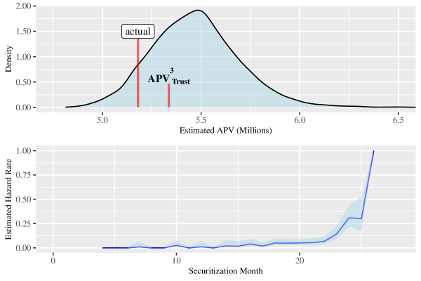
Figure 5: Illustrative example of Corollary 4.1.1 used to quantify estimator uncertainty. Data represents 493 24-month leases from MBALT 2017-A with an observation window of 6 months. The hazard rates and 95% confidence intervals fitted using Theorem 3.1 (see also Section 6.1). The distribution of price point estimates was created with 4,000 replications. The actual observed value and formulaic price $(\kappa=3)$ are denoted within the figure.

7 Conclusion

Despite life insurers significant holdings in securitized assets including ABS, it is difficult to find studies on this important fixed-income asset class within the actuarial literature. Further, current market pricing techniques for these assets either rely on a non-random time-to-event model or may not utilize the full asset-level disclosures of SEC Regulation AB II Securities and Exchange Commission (2014), which took effect in 2016. Our work fills this gap by establishing an effective pricing process that makes use of discrete-time survival analysis estimation techniques for incomplete data.

Broadly, there are two contributions of this article. The first contribution is the rigorous exposition of a framework capable of handling left-truncation and right-censoring in discrete-time in Section 2. This was necessary to derive the asymptotic properties of the hazard rate estimators assuming a discrete $X$, which we have done in Theorem 3.1 (statement in Section 3 and proof in Appendix A.1) for the first time in the case of left-truncation and right-censoring in the statistical literature. Note that this is a generalization of the results of Lautier et al. (2021), which was only valid for the case of left-truncation. The second contribution is the pricing formula of Theorem 4.1 (statement in Section 4 and proof in Appendix A.2), which is effectively an expected or actuarial present value that relies on the lifetime random variable distribution. The two contributions come together in that the distribution of the lifetime random variable may be estimated using the results of Section 3, and Theorem 3.1, under certain settings, may be used to assess the potential uncertainty of the pricing point estimator in Theorem 4.1. We also provide a discussion of when our model framework — in particular the key independence assumptions — is appropriate and inappropriate in Section 4.3. It is our opinion that the independence assumptions are reasonable in many realistic scenarios, but not all, such as with securitization pools of subprime credits.

The theoretical results of this paper are applied to a subset of 29,845 leases from the Mercedes-Benz 2017-A auto lease ABS bond in Section 6. Specifically in Section 6, we first provide discussion about why this particular bond meets both of the important independence assumptions of Section 4.3. Next, we found our formulaic pricing method, which accounts for the variability of the lease lifetime distribution, was capable of outperforming the standard modeling method within an auto lease ABS prospectus (Mercedes-Benz, 2017), which assumes a non-random lifetime distribution (Section 6.1, Table 2). Our illustrative application closed with a demonstration of how to use the asymptotic results of Theorem 3.1 to assess the price point estimator uncertainty of Theorem 4.1 (Section 6.2).

We recognize that other model formulations may attempt to connect economic variables to credit modeling at the loan level (Deng et al., 2000). These models typically find some association between consumer behavior and rational market behavior, such as the connection between prepayment behavior and the implicit “in-the-money” level a borrower finds himself with respect to his loan and home value. While some option-based models do have explanatory power, they are often not enough to fully explain the significant heterogeneity exhibited by borrowers (Deng et al., 2000). We have thus elected to use a data-based approach that models when lessees decide to terminate their leases rather than attempt to explain why lessees terminate their leases. The “when” is of paramount importance in a cash flow pricing exercise, and we find success with this approach in the realistic setting of Section 6. Fundamentally, therefore, our model produces a random timing and amount of cash flows at the individual lease contract level based on distributional estimations from historical performance. The most important of these distributions, the random time-until-contract-termination, may be estimated using the techniques of Section 3.

That said, we acknowledge that the “why” of consumer lessee behavior also has its merits, particularly in economically driven research. We postulate that a future version of the estimator (5) may be generalized to incorporate covariates, which could blend the “when” and “why” into a single model. Of particular interest may be the connection between current market interest rates and consumer behavior, especially for models of consumer loans or residential mortgages. At present, we leave this problem open to future research.

The results of this paper may be suitable for other forms of ABS besides auto lease bonds. One ideal generalization is agency MBS, which accounts for about $250 billion of life insurer assets (McMenamin et al., 2013). We recommend a generalization of the estimation framework of Sections 2 and 3 to the case of competing risks for securitized assets in which an investor would prefer to treat prepayment and default separately. Additional details may be found in Section 4.3. It is our opinion the combined estimation and pricing framework of this paper may be of use for insurance products, too, though we also leave this problem open for future research.

Appendix A Proofs

We first prove Theorem 3.1 and subsequently prove Theorem 4.1.

A.1 Proof of Theorem 3.1

We first define some helpful notation:

$$u_{\tau}(k,k^{\prime}) =\Pr(Y_{i}\leq k\leq\min(X_{i},C_{i}),Y_{i}\leq k^{\prime}\leq\min(X_{i},C_{i}))$$

$$=\Pr(Y_{i}\leq\min(k,k^{\prime}),\max(k,k^{\prime})\leq X_{i},\max(k,k^{\prime})\leq C_{i})$$

$$=\Pr(Y\leq\min(k,k^{\prime}),X\geq\max(k,k^{\prime}),C\geq\max(k,k^{\prime})\mid X\geq Y)$$

$$=\Pr(Y\leq\min(k,k^{\prime}),X\geq\max(k,k^{\prime}),C\geq\max(k,k^{\prime}),X\geq Y)/\Pr(X\geq Y)$$

$$=\Pr(Y\leq\min(k,k^{\prime}),X\geq\max(k,k^{\prime}),C\geq\max(k,k^{\prime}))/\alpha$$

$$=\frac{1}{\alpha}\Pr(X\geq\max(k,k^{\prime}))\Pr(Y\leq\min(k,k^{\prime}),\max(k,k^{\prime})\leq C).$$ (11)

Notice $u_{\tau}(k,k^{\prime})=u_{\tau}(k^{\prime},k)$ and $u_{\tau}(k,k)=U_{\tau}(k)$. Further,

$$r_{\tau}(k,k^{\prime}) =\Pr(X_{i}=\max(k,k^{\prime}),Y_{i}\leq\min(k,k^{\prime}),X_{i}\leq C_{i})$$

$$=\Pr(X=\max(k,k^{\prime}),Y\leq\min(k,k^{\prime}),X\leq C\mid X\geq Y)$$

$$=\Pr(X=\max(k,k^{\prime}),Y\leq\min(k,k^{\prime}),X\leq C,X\geq Y)/\Pr(X\geq Y)$$

$$=\Pr(X=\max(k,k^{\prime}),Y\leq\min(k,k^{\prime}),C\geq\max(k,k^{\prime}))/\alpha$$

$$=\frac{1}{\alpha}\Pr(X=\max(k,k^{\prime}))\Pr(Y\leq\min(k,k^{\prime}),\max(k,k^{\prime})\leq C).$$ (12)

Notice $r_{\tau}(k,k^{\prime})=r_{\tau}(k^{\prime},k)$ and $r_{\tau}(k,k)=f_{*,\tau}(k)$. We first state a lemma, and the proof of Theorem 3.1 follows.

Lemma 1 ($\hat{\mathbf{U}}_{\tau,n}$ Asymptotic Properties).

Define $\hat{\mathbf{U}}_{\tau,n}=\big{(}\hat{U}_{\tau,n}(\Delta+1),\ldots,\hat{U}_{\tau,n}(\xi)\big{)}^{\top}$, where $\hat{U}_{\tau,n}$ follows from (5). Then,

1. $$\hat{\mathbf{U}}_{\tau,n}\overset{\mathcal{P}}{\longrightarrow}\mathbf{U}_{\tau},\text{ as }n\rightarrow\infty;$$

2. $$\sqrt{n}(\hat{\mathbf{U}}_{\tau,n}-\mathbf{U}_{\tau})\overset{\mathcal{L}}{\longrightarrow}N(\mathbf{0},\mathbf{\Sigma}_{u}),\text{ as }n\rightarrow\infty,$$

where $\mathbf{U}_{\tau}=(U_{\tau}(\Delta+1),\ldots,U_{\tau}(\xi))^{\top}$ with $U_{\tau}$ as defined in (4) and $\bm{\Sigma}_{u}$ is a covariance matrix $\lVert\sigma_{k^{\prime},k}\rVert$ such that

$$\sigma_{k^{\prime},k}=\begin{cases}U_{\tau}(k)[1-U_{\tau}(k)],&k^{\prime}=k\\ u_{\tau}(k^{\prime},k)-U_{\tau}(k^{\prime})U_{\tau}(k),&k^{\prime}\neq k\end{cases},$$

for $k^{\prime},k=\Delta+1,\ldots,\xi$.

Proof.

Statement (i) follows from (ii), so it is left to show (ii). Observe

$$\hat{\mathbf{U}}_{\tau,n}=\begin{bmatrix}\hat{U}_{\tau,n}(\Delta+1)\\ \vdots\\ \hat{U}_{\tau,n}(\xi)\end{bmatrix}=\begin{bmatrix}\displaystyle\frac{1}{n}\sum_{i=1}^{n}\mathbf{1}_{Y_{i}\leq\Delta+1\leq\min(X_{i},C_{i})}\\ \vdots\\ \displaystyle\frac{1}{n}\sum_{i=1}^{n}\mathbf{1}_{Y_{i}\leq\xi\leq\min(X_{i},C_{i})}\end{bmatrix}=\frac{1}{n}\sum_{i=1}^{n}\begin{bmatrix}Y_{\tau,\Delta+1(i)}\\ \vdots\\ Y_{\tau,\xi(i)}\end{bmatrix},$$

where $Y_{\tau,k(i)}$, $\Delta+1\leq k\leq\xi$ are independent and identically distributed Bernoulli random variables with probability of success given by

$$\Pr(Y_{i}\leq k\leq\min(X_{i},C_{i}))=\Pr(Y\leq k\leq\min(X,C)\mid X\geq Y)=U_{\tau}(k),$$

for $k=\Delta+1,\ldots,\xi$. Thus, $E[Y_{\tau,k(i)}]=U_{\tau}(k)$ and $\text{Var}[Y_{\tau,k(i)}]=U_{\tau}(k)(1-U_{\tau}(k))$. Now, since

$$\mathbf{1}_{Y_{i}\leq k^{\prime}\leq\min(X_{i},C_{i})}\mathbf{1}_{Y_{i}\leq k\leq\min(X_{i},C_{i})}=\mathbf{1}_{Y_{i}\leq\min(k^{\prime},k),X_{i}\geq\max(k^{\prime},k),C_{i}\geq\max(k^{\prime},k)},$$

we have

$$E[Y_{\tau,k^{\prime}(i)}Y_{\tau,k(i)}]=E[\mathbf{1}_{Y_{i}\leq\min(k^{\prime},k),X_{i}\geq\max(k^{\prime},k),C_{i}\geq\max(k^{\prime},k)}]=u_{\tau}(k^{\prime},k),$$ (13)

for $k^{\prime},k=\Delta+1,\ldots,\xi$. Thus,

$$\text{Cov}[Y_{\tau,k^{\prime}(i)}Y_{\tau,k(i)}] =E[Y_{\tau,k^{\prime}(i)}Y_{\tau,k(i)}]-E[Y_{\tau,k^{\prime}(i)}]E[Y_{\tau,k(i)}]$$

$$=u_{\tau}(k^{\prime},k)-U_{\tau}(k^{\prime})U_{\tau}(k).$$

Recall that (13) reduces to $U_{\tau}(k)$ when $k^{\prime}=k$. Use the multivariate Central Limit Theorem (Lehmann and Casella, 1998, Theorem 8.21, pg. 61) to complete the proof. ∎

We now prove Theorem 3.1.

Proof.

Statement (i) follows from (ii), so it is left to show (ii). Let $\Delta+1\leq k\leq\xi$ and observe $\mathbf{1}_{X_{i}\leq C_{i}}\mathbf{1}_{\min(X_{i},C_{i})=k}=\mathbf{1}_{X_{i}=k,X_{i}\leq C_{i}}$ and so

$$\hat{\lambda}_{\tau,n}(k)-\lambda_{\tau}(k) =\frac{\frac{1}{n}\sum_{i=1}^{n}\mathbf{1}_{X_{i}=k,X_{i}\leq C_{i}}}{\hat{U}_{\tau,n}(k)}-\frac{f_{*,\tau}(k)}{U_{\tau}(k)}$$

$$=\frac{\frac{1}{n}\sum_{i=1}^{n}\mathbf{1}_{X_{i}=k,X_{i}\leq C_{i}}U_{\tau}(k)-f_{*,\tau}(k)\hat{U}_{\tau,n}(k)}{\hat{U}_{\tau,n}(k)U_{\tau}(k)}$$

$$=\bigg{[}\frac{1}{\hat{U}_{\tau,n}(k)U_{\tau}(k)}\bigg{]}\frac{1}{n}\sum_{i=1}^{n}\{\mathbf{1}_{X_{i}=k,X_{i}\leq C_{i}}U_{\tau}(k)-f_{*,\tau}(k)\mathbf{1}_{Y_{i}\leq k\leq\min(X_{i},C_{i})}\}.$$

Further define

$$Z_{\tau,k(i)}=\mathbf{1}_{X_{i}=k,X_{i}\leq C_{i}}U_{\tau}(k)-f_{*,\tau}(k)\mathbf{1}_{Y_{i}\leq k\leq\min(X_{i},C_{i})}.$$

Hence,

$$\hat{\bm{\Lambda}}_{\tau,n}-\bm{\Lambda}_{\tau}=\mathbf{A}_{\tau,n}\frac{1}{n}\sum_{i=1}^{n}\begin{bmatrix}Z_{\tau,\Delta+1(i)}\\ \vdots\\ Z_{\tau,\xi(i)}\end{bmatrix},$$

where $\mathbf{A}_{\tau,n}=\text{diag}([\hat{U}_{\tau,n}(\Delta+1)U_{\tau}(\Delta+1)]^{-1},\ldots,[\hat{U}_{\tau,n}(\xi)U_{\tau}(\xi)]^{-1})$. That is,

$$\hat{\bm{\Lambda}}_{n}-\bm{\Lambda}=\mathbf{A}_{\tau,n}\frac{1}{n}\sum_{i=1}^{n}\mathbf{Z}_{\tau,(i)},$$

where $\mathbf{Z}_{\tau,(i)}=(Z_{\tau,\Delta+1(i)},\ldots,Z_{\tau,\xi(i)})^{\top}$, $1\leq i\leq n$ are independent and identically distributed random vectors. We will also subsequently show that the components of random vector $\mathbf{Z}_{\tau,(i)}$ are uncorrelated.

First notice $\mathbf{1}_{X_{i}=k,X_{i}\leq C_{i}}$ is a Bernoulli random variable with probability parameter $f_{*,\tau}(k)$. Similarly, $\mathbf{1}_{Y_{i}\leq k\leq\min(X_{i},C_{i})}$ is a Bernoulli random variable with probability parameter $U_{\tau}(x)$. Thus,

$$E[Z_{\tau,k(i)}] =E[\mathbf{1}_{X_{i}=k,X_{i}\leq C_{i}}]U_{\tau}(k)-f_{*,\tau}(k)E[\mathbf{1}_{Y_{i}\leq k\leq\min(X_{i},C_{i})}]$$

$$=f_{*,\tau}(k)U_{\tau}(k)-f_{*,\tau}(k)U_{\tau}(k)$$

$$=0.$$

We now show

$$\text{Cov}[Z_{k(i)},Z_{k^{\prime}(i)}]=\begin{cases}U_{\tau}(k)f_{*,\tau}(k)[U_{\tau}(k)-f_{*,\tau}(k)],&k=k^{\prime}\\ 0,&k\neq k^{\prime}.\end{cases}$$ (14)

Since $E[Z_{\tau,k(i)}]=0$, we have

$$\text{Cov}[Z_{\tau,k(i)},Z_{\tau,k^{\prime}(i)}]={} E[Z_{\tau,k(i)}Z_{\tau,k^{\prime}(i)}]$$

$$={} E\bigg{[}\bigg{(}\mathbf{1}_{X_{i}=k,X_{i}\leq C_{i}}U_{\tau}(k)-f_{*,\tau}(k)\mathbf{1}_{Y_{i}\leq k\leq\min(X_{i},C_{i})}\bigg{)}$$

$$\bigg{(}\mathbf{1}_{X_{i}=k^{\prime},X_{i}\leq C_{i}}U_{\tau}(k^{\prime})-f_{*,\tau}(k^{\prime})\mathbf{1}_{Y_{i}\leq k^{\prime}\leq\min(X_{i},C_{i})}\bigg{)}\bigg{]}$$

$$={} U_{\tau}(k)U_{\tau}(k^{\prime})E[\mathbf{1}_{X_{i}=k,X_{i}\leq C_{i}}\mathbf{1}_{X_{i}=k^{\prime},X_{i}\leq C_{i}}]$$

$$-f_{*,\tau}(k)U_{\tau}(k^{\prime})E[\mathbf{1}_{Y_{i}\leq k\leq\min(X_{i},C_{i})}\mathbf{1}_{X_{i}=k^{\prime},X_{i}\leq C_{i}}]$$

$$-f_{*,\tau}(k^{\prime})U_{\tau}(k)E[\mathbf{1}_{Y_{i}\leq k^{\prime}\leq\min(X_{i},C_{i})}\mathbf{1}_{X_{i}=k,X_{i}\leq C_{i}}]$$

$$+f_{*,\tau}(k)f_{*,\tau}(k^{\prime})E[\mathbf{1}_{Y_{i}\leq k\leq\min(X_{i},C_{i})}\mathbf{1}_{Y_{i}\leq k^{\prime}\leq\min(X_{i},C_{i})}]$$

We proceed by cases.

Case 1: $k=k^{\prime}$.

Since $\mathbf{1}_{X_{i}=k,X_{i}\leq C_{i}}\mathbf{1}_{X_{i}=k^{\prime},X_{i}\leq C_{i}}=\mathbf{1}_{X_{i}=k,X_{i}\leq C_{i}}$, $E[\mathbf{1}_{X_{i}=k,X_{i}\leq C_{i}}\mathbf{1}_{X_{i}=k^{\prime},X_{i}\leq C_{i}}]=f_{*,\tau}(k)$. Additionally,

$$\mathbf{1}_{Y_{i}\leq k\leq\min(X_{i},C_{i})}\mathbf{1}_{X_{i}=k^{\prime},X_{i}\leq C_{i}} =\mathbf{1}_{Y_{i}\leq k^{\prime}\leq\min(X_{i},C_{i})}\mathbf{1}_{X_{i}=k,X_{i}\leq C_{i}}$$

$$=\mathbf{1}_{Y_{i}\leq k\leq\min(X_{i},C_{i}),X_{i}=k,X_{i}\leq C_{i}}$$

$$=\mathbf{1}_{Y_{i}\leq X_{i}\leq X_{i},X_{i}=k,X_{i}\leq C_{i}}$$

$$=\mathbf{1}_{X_{i}=k,X_{i}\leq C_{i}}.$$

Therefore,

$$E[\mathbf{1}_{Y_{i}\leq k\leq\min(X_{i},C_{i})}\mathbf{1}_{X_{i}=k^{\prime},X_{i}\leq C_{i}}]=E[\mathbf{1}_{Y_{i}\leq k^{\prime}\leq\min(X_{i},C_{i})}\mathbf{1}_{X_{i}=k,X_{i}\leq C_{i}}]=f_{*,\tau}(k).$$

Finally,

$$\mathbf{1}_{Y_{i}\leq k\leq\min(X_{i},C_{i})}\mathbf{1}_{Y_{i}\leq k^{\prime}\leq\min(X_{i},C_{i})}=\mathbf{1}_{Y_{i}\leq k\leq\min(X_{i},C_{i})}.$$

Thus, $E[\mathbf{1}_{Y_{i}\leq k\leq\min(X_{i},C_{i})}\mathbf{1}_{Y_{i}\leq k^{\prime}\leq\min(X_{i},C_{i})}]=U_{\tau}(k)$. Replace these expectations in $E[Z_{k(i)}Z_{k^{\prime}(i)}]$ to write

$$\text{Cov}[Z_{k(i)},Z_{k^{\prime}(i)}]=U_{\tau}(k)f_{*,\tau}(k)[U_{\tau}(k)-f_{*,\tau}(k)].$$

Case 2: $k\neq k^{\prime}$.

Since $\mathbf{1}_{X_{i}=k,X_{i}\leq C_{i}}\mathbf{1}_{X_{i}=k^{\prime},X_{i}\leq C_{i}}=0$, $E[\mathbf{1}_{X_{i}=k,X_{i}\leq C_{i}}\mathbf{1}_{X_{i}=k^{\prime},X_{i}\leq C_{i}}]=0$. Assume $k<k^{\prime}$. Then

$$\mathbf{1}_{Y_{i}\leq k\leq\min(X_{i},C_{i})}\mathbf{1}_{X_{i}=k^{\prime},X_{i}\leq C_{i}} =\mathbf{1}_{Y_{i}\leq k\leq\min(X_{i},C_{i}),X_{i}=k^{\prime},X_{i}\leq C_{i}}$$

$$=\mathbf{1}_{Y_{i}\leq k,X_{i}=k^{\prime},X_{i}\leq C_{i}}.$$

Therefore, $E[\mathbf{1}_{Y_{i}\leq k\leq\min(X_{i},C_{i})}\mathbf{1}_{X_{i}=k^{\prime},X_{i}\leq C_{i}}]=\Pr(X_{i}=k^{\prime},Y_{i}\leq k,X_{i}\leq C_{i})$. Further, when $k<k^{\prime}$

$$\mathbf{1}_{Y_{i}\leq k^{\prime}\leq\min(X_{i},C_{i})}\mathbf{1}_{X_{i}=k,X_{i}\leq C_{i}}=\mathbf{1}_{Y_{i}\leq k^{\prime}\leq\min(X_{i},C_{i}),X_{i}=k,X_{i}\leq C_{i}}=0.$$

Thus, $E[\mathbf{1}_{Y_{i}\leq k^{\prime}\leq\min(X_{i},C_{i})}\mathbf{1}_{X_{i}=k,X_{i}\leq C_{i}}]=0$. Now, if instead $k>k^{\prime}$, then by symmetry,

$$E[\mathbf{1}_{Y_{i}\leq k^{\prime}\leq\min(X_{i},C_{i})}\mathbf{1}_{X_{i}=k,X_{i}\leq C_{i}}]=\Pr(X_{i}=k,Y_{i}\leq k^{\prime},X_{i}\leq C_{i}),$$

and $E[\mathbf{1}_{Y_{i}\leq k\leq\min(X_{i},C_{i})}\mathbf{1}_{X_{i}=k^{\prime},X_{i}\leq C_{i}}]=0$. Thus, we can generalize and claim

$$f_{*,\tau}(k)U_{\tau}(k^{\prime})E[\mathbf{1}_{Y_{i}\leq k\leq\min(X_{i},C_{i})}\mathbf{1}_{X_{i}=k^{\prime},X_{i}\leq C_{i}}]+f_{*,\tau}(k^{\prime})U_{\tau}(k)E[\mathbf{1}_{Y_{i}\leq k\leq\min(X_{i},C_{i})}\mathbf{1}_{X_{i}=k^{\prime},X_{i}\leq C_{i}}]$$

$$= f_{*,\tau}(\min(k,k^{\prime}))U_{\tau}(\max(k,k^{\prime}))r_{\tau}(k,k^{\prime}).$$

Lastly, notice $E[\mathbf{1}_{Y_{i}\leq k\leq\min(X_{i},C_{i})}\mathbf{1}_{Y_{i}\leq k^{\prime}\leq\min(X_{i},C_{i})}]=u_{\tau}(k,k^{\prime})$. Replace these expectations in $E[Z_{k(i)}Z_{k^{\prime}(i)}]$ to write

$$\text{Cov}(Z_{k(i)},Z_{k^{\prime}(i)})={} -f_{*,\tau}(\min(k,k^{\prime}))U_{\tau}(\max(k,k^{\prime}))r_{\tau}(k,k^{\prime})$$

$$+f_{*,\tau}(\min(k,k^{\prime}))f_{*,\tau}(\max(k,k^{\prime}))u_{\tau}(k,k^{\prime})$$

$$={} f_{*,\tau}(\min(k,k^{\prime}))\{f_{*,\tau}(\max(k,k^{\prime}))u_{\tau}(k,k^{\prime})-r_{\tau}(k,k^{\prime})U_{\tau}(\max(k,k^{\prime}))\}.$$

However, using (11) and (12),

$$f_{*,\tau}(\max(k,k^{\prime}))u_{\tau}(k,k^{\prime}) =\bigg{[}\frac{\Pr(X=\max(k,k^{\prime}))\Pr(Y\leq\max(k,k^{\prime})\leq C)}{\alpha}\bigg{]}$$

$$\times\Bigg{[}\frac{\Pr(X\geq\max(k,k^{\prime}))\Pr(Y\leq\max(k,k^{\prime}),\max(k,k^{\prime})\leq C)}{\alpha}\bigg{]}$$

$$=\bigg{[}\frac{\Pr(X=\max(k,k^{\prime}))\Pr(Y\leq\min(k,k^{\prime}),\max(k,k^{\prime})\leq C)}{\alpha}\bigg{]}$$

$$\times\bigg{[}\frac{\Pr(X\geq\max(k,k^{\prime}))\Pr(Y\leq\max(k,k^{\prime})\leq C)}{\alpha}\bigg{]}$$

$$=r_{\tau}(k,k^{\prime})U_{\tau}(\max(k,k^{\prime})).$$

Thus, $\text{Cov}[Z_{k(i)},Z_{k^{\prime}(i)}]=0$ when $k\neq k^{\prime}$. This confirms (14). Now define

$$\mathbf{D}_{\tau}=\text{diag}\big{(}U_{\tau}(\Delta+1)f_{*,\tau}(\Delta+1)[U_{\tau}(\Delta+1)-f_{*,\tau}(\Delta+1)],\ldots,U_{\tau}(\xi)f_{*,\tau}(\xi)[U_{\tau}(\xi)-f_{*,\tau}(\xi)]\big{)},$$

and

$$\bar{\mathbf{Z}}_{\tau,n}=\frac{1}{n}\sum_{i=1}^{n}\mathbf{Z}_{\tau,(i)}.$$

Thus, by the multivariate Central Limit Theorem (Lehmann and Casella, 1998, Theorem 8.21, pg. 61) we may claim

$$\sqrt{n}(\bar{\mathbf{Z}}_{\tau,n}-\bm{0})\overset{\mathcal{L}}{\longrightarrow}N(\bm{0},\mathbf{D}_{\tau}),\text{ as }n\rightarrow\infty.$$

Next define

$$\mathbf{V}_{\tau}=\text{diag}\big{(}U_{\tau}(\Delta+1)^{-2},\ldots,U_{\tau}(\xi)^{-2}),$$

and use Lemma 1 to claim $\mathbf{A}_{\tau,n}\overset{\mathcal{P}}{\longrightarrow}\mathbf{V}_{\tau}$, as $n\rightarrow\infty$. Therefore, by multivariate Slutsky’s Theorem (Lehmann and Casella, 1998, Theorem 5.1.6, pg. 283),

$$\sqrt{n}\big{(}\mathbf{A}_{\tau,n}\bar{\mathbf{Z}}_{\tau,n}\big{)}\overset{\mathcal{L}}{\longrightarrow}N(\bm{0},\mathbf{V}_{\tau}\mathbf{D}_{\tau}\mathbf{V}_{\tau}^{\top})\text{ as }n\rightarrow\infty.$$

Finally, observe $\mathbf{V}_{\tau}\mathbf{D}_{\tau}\mathbf{V}_{\tau}^{\top}=\bm{\Sigma}$ and $\mathbf{A}_{\tau,n}\bar{\mathbf{Z}}_{\tau,n}=\hat{\bm{\Lambda}}_{\tau,n}-\bm{\Lambda}_{\tau}$ to complete the proof. ∎

A.2 Proof of Theorem 4.1

Proof.

By repeated use of law of total expectation (Mukhopadhyay, 2000, Theorem 3.3.1, pg. 112) and (6),

$$\text{APV}_{i}=\mathbf{E}[\text{PV}_{i}]=\mathbf{E}_{X}\{\mathbf{E}_{D}[\mathbf{E}_{Z}(\text{PV}_{i}\mid X_{i},D_{X_{i}})\mid X_{i}]\}.$$ (15)

Now,

$$\mathbf{E}_{Z}(\text{PV}_{i}\mid X_{i},D_{X_{i}})=W_{i}(X_{i},D_{X_{i}})+R_{i}(X_{i})\mathbf{E}(Z\mid X=X_{i}).$$

Thus,

$$\mathbf{E}_{D}[\mathbf{E}_{Z}(\text{PV}_{i}\mid X_{i},D_{X_{i}})\mid X_{i}] =\mathbf{E}_{D}\bigg{[}W_{i}(X_{i},D_{X_{i}})+R_{i}(X_{i})\mathbf{E}(Z\mid X=X_{i})\bigg{|}X_{i}\bigg{]}$$

$$=\mathbf{E}_{D}[W_{i}(X_{i},D_{X_{i}})\mid X_{i}]+R_{i}(X_{i})\mathbf{E}(Z\mid X=X_{i})$$

$$=\bigg{\{}\sum_{k=0}^{\varphi}W_{i}(X_{i},k)\Pr^{*}(D_{m}=k)\bigg{\}}+R_{i}(X_{i})\mathbf{E}(Z\mid X=X_{i}).$$

Hence, returning to (15)

$$\text{APV}_{i} =\mathbf{E}_{X}\{\mathbf{E}_{D}[\mathbf{E}_{Z}(\text{PV}_{i}\mid X_{i},D_{X_{i}})\mid X_{i}]\}$$

$$=\mathbf{E}_{X}\bigg{[}\bigg{\{}\sum_{k=0}^{\varphi}W_{i}(X_{i},k)\Pr^{*}(D_{m}=k)\bigg{\}}+R_{i}(X_{i})\mathbf{E}(Z\mid X=X_{i})\bigg{]}$$

$$=\sum_{m=x_{\varepsilon(i)}}^{\xi}\bigg{(}\bigg{\{}\sum_{k=0}^{\varphi}W_{i}(m,k)\Pr^{*}(D_{m}=k)\bigg{\}}+R_{i}(m)\mathbf{E}(Z\mid X=m)\bigg{)}p_{x_{\varepsilon(i)}}^{m}.$$

The proof is complete by the linear property of expectations (Mukhopadhyay, 2000, Theorem 3.3.2, pg. 116). ∎

Appendix B Extended application details

The following information pertains to Section 6.

Observed data irregularities

Per the opening discussion of Section 6.1, some records were removed due to difficulties interpreting the reported cash flows. In this section, we present examples of two such records in Table 3.

For example asset number 3, we can see that there are two positive payments in the residual column (liquidationProceedsAmount). While it appears the smaller payment of 3,728 at age 37 represents approximately nine monthly payments of 417, it is not clearly indicated in the data. Modeling such a lease contract will require making assumptions about the payment of 3,728 that we cannot verify. Instead, as the model of Section 4 is a new proposal, we have attempted to remove the potential confounding effects of data irregularities and focused on demonstrating the model is capable of pricing cash flows that follow a clear pattern, such as those in Table 1.

For example asset number 4, we see two large residual payments at ages 32 and 40. Further, we see that the termination indicator (terminationIndicator) occurs at age 35, despite the large residual payment occurring later, at age 40. This cash flow pattern is very difficult to translate accurately from the reported data into a lease contract outcome without more information.

	Ex. Asset Num: 3				Ex. Asset Num: 4
Obs. Month	Age	Pmt	Resid.	Term. Ind.	Age	Pmt	Resid.	Term. Ind.
1	30	834	0	–	30	4,315	0	–
2	31	417	0	–	31	0	0	–
3	32	417	0	–	32	2,157	20,194	–
4	33	417	0	–	33	0	0	–
5	34	417	0	–	34	0	0	–
6	35	0	0	–	35	0	0	1
7	36	807	0	–	36	0	0	–
8	37	416	3,728	–	37	0	0	–
9	38	0	0	–	38	0	0	–
10	39	0	14,974	1	39	0	0	–
11	–	–	–	–	40	0	36,934	–

Table 3: MBALT 2017-A sample lives of cash flow data irregularities

Interest rate scenarios

Figure 6 presents the two non-zero interest rate scenarios for the results of Section 6.

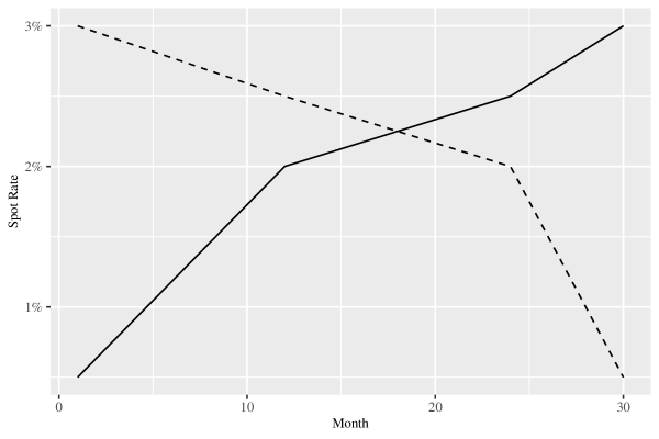
Figure 6: Spot rates for Section 6; standard (solid), inverted (dashed)

References

- Bluhm et al. (2010) C. Bluhm, L. Overbeck and C. Wagner (2010). Introduction to Credit Risk Modeling, Second Edition. Boca Raton, Florida: Chapman & Hall/CRC.
- Chiu and Wong (2014) M. C. Chiu and H. Y. Wong (2014). “Mean–variance asset–liability management with asset correlation risk and insurance liabilities.” Insurance: Mathematics and Economics 59, 300–310.
- Consumer Financial Protection Bureau (2019) Consumer Financial Protection Bureau (2019). “Borrower risk profiles.” https://www.consumerfinance.gov/data-research/consumer-credit-trends/auto-loans/borrower-risk-profiles/ (Accessed: 2022-06-15).
- Davidson and Levin (2014) A. Davidson and A. Levin (2014). Mortgage Valuation Models: Embedded Options, Risk, and Uncertainty. New York, New York: Oxford University Press.
- Demyanyk and Van Hemert (2009) Y. Demyanyk and O. Van Hemert (2009). “Understanding the subprime mortgage crisis.” The Review of Financial Studies 24, 1848–1880.
- Deng et al. (2000) Y. Deng, J. M. Quigley and R. Van Order (2000). “Mortgage terminations, heterogeneity and the exercise of mortgage options.” Econometrica 68, 275–307.
- Denuit et al. (2015) M. Denuit, A. Kiriliouk and J. Segers (2015). “Max-factor individual risk models with application to credit portfolios.” Insurance: Mathematics and Economics 62, 162–172.
- Dickson et al. (2020) D. C. Dickson, M. R. Hardy and H. R. Waters (2020). Actuarial Mathematics for Life Contingent Risks. Cambridge, United Kingdom: Cambridge University Press, 3 edition.
- Fermanian (2013) J.-D. Fermanian (2013). “A top-down approach for asset-backed securities: A consistent way of managing prepayment, default and interest rate risks.” The Journal of Real Estate Finance and Economics 46, 480–515.
- Gatzert and Martin (2012) N. Gatzert and M. Martin (2012). “Quantifying credit and market risk under Solvency II: Standard approach versus internal model.” Insurance: Mathematics and Economics 51, 649–666.
- Guo et al. (2017) N. Guo, F. Wang and J. Yang (2017). “Remarks on composite Bernstein copula and its application to credit risk analysis.” Insurance: Mathematics and Economics 77, 38–48.
- Jang et al. (2018) J. Jang, A. Dassios and H. Zhao (2018). “Moments of renewal shot-noise processes and their applications.” Scandinavian Actuarial Journal 2018, 727–752.
- Kiatsupaibul et al. (2017) S. Kiatsupaibul, A. J. Hayter and S. Somsong (2017). “Confidence sets and confidence bands for a beta distribution with applications to credit risk management.” Insurance: Mathematics and Economics 75, 98–104.
- Klein and Moeschberger (2003) J. P. Klein and M. L. Moeschberger (2003). Survival Analysis: Techniques for Censored and Truncated Data. Springer.
- Klugman et al. (2012) S. A. Klugman, H. H. Panjer and G. E. Willmot (2012). Loss Models: From Data to Decisions, Fourth Edition. Hoboken, New Jersey: John Wiley & Sons, Inc.
- Lautier et al. (2021) J. P. Lautier, V. Pozdnyakov and J. Yan (2021). “Estimating a distribution function for discrete data subject to random truncation with an application to structured finance.” https://doi.org/10.48550/arXiv.2108.04854.
- Lehmann and Casella (1998) E. Lehmann and G. Casella (1998). Theory of Point Estimation, 2nd Edition. Springer.
- Li et al. (2018) D. Li, Y. Shen and Y. Zeng (2018). “Dynamic derivative-based investment strategy for mean–variance asset–liability management with stochastic volatility.” Insurance: Mathematics and Economics 78, 72–86. Longevity risk and capital markets: The 2015–16 update.
- Liang and Wang (2012) X. Liang and G. Wang (2012). “On a reduced form credit risk model with common shock and regime switching.” Insurance: Mathematics and Economics 51, 567–575.
- McMenamin et al. (2013) R. McMenamin, A. L. Paulson, T. Plestis and R. J. Rosen (2013). “Chicago Fed Letter: What do U.S. life insurers invest in?” Essays on Issues, The Federal Reserve Bank of Chicago 309, 1–4.
- Mercedes-Benz (2017) Mercedes-Benz (2017). “Prospectus.” https://www.sec.gov/Archives/edgar/data/1537805/000114036117016403/form424b2.htm (Accessed: 2022-08-18).
- Mercedes-Benz (2021) Mercedes-Benz (2021). “Prospectus.” https://www.sec.gov/Archives/edgar/data/1537805/000114036121022216/brhc10026152_424b2.htm (Accessed: 2022-08-18).
- Mukhopadhyay (2000) N. Mukhopadhyay (2000). Probability and Statistical Inference. New York, NY: Marcel Dekker.
- National Association of Insurance Commissioners (2020) National Association of Insurance Commissioners (2020). “Statistical compilation of annual statement information for life/fraternal insurance companies in 2019.” https://content.naic.org/sites/default/files/publication-sta-ls-life.pdf (Accessed: 2022-09-15).
- Neilson et al. (2022) J. J. Neilson, S. G. Ryan, K. P. Wang and B. Xie (2022). “Asset-level transparency and the (e)valuation of asset-backed securities.” Journal of Accounting Research 60, 1131–1183.
- Nolsøe et al. (2020) K. A. Nolsøe, D. Degrijse, S. Ahm, K. Brix, M. Storgaard and J. Strodl (2020). “Cash flow techniques for asset liability management.” Scandinavian Actuarial Journal 2020, 196–217.
- Securities and Exchange Commission (2014) Securities and Exchange Commission (2014). “17 CFR Parts 229, 230, 232, 239, 240, 243, and 249 Asset-Backed Securities Disclosure and Registration.”
- Securities and Exchange Commission (2016) Securities and Exchange Commission (2016). “17 CFR §229.1125 (Item 1125) Schedule AL - Asset-level information.”
- Tsai et al. (1987) W.-Y. Tsai, N. P. Jewell and M.-C. Wang (1987). “A note on the product-limit estimator under right censoring and left truncation.” Biometrika 74, 883–886.
- Tuckman and Serrat (2012) B. Tuckman and A. Serrat (2012). Fixed Income Securities: Tools for Today’s Markets, Third Edition. Hoboken, New Jersey: Wiley Finance Series.
- Wei and Wang (2017) J. Wei and T. Wang (2017). “Time-consistent mean–variance asset–liability management with random coefficients.” Insurance: Mathematics and Economics 77, 84–96.
- Woodroofe (1985) M. Woodroofe (1985). “Estimating a distribution function with truncated data.” The Annals of Statistics 13, 163–177.
- Yao et al. (2013) H. Yao, Y. Lai and Y. Li (2013). “Continuous-time mean–variance asset–liability management with endogenous liabilities.” Insurance: Mathematics and Economics 52, 6–17.
- Zhang and Chen (2016) M. Zhang and P. Chen (2016). “Mean–variance asset–liability management under constant elasticity of variance process.” Insurance: Mathematics and Economics 70, 11–18.
- Zhang et al. (2017) Y. Zhang, Y. Wu, S. Li and B. Wiwatanapataphee (2017). “Mean-variance asset liability management with state-dependent risk aversion.” North American Actuarial Journal 21, 87–106.