An Illustrated Introduction to the Ricci Flow

Gabriel Khan

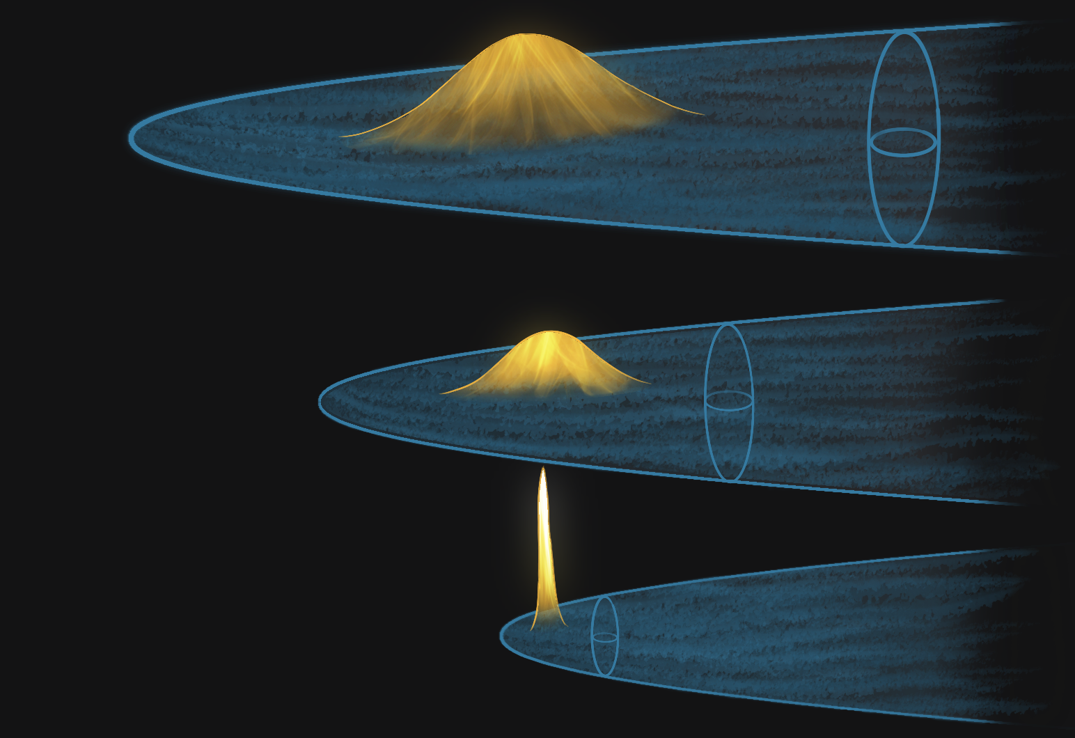
Figure 1: A Ricci flow with a conjugate heat flow

Introduction

The Ricci flow is one of the most important topics in differential geometry, and a central focus of modern geometric analysis. In this paper, we give an illustrated introduction to the Ricci flow for a general audience. In particular, we do not assume any background in differential geometry or differential topology, only that the reader has taken multivariate calculus. For those who are familiar with geometric analysis, we have provided additional details in the footnotes. However, these notes are not necessary to follow the main discussion, so can be ignored on an initial reading.

A short history of the Poincaré conjecture

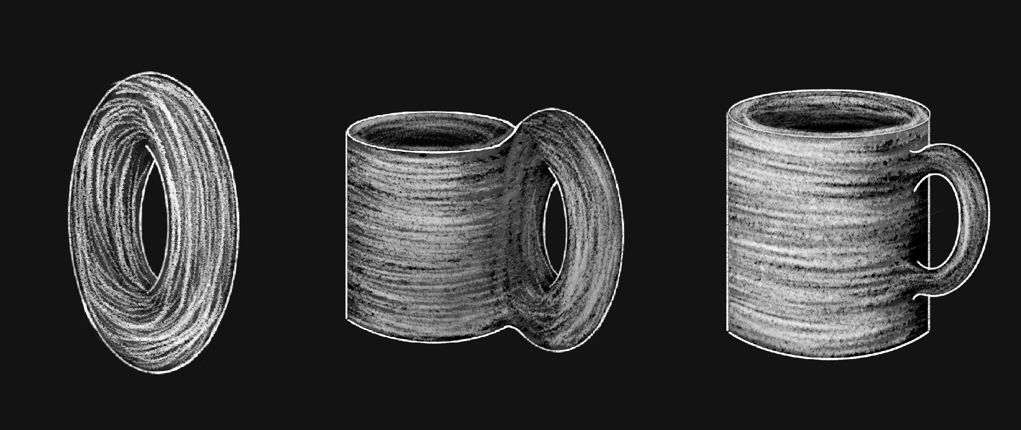
Figure 2: A donut is topologically the same as a coffee mug

The Ricci flow is most famous for its role in the proof of the Poincaré conjecture, so we start our discussion with a historical account of the Poincaré conjecture and some related problems in topology.

In 1905, Henri Poincaré published the seminal paper Analysis Situs [Poi95], which laid the foundations for what is known today as topology. Roughly speaking, topology studies “rubber-sheet geometry,” where spaces are allowed to bend and stretch without tearing. Warping a space will change distances, areas, etc. so the properties studied in topology are quite different from those in traditional geometry. However, one central focus is to find features which do not change when a space is deformed continuously.

While studying this topic, Poincaré conjectured that the three-sphere is the only compact simply-connected three-dimensional manifold. To explain the meaning of this conjecture, it is helpful to first consider the corresponding result for two-dimensional surfaces, which is a special case of the uniformization theorem.

The uniformization theorem

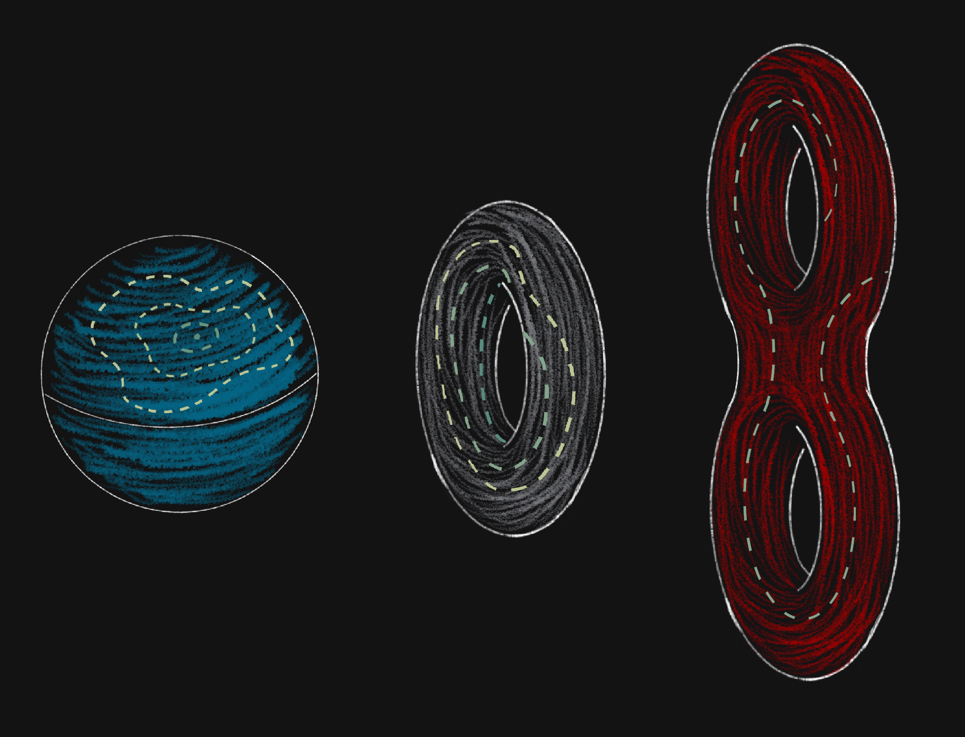
Figure 3: Three surfaces and some loops on them

The uniformization theorem is a celebrated result which classifies the possible geometries on a two-dimensional surface [Poi08]. It states any surface can be deformed into one of three special types of geometries, depending on the number of holes that it has. Surfaces without any holes can be deformed into a round sphere. A surface with one hole (i.e., a donut) can be made into a flat space and any surface with more than one hole admits a hyperbolic geometry.

At first, it might be somewhat hard to visualize the latter two types of geometries. The reason for this is that when we think of surfaces, it is natural to visualize them as living in three-dimensional Euclidean space. However, there is no way to put a flat donut or a hyperbolic surface in $\mathbb{R}^{3}$. To get around this roadblock, we must consider the intrinsic geometry of a surface, without assuming that it lies in some ambient Euclidean space. This can be a major conceptual challenge, but there is an intuitive way to visualize a flat donut using a classic arcade game.

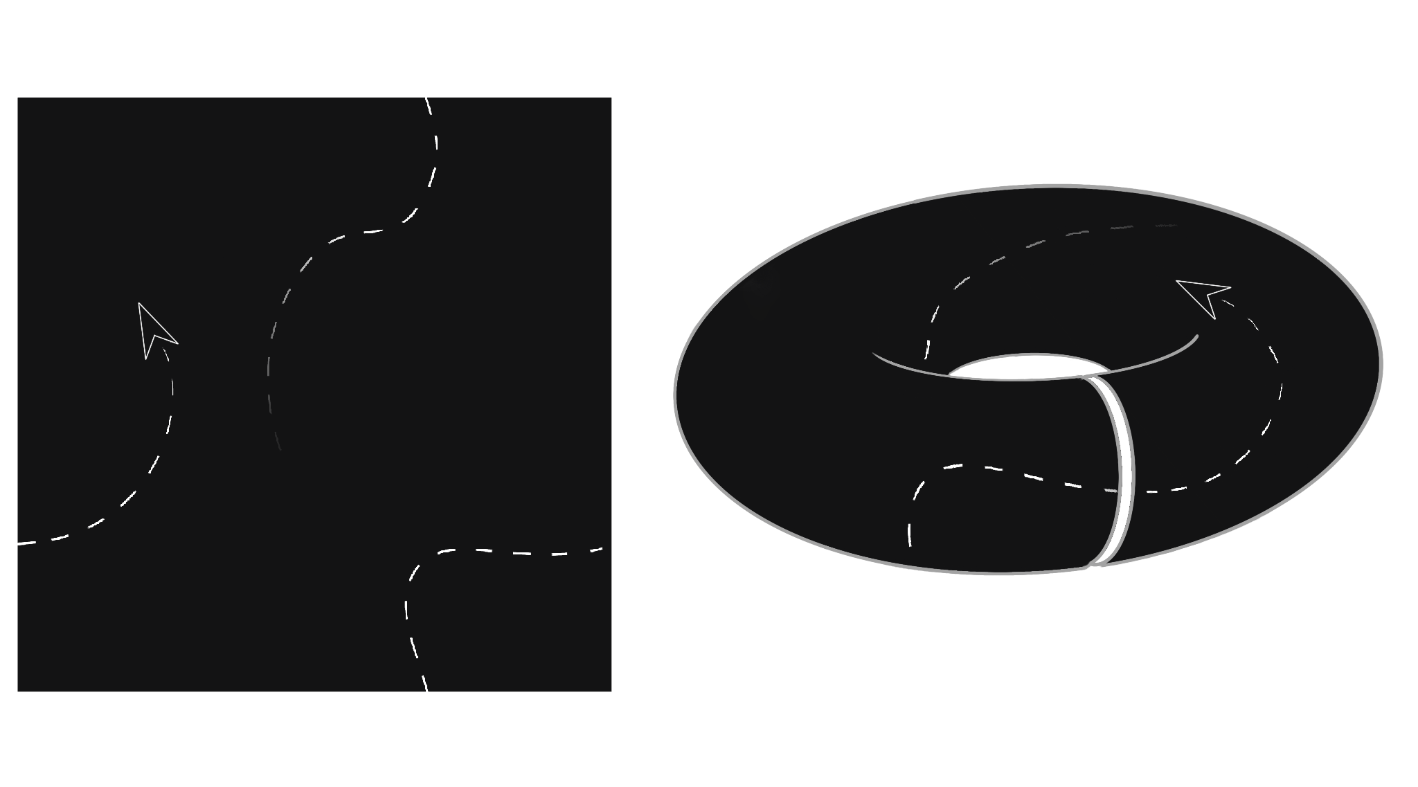
Figure 4: Asteroids on a donut

In the game Asteroids, the player pilots a ship through an asteroid field on the screen, but there is a catch. When the ship flies across the right edge of the screen, it ends up on the left side of screen and when it flies across the top, it ends up at the bottom. It is a worthwhile exercise to show that a space like this is topologically equivalent to a standard donut.

It turns out that there are flat donuts in four-dimensional Euclidean space. Furthermore, there is a very deep theorem by John Nash which states that any possible geometry on a surface can be realized if we consider the surface as living in 51-dimensional Euclidean space [Nas56].

The Poincaré conjecture

The uniformization conjecture has a straightforward, but very important, corollary relating the topology of a surface and the behavior of loops on it. As shown in Figure 5, if we consider a surface with a positive number of holes and draw a loop around the hole, it is not possible to shrink the loop to a point without cutting it or leaving the surface.

As a result, one consequence of the uniformization theorem is that if we are given a surface where every loop drawn in it can be shrunk down continuously to a point, then the space is topologically equivalent to a sphere. Spaces where every loop can be contracted to a point are said to be simply-connected, so another way to state this is that any simply-connected surface is topologically equivalent to a sphere. The Poincaré conjecture is the three-dimensional version of this statement. In other words, if we are given a closed three-dimensional space which is bounded and simply-connected, then the space is topologically equivalent to a three-dimensional sphere.

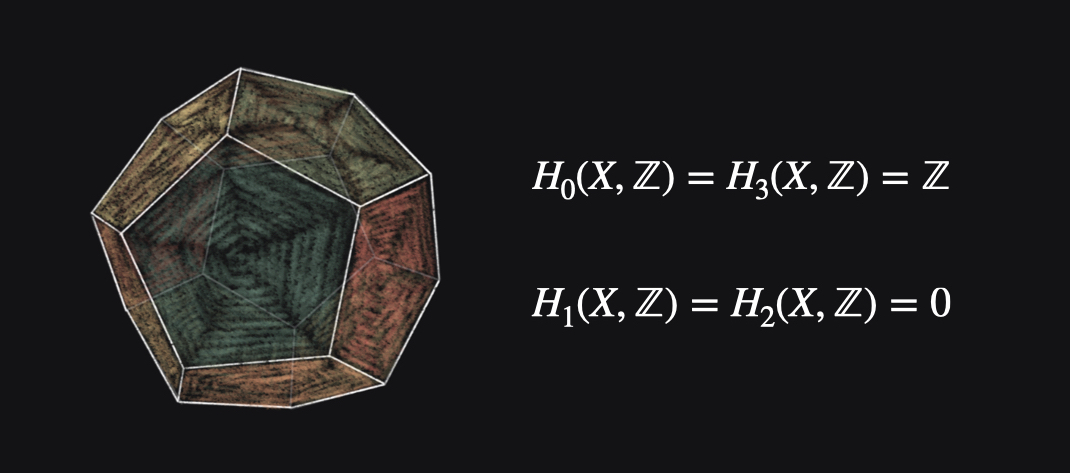
Figure 5: A counter-example to an early version of the Poincaré conjecture

This conjecture (and its higher dimensional analogues) motivated much of the early work in topology. The three-dimensional case in particular proved itself to be extremely subtle and intractable problem (see [Sta16] for some idea of why this is the case). It attracted the attention of many leading mathematicians who developed various tools in their attempts to solve it. As a result of all these efforts, by the 1980s the Poincaré conjecture was settled in all dimensions except for three. However, Poincaré’s original conjecture appeared to be outside the reach of the standard tools of low-dimensional topology, and it seemed that a new approach would be needed to solve it.

The Geometrization Conjecture

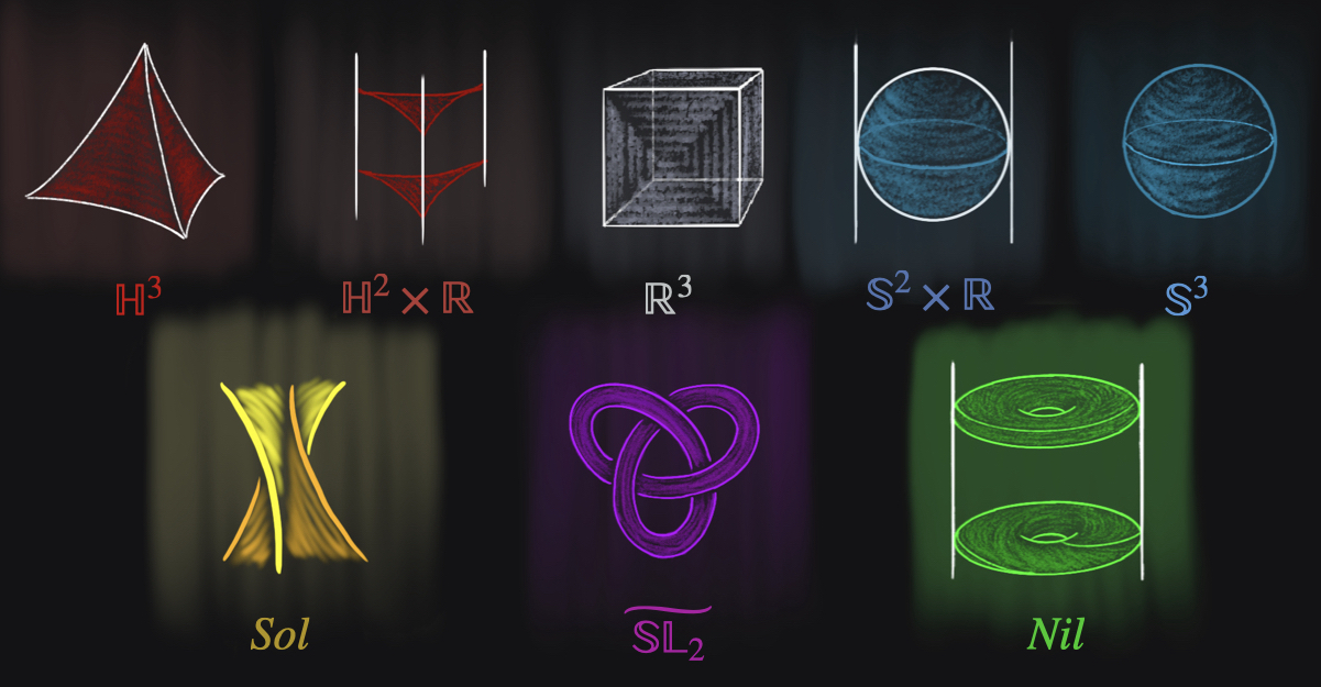
Figure 6: Thurston’s Eight Geometries

In the mid-1970s, William Thurston began a line of work to understand the geometry of three-dimensional spaces, with an emphasis on those with hyperbolic geometry. Building from this work, he proposed a classification for the possible geometries of three-dimensional spaces similar to how the uniformization theorem classifies the geometry of two-dimensional surfaces. More precisely, he found eight canonical three-dimensional geometries and conjectured that given any three-dimensional space, there was a natural way to cut it into pieces which admit one of the geometries. Thurston was able to prove this conjecture for a fairly broad class of spaces and was awarded the Fields Medal in 1982 for this work. His conjecture, known as Thurston’s Geometrization conjecture, implied the Poincaré conjecture and gave a new avenue to attack Poincaré’s question.

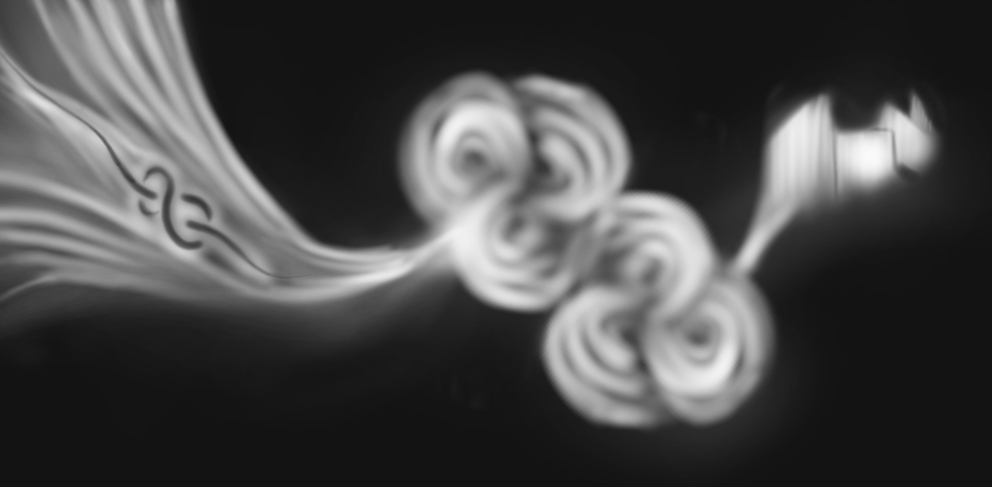
Figure 7: A space formed from three different geometries…

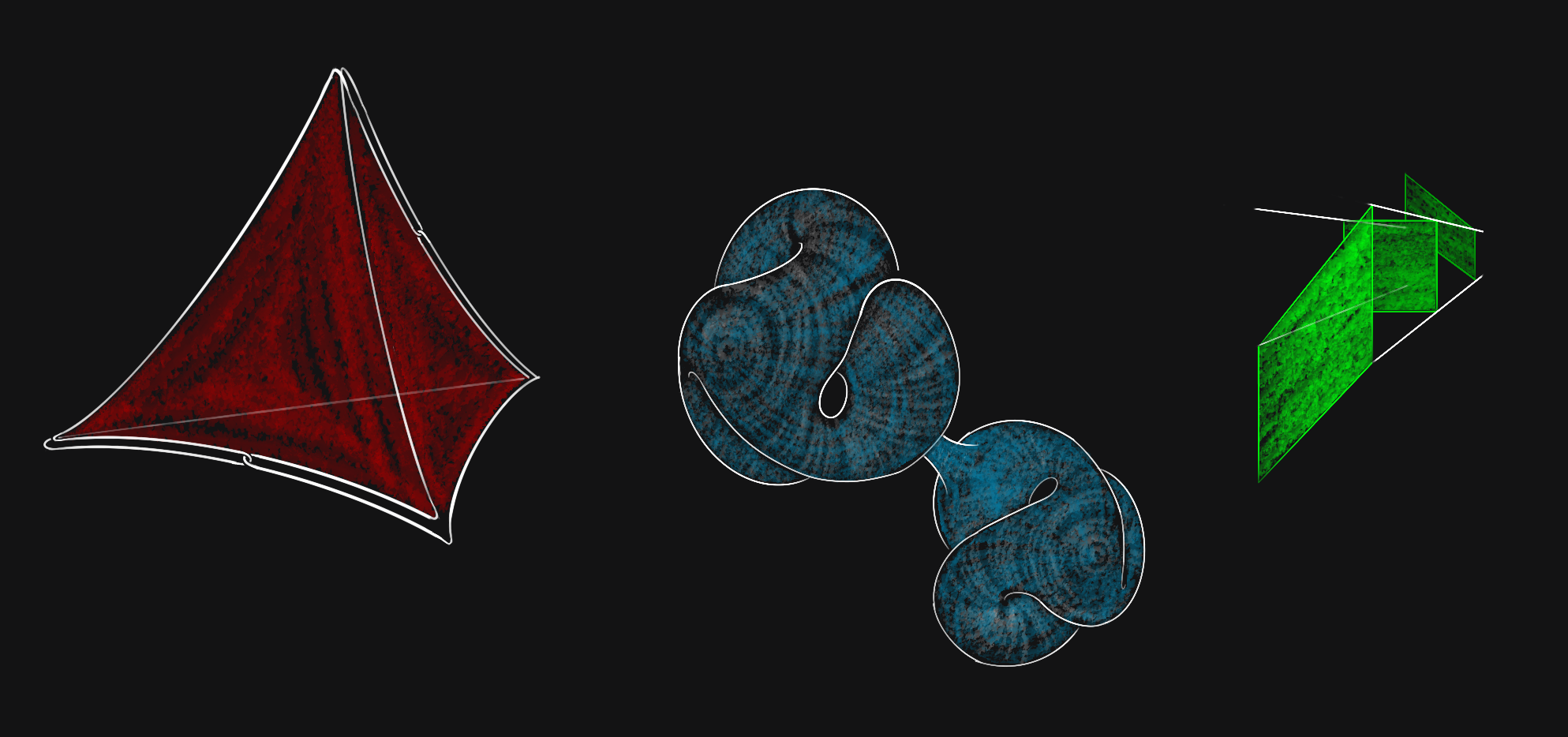
Figure 8: And its geometric decomposition

The Ricci flow

Around this time, Richard Hamilton proposed an ambitious program to attack both of the Geometrization and the Poincaré conjectures [Ham82]. He had been studying work by James Eells and Joseph Sampson [ES64], which used ideas about heat flows to find harmonic maps and thought it might be possible to use a similar approach for these problems. He defined an evolution equation, known as the Ricci flow, which would deform the shape of a space and hopefully allow its curvature to dissipate throughout the space. If the space was simply connected, he hoped the geometry would evolve to that of a round sphere, which would establish the result.

Hamilton and others were able to make partial progress towards this goal. In particular, Hamilton showed that starting with a simply connected three-dimensional space whose Ricci curvature is positive, it would indeed evolve to a round sphere. This was a weaker version of the Poincaré conjecture, but a major proof a concept for the power of the Ricci flow. Furthermore, he was nearly able to find a new proof of the uniformization theorem using Ricci flow. Although the Ricci flow was a promising approach to the Poincaré conjecture, the flow would encounter singularities, which are times where the space would either collapse to a point or violently rip itself apart. Hamilton understood the cases when the space would shrink to a point, but was was not able to control the geometry in the latter case, and this presented a fundamental obstacle to finishing the proof.

Figure 9: The Ricci flow approaching a singularity

Perelman’s breakthrough

In 2000, the Clay Millenium institute listed seven major open problems in mathematics and provided a $1,000,000 prize for a solution to any one of them. The Poincaré conjecture was chosen as one of the problems and despite the best efforts of many mathematicians to solve it, no one expected to see a solution in the near future.

However, just two years later, Grigori Perelman posted a preprint to the arXiv [Per02] with several major breakthroughs in the Ricci flow. In particular, he showed that by coupling the Ricci flow with a heat equation running in reverse, there is a non-decreasing quantity (which corresponds to the Fisher information of the heat distribution) which can be used to control the geometry of its solutions. Perelman claimed that this idea could be used to solve both the Poincaré and Geometrization conjectures, and gave a short sketch of how to do this. This paper took the geometry community by storm, and the experts began to study it to understand what Perelman had found.

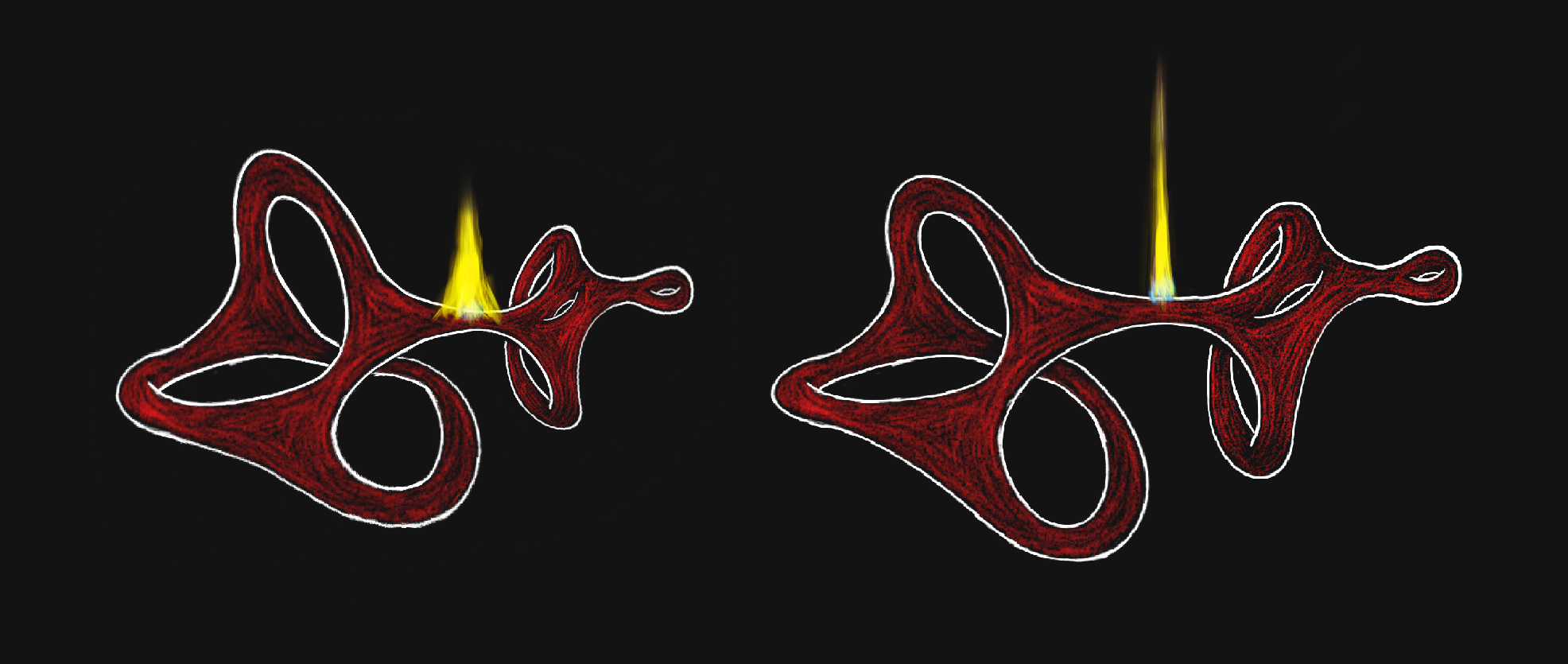
Figure 10: An evolving surface with a backwards heat flow

Over the eight months, two more preprints [Per03b, Per03a] followed the first and provided more details. In particular, Perelman combined the ideas from the first paper with a geometric process known as surgery to excise regions of space when they started to tear apart and replace them with pieces with better behavior. By combining the Ricci flow with surgery, Perelman was able to show that any simply-connected three-dimensional space would converge to a round sphere (or possibly a connected sum of several round spheres), and thus is topologically equivalent to the standard sphere. For more general three-dimensional spaces, he proved that after a large amount of time, Ricci flow with surgery would decompose the space into several pieces whose geometric structure was well understood. This established both the Poincaré conjecture as well as the Geometrization Conjecture.

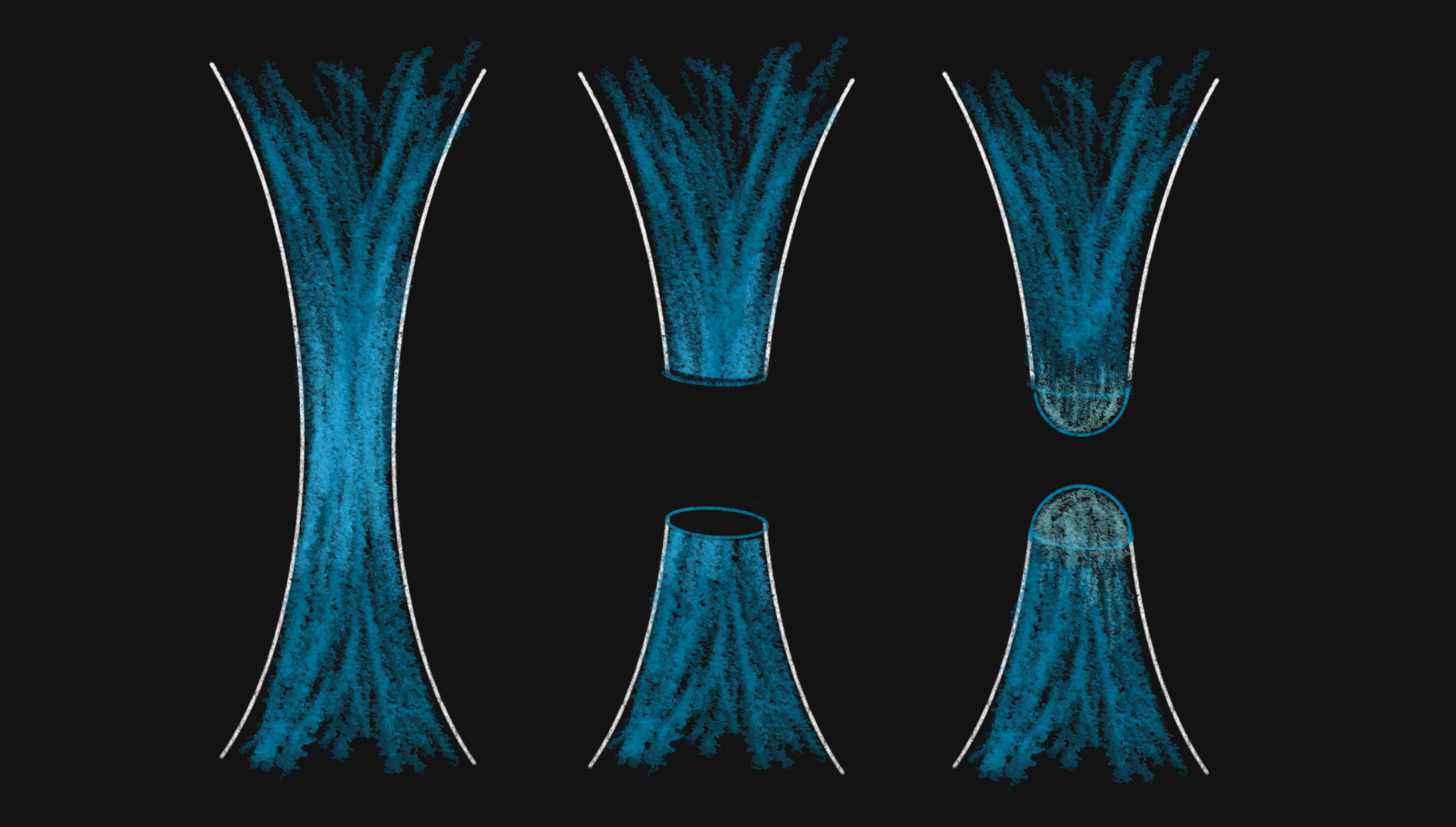
Figure 11: Using surgery to tame singularities

Perelman had worked for nearly a decade in relative isolation, and his proof was the crowning achievement in a long line of work stretching back hundreds of years. The result sparked an enormous amount of interest in geometric analysis and the Ricci flow in particular. However, it took several years (and an authorship scandal) for the mathematical community to accept the work as correct. In 2006, Perelman was awarded a Fields medal for his work, but declined the award and later turned down the Millenium Prize, as well. He has since withdrawn from mathematics.

What is the Ricci flow?

The goal of this chapter is to provide a working definition for the Ricci flow with some intuition for its behavior. Heuristically, the Ricci flow is a “heat flow of curvature” and we will try to explain what this means. To do so, we have divided this chapter into four sections.

• The heat equation and its behavior 14

• The curvature of space 21

• The Ricci flow as a geometric heat flow 28

• Differences between Ricci flow and the standard heat equation 31

The Heat Equation

The heat equation models how the temperature of a region changes in time. More precisely, we consider a function $u(\mathbf{x},t)$ which returns the temperature of a point $\mathbf{x}\in\mathbb{R}^{n}$ at a time $t$. Ignoring what happens at the boundary, we say that the function $u(\mathbf{x},t)$ solves the heat equation if it satisfies

$$\frac{\partial u(\mathbf{x},t)}{\partial t}=\Delta u(\mathbf{x},t).$$ (1)

This equation was introduced by Joseph Fourier in 1822, and played a foundational role in the development of Fourier analysis. We will not provide a physical derivation for why heat distributions tend to obey this equation, but instead try to understand the behavior of its solutions.

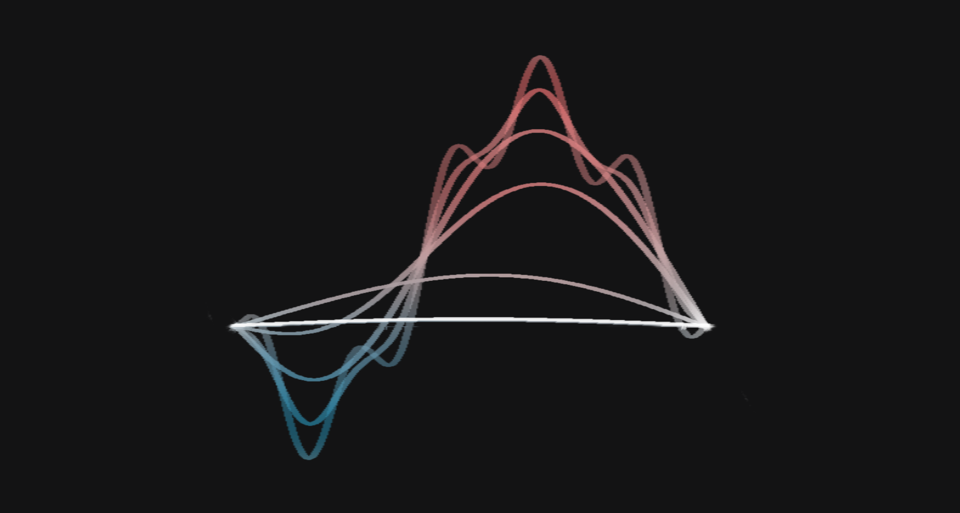
Figure 12: A heat distribution flowing to equilibrium

The Laplacian

Before trying to understand the behavior of solutions to Equation 1, let us first try to understand each of its terms. The left hand side of Equation 1 is the partial derivative of $u$ with respect to $t$, which describes how the temperature at a point $\mathbf{x}$ evolves as time goes by. Therefore, we must understand the term $\Delta u$, which is the Laplacian of $u$. In vector calculus, this is often defined in the following way:

$$\Delta u=\textrm{div}(\textrm{\,grad }u).$$

However, there are several other perspectives on the Laplacian that will tie in more naturally to Ricci flow. One useful interpretation of the Laplacian is to consider the (three-dimensional) Hessian matrix

$$\operatorname{Hess}(u)=\begin{bmatrix}\frac{\partial^{2}}{\partial x^{2}}u&\frac{\partial}{\partial x}\frac{\partial}{\partial y}u&\frac{\partial}{\partial x}\frac{\partial}{\partial z}u\\ \frac{\partial}{\partial y}\frac{\partial}{\partial x}u&\frac{\partial^{2}}{\partial y^{2}}u&\frac{\partial}{\partial y}\frac{\partial}{\partial z}u\\ \frac{\partial}{\partial z}\frac{\partial}{\partial x}u&\frac{\partial}{\partial z}\frac{\partial}{\partial y}u&\frac{\partial^{2}}{\partial z^{2}}u\end{bmatrix}$$

and note that the Laplacian is the trace of this matrix:

$$\Delta u=\frac{\partial^{2}}{\partial x^{2}}u+\frac{\partial^{2}}{\partial y^{2}}u+\frac{\partial^{2}}{\partial z^{2}}u.$$

Later on, we will see that the Ricci curvature is the trace of the Riemann curvature tensor, so this identity makes the connection between the Ricci curvature and the Laplacian fairly natural.

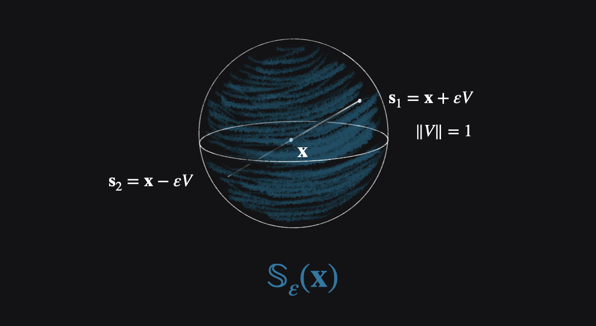
Figure 13: The Laplacian as an integral

In order to define the Ricci flow using the minimal amount of Riemannian geometry, there is a third perspective on the Laplacian that is even more useful. We consider a point $\mathbf{x}$ and a small sphere of radius $\varepsilon$ around $\mathbf{x}$, which we denote $\mathbb{S}_{\varepsilon}(\mathbf{x})$. One can show that the Laplacian is proportional to the difference between $f(\mathbf{x})$ and the average value of $f$ on $\mathbb{S}_{\varepsilon}(\mathbf{x})$:

$$\Delta f(\mathbf{x})=\lim_{\varepsilon\rightarrow 0+}\frac{2n}{\varepsilon^{2}}\frac{1}{\omega\left(\mathbb{S}_{\varepsilon}\right)}\int_{\mathbb{S}_{\varepsilon}(\mathbf{x})}(f(\mathbf{s})-f(\mathbf{x}))\,\mathrm{d}\omega(\mathbf{s}).$$ (2)

Here, $\omega\left(\mathbb{S}_{\varepsilon}\right)$ is the surface area of a sphere of radius $\varepsilon$ in Euclidean $n$-space, which is given explicitly by

$$\omega(\mathbb{S}_{\varepsilon})=\frac{2\pi^{\frac{n}{2}}}{\Gamma\left(\frac{n}{2}\right)}\varepsilon^{n-1}.$$

From this we can see that $\Delta u$ is the average of second derivatives, which is a perspective that will help us understand Ricci curvature. It is worth convincing yourself that the right-hand side of (2) really does have something to do with second derivatives.

Convergence to equilibrium

One hallmark of the heat equation is that its solutions tend to converge to an equilibrium. That is to say, given a function $u(\mathbf{x},t)$ which solves the heat equation, we expect that

$$\lim_{t\to\infty}u(\mathbf{x},t)=C$$

where $C$ is a constant which is independent of the point. Intuitively, if we have a warm cup of coffee outside in a cold day, this states that the heat from the coffee will dissipate into the air and the temperature will converge to that of the outside environment.

There are various ways to make this idea into a precise mathematical statement, and we will mention two that are relevant for understanding the Ricci flow.

The maximum principle

One of the most fundamental tools that one has for studying heat equations is the maximum principle. To give a simple illustration of this principle, we will show that the hot spots of $u(\mathbf{x},t)$ tend to cool down while the cold spots tend to warm up. To do so, we suppose the temperature $u$ is maximized at the point $\mathbf{x}_{0}$ (in the interior of the domain) at some time $t$. Then, since $u(\mathbf{x}_{0},t)$ is maximized, the second derivative test implies that the Hessian of $u$ at $\mathbf{x}_{0}$ must be non-positive definite (i.e., have all non-positive eigenvalues). This implies that $\Delta u(\mathbf{x}_{0},t)$ must also be non-positive. The heat equation then tells us that

$$\frac{\partial u(\mathbf{x}_{0},t)}{\partial t}\leq 0,$$

which is to say that the temperature at $\mathbf{x}_{0}$ is decreasing. If we consider the coldest points, the same argument shows that they warm up under the heat flow.

This type of argument, where one considers a point which maximizes some function and applies the second derivative test (or a more sophisticated version of it) is endlessly useful, and plays an essential role in the analysis of heat-type equations. For example, one can use this argument to prove the Li-Yau estimate [LY86], which states that positive solutions to the heat equation on a space with non-negative Ricci curvature satisfies the inequality

$$\Delta\ln u(\mathbf{x},t)\geq-\frac{n}{t}.$$

This particular estimate plays a fundamental role in geometric analysis, including in the study of the Ricci flow.

Entropy and energy

Another fundamental tool for heat-type equations is to find quantities like energy or entropy which either increase or decrease along the flow. By doing so, one can better understand the behavior of the heat equation.

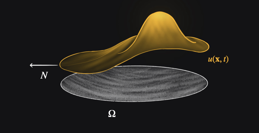
Figure 14: A perfectly insulated domain

To show this idea in practice, we consider the heat equation on a smooth bounded domain $\Omega$ and assume that the domain is perfectly insulated from its surroundings. From a mathematical perspective, this assumption is equivalent to requiring that the temperature at the boundary of the domain satisfies

$$\nabla_{N}u(\mathbf{x},t)=0$$

where $N$ is the outer normal vector, which is known as Neumann boundary conditions.

We then consider the quantity

$$E(t)=\int_{\Omega}u(\mathbf{x},t)^{2}\,d\mathbf{x},$$ (3)

which is often called the energy. However, the name should not be taken too literally because it doesn’t have a direct physical interpretation. Intuitively, it measures how concentrated the heat distribution is. In other words, if $u(\mathbf{x},t)$ is very large in some region $\mathbf{x}$, $E(t)$ will also be large. On the other hand, if the distribution is very diffuse, $E(t)$ will be much smaller. We can compute how $E(t)$ evolves in time as follows.

$$\frac{dE}{dt} = \int_{\Omega}\frac{\partial}{\partial t}u(\mathbf{x},t)^{2}\,d\mathbf{x}$$ (4)

$$= \int_{\Omega}2\left(\Delta u(\mathbf{x},t)\right)\cdot u(\mathbf{x},t)\,d\mathbf{x}.$$ (5)

Using integration by parts and the generalized Stokes’ theorem, it is possible to simplify this expression.

$$\frac{dE}{dt} = -\int_{\Omega}2\|\nabla u(\mathbf{x},t)\|^{2}\,d\mathbf{x}+\int_{\partial\Omega}2u(\mathbf{x},t)\left\langle\nabla u(\mathbf{x},t),N(\mathbf{x})\right\rangle\,d\mathbf{x}.$$ (6)

However, the boundary conditions implies that the second term vanishes.

$$\frac{dE}{dt}=-\int_{\Omega}2\|\nabla u(\mathbf{x},t)\|^{2}\,d\mathbf{x}<0.$$

As such, the energy decreases along the flow, which shows that the heat distribution tends to spread out through space. With a bit more effort, it is also possible to show that this quantity is convex.

Another quantity that we can consider is

$$S=-\int_{\Omega}u(\mathbf{x},t)\ln\left(u(\mathbf{x},t)\right)\,d\mathbf{x},$$

which is better known as the entropy. The entropy is a measure of how disordered a configuration is. More precisely, it is the amount of information (measured in nats) that the heat distribution contains relative to the equilibrium state. However, entropy is a notoriously tricky concept to conceptualize, so for our purposes we can simply define it using the integral above. We can use the same idea from before to calculate the evolution of $S$. Doing so, we find the following:

$$\frac{dS}{dt} = \int_{\Omega}\frac{\|\nabla u\|^{2}}{u}\,d\mathbf{x}>0$$ (7)

The quantity on the right hand side of this equation is known as the Fisher information, and is positive. As such, Equation 7 is a mathematical version of the second law of thermodynamics, which states that a closed system tends to go from an orderly configuration to a disordered state. These types of quantities play a central role in the Ricci flow and one of Perelman’s most important breakthroughs was to find a version of “entropy” for the Ricci flow.

Curvature

In order to discuss the Ricci flow, it is first necessary to discuss the notion of curvature. Unfortunately, rigorously defining curvature requires some background knowledge in Riemannian geometry and a more in-depth discussion of extrinsic versus intrinsic geometry, which are both outside the scope of this introduction. As such, in this section we will provide an intuitive notion of curvature, without trying to be overly precise.

Sectional curvature

It is not immediately obvious what curvature is, especially from an intrinsic perspective where the space of interest does not live in some ambient Euclidean space. However, one useful bit of intuition is that Euclidean space is flat, without any bumps or valleys. As such, one way to formalize the notion of curvature is to compare the geometry of a given space with that of Euclidean space. To do so, the simplest approach is to consider triangles.

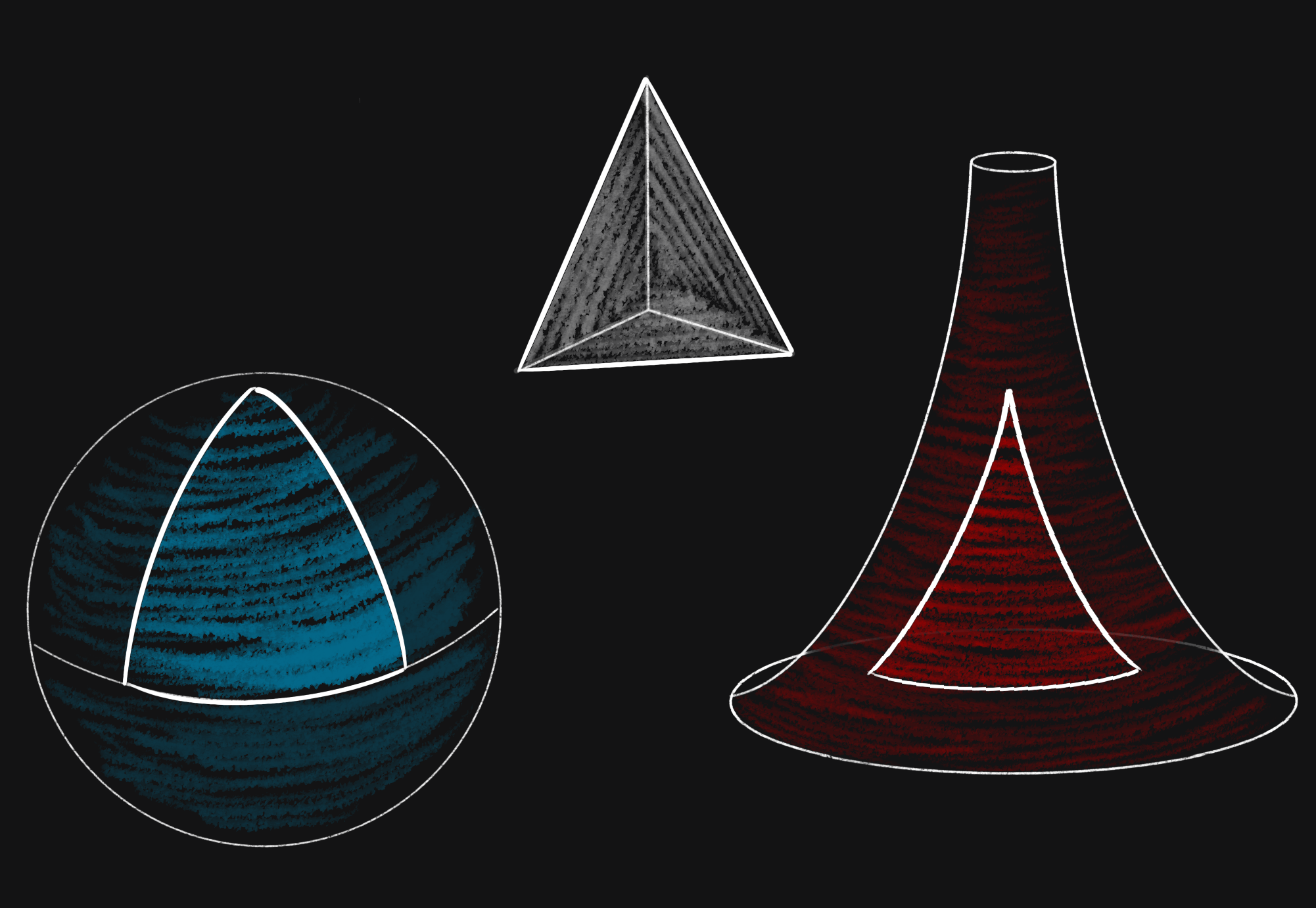
Figure 15: Triangles in spherical, flat and hyperbolic space

As can be seen in Figure 15, triangles on a sphere appear “fatter” than triangles in flat space. There are a few ways to make this precise. For instance, we can consider the sum of the angles of a spherical triangle. It turns out the sum is greater than $\pi$, and actually depends on the area of the triangle. Apart from the angles, we can also see from the picture that the sides of a spherical triangle seem to bow away from the other sides. This bowing occurs in any space of positive curvature, and is one of the characteristic features of positive sectional curvature. To understand this, it helps to picture the sides as turning towards each other, which is why they appear to bow outward. Here, the meaning of the word “turning” is somewhat imprecise, but hopefully the picture makes it clear what we mean.

Before we use this idea to discuss curvature, it is worthwhile to note that round spheres are quite special, in that every point looks like every other point. However, the earth is not exactly a sphere; the geometry of Mount Everest looks very different from that of the Great Plains. This will be true for most of the spaces we are interested in, so we want some way to define curvature on spaces which are not so symmetric. To do so, instead of using a giant triangle as we did on the sphere, we use very small ones.

To do this, we consider a point in our space and two tangent vectors $X$ and $Y$. Then we consider a triangle which has one vertex at $p$ and which has two sides of length $\varepsilon$ in the directions of $X$ and $Y$. We will not be too precise about what it means to make a triangle where the sides “head in a direction,” because it takes some work to define. On the sphere, we saw that the triangle will turned in on itself as a result of the positive curvature. With this in mind, we consider the length of the third edge of the triangle, which we denote $L(\varepsilon)$.

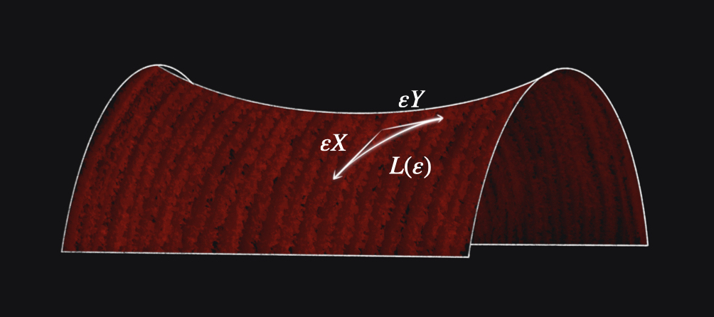
Figure 16: A heuristic diagram for $L(\varepsilon)$

The curvature will be positive whenever $L(\varepsilon)$ is smaller than it would be for a corresponding triangle in Euclidean space and negative if $L(\varepsilon)$ is greater than a triangle in Euclidean space. To make this idea more formal, we consider the Taylor polynomial of $L(\varepsilon)$ in terms of $\varepsilon$. Doing so, we find the following:

$$L(\varepsilon)=\varepsilon\|X-Y\|\left(1-\frac{1}{12}K(X,Y)(1+\langle X,Y\rangle)\varepsilon^{2}\right)+O\left(\varepsilon^{4}\right)$$ (8)

In this expression, $K(X,Y)$ is defined to be the sectional curvature of the tangent plane spanned by $X$ and $Y$. Note that in flat space, $K(X,Y)\equiv 0$ so this matches with our intuition. On the other hand, the unit sphere has constant positive sectional curvature (i.e., $K(X,Y)\equiv 1$). Since $K(X,Y)$ is positive, the third side of the triangle will be shorter than the corresponding side in flat space. Conversely, whenever the sectional curvature is negative, the third side of the triangle will be longer than that of the corresponding Euclidean triangle.

Ricci curvature

While the sectional curvature contains all of the curvature information about a space, it is a very complicated object. The Ricci curvature is a coarser invariant than the sectional curvature, but conveys important geometric information that is essential in many applications. To define it, we consider a unit vector $X$ and define the Ricci curvature $\operatorname{Ric}(X,X)$ to be $(n-1)$ times the average of all of the sectional curvatures of tangent planes containing $X$. In other words, the Ricci curvature satisfies the identity

$$\operatorname{Ric}(X,X)=\frac{1}{2}\frac{(n-1)}{\omega\left(\mathbb{S}^{n-2}\right)}\oint_{\|Y\|=1\textrm{ and }X\perp Y}K(X,Y)\,\mathrm{d}\mathbb{S}^{n-2}(Y),$$ (9)

where $\omega\left(\mathbb{S}^{n-2}\right)$ is the surface area of the $(n-2)$-dimensional sphere. Initially, it might seem a bit strange that the vector $X$ appears twice as an argument for the Ricci curvature, but we will just treat this as a convention without going into detail about why this is the case.

Equation (9) gives a concise definition for the Ricci curvature, but does not provide any intuition for what the Ricci curvature actually is. To do so, it is possible to draw a picture for the Ricci curvature which is similar to the one for sectional curvature but uses cones rather than triangles.

We consider a point $p$, a unit vector $X$ at $p$ and take a short segment of length $\varepsilon$ in the $X$ direction. Finally, we put a narrow circular cone with vertex $p$ around the segment (here, the cone being narrow means that the cone angle $\theta$ satisfies $\tan(\theta)=\varepsilon$). We then consider the area of the base of the cone, which we denote $A(\varepsilon)$.

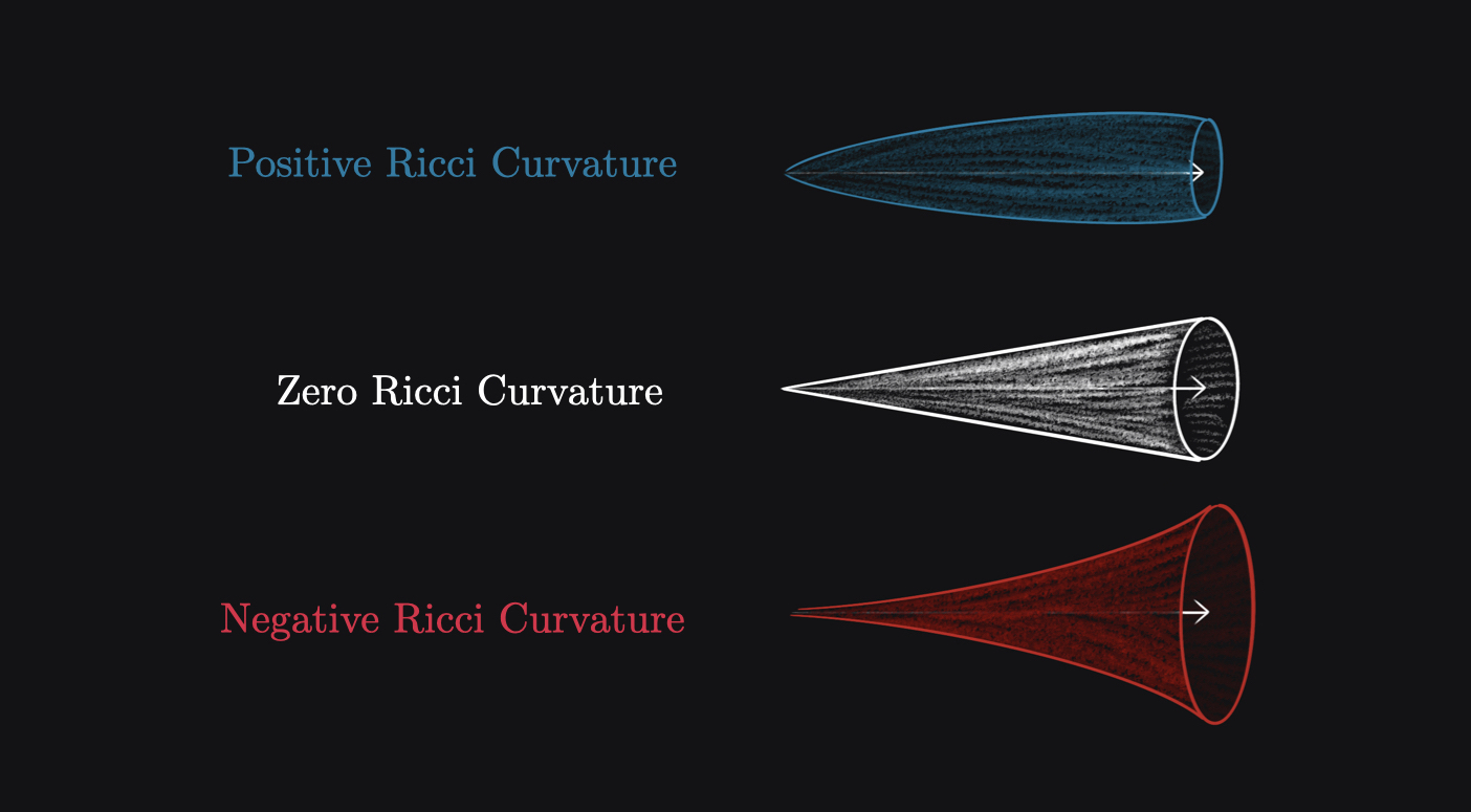
Figure 17: Cones with various Ricci curvatures

When the Ricci curvature is positive, the cone will close in on itself whereas in negatively curved space, the cone will open outward (as shown in Figure 17). In this spirit, when we compute the Taylor expansion of $A(\varepsilon),$ we find the following:

$$A(\varepsilon)=\varepsilon^{2(n-1)}\left(D_{n-1}-C_{n}\operatorname{Ric}(X,X)\varepsilon^{2}\right)+O(\varepsilon^{2n+1}).$$ (10)

Here $D_{n-1}$ is the volume of a unit disk in Euclidean $(n-1)$-space and $C_{n}$ is a complicated, but positive, constant which depends on the dimension. The factor of $\varepsilon^{2(n-1)}$ on the right-hand comes from the fact that the cone is both short and narrow, both of which contribute to the area of the base being small.

The Ricci curvature as a geometric Laplacian

Heuristically, the sectional curvature can be understood as a geometric second derivative. In particular, ignoring the $\varepsilon$ at the front of Equation (8) (which comes from the fact that the associated triangle has very short sides), the sectional curvature appears in the second-order position. With this intuition, comparing Equations (2) and (9) suggests that the Ricci curvature is a sort of geometric Laplacian. Making this heuristic rigorous requires a bit of Riemannian geometry, because the sectional curvature $K(X,Y)$ does not depend linearly on $X$ and $Y$.

We won’t go into too much detail about how to make this idea precise. The basic idea is that the sectional curvature can be used to construct the Riemann curvature tensor, which is comparable to a geometric Hessian. The Ricci curvature is the trace of the Riemann curvature tensor, which gives further credence to its interpretation as a geometric Laplacian.

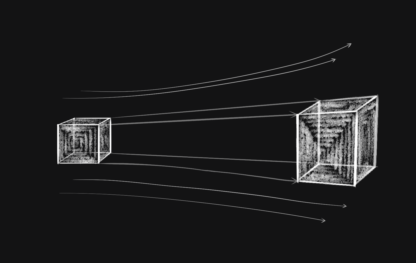
Figure 18: The compression of a fluid flow

There is one other important analogy between the usual Laplacian and the Ricci curvature, which is that they both measure how volumes change. More precisely, given a smooth function $f:\mathbb{R}^{3}\to\mathbb{R}$, we can consider the gradient flow

$$\frac{d}{dt}\gamma(t)=-\nabla f(\gamma),$$

which takes a point and moves in the direction which decreases $f$ the quickest. Doing so, the quantity $\Delta f(\mathbf{x})$ measures how much the volume of a very small cube around $\mathbf{x}$ will change under the flow. In other words, if we consider $\nabla f$ as the current of some fluid, $\Delta f$ measures the compression of the flow. In a similar way, the Ricci curvature determines how volumes of small cubes change as we move from one point to another on a curved space. In other words, it measures how volumes are compressed due to the curvature of the space.

The Ricci Flow

Now that we have discussed the heat equation as well as the notion of Ricci curvature, we can finally talk about the Ricci flow, which can be understood as a “geometric heat equation.” To get started, we will provide an informal geometric explanation.

Definition.

The Ricci flow changes the shape of a space proportional to -2 times the Ricci curvature.

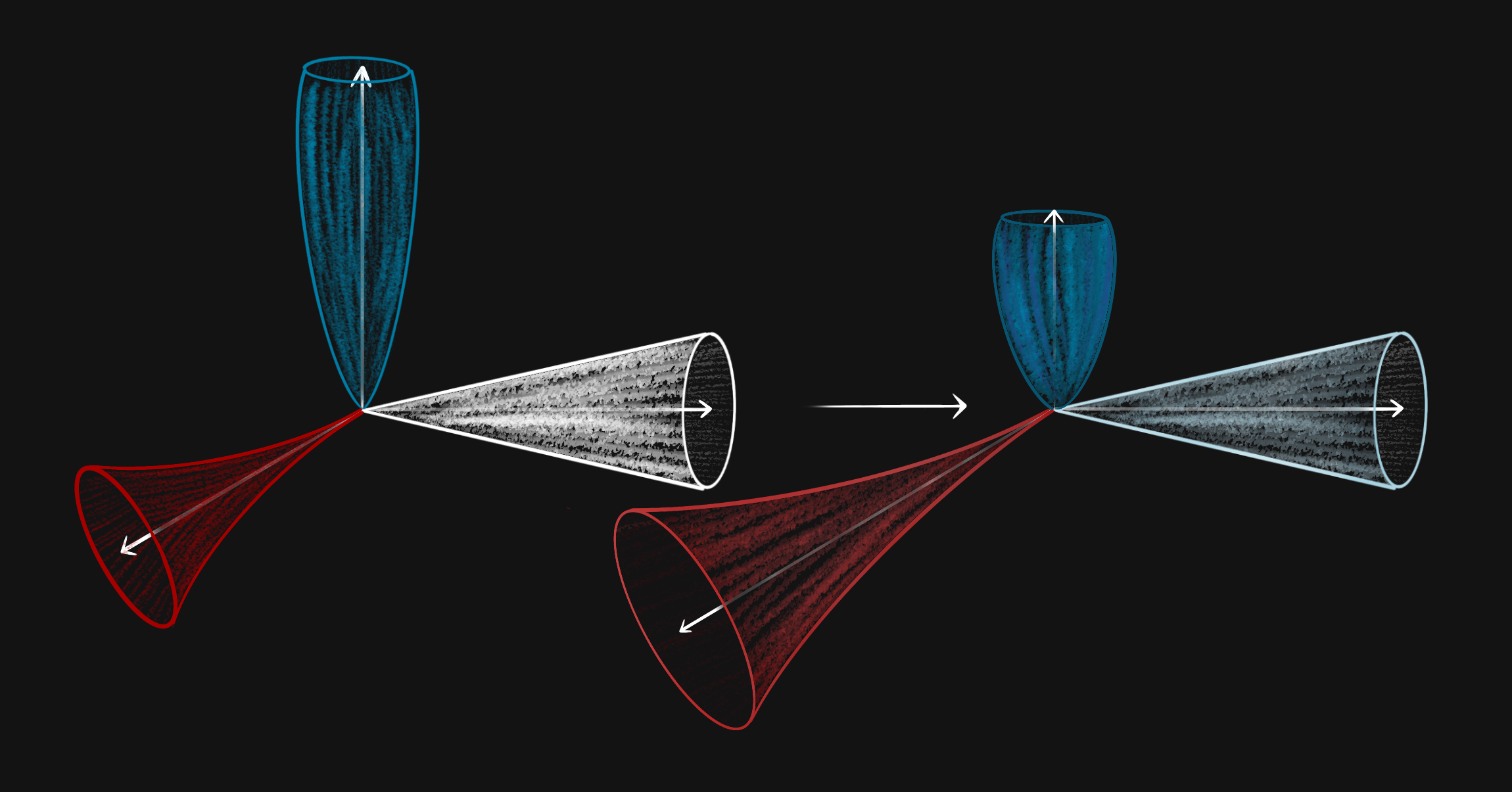
Figure 19: Ricci flow deforming a basis which is initially orthonormal

In other words, directions which have negative Ricci curvature get longer whereas directions with positive Ricci curvature get shorter (as depicted in Figure 45).

In order to define the Ricci flow precisely, we must formalize what the “shape” of a space is. For surfaces in Euclidean space, it is clear enough what this refers to, but it is much more challenging to define the shape intrinsically when it is not lying in some higher dimensional space. To do so, we can use the notion of a Riemannian metric, which is a generalization of the dot product in Euclidean space. In other words, it provides an inner product of two tangent vectors (at the same point) in our space. There is a fundamental theorem in differential geometry that states that this structure fully determines the geometry of the space, and that it is possible to compute the curvature of the space (as well as all the other metric invariants) from this inner product alone. However, the formulas involved are very complicated, so we will just consider the Riemannian metric $g$ as a geometric object that encodes the “shape” of our space. Using the metric, the equation for the Ricci flow becomes

$$\frac{\partial}{\partial t}g=-2\operatorname{Ric}(g).$$ (11)

It is worth spending some time to make sure this is really a sensible formula, since there are several strange properties. The first is that our definition of Ricci curvature required that we input a vector (which we wrote, somewhat bizarrely, as two separate entries). In fact, the Riemannian metric $g$ also requires that we input two vectors, so this is actually part of what makes the Ricci flow work.

The second objection to considering this equation as a heat equation is that right hand side has a factor of $-2$ whereas the heat equation $\frac{\partial u}{\partial t}=\Delta u$ does not. This factor appears because the Ricci curvature should be thought of as the negative of a geometric Laplacian. In other words, the analytic Laplacian and geometric “Laplacian” differ by a sign.

With these objections addressed, there is an apparent parallel between this formula and the heat equation $\frac{\partial u}{\partial t}=\Delta u$. We have tried to justify why it is possible to think of the Ricci curvature tensor as being analogous to a geometric Laplacian, which suggests that the Ricci flow is a heat flow of “shape.” As a demonstration of this fact, it is worthwhile to see an example of the Ricci flow in action, which is depicted in Figure 50. There are also some animations of the flow, which are helpful to understand how it behaves  [Pro]. In both the video and the figure, the surface becomes more spherical as time goes on. In the same way that the heat equation spreads the heat evenly throughout the space, the Ricci flow spreads the curvature evenly throughout the space.

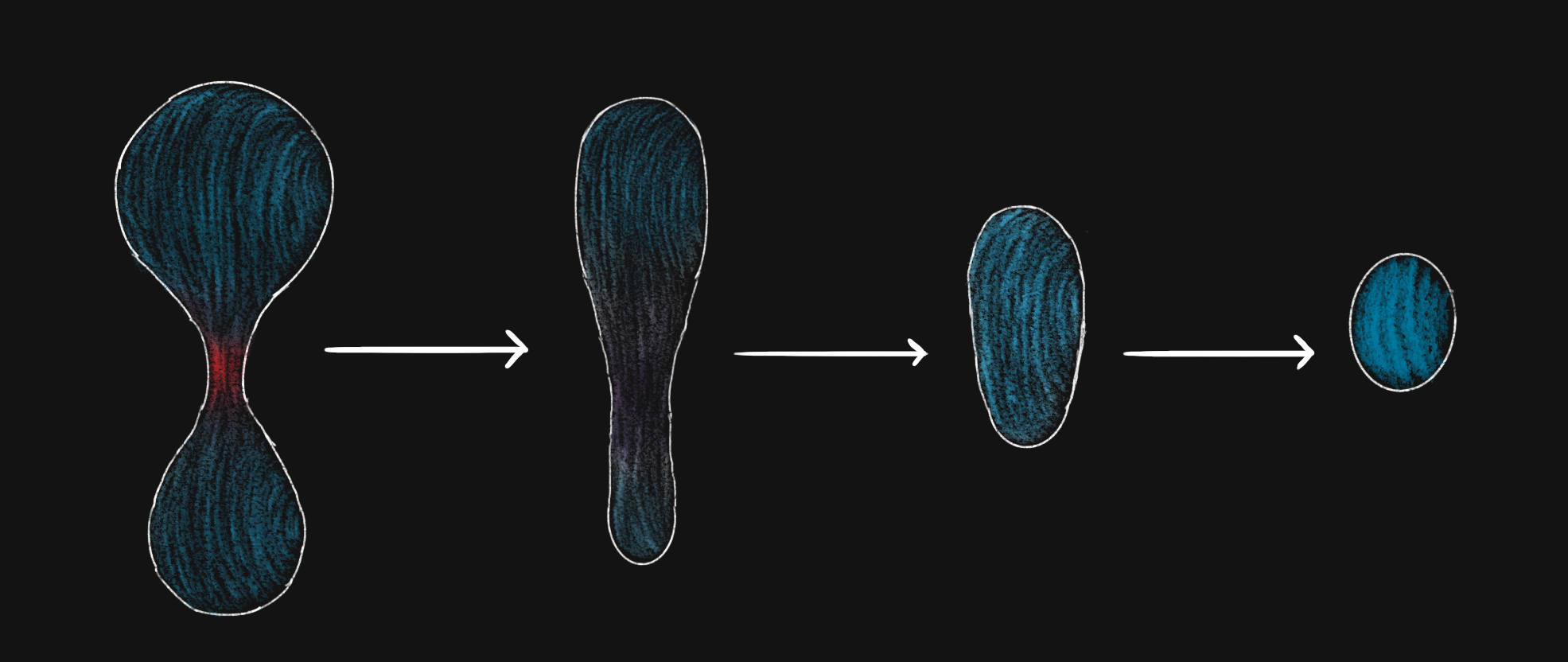
Figure 20: The Ricci flow converging to a round sphere

Distinctions between the Ricci flow and heat equation

From the analogy between the heat equation and the Ricci flow, we might hope that the Ricci flow will smooth out our space and make it more uniform. In reality, the Ricci flow is more complicated than a heat flow, so this hope is too optimistic.

The first important distinction between the heat equation and the Ricci flow is that the latter is non-linear (linear combinations of solutions are no longer solutions) because curvature depends in a non-linear way on the metric. Second, it actually behaves more similarly to the reaction-diffusion equation

$$\frac{\partial}{\partial t}u=\Delta u+u^{2}.$$ (12)

The first term on the right-hand side behaves as a diffusion term that disperses heat throughout the space whereas the second acts a reaction term that concentrates heat at a point. Reaction-diffusion equations can be thought as a tug-of-war between the diffusion process and the reaction process. If diffusion wins, the solution will smooth itself out much like the normal heat equation. If the reaction term wins out, the heat will become more and more intense and can sometimes even become become infinite in a finite amount of time. An example of this is shown in Figure 53, where the solution becomes infinitely large after a short amount of time.

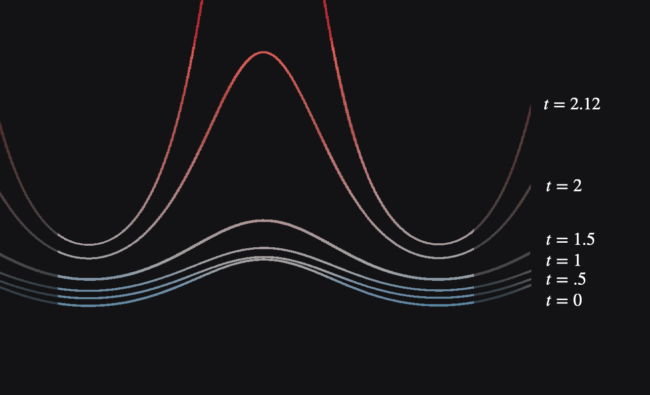
Figure 21: A reaction-diffusion equation going to infinity

When we compute how the Riemann curvature (denoted $R$) of a space changes along Ricci flow, we find the following equation:

$$\frac{\partial}{\partial t}R=\Delta R+R^{2}+R^{\sharp}.$$ (13)

It takes some background in Lie algebra to define the terms on the right-hand side of this formula [Wil13]. However, ignoring the final term on the right hand side, there is a notable similarity between this equation and Equation (12). In particular, sometimes the reaction term wins out and the curvature becomes larger and larger until the shape tears itself apart (or shrinks to a point). However, understanding the formation of singularities is difficult because it is not obvious when they occur or what they look like. One of Perelman’s key contributions was to classify the possible structures of three-dimensional singularities and to show that a singularity known as the “cigar soliton” would not develop.

Figure 22: A Ricci flow becoming singular

Recent progress and future directions

The Ricci flow is an active area of research, both as a tool to prove geometric and topological results and also as a topic of interest in its own right. It would be impossible to give a complete overview of the current state of research, but let us mention a few broad areas of interest.

The long-term behavior and singularity formation of the Ricci flow

The singularity formation and convergence of the Ricci flow is a fascinating and difficult topic. There are many open questions about when singularities occur and what their possible geometries can be. The most famous open problem in this direction is to determine whether the scalar curvature (i.e., the trace of the Ricci curvature) necessarily becomes infinite at a singularity.

There has also been research into the structure of Ricci flows which are allowed to become singular and the singularities that form under “generic” initial conditions. For details on this line of work, we recommend the recent survey articles by Richard Bamler [Bam21] and Simon Brendle [Bre22].

Geometric classification results

Apart from the Poincaré conjecture, the Ricci flow has been used to prove other geometric classification results. To give a few examples, Hamilton used Ricci flow to understand the geometry of three-dimensional spaces with positive Ricci curvature [Ham82] and four-dimensional spaces with positive curvature operator [Ham97]. In 2007, Brendle and Richard Schoen proved the Differentiable Sphere Theorem using the Ricci flow [Bre10] and Brendle recently used it to establish a partial classification of higher-dimensional spaces with positive isotropic curvature [Bre19].

There are also several ongoing programs which use Ricci flow (or some related flow) to attack open problems in geometry.

1. The minimal model program is a central focus of birational geometry, which is a branch of algebraic geometry involving rational functions. Jian Song and Gang Tian proposed using Kähler-Ricci flow (with surgery) to find the minimal models analytically. [ST17].

2. The Ricci flow tends to make the curvature of spaces more positive. As such, it is very useful for studying and classifying spaces with positive curvature. For instance, the Ricci flow may be useful for fully classifying spaces which admit metrics of positive isotropic curvature or whose squared-distance has non-negative MTW tensor (see Chapter 12 of [Vil09] for a definition of this condition).

3. Finally, there are several problems concerning the geometry of four-dimensional spaces which seem amenable to a Ricci flow approach (see Section 5.6 of [Bam21] for some details).

Other geometric flows

The idea of using a heat-type flow to take geometric space and deform it to some canonical configuration predates the Ricci flow, but this approach has exploded in popularity in the four decades since the Ricci flow was first studied. At present, there are many geometric flows studied in the literature: mean curvature flow, harmonic map heat flow, Kähler-Ricci flow, Chern-Ricci flow, pluriclosed flow, anomaly flow, Calabi flow, Yamabe flow…

These flows play a significant role in differential geometry and have many applications, both within pure mathematics and more broadly. There is still much to be said about the behavior of geometric flows, and it is an active and vibrant area of research.

Endnotes

Further reading

Readers who are interested in the Poincaré conjecture may enjoy Donal O’Shea’s book “The Poincaré Conjecture: In Search of the Shape of the Universe,” which is intended for a general audience and gives a detailed history of the problem and its wider role in geometry [O’S08].

This paper discussed the uniformization theorem, but did not describe hyperbolic or spherical geometries in detail. For a basic introduction to this subject, I recommend the book “The Shape of Space” by Jeffrey Weeks. Chapter 6 of Tristan Needham’s book “Visual Complex Analysis” provides an excellent description of the canonical two-dimensional geometries for those who are familiar with complex analysis (or are interested in learning about it) [Nee98]. Thurston’s “The Geometry and Topology of Three-Manifolds” is excellent for learning about the three-dimensional geometries [Thu79].

For readers who are interested in learning differential geometry, I highly recommend Needham’s recent book [Nee21] or John Lee’s trilogy [Lee10, Lee13, Lee18]. For those conversant with differential geometry who are interested in geometric analysis, Schoen and Shing-Tung Yau’s Lectures in Differential Geometry is excellent, although a more challenging read [SY94].

The discussion of curvature in this paper was strongly influenced by the synthetic theory of curvature bounds. I recommend the following paper of Villani for details on this approach [Vil16]. There were two reasons I chose this perspective. First, it makes it possible to discuss the geometric meaning of curvature without needing to first define connections, parallel transport, etc. Second, the proof of the Geometrization conjecture uses Alexandrov geometry, so synthetic curvature plays a crucial role in the analysis of Ricci flow. The primary disadvantage of this approach is that it is practically impossible to use for computations, but this was not such an issue for an informal survey.

In order to study the Ricci flow, a good starting point is Peter Topping’s manuscript “Lectures on Ricci flow” [Top06]. From there, Hamilton’s paper on the formation of singularities is well worth reading [Ham93]. Understanding the full proof of the Poincaré conjecture is a massive undertaking (and the full Geometrization conjecture even more so), but there have been several surveys written and I recommend the following [KL08, MT07]. Furthermore, Danny Calegari recently wrote a chapter on the proof which emphasizes the three-dimensional geometry [Cal20].

Acknowledgements

This project started as lecture notes for a talk at the “What is…?” seminar at Ohio State University in 2015. The seminar was aimed at advanced high school students at the Ross program, who had taken multivariate calculus and linear algebra, but were not expected to know any differential geometry. I would like to thank the organizers for letting me give a talk about a subject well outside the normal purview of the seminar.

Finding ways to discuss the Ricci flow without assuming any background in differential geometry was a challenge, and I relied on the help of several people to find explanations which avoided going into detail about Riemannian geometry or PDEs. In particular, thanks to Kori Khan for her helpful suggestions and to Mizan Khan for his help editing the paper. I would also like to thank Frank Nielsen for some corrections.

Bibliography

- [Bam18] Richard Bamler. Long-time behavior of 3–dimensional Ricci flow: introduction. Geometry & Topology, 22(2):757–774, 2018.
- [Bam21] Richard H Bamler. Recent developments in Ricci flows. Notices of the AMS, 68(9):1486–1498, 2021.
- [BCRW19] Richard H Bamler, Esther Cabezas-Rivas, and Burkhard Wilking. The Ricci flow under almost non-negative curvature conditions. Inventiones mathematicae, 217(1):95–126, 2019.
- [Bre10] Simon Brendle. Ricci flow and the sphere theorem, volume 111. American Mathematical Soc., 2010.
- [Bre19] Simon Brendle. Ricci flow with surgery on manifolds with positive isotropic curvature. Annals of Mathematics, 190(2):465–559, 2019.
- [Bre22] Simon Brendle. Singularity models in the three-dimensional Ricci flow. arXiv preprint math/2201.02522, 2022.
- [Cal20] Danny Calegari. Chapter 6: Ricci flow. 2020.
- [Cho91] Bennett Chow. The Ricci flow on the 2-sphere. Journal of Differential Geometry, 33(2):325–334, 1991.
- [CLT06] Xiuxiong Chen, Peng Lu, and Gang Tian. A note on uniformization of Riemann surfaces by Ricci flow. Proceedings of the American Mathematical Society, pages 3391–3393, 2006.
- [CMST20] Rémi Coulon, Elisabetta A Matsumoto, Henry Segerman, and Steve Trettel. Non-euclidean virtual reality III: Nil. arXiv preprint arXiv:2002.00513, 2020.
- [DeT81] Dennis M DeTurck. Existence of metrics with prescribed Ricci curvature: local theory. Inventiones mathematicae, 65(2):179–207, 1981.
- [ES64] James Eells and Joseph H Sampson. Harmonic mappings of Riemannian manifolds. American journal of mathematics, 86(1):109–160, 1964.
- [Fre82] Michael Hartley Freedman. The topology of four-dimensional manifolds. Journal of Differential Geometry, 17(3):357–453, 1982.
- [Gro86] Mikhael Gromov. Partial differential relations, volume 9. Springer Science & Business Media, 1986.
- [Ham82] Richard S Hamilton. Three-manifolds with positive Ricci curvature. Journal of Differential geometry, 17(2):255–306, 1982.
- [Ham93] Richard Hamilton. The formations of singularities in the Ricci flow. Surveys in differential geometry, 2(1):7–136, 1993.
- [Ham97] Richard S Hamilton. Four-manifolds with positive isotropic curvature. Communications in Analysis and Geometry, 5(1):1–92, 1997.
- [KL08] Bruce Kleiner and John Lott. Notes on Perelman’s papers. Geometry & Topology, 12(5):2587–2855, 2008.
- [KZ20] Gabriel Khan and Fangyang Zheng. Kähler-Ricci flow preserves negative anti-bisectional curvature. arXiv:2011.07181, 2020.
- [Lee10] John Lee. Introduction to Topological Manifolds, volume 202. Springer Science & Business Media, 2010.
- [Lee13] John M Lee. Introduction to Smooth Manifolds. Springer, 2013.
- [Lee18] John M Lee. Introduction to Riemannian Manifolds. Springer, 2018.
- [LY86] Peter Li and Shing Tung Yau. On the parabolic kernel of the Schrödinger operator. Acta Mathematica, 156:153–201, 1986.
- [Mil59] John Milnor. Differentiable structures on spheres. American Journal of Mathematics, 81(4):962–972, 1959.
- [MT07] John W Morgan and Gang Tian. Ricci flow and the Poincaré conjecture, volume 3. American Mathematical Soc., 2007.
- [Nas56] John Nash. The imbedding problem for Riemannian manifolds. Annals of mathematics, pages 20–63, 1956.
- [Nee98] Tristan Needham. Visual Complex Analysis. Oxford University Press, 1998.
- [Nee21] Tristan Needham. Visual Differential Geometry and Forms: A Mathematical Drama in Five Acts. Princeton University Press, 2021.
- [O’S08] Donal O’Shea. The Poincaré conjecture: In search of the shape of the universe. Bloomsbury Publishing USA, 2008.
- [Per02] Grisha Perelman. The entropy formula for the Ricci flow and its geometric applications. arXiv preprint math/0211159, 2002.
- [Per03a] Grisha Perelman. Finite extinction time for the solutions to the Ricci flow on certain three-manifolds. arXiv preprint math/0307245, 2003.
- [Per03b] Grisha Perelman. Ricci flow with surgery on three-manifolds. arXiv preprint math/0303109, 2003.
- [Poi95] Henri Poincaré. Analysis Situs. Gauthier-Villars Paris, France, 1895.
- [Poi08] Henri Poincaré. Sur l’uniformisation des fonctions analytiques. Acta mathematica, 31:1–63, 1908.
- [Pro] Mathifold Project. Ricci flow. Available at https://www.youtube.com/watch?v=siAbBsj9XPk.
- [Šeš05] Nataša Šešum. Curvature tensor under the Ricci flow. American journal of mathematics, 127(6):1315–1324, 2005.
- [Sma62] Stephen Smale. On the structure of manifolds. American Journal of Mathematics, 84(3):387–399, 1962.
- [ST17] Jian Song and Gang Tian. The Kähler–Ricci flow through singularities. Inventiones mathematicae, 207(2):519–595, 2017.
- [Sta16] John Stallings. How not to prove the Poincaré conjecture. In Topology Seminar Wisconsin, 1965.(AM-60), Volume 60, pages 83–88. Princeton University Press, 2016.
- [SY94] Richard M Schoen and Shing-Tung Yau. Lectures on differential geometry, volume 2. International press Cambridge, MA, 1994.
- [Thu79] William P Thurston. The geometry and topology of three-manifolds. Princeton University Princeton, NJ, 1979.
- [Top06] Peter Topping. Lectures on the Ricci flow, volume 325. Cambridge University Press, 2006.
- [Vil09] Cédric Villani. Optimal transport: old and new, volume 338. Springer, 2009.
- [Vil16] Cédric Villani. Synthetic theory of Ricci curvature bounds. Japanese Journal of Mathematics, 11(2):219–263, 2016.
- [Wil13] Burkhard Wilking. A Lie algebraic approach to Ricci flow invariant curvature conditions and Harnack inequalities. Crelle’s Journal, 2013(679):223–247, 2013.