Interface potential and line tension for Bose-Einstein condensate mixtures
near a hard wall

Abstract

Within Gross-Pitaevskii (GP) theory we derive the interface potential $V(\ell)$ which describes the interaction between the interface separating two demixed Bose-condensed gases and an optical hard wall at a distance $\ell$. Previous work revealed that this interaction gives rise to extraordinary wetting and prewetting phenomena. Calculations that explore non-equilibrium properties by using $\ell$ as a constraint provide a thorough explanation for this behavior. We find that at bulk two-phase coexistence, $V(\ell)$ for both complete wetting and partial wetting is monotonic with exponential decay. Remarkably, at the first-order wetting phase transition, $V(\ell)$ is independent of $\ell$. This anomaly explains the infinite continuous degeneracy of the grand potential reported earlier. As a physical application, using $V(\ell)$ we study the three-phase contact line where the interface meets the wall under a contact angle $\theta$. Employing an interface displacement model we calculate the structure of this inhomogeneity and its line tension $\tau$. Contrary to what happens at a usual first-order wetting transition in systems with short-range forces, $\tau$ does not approach a nonzero positive constant for $\theta\rightarrow 0$, but instead approaches zero (from below) in the manner $\tau\propto-\theta$ as would be expected for a critical wetting transition. This hybrid character of $\tau$ is a consequence of the absence of a barrier in $V(\ell)$ at wetting. For a typical $V(\ell)=\mathcal{S}\exp(-\ell/\xi)$, with $\mathcal{S}$ the spreading coefficient, we conjecture that $\tau=-2\,(1-\ln 2)\,\gamma\,\xi\,\sin\theta$ is exact within GP theory, with $\gamma$ the interfacial tension and $0\leq\theta\leq\pi$.

I Introduction

The experimental realization of Bose-Einstein condensation (BEC) in dilute Bose gases, now more than twenty-five years ago, initiated big experimental and theoretical advances in the field of ultracold gases pita . Most interesting in this context is that one gained immediate access to, and extended experimental control of the physics of, very pure quantum systems. For example, by means of Feshbach resonances inouye ; stan ; papp , one is capable of tuning the interactions between the trapped atoms. Furthermore, an evanescent wave surface trap provides one with adjustable particle-wall interactions and permits one to approximate a “hard wall” type of boundary  rychtarik ; perrin .

Uniform (flat-bottom) optical-box traps are now increasingly used to establish homogeneous ultracold gases in different dimensionality  gaunt ; navon . This is particularly interesting from our perspective in this paper because a homogeneous system in semi-infinite geometry is the ideal theoretical setting for studying wetting phenomena. Therefore, results of experiments in flat-bottom traps can be compared straightforwardly with predictions of density-functional theories with (hard or soft wall) boundary conditions and without (harmonic) external potential. Moreover, hybrid traps also exist that combine box-like confinement along two directions and harmonic along the third mukherjee whereby the local chemical potential can be adjusted. It has been suggested that these are of particular interest for studying interfaces navon .

Atomic BEC mixtures have been realized using either different isotopes or atomic species or by combining different hyperfine states of the same isotope. While weakly-demixed binary Bose-Einstein condensates (BECs) were already observed more than 20 years ago modugno ; miesner ; myatt ; stamper2 ; hall ; matthews , strong phase separation was demonstrated only a decade later mccarron ; tojo ; altin ; papp2 . More recent experimental realizations of various new mixtures and their immiscibility properties include Cs and Yb wilson , ⁴¹K and ⁸⁷Rb burchianti , ³⁹K and ⁸⁷Rb lee , ²³Na and ⁸⁷Rb wang .

In sum, the technological building blocks for experimentally investigating the physics of binary BECs near walls exist. Additionally, the experimental probing of an ultracold-gas interface was recently shown for a Bose-Fermi system lous while multiple studies stipulate the important role of interface physics in explaining equilibrium configurations of current-day experimental situations vanschaeybroeck2007 ; Grochowski ; ruban ; jimbo . Interface statics IndekeuHanoi and especially interface dynamics of multi-component condensates gained substantial recent attention maity ; balaz ; indekeu2018 ; pal .

II Wetting phase transition and interface potential

A wetting phase transition or, more generally, interface delocalization transition cahn ; ebner ; nakanishi ; binder (for early reviews, see degennes ; dietrich ; bonn ), in its simplest form, takes place when one phase, say phase $1$, is expelled from the surface or “wall” by another phase, $2$, which is then said to “wet” the interface between the wall and phase $1$. The wetting phase forms a macroscopic layer between the wall and phase $1$. The wetting transition corresponds to a singularity in the equilibrium surface excess (free) energy of the state in which phase $1$ is the phase present in bulk. This singularity manifests itself in the manner that Young’s contact angle goes to zero when the wetting transition is approached from the partial wetting state or, simply, “nonwet” state.

When the equilibrium (excess) energy exhibits a discontinuity in its first derivative, the wetting transition is of first order. This is the case of concern in our present study. In a previous Letter the first-order wetting phase transition predicted by the GP theory for adsorbed binary mixtures of BECs at a hard wall was studied, as well as the accompanying prewetting phenomenon indekeu3 . Later work elaborated on this and studied also softer walls and critical wetting vanschaeybroeck2 . For the readers’ convenience, in vanschaeybroeck2 a thorough description was provided of the set-up and principal formalism of the wetting phase transition in adsorbed BEC mixtures. In addition, a pedagogical introduction is available in Lecture Note form in indekeuFPSP .

For our main purpose in this paper, being the derivation and application of an interface potential for adsorbed BECs, we would like to stress that some of the properties we will encounter possess close analogues in a mean-field type theory for another quantum system, the Ginzburg-Landau theory of superconductivity. The existence of (first-order and critical) interface delocalization transitions in surface-enhanced type-I superconductors was predicted in 1995 indekeu ; indekeu2 and the later derivation of the interface potential for that system has been important to provide a deeper understanding and to offer further new physics (non-universal exponents for critical wetting, three-phase contact line structure) blossey ; boulter ; vanleeuwen ; vanleeuwen2 ; boulter2 . A succinct review including a summary of the experimental verification of wetting in superconductors can be found in indekeuFPSP .

The concept of an interface potential is a powerful tool for studying the wetting phase transition at a level which is more phenomenological (i.e., less microscopic) than a density-functional theory, but at the same time quantitatively precise for determining the character and associated singularities of phase transitions and critical phenomena. This is especially the case when the interface potential is used in an interface Hamiltonian theory in combination with a functional renormalization group approach bhl ; lipowsky1 ; lipowsky2 ; lipowsky3 ; lipowsky4 . An early review dietrich covers the uptake of this development and a later one reports on its subsequent advancement bonnRMP . Recently, the usefulness and power of an interface-potential based approach was demonstrated in the ingenious non-local interface Hamiltonian theory of Parry and co-workers reviewed in parryswain ; parryIH .

The interface potential $V(\ell)$, in its simplest form, is a collective-coordinate representation of the excess (free) energy per unit area of a wetting film of prescribed thickness $\ell\,(\geq 0)$, regardless of whether or not this film is an equilibrium state of the system. The dependence on the phenomenological variable $\ell$ is obtained after integrating out the microscopic degrees of freedom and performing a partial partition sum over all configurations that satisfy the constraint of fixed $\ell$. The stable (or meta-stable) states are recovered at the global minimum (or local minima) of this function, which can also be a boundary minimum (e.g., at $\ell=0$). However, the entire function $V(\ell)$ is useful when studying spatially inhomogeneous states which connect stable states via a path along which $\ell$ varies. An example of this is a drop or wedge configuration of an interface which meets the wall under a contact angle $\theta$, relevant to partial wetting states.

In this work we derive the interface potential for a Boson mixture at zero temperature near a hard wall. Two phase-segregated species are distinct in bulk and mutually permeate at their interface, the structure of which is induced by three distinct atomic interactions. As compared to the more usual one-component (liquid-gas or binary liquid mixture) interfacial system, this gives rise to the existence of at least two additional length scales. We present the interface potentials for five limiting regions of parameter space using analytic methods. Although the system under consideration concerns BEC phases, one may consider this work to describe also the interface potential for a more general nonlinear two-component system.

As a new physical application, we employ $V(\ell)$ in an interface displacement model and calculate the structure and excess energy of an inhomogeneous state describing the three-phase contact line where the interface between the two condensates meets the optical wall under a contact angle $\theta$. The excess energy of this linear inhomogeneity is named the line tension and it has been the subject of exquisite curiosity and vigourous attention since, roughly, 1990. For a thorough discussion of line tension statistical mechanics, see SchimDiet . Especially the behavior of the line tension upon approach of a wetting phase transition has been an arena of lively debates and astonishing findings. For a review of line tension at wetting, see indekeu4 . We will uncover that in this system of BECs adsorbed at a hard wall, in which the first-order wetting transition possesses extraordinary features, the line tension follows suit and displays a singularity at wetting that would normally be expected for critical wetting.

After introducing the set-up and the Gross-Pitaevskii formalism in Sect. III, we recall the wetting phase diagram for this set-up in Sect. IV and present the thermodynamics of a two-component interface potential in Sect. V. Its definition is given in Sect. V.1 and Sect. V.2 is devoted to a so-called “dynamical approach” by means of which we illustrate our findings. A discussion of the expected behavior of the interface potential is given in Sect. V.3. Our results are then presented in Sect. VI. More specifically, in Sects. VI.1 and VI.2, we assume the healing length of the adsorbed phase to be much longer than the healing length of the bulk phase and vice versa while in Sect. VI.3, we deal with large interspecies interactions or strong segregation. Then, in a fourth regime in Sect. VI.4, we introduce and apply numerically a method to study the case of a strong healing length asymmetry, combined with strong interspecies repulsion. The case of weak segregation and comparable healing lengths of the phases, is studied in VI.5. Based on the interface potential we then calculate in a mean-field approach the structure of a three-phase contact line and its line tension in Sect. VII. We conclude in Sect. VIII. The results we present are partly based on earlier unpublished work BVSPhD .

III Excess energy of Bose mixtures

Consider BEC gases $1$ and $2$, both at fixed chemical potentials $\mu_{{}_{2}}$ and $\mu_{{}_{1}}$, respectively. Phase $2$ (when present) resides only in the vicinity of the hard wall which is at $z=0$ whereas phase $1$ prevails far from the wall where it is the phase imposed in bulk. An additional translational symmetry in the $x$-$y$ plane allows one to restrict attention to flat interfaces such that the development of the interface potential becomes essentially a one-dimensional problem. Weakly interacting BEC gases at $T=0$ are well described by the ground state expectation value of the boson field operator $\Psi_{{}_{i}}(z)$ with $i=1,\,2$ fetter ; pita . In the absence of particle flow one can choose the order parameters to be real valued such that the excess grand potential per unit area can be cast in the form:

$$\gamma(\mu_{{}_{1}},\mu_{{}_{2}}) =\sum_{i=1,\,2}\left(\int_{z>0}{\text{d}z\,\Psi_{{}_{i}}\left[-\frac{\hslash^{2}}{2m_{i}}\boldsymbol{\nabla}^{2}-\mu_{{}_{i}}\right]\Psi_{{}_{i}}}\right.$$

$$\left.+\frac{G_{{}_{ii}}}{2}\Psi_{{}_{i}}^{4}\right)+\int_{z>0}{\text{d}z\,\left[G_{{}_{12}}\Psi_{{}_{1}}^{2}\Psi_{{}_{2}}^{2}+P_{{}_{1}}\right]},$$ (1)

from which one derives the coupled time-independent Gross-Pitaevskii (GP) equations by minimization with respect to $\Psi_{{}_{1}}$ and $\Psi_{{}_{2}}$ indekeu3 ; vanschaeybroeck2 . Interactions between atoms of species $i$ and $j$ are characterized by the coupling constants $G_{{}_{ij}}=2\pi\hslash^{2}a_{{}_{ij}}(m_{{}_{i}}^{-1}+m_{{}_{j}}^{-1})>0$ with $a_{{}_{ij}}$ the s-wave scattering lengths and $i,j=1,\,2$. Henceforth, we denote the excess grand potential per unit area by the more convenient term “excess energy”.

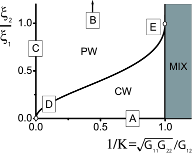
Figure 1: The wetting phase diagram at two-phase coexistence ($\mu_{{}_{2}}/\overline{\mu}_{{}_{2}}=1$) with phase $1$ imposed far from the wall, as a function of $\xi_{{}_{2}}/\xi_{{}_{1}}$ and $1/K=\sqrt{G_{{}_{11}}G_{{}_{22}}}/G_{{}_{12}}$. The wetting line connects the points $(0,0)$ and $(1,1)$ and separates the regions of partial wetting (PW, no absorbed film of phase 2) and complete wetting (CW, a macroscopic wetting layer of phase 2). When $1/K>1$, phases $1$ and $2$ mix and there, a (metastable) $1$-$2$ interface does not exist. The region indicated by letter A is treated in Sect. VI.1, region B with $\xi_{{}_{2}}/\xi_{{}_{1}}\rightarrow\infty$ in Sect. VI.2 and analogously for regions C, D and E.

The imposed boundary conditions are:

$$\Psi_{{}_{2}}(z=0)=\Psi_{{}_{1}}(0)=0,\,\Psi_{{}_{2}}(\infty)=0\text{ and }\Psi_{{}_{1}}(\infty)\equiv\sqrt{n_{{}_{1}}},$$ (2)

where $n_{{}_{1}}$ is the number density of the pure phase of condensate $1$ with fixed chemical potential $\mu_{{}_{1}}$ and self-interaction $G_{{}_{11}}$, i.e., $n_{{}_{1}}=\mu_{{}_{1}}/G_{{}_{11}}$. Note that the particle-wall interactions are solely mediated by the first two conditions in (2). The pure bulk phase pressures $P_{{}_{i}}$ and the chemical potential $\mu_{{}_{i}}$ are related by $P_{{}_{i}}=\mu_{{}_{i}}^{2}/(2G_{{}_{ii}})$ with $i=1,\,2$. Therefore, each value of $\mu_{{}_{1}}$ has an associated chemical potential for phase $2$, defined by $\overline{\mu}_{{}_{2}}\equiv\mu_{{}_{1}}\sqrt{G_{{}_{22}}/G_{{}_{11}}}$, such that at two-phase coexistence, i.e., when $P_{{}_{2}}=P_{{}_{1}}$, $\mu_{{}_{2}}$ equals $\overline{\mu}_{{}_{2}}$. We define $\overline{n}_{2}\equiv\overline{\mu}_{{}_{2}}/G_{{}_{22}}$.

IV The Wetting Phase Diagram

For the pure phases $1$ and $2$, the typical lengths of variation of wave functions $\Psi_{{}_{1}}$ and $\Psi_{{}_{2}}$ are the healing lengths $\xi_{{}_{1}}\equiv\hslash/\sqrt{2m_{{}_{1}}\mu_{{}_{1}}}$ and $\xi_{{}_{2}}\equiv\hslash/\sqrt{2m_{{}_{2}}\overline{\mu}_{{}_{2}}}$, respectively. We introduce two bulk parameters, namely $\xi_{{}_{2}}/\xi_{{}_{1}}$ and the inter-phase interaction parameter $K\equiv G_{{}_{12}}/\sqrt{G_{{}_{11}}G_{{}_{22}}}$. One can then rewrite $K$ and $\xi_{{}_{2}}/\xi_{{}_{1}}$ as a function of the masses $m_{{}_{i}}$ and scattering lengths $a_{{}_{ij}}$ as follows pita :

$$K=\frac{m_{{}_{1}}+m_{{}_{2}}}{2\sqrt{m_{{}_{1}}m_{{}_{2}}}}\frac{a_{{}_{12}}}{\sqrt{a_{{}_{11}}a_{{}_{22}}}}\text{ and }\xi_{{}_{2}}/\xi_{{}_{1}}=\sqrt[4]{\frac{m_{{}_{1}}a_{{}_{11}}}{m_{{}_{2}}a_{{}_{22}}}}.$$ (3)

For our purposes we assume $P_{{}_{1}}\geq P_{{}_{2}}$. In order to obtain pure phase 1 as the stable phase in bulk, $K$ must be larger than $\mu_{{}_{2}}/\overline{\mu}_{{}_{2}}=\sqrt{P_{{}_{2}}/P_{{}_{1}}}$, where the external parameter $1-\mu_{{}_{2}}/\overline{\mu}_{{}_{2}}$ quantifies the deviation from bulk two-phase coexistence. If, in addition, $P_{{}_{1}}=P_{{}_{2}}$, pure phase 1 and pure phase 2 coexist in bulk and the condition for phase separation then becomes $K>1$ ao .

The wetting phase diagram at bulk two-phase coexistence is depicted in Fig. 1. It shows that complete wetting is possible for practically every value of $K$ whenever $\xi_{{}_{2}}\ll\xi_{{}_{1}}$ and it can also occur for practically every value of $\xi_{{}_{2}}/\xi_{{}_{1}}\,(<1)$ in the regime of weak segregation, i.e., $(0<)\,K-1\ll 1$. The wetting line (WL), separating the partial wetting (PW) and the complete wetting (CW) regions indicates a first-order surface phase transition indekeu3 . On the WL, arbitrary film thicknesses can occur and are associated with an infinite degeneracy of the grand potential. This entails another peculiarity off of coexistence where this first-order WL is continued by a nucleation or prewetting line which is all the way of second order and, contrary to expectations, not tangential to the line of bulk coexistence at the wetting transition point indekeu3 .

The prewetting surface, which contains the WL at $\mu_{{}_{2}}/\overline{\mu}_{{}_{2}}=1$, satisfies vanschaeybroeck2 :

$$\sqrt{K-\mu_{{}_{2}}/\overline{\mu}_{{}_{2}}}=\frac{\sqrt{2}}{3}\left(\frac{\mu_{{}_{2}}/\overline{\mu}_{{}_{2}}}{\xi_{{}_{2}}/\xi_{{}_{1}}}-\xi_{{}_{2}}/\xi_{{}_{1}}\right).$$ (4)

In Sect. VI, we investigate the regions in the $(K,\xi_{{}_{2}}/\xi_{{}_{1}})$-space, indicated in Fig. 1 by the letters A through E.

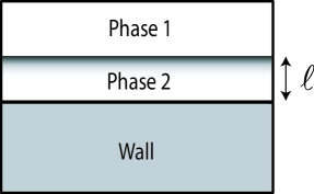
Figure 2: Configuration with pure phase 1 stable in bulk and an adsorbed film of pure species 2 at the wall. This configuration is homogeneous (i.e., translationally invariant in directions parallel to the wall). The interface potential $V(\ell)$ maps a configuration with a microscopic adsorbed film of species $2$ of thickness $\ell$, or a macroscopic wetting layer of pure phase 2 ($\ell\rightarrow\infty$), to its excess grand potential.

V The Interface Potential

V.1 Definition

The interface potential $V(\ell)$ relates a system with phase 1 imposed in bulk and an adsorbed film of phase 2 of thickness $\ell$ to its excess energy per unit area. In addition, in our convention the potential vanishes for a configuration with an infinitely thick film (macroscopic layer) at coexistence with the bulk. Therefore, one can write:

$$V(\ell)\equiv\gamma(\mu_{{}_{1}},\mu_{{}_{2}};\ell)-\gamma_{{}_{0}},$$ (5)

where we have added the argument $\ell$ in the functional $\gamma$ to highlight that $\gamma$ is evaluated for an adsorbed film of imposed thickness $\ell$, and where

$$\gamma_{{}_{0}}\equiv\left.\gamma(\mu_{{}_{1}},\overline{\mu}_{{}_{2}};\ell)\right|_{\ell=\infty}$$ (6)

We define the film thickness $\ell$ as:

$$\ell\equiv\Gamma/\overline{n}_{{}_{2}}\equiv\int_{{}_{0}}^{{}_{\infty}}\text{d}z\,\psi_{{}_{2}}^{2},$$ (7)

where $\Gamma$ is the adsorption of species $2$, being the excess particle number of species $2$ per unit area. This definition is a physically obvious way of relating the length $\ell$ to the (in principle) measurable quantity $\Gamma$. It is fortunate that the second power of $\psi$ is featured in the integral constraint (7). This implies that the constrained profiles are analytic everywhere (except at boundaries) and that the singularities that are known to occur when a crossing criterion is used boulter2 are absent in our approach.

Generally, states with arbitrary film thickness $\ell$ are unstable as they do not obey the principle of minimal energy for $\gamma$. The standard procedure to derive them nevertheless, using a variational principle, is to constrain state space to states with film thicknesses $\ell$, while assuming the potential $\gamma$ still describes the energy of the system. Thus, instead of $\gamma$, one must minimize

$$\widehat{\gamma}(\mu_{{}_{1}},\mu_{{}_{2}};\Pi)=\gamma(\mu_{{}_{1}},\mu_{{}_{2}};\ell)+\Pi\ell,$$ (8)

with respect $\psi_{{}_{1}}$ and $\psi_{{}_{2}}$. Here the disjoining pressure

$$\Pi\equiv-\partial V(\ell)/\partial\ell,$$ (9)

plays the role of a Lagrange multiplier. One therefore proceeds by first performing a variational procedure in order to get the optimal film thickness $\ell$ at fixed disjoining pressure, and subsequently deducing the interface potential. We denote the equations of state which minimize $\widehat{\gamma}$ with respect to the bosonic wave functions, by the modified GP equations. When the disjoining pressure vanishes, one recovers the equilibrium solutions for $\gamma$ which have the property to have no force exerted on the $1$-$2$ interface. In addition, one must also allow for the existence of boundary minima at which $\Pi\neq 0$, notably at $\ell=0$. Global minima in the form of boundary minima may also correspond to equilibrium solutions.

V.2 A Dynamical Point of View

By a “mechanical” analogy, used throughout this work, the modified GP equations can be reinterpreted as Newton’s equations of motion for two particles where the evolution in time must be replaced by a variation of the space coordinate $z$. The particles have one-dimensional “positions” $\psi_{{}_{i}}$ and “masses” $\hslash^{2}/(2m_{{}_{i}}\mu_{{}_{i}})$ and they move with kinetic energy $T$ in a potential $U$ (both per unit volume) footnote1 . Then,

$$U[\psi_{{}_{1}},\psi_{{}_{2}}] =2P_{{}_{1}}\left[\psi_{{}_{1}}^{2}+\eta\psi_{{}_{2}}^{2}-\frac{\psi_{{}_{1}}^{4}}{2}-\frac{\psi_{{}_{2}}^{4}}{2}-K\psi_{{}_{1}}^{2}\psi_{{}_{2}}^{2}\right],$$ (10a)

$$T[\dot{\psi}_{{}_{1}},\dot{\psi}_{{}_{2}}] =2P_{{}_{1}}\left[\xi_{{}_{1}}^{2}\dot{\psi^{2}_{{}_{1}}}+\xi_{{}_{2}}^{2}\dot{\psi^{2}_{{}_{2}}}\right].$$ (10b)

Here the dot denotes the derivative with respect to $z$, $\psi_{{}_{1}}\equiv\Psi_{{}_{1}}/\sqrt{n_{{}_{1}}}$ and $\psi_{{}_{2}}\equiv\Psi_{{}_{2}}/\sqrt{\overline{n}_{{}_{2}}}$. Here, the dimensionless parameter

$$\eta\equiv\frac{\mu_{{}_{2}}}{\overline{\mu}_{{}_{2}}}-\frac{\Pi}{2P_{{}_{1}}},$$ (11)

takes over the role of Lagrange multiplier from $\Pi$. Importantly, there is a one-to-one correspondence between the wave function profiles of thickness $\ell$ and the parameter $\eta$; therefore all wave profiles for configurations with fixed film thickness $\ell$ are the same, independently of $\mu_{{}_{2}}/\overline{\mu}_{{}_{2}}$. In other words, the nonequilibrium and equilibrium profiles of equal thickness $\ell$ are analytic and are the same at two-phase coexistence and off of coexistence, respectively, provided the latter exist as equilibrium states. A conservation of energy per unit volume links the kinetic to the potential energy at each point:

$$U[\psi_{{}_{1}},\psi_{{}_{2}}]+T[\dot{\psi}_{{}_{1}},\dot{\psi}_{{}_{2}}]=P_{{}_{1}},$$ (12)

obtained by a summation of the first integrals of the modified GP equations footnote2 .

V.3 Discussion on $V(\ell)$

We discuss the behavior of the interface potential before its explicit calculation. First, introduce the surface tensions of the pure phases 1 and 2 when adsorbed at the wall, $\gamma_{{}_{1W}}\equiv\gamma(\mu_{{}_{1}},\overline{\mu}_{{}_{2}};\ell=0)$ and $\gamma_{{}_{2W}}\equiv\gamma(\mu_{{}_{1}},\overline{\mu}_{{}_{2}};\ell=\infty)-\gamma_{{}_{12}}$, defined at two-phase coexistence using only $\mu_{{}_{1}}$ and $\overline{\mu}_{{}_{2}}$ and not $\mu_{{}_{2}}$, and with $\gamma_{{}_{12}}\equiv\gamma_{{}_{12}}(\mu_{{}_{1}},\overline{\mu}_{{}_{2}})$ the tension of the $1$-$2$ interface. Expressions for $\gamma_{{}_{12}}$ can be found in vanschaeybroeck and references therein; its qualitative dependence on $K$ is rather simple: $\gamma_{{}_{12}}$ is maximal in the limit of $K\rightarrow\infty$, decreases upon decrease of $K$ and vanishes at $K=1$.

It is instructive to reexpress the interface potential by use of (12) in the following form:

$$V(\ell)+\gamma_{{}_{0}} =2P_{{}_{1}}(1-\mu_{{}_{2}}/\overline{\mu}_{{}_{2}})\ell+2P_{{}_{1}}(\eta-1)\ell$$ (13)

$$+2\int_{{}_{0}}^{{}_{\infty}}\text{d}z\,T[\dot{\psi}_{{}_{1}}(z),\dot{\psi}_{{}_{2}}(z)].$$

Remarkably, in (13) we were able to isolate the part dependent on the deviation from bulk coexistence, which is the term proportional to $1-\mu_{{}_{2}}/\overline{\mu}_{{}_{2}}$. Indeed, as mentioned before, the wave functions for films with thickness $\ell$ are the same for different values of $1-\mu_{{}_{2}}/\overline{\mu}_{{}_{2}}$.

Starting with a configuration with only species $1$ at the wall, one gets $\left.V(\ell)\right|_{\ell=0}=\gamma_{{}_{1W}}-\gamma_{{}_{0}}$ and since $\left.V(\ell)\right|_{\ell=\infty}+\gamma_{{}_{0}}=\gamma_{{}_{2W}}+\gamma_{{}_{12}}$, we have that the difference $\left.V(\ell)\right|_{\ell=0}-\left.V(\ell)\right|_{\ell=\infty}$ corresponds to the spreading coefficient $\mathcal{S}$:

$$\mathcal{S}\equiv\gamma_{{}_{1W}}-(\gamma_{{}_{2W}}+\gamma_{{}_{12}}).$$ (14)

For a system at two-phase coexistence and in equilibrium, the spreading coefficient $\mathcal{S}$ is negative (for partial wetting) or zero (for complete wetting). A positive $\mathcal{S}$ corresponds to a nonequilibrium state which, in the course of time, may relax to a complete wetting equilibrium state (of lower excess energy) with $\mathcal{S}=0$. Note that since we define the interface potential to vanish in the limit $\ell=\infty$ at bulk two-phase coexistence, the partial wetting state ($\ell=0$ in our system) satisfies $\left.V(\ell)\right|_{\ell=0}=\mathcal{S}$.

To understand qualitatively how the parameters $\xi_{{}_{2}}/\xi_{{}_{1}}$ and $K$ influence the interface potential, we consider first a simple one-component (e.g., an adsorbed liquid-vapor or Ising-like) system. There, the form of the interface potential in the presence of interactions of short-range nature (ignoring van der Waals forces), is:

$$V(\ell)=h\ell+\sum_{m=1}^{\infty}A_{{}_{m}}e^{-m\ell/\xi_{{}_{c}}}.$$ (15)

Here $h$ is the bulk field and the expansion coefficients $A_{{}_{m}}$ are independent of $\mu_{{}_{2}}/\overline{\mu}_{{}_{2}}$. The length $\xi_{{}_{c}}$ corresponds to the bulk correlation length which is also the decay length of the tail in the interface profile. The dominant variation for large $\ell$ comes from the first term $A_{{}_{1}}e^{-\ell/\xi_{c}}$, at least when $A_{{}_{1}}\neq 0$.

Further on we will establish that an expression akin to (15), with exponentially decaying terms, gives the generic interface potential for the two-component BEC system. From (13), one sees that the bulk field corresponds to:

$$h=2P_{{}_{1}}(1-\mu_{{}_{2}}/\overline{\mu}_{{}_{2}}).$$ (16)

In analogy with the one-component system, one might expect the length $\xi_{{}_{c}}$ in the binary system to be either $\xi_{{}_{1}}$ or $\xi_{{}_{2}}$. However, we find that this is only true when the mutual penetration is small. Generally, $\xi_{{}_{c}}$ also depends on the interspecies repulsion parameter $K$.

Yet, (15) turns out inadequate to describe the interface potential in two regimes: 1) in Sect. VI.1, long-range correlations appear and $V(\ell)$ displays an extraordinary algebraic decay $V(\ell)\propto\ell^{-1}$ for large $\ell$, and 2) instead of one, two length scales determine the exponential decay of the interface potential found in Sect. VI.4. The competition and crossover behavior in the presence of two characteristic lengths was earlier encountered in hauge2 and in vanleeuwen ; KogaIW where it gave rise to non-universal critical wetting exponents that depend on the ratio of these two lengths.

One may wonder whether (16) is indeed what one expects for the bulk field. For a (nonequilibrium) system with a large film thickness $\ell$, the exponential contributions in (15) vanish such that the excess energy should be $\ell(P_{{}_{1}}-P_{{}_{2}})$ with $P_{{}_{i}}$ minus the derivative of $\Omega=\gamma-P_{{}_{1}}\mathcal{V}$ with respect to the volume $\mathcal{V}$, evaluated for pure bulk phase $i$. However, the bulk field in (16) is not exactly given by $P_{{}_{1}}-P_{{}_{2}}$, for the following reasons. The method to construct the state with large film thickness $\ell$, is to minimize the $\widehat{\gamma}$ which is constrained because of the applied disjoining pressure. This results in an equal pressure for pure phase $1$ and pure phase $2$, where the pressure is now the derivative of $\widehat{\Omega}=\widehat{\gamma}-P_{{}_{1}}\mathcal{V}$ with respect to the volume, again evaluated for the pure bulk phase. One easily calculates that the pure bulk phase density of phase $2$, obtained with $\widehat{\Omega}$, equals $\overline{\mu}_{{}_{2}}/G_{{}_{22}}$, rather than the density $\mu_{{}_{2}}/G_{{}_{22}}$ as obtained with $\Omega$ footnote3 . Eventually, $h=P_{{}_{1}}[-2(\mu_{{}_{2}}/\overline{\mu}_{{}_{2}})+1]-(-P_{{}_{1}})$ which is  (16). Note that a different choice of definition for $\ell$ would yield a different $h$.

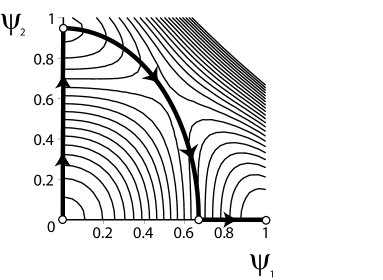
Figure 3: The trajectory in the coordinates $(\psi_{{}_{1}},\psi_{{}_{2}})$ for $\xi_{{}_{2}}/\xi_{{}_{1}}=0$, $K=2$ ($\eta=0.9$) with equipotential curves of $U$ in the background. The points $(1,0)$ and $(0,1)$ are maxima of $U$, whereas $(0,0)$ is a minimum and there exists a saddle point for the mixed phase in the middle. The upper right equipotential curves were left out due to their large density.

VI Results for the interface potential

VI.1 Strong Healing Length Asymmetry I

We focus in the following on the situation in which the adsorbed species $2$ has a much smaller healing length than species $1$ or $\xi_{{}_{2}}\ll\xi_{{}_{1}}$. Looking at region 1 in Fig. 1, complete wetting is expected at coexistence since $\mathcal{S}$ is identically zero. Indeed, first of all $\gamma_{{}_{2W}}$ is much smaller than the metastable extension of $\gamma_{{}_{1W}}$, denoted by $\gamma_{{}_{1W}}^{*}$ because $\gamma_{{}_{2W}}\propto\xi_{{}_{2}}$ and $\gamma_{{}_{1W}}^{*}\propto\xi_{{}_{1}}$, and secondly, $\gamma_{{}_{12}}\leq\gamma_{{}_{1W}}$. This ascertains the zero spreading coefficient.

According to the dynamical two-particle approach, $\xi_{{}_{2}}/\xi_{{}_{1}}=0$ means that particle 2 cannot gain momentum and will adapt its position to the potential which is modified by the moving particle $1$. We plot the evolution of the particle positions $(\psi_{{}_{1}},\psi_{{}_{2}})$ in Fig. 3 for a system with nonzero film thickness and $\xi_{{}_{2}}/\xi_{{}_{1}}=0$. Starting in the point $(0,0)$, particle $2$ jumps to position $\sqrt{\eta}$ on the short time scale $\xi_{{}_{2}}$. Then, particle $1$ starts to convert its potential to kinetic energy on a time scale $\Lambda_{{}_{1}}=\xi_{{}_{1}}/\sqrt{K-1}$, as seen from the modified GP equations since $\eta\rightarrow 1$ when $\ell\rightarrow\infty$:

$$\xi_{{}_{1}}^{2}\ddot{\psi}_{{}_{1}}=\psi_{{}_{1}}\left[\eta K-1+\psi_{{}_{1}}^{2}(1-K^{2})\right]\,\text{ and }\,\psi_{{}_{2}}^{2}=\eta-K\psi_{{}_{1}}^{2}.$$ (17)

Then, particle 2 is stopped abruptly at the position $\psi_{{}_{2}}=0$ when $\psi_{{}_{1}}=\sqrt{\eta/K}$. This abruptness is allowed by a lack of momentum of the massless particle $2$. Subsequently, particle $1$ continues climbing the potential hill, reaching the top $\psi_{{}_{1}}=1$ only after an infinite amount of time.

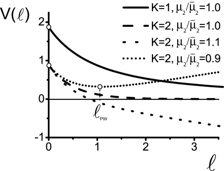
Figure 4: Interface potential $V(\ell)$ in units of $P_{{}_{1}}\xi_{{}_{1}}$ as a function of the film thickness $\ell$ in units of $\xi_{{}_{1}}$ when $\xi_{{}_{2}}/\xi_{{}_{1}}=0$. The curve for $K=2$ and $\mu_{{}_{2}}/\overline{\mu}_{{}_{2}}=1$ follows an exponential decay whereas the slow decay for $K=1$ is described by a power law. The thickness $\ell_{{}_{\rm PW}}$ indicates the thickness of the prewetting film for $K=2$ and $\mu_{{}_{2}}/\overline{\mu}_{{}_{2}}=0.9$ when phase 1 is stable in bulk and phase 2 is metastable. No such local minimum, or prewetting film of phase 2, exists when $\mu_{{}_{2}}/\overline{\mu}_{{}_{2}}>1$ because phase 1 is not stable in bulk.

The particles then follow the equations of motion:

$$\xi_{{}_{1}}^{2}\ddot{\psi}_{{}_{1}}=\psi_{{}_{1}}\left[-1+\psi_{{}_{1}}^{2}\right]\quad\text{ and }\quad\psi_{{}_{2}}=0.$$ (18)

In the Appendix we give the exact interface potential $V(\ell)$ together with the applied analytic methods for this case $\xi_{{}_{2}}/\xi_{{}_{1}}=0$. We show $V(\ell)$ in Fig. 4 for $K=1$ and $K=2$, the latter for different values of $\mu_{{}_{2}}/\overline{\mu}_{{}_{2}}$. For large $\ell$ and $K\neq 1$, we derive the leading terms:

$$V(\ell)=h\ell+\overline{A}_{{}_{1}}P_{{}_{1}}\xi_{{}_{1}}e^{-2\ell\sqrt{K+1}/\xi_{{}_{1}}}+\ldots$$ (19)

with $\overline{A}_{{}_{1}}$ given in (53) and $\overline{A}_{{}_{1}}\rightarrow 0$ when $K\rightarrow 1$ and $K\rightarrow\infty$. The fact that the decay length $\xi_{{}_{c}}=\xi_{{}_{1}}/(2\sqrt{K+1})$ contains the parameter $K$ expresses that the film thickness is chiefly modified by a changing overlap between both species. The interface potential is a monotonically decaying function for which both the decay length $\xi_{{}_{c}}$ and $V(0)$ decrease with increasing $K$ (see Fig. 4). Indeed, upon increase of $K$, $V(0)$ goes down due to the increase of $\gamma_{{}_{12}}$.

For low pressure of the adsorbed species $2$, when $\mu_{{}_{2}}/\overline{\mu}_{{}_{2}}<1$, the energy necessary to adsorb a large film increases linearly with its thickness. Nevertheless, for every $\mu_{{}_{2}}/\overline{\mu}_{{}_{2}}$, there exists an energy minimum for thin prewetting film thickness $\ell_{{}_{\rm PW}}$ (short dotted line in Fig. 4). By a simple calculation using (19), it is shown that the prewetting film thickness $\ell_{{}_{\rm PW}}$ diverges logarithmically slowly for $\mu_{{}_{2}}/\overline{\mu}_{{}_{2}}\uparrow 1$. Its asymptotic behavior is given by

$$\ell_{{}_{\rm PW}}\sim-(\xi_{{}_{1}}/(2\sqrt{K+1}))\ln(1-\mu_{{}_{2}}/\overline{\mu}_{{}_{2}}).$$ (20)

As weak segregation is approached, i.e., $K\rightarrow 1$, the length $\xi_{{}_{c}}\rightarrow\xi_{{}_{1}}/(2\sqrt{2})$ remains finite, while the coefficient $\overline{A}_{{}_{1}}$ vanishes footnote4 . At the bulk demixing point, i.e., when $K=1$, one can obtain from (2) a power-law form for the interface potential:

$$V(\ell)=h\ell+\frac{\pi^{2}P_{{}_{1}}\xi_{{}_{1}}}{8(\ell/\xi_{{}_{1}})}-\frac{\pi^{3}P_{{}_{1}}\xi_{{}_{1}}}{256(\ell/\xi_{{}_{1}})^{3}}+\ldots$$ (21)

This potential is also depicted in Fig. 4 for $\mu_{{}_{2}}/\overline{\mu}_{{}_{2}}=1$. From (21), one can notice the long-ranged nature (algebraic decay) of $V(\ell)-h\ell$ since it is proportional to $1/\ell$. This interface potential predicts that the equilibrium configuration in the limit $K\downarrow 1$ consists of a 1-2 interface that is delocalised from the surface. This interface, at $K=1$, has interfacial tension zero but nevertheless possesses a non-vanishing wave function profile that connects the two pure phases in bulk and that is of infinite width as determined by the diverging interspecies penetration depths $\xi_{i}/\sqrt{K-1}$, $i=1,2$. This divergence is reminiscent of a divergent correlation length and in that sense the limit $K\downarrow 1$ is akin to an approach to criticality, but with still two distinct coexisting pure phases 1 and 2 in bulk.

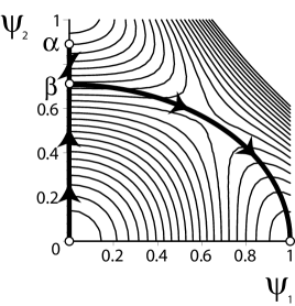
Figure 5: The trajectory for $(\psi_{{}_{1}},\psi_{{}_{2}})$ with $\xi_{{}_{1}}/\xi_{{}_{2}}=0$, $K=2$ and $\eta=1.02$. Starting at position $(0,0)$, the path goes to $\alpha=(\sqrt{\eta},0)$ where it turns back to the point $\beta=(\sqrt{1/K},0)$. Further, both $\psi_{{}_{1}}$ and $\psi_{{}_{2}}$ are nonzero up to the point $(0,1)$.

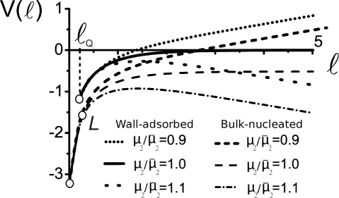
Figure 6: Interface potential $V(\ell)$ in units of $P_{{}_{1}}\xi_{{}_{2}}$ as a function of the film thickness $\ell$ in units of $\xi_{{}_{2}}$ for the wall-adsorbed and the bulk-nucleated states when $\xi_{{}_{1}}/\xi_{{}_{2}}=0$ and $K=5$ and for different $\mu_{{}_{2}}/\overline{\mu}_{{}_{2}}$. The point $L$ indicates a stratification point where pure phase $1$ is separated into two regions due to a planar film of pure phase $2$ parallel to but infinitely far from the wall. Note that the thickness $\ell$ which corresponds to the point $L$ does not equal $\ell_{{}_{Q}}$. The latter is the initial point of the potential of the wall-adsorbed state for all values of $\mu_{{}_{2}}/\overline{\mu}_{{}_{2}}$. However, the values of the potential for the three different values of $\mu_{{}_{2}}/\overline{\mu}_{{}_{2}}$ at $\ell_{{}_{Q}}$, differ slightly; this is not visible. It is obvious that we are in the partial wetting regime and that for all values for $\ell$, the bulk-nucleated state has the lower excess energy.

The previous discussion was for $\xi_{{}_{2}}/\xi_{{}_{1}}=0$. If one sets $\xi_{{}_{2}}/\xi_{{}_{1}}$ to a small but non-zero value, the most significant change to $V(\ell)$ is a decrease of the spreading coefficient $V(0)$, caused by a modification of the wave function $\psi_{{}_{2}}$ at both locations where it vanishes vanschaeybroeck . One location is near the surface, where a negative correction linear in $\xi_{{}_{2}}/\xi_{{}_{1}}$ is incurred. The second location is in the 1-2 interface where a positive correction quadratic in $\xi_{{}_{2}}/\xi_{{}_{1}}$ results vanschaeybroeck .

VI.2 Strong Healing Length Asymmetry II

We concentrate now on the inverse case $\xi_{{}_{1}}\ll\xi_{{}_{2}}$. As one expects, partial wetting is met, evidenced by a negative spreading coefficient since $\gamma_{{}_{1W}}\ll\gamma_{{}_{2W}}$. Species $2$ is so strongly disfavored near the wall, that it rather nucleates in the bulk. Indeed, we find that “wall-adsorbed states” attain a higher energy than “bulk-nucleated states” with the same thickness $\ell$ and where the latter are planar bulk states or essentially one-dimensional stationary soliton states. Henceforth, we focus on the limiting case $\xi_{{}_{1}}/\xi_{{}_{2}}=0$. A general two-particle trajectory for wall-adsorbed states is given in Fig. 5. Particle $2$ starts at position $(0,\,0)$ and reaches its maximal position $\alpha$ over a time scale $\xi_{{}_{2}}$, where it reverts its motion, up to the point $\beta=(0,\sqrt{1/K})$. This evolution is described by:

$$\xi_{{}_{2}}^{2}\ddot{\psi}_{{}_{2}}=\psi_{{}_{2}}\left[-\eta+\psi_{{}_{2}}^{2}\right]\quad\text{ and }\quad\psi_{{}_{1}}=0.$$ (22)

When $\psi_{{}_{2}}$ reaches the point $\beta$ for the second time, $\psi_{{}_{1}}$ becomes nonzero and in analogy with the last section, the conversion of kinetic to potential energy is achieved on a time scale $\Lambda_{{}_{2}}=\xi_{{}_{2}}/\sqrt{K-1}$ as may be seen from:

$$\xi_{{}_{2}}^{2}\ddot{\psi}_{{}_{2}}=\psi_{{}_{2}}\left[\eta K-1+\psi_{{}_{2}}^{2}(1-K^{2})\right]\,\text{ and }\,\psi_{{}_{1}}^{2}=\eta-K\psi_{{}_{2}}^{2}.$$ (23)

A remarkable feature is encountered when considering small adsorption $\ell$; $V(\ell)$ is found not to exist when $\ell<\ell_{{}_{Q}}$. A similar phenomenon was observed in the context of the interface potential for superconducting surface sheaths in Ginzburg-Landau theory blossey . This “quantum” effect arises because, spatially seen, the wave function $\psi_{{}_{2}}(z)$ is constrained to vanish at $z=0$ and to have the value $\sqrt{1/K}$ at a certain point $z=z_{{}_{0}}$; wave solutions therefore do not exist for too small values of $z_{{}_{0}}$. Expression (54a) gives the interface potential which is shown in Fig. 6 for $K=5$ and for different values of $\mu_{{}_{2}}/\overline{\mu}_{{}_{2}}$. The quantum effect is apparent in Fig. 6 at the thickness $\ell_{{}_{Q}}$, being the minimal thickness for which the interface potential is defined.

Although we were unable to expand the potential in terms of large $\ell$, we can point out its principal feature. For large film thicknesses, the penetration depth of species $2$ into species $1$ (the bent path in Fig. 5) saturates, such that the film is grown from phase $2$, with $\psi_{{}_{1}}=0$ (the vertical path in Fig. 5). Therefore, the decay length of the interface potential is $\xi_{{}_{c}}=\xi_{{}_{2}}/2$. Contrary to findings of Sect. VI.1, $\xi_{{}_{c}}$ does not change with $K$, and $|V(0)|$ increases for larger values of $K$. Also, one can prove that for weak segregation, the thickness $\ell_{{}_{Q}}$ (see Fig. 6) diverges logarithmically with $K-1$ such that the interface potential is not well-defined when $K=1$.

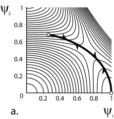
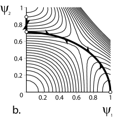
Figure 7: The paths followed by the coordinates $(\psi_{{}_{1}},\psi_{{}_{2}})$ in the case of “bulk excitations” when $\xi_{{}_{1}}/\xi_{{}_{2}}=0$, $K=2$ and $\eta=1.3$ (a) and $\eta=1.02$ (b). Both paths start in the point $(0,1)$ and finally return to this point.

The trajectories of the coordinates $(\psi_{{}_{1}},\psi_{{}_{2}})$ for “bulk-nucleated states” with a finite “adsorption” are shown in Fig. 7a and 7b. It is interesting to note the existence of a stratification point $L$ for these states (see Fig. 6), where the intrusion of species $2$ is sufficient to sever space in two parts of pure phase $1$. In Fig. 6, we compare $V(\ell)$ with the excess energy $\gamma$ of the bulk states which have the same “adsorption”, by subtraction of $\gamma_{{}_{0}}$. We found numerically that at coexistence the bulk states have a lower energy for all thicknesses $\ell$ and this is valid for all values of $K$ footnote5 .

When $\ell=\infty$, the condition for the excess energy of the “bulk-nucleated states” $\gamma_{{}_{1W}}+2\gamma_{{}_{12}}$ to be lower than the excess energy of the “wall-adsorbed states” $\gamma_{{}_{12}}+\gamma_{{}_{2W}}$ yields the complete drying condition $\gamma_{{}_{1W}}+\gamma_{{}_{12}}=\gamma_{{}_{2W}}$. In other words, if pure phase $2$ were to be the bulk phase, pure phase $1$ would wet the wall. This was already encountered in  indekeu . Lastly, we note that it is not clear whether or not the quantum effect disappears once we take $\xi_{{}_{1}}/\xi_{{}_{2}}\neq 0$.

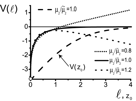
Figure 8: Interface potential $V(\ell)$ in units of $P_{{}_{1}}\xi_{{}_{2}}$ as a function of the film thickness $\ell$ in units of $\xi_{{}_{2}}$ when $1/K=0$ and for different values of $\mu_{{}_{2}}/\overline{\mu}_{{}_{2}}$ as a function of both $\ell$ and $z_{{}_{0}}$ where the value of $z_{{}_{0}}$ is determined by the locus of the $1$-$2$ interface. The state of lowest energy corresponds to zero film thickness. Note the steep increase of the potential as a function of small $\ell$ whereas $V$ varies linearly as a function of $z_{{}_{0}}$ for small values of $z_{{}_{0}}$. This behavior for small $\ell$ and small $z_{0}$ is due to the shift of the wave function profile of species $1$ with just a few particles of species $2$ being adsorbed at the surface.

VI.3 Strong Segregation

The condition $1/K=0$ induces species $1$ and $2$ to have no overlap such that the densities of both species vanish at a certain distance $z_{{}_{0}}$ from the wall (at least whenever $\ell\neq 0$). Since, in that case, $\gamma_{{}_{12}}=\gamma_{{}_{2W}}+\gamma_{{}_{1W}}$, partial wetting immediately follows from $\mathcal{S}<0$. Only density variations of adsorbed phase $2$ modify the interface potential. In fact, “inflating” the wetting layer merely shifts the density profile of species $1$, being $\psi_{{}_{1}}=\tanh[(z-z_{{}_{0}})/(\sqrt{2}\,\xi_{{}_{1}})]$ through an increase of $z_{{}_{0}}$. Species $2$ replaces species $1$ in the shifted region, thereby modifying its own density profile. The exact interface potential is provided in (2) and can be seen in Fig. 8 as a function of both $\ell$ and $z_{{}_{0}}$. For large $\ell$, we derived that footnote6 :

$$V(\ell)=h\ell-32\sqrt{2}\,P_{{}_{1}}\xi_{{}_{2}}\,e^{-(4+\sqrt{2}\,\ell/\xi_{{}_{2}})}+\ldots$$ (24)

and $V(z_{{}_{0}})$ is found using the relation $z_{{}_{0}}=\ell-2\sqrt{2}\,\xi_{{}_{2}}$, also valid for large $\ell$. Note that (24) can also be obtained by constraining the value of $z_{{}_{0}}$ instead of $\ell$. In Fig. 8, one observes an important difference between $V(\ell)$ and $V(z_{{}_{0}})$ for small values of $\ell$ and $z_{{}_{0}}$. This difference can be attributed to a feature which is reminiscent of the quantum effect as encountered in Sect. VI.2. Indeed, wave function $\psi_{{}_{2}}(z)$ is constrained to vanish at $z=0$ and at $z=z_{{}_{0}}$. By application of a sufficiently large disjoining pressure, solutions exist for all values of $\mu_{{}_{2}}/\overline{\mu}_{{}_{2}}$. For a fixed small value of the potential, the adsorption $\ell$ remains very small whereas the corresponding value for $z_{{}_{0}}$ increases linearly. Therefore, for low values of $z_{{}_{0}}$, the potential $V(z_{{}_{0}})$ roughly quantifies the energy needed to push species $1$ to a distance $z_{{}_{0}}$ from the wall and this is linear in $z_{{}_{0}}$.

When $1/K$ is small but nonzero, an overlap region of the condensates induces corrections to $\gamma_{{}_{12}}$ and therefore $V(0)$ of order $1/\sqrt[4]{K}$. It is then possible to sketch the evolution of $\psi_{{}_{1}}$ and $\psi_{{}_{2}}$ as was done for $K=1000$ in Fig. 9a. One sees the extreme deformation of the potential by dense contour lines when both densities are nonzero.

In fact, the above analysis is only valid when $1/\sqrt{K}\ll\xi_{{}_{2}}/\xi_{{}_{1}}$. In the following section we study the intermediate region in which $\xi_{{}_{2}}/\xi_{{}_{1}}\approx 1/\sqrt{K}$ and small compared to unity.

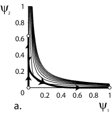
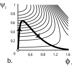
Figure 9: a) The path for $(\psi_{{}_{1}},\psi_{{}_{2}})$ when $K=1000$ and $\eta=1.1$. In the upper right corner, we left out the equipotential curves due to their high density. b) A part of the path followed by $(\phi_{{}_{1}},\psi_{{}_{2}})$ for $\kappa=0.5$ and $\eta=1.4$. In the continuation of the depicted path, $\psi_{{}_{2}}\rightarrow 0$ while $\phi_{{}_{1}}$ increases.

VI.4 Both Strong Segregation and Strong Healing Length Asymmetry

As indicated in Fig. 1, a transition from PW to CW occurs in regions E and D. These two regimes have in common the existence of two important length scales; one length scale near the wall and one length scale far from it, and therefore turn out more difficult to solve, especially numerically. However, upon approach of the points $(\xi_{{}_{2}}/\xi_{{}_{1}},1/K)=(0,0)$ and $(1,1)$, one length will be much larger than the other such that the analysis can be performed on two length scales separately.

Next, we treat the case when both $\xi_{{}_{2}}\ll\xi_{{}_{1}}$ and $1/K\ll 1$ while

$$\kappa\equiv\left[[\xi_{{}_{2}}/\xi_{{}_{1}}]\sqrt{K}\right]^{-1},$$ (25)

is of order unity vanschaeybroeck . In this limit and at coexistence, PW is encountered when $\kappa<3/\sqrt{2}$ while CW is found when $\kappa>3/\sqrt{2}$; this may be deduced from (4) and seen in Fig. 1. The associated important length scales are $\xi_{{}_{2}}$, near the wall and a much larger $\xi_{{}_{1}}$, far from the wall. Whereas the largest energy contribution is governed by density variations on the latter scale, the phenomena on the former scale decide whether there is PW or CW.

Let us first focus on the density variations close to the wall. We introduce the rescaling $\overline{z}\equiv z/\xi_{{}_{2}}$ and a new wave function $\phi_{{}_{1}}$ as in vanschaeybroeck following the calculational approach taken in boulter ; boulter3 :

$$\psi_{{}_{1}}= \,[\xi_{{}_{2}}/\xi_{{}_{1}}]\left[\phi_{{}_{1}}-\frac{\Theta(\overline{z}-\delta)(\overline{z}-\delta)}{\sqrt{2}}\right]$$ (26)

$$\quad+\Theta(z-\delta\xi_{{}_{2}})\tanh\left(\frac{z-\delta\xi_{{}_{2}}}{\sqrt{2}\xi_{{}_{1}}}\right),$$

where $\phi_{{}_{1}}$ must have the asymptotic behavior $\phi_{{}_{1}}(\overline{z}\rightarrow\infty)\sim(\overline{z}-\delta)/\sqrt{2}$ and $\phi_{{}_{1}}(\overline{z}\rightarrow-\infty)=0$. The scaling, $\psi_{{}_{1}}\propto\xi_{{}_{2}}/\xi_{{}_{1}}$ stems from the fact that $\psi_{{}_{1}}$ makes variations of order unity over a length $\xi_{{}_{1}}$ and hence variations of order $\xi_{{}_{2}}/\xi_{{}_{1}}$ over the length scale $\xi_{{}_{2}}$. Close to the wall, one can expand $U$ and $T$ to zeroth order in $\xi_{{}_{2}}/\xi_{{}_{1}}$ and in $1/K$:

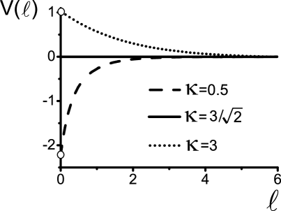
Figure 10: The numerically obtained interface potential $V(\ell)$ in units of $P_{{}_{1}}\xi_{{}_{2}}$ as a function of the film thickness $\ell$ in units of $\xi_{{}_{2}}$ for the case $\xi_{{}_{2}}\ll\xi_{{}_{1}}$ and $1/K\ll 1$ while $\kappa=\left[[\xi_{{}_{2}}/\xi_{{}_{1}}]\sqrt{K}\right]^{-1}$ is finite. We see that one encounters CW for $\kappa>3/\sqrt{2}$ and PW for $\kappa<3/\sqrt{2}$. These regimes are separated by the extraordinary flat potential.

$$U[\phi_{{}_{1}},\psi_{{}_{2}}] =2P_{{}_{1}}\left[\eta\psi_{{}_{2}}^{2}-\frac{\psi_{{}_{2}}^{4}}{2}-\frac{\phi_{{}_{1}}^{2}\psi_{{}_{2}}^{2}}{\kappa^{2}}\right],$$ (27a)

$$T[\dot{\phi_{{}_{1}}},\dot{\psi_{{}_{2}}}] =2P_{{}_{1}}\left[\dot{\phi_{{}_{1}}^{2}}+\dot{\psi^{2}_{{}_{2}}}\right],$$ (27b)

where the dot now indicates the derivative with respect to $\overline{z}$. The extension to the region far from the wall (where $z\gg\xi_{{}_{2}}$) is made by observing that there $\psi_{{}_{2}}=0$ while $\phi_{{}_{1}}$ goes over into a $\tanh$ profile. By straightforward calculation, one can write the interface potential as:

$$V(\ell)= \,4P_{{}_{1}}\xi_{{}_{2}}\int_{{}_{0}}^{{}_{\infty}}\text{d}\overline{z}\,\left[\left(\dot{\phi}_{{}_{1}}-\frac{1}{\sqrt{2}}\right)^{2}+\dot{\psi}_{{}_{2}}^{2}\right]$$

$$-\Pi\ell-2\delta P_{{}_{1}}\xi_{{}_{2}}-\gamma_{{}_{12}},$$ (28)

In Fig. 10 we depict the interface potential for different values of $\kappa$. The results are obtained by a numerical integration of the profiles, followed by the evaluation of the potential with the functional (VI.4). Clearly we see that the transition from PW to CW is mediated by a completely flat potential for $\kappa=3/\sqrt{2}$. The constancy of the interface potential is a property of crucial importance in the context of the wetting phase transition in this model. It corroborates the earlier observation of the infinite degeneracy of the grand potential at first-order wetting indekeu3 . This property is in stark contrast with the normally expected and ubiquitous double-minima structure of $V(\ell)$ at first-order wetting.

We proceed by arguing that the interface potential in the limit under consideration should have the form:

$$V(\ell)=h\ell+Ce^{-\sqrt{2}\,\ell/\xi_{{}_{2}}}+De^{-2\sqrt{K}\,\ell/\xi_{{}_{1}}}+\ldots$$ (29)

where the amplitudes $C$ and $D$ are independent of $\ell$ and positive such that no critical wetting transition is possible hauge . First of all, for small values of $\kappa$ and thus $\xi_{{}_{2}}/\xi_{{}_{1}}\ll\sqrt{K}$, $V(\ell)-h\ell$, for large $\ell$, should be the one obtained in Sect. VI.2 and thus be proportional to $e^{-\sqrt{2}\,\ell/\xi_{{}_{2}}}$, which means that $\xi_{{}_{c}}=\xi_{{}_{2}}/\sqrt{2}$. For large values of $\kappa$, i.e., $\sqrt{K}\ll\xi_{{}_{2}}/\xi_{{}_{1}}$, we must obtain the same result as obtained in Sect. VI.1 which is that $\xi_{{}_{c}}=\xi_{{}_{1}}/(2\sqrt{K})=\kappa\,\xi_{{}_{2}}/2$.

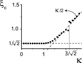
Figure 11: Plot for the numerically obtained length $\xi_{{}_{c}}$ in units of $\xi_{{}_{2}}$ in the case of $\xi_{{}_{2}}\ll\xi_{{}_{1}}$ and $1/K\ll 1$. This length characterizes the exponential decay for large $\ell$. The transition from $\xi_{{}_{c}}=1/\sqrt{2}$ for low values of $\kappa$ to $\xi_{{}_{c}}=\kappa/2$ is obvious. For values of $\kappa$ lower than $3/\sqrt{2}$, we are in the PW regime whereas for higher values, CW occurs.

These considerations are supported by fitting the numerically obtained values for $\xi_{{}_{c}}$ as a function of $\kappa$, as shown in Fig. 11. One observes that, indeed, $\xi_{{}_{c}}$ takes the value $\xi_{{}_{2}}/\sqrt{2}$ for low $\kappa$ and the value $\kappa\,\xi_{{}_{2}}/2$ for larger values of $\kappa$ footnote7 . Note that for different types of surfaces (involving softer walls) also critical wetting transitions have been established in GP theory vanschaeybroeck2 .

VI.5 Weak Segregation

We now direct our attention to the case when both $0<K-1\ll 1$ and $0<\xi_{{}_{1}}/\xi_{{}_{2}}-1\ll 1$. In this regime we will show that the transition from PW to CW at coexistence, mediated by a flat interface potential, takes place when $\sqrt{K-1}=2\sqrt{2}(\xi_{{}_{1}}/\xi_{{}_{2}}-1)/3$, as is readily deduced from (4). In the following, we take the Lagrange multiplier to be $\Pi=2P_{{}_{1}}\mu_{{}_{2}}/\overline{\mu}_{{}_{2}}$; in order to fix the film thickness, we use instead a parameter which is featured in our expansion. The expansion parameters are $\sqrt{K-1}\ll 1$ and $\xi_{{}_{1}}/\xi_{{}_{2}}-1\ll 1$ and we assume both to be of the same order. We extend a method, used earlier by Malomed et al. malomed and Mazets mazets for the calculation of the interfacial tension. In the limit $K\rightarrow 1$, the potential $U$ of (10a) is rotationally invariant; it is then natural to rewrite $\psi_{{}_{1}}$ and $\psi_{{}_{2}}$ as follows:

$$\psi_{{}_{1}}\equiv\,g(z)\sin[\chi(z)],$$ (30a)

$$\psi_{{}_{2}}\equiv\,g(z)\cos[\chi(z)],$$ (30b)

where the boundary conditions (2) imply $\left.g(z)\right|_{z=0}=0$, $\left.\chi(z)\right|_{z=0}<\pi/2$, $\left.\chi(z)\right|_{z=\infty}=\pi/2$ and $\left.g(z)\right|_{z=\infty}=1$. The existence of two largely different length scales $\xi_{{}_{2}}$ and $\xi_{{}_{2}}/\sqrt{K-1}$ gives rise to an expansion in its most general form:

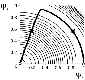
Figure 12: The path for the normalized densities in the case of weak segregation with $K=\xi_{{}_{1}}/\xi_{{}_{2}}=1.001$ and $\chi(0)=0.3$. Notice the (near-)rotational symmetry of the underlying potential $U$.

$$\chi(z)= \chi_{{}_{0}}(z)+\chi_{{}_{1}}(z\sqrt{K-1})$$ (31a)

$$+\sqrt{K-1}\,\chi_{{}_{2}}(z)\ldots,$$

$$g(z)= g_{{}_{0}}(z)+g_{{}_{1}}(z\sqrt{K-1})+\sqrt{K-1}\,g_{{}_{2}}(z)$$ (31b)

$$\quad+\sqrt{K-1}\,g_{{}_{3}}(z\sqrt{K-1})+\ldots$$

Here, $\chi_{{}_{1}}$, $g_{{}_{1}}$ and $g_{{}_{3}}$ vary as a function of the “slow coordinate” $z\sqrt{K-1}$ whereas $g_{{}_{0}}$, $g_{{}_{2}}$, $\chi_{{}_{2}}$ and $\chi_{{}_{0}}$ vary on the short length scale $\xi_{{}_{2}}$ near the wall. Expanding the modified GP equations in the small parameters $\sqrt{K-1}$ and $\xi_{{}_{1}}/\xi_{{}_{2}}-1$ and equating the same orders of magnitude, leads to:

$$\chi_{{}_{0}}=g_{{}_{1}}= g_{{}_{3}}=0,$$ (32a)

$$\xi_{{}_{2}}^{2}\ddot{g}_{{}_{0}}=- g_{{}_{0}}+g_{{}_{0}}^{3},$$ (32b)

$$\xi_{{}_{2}}^{2}\ddot{g}_{{}_{2}}=g_{{}_{2}}[-1+3g_{{}_{0}}^{2}] -2\left(\frac{\xi_{{}_{1}}/\xi_{{}_{2}}-1}{\sqrt{K-1}}\right)\xi_{{}_{2}}^{2}\ddot{g}_{{}_{0}}\sin[\chi_{{}_{1}}(0)],$$ (32c)

$$2\dot{g}_{{}_{0}}\dot{\chi}+\ddot{\chi}_{{}_{2}}=- (\xi_{{}_{1}}/\xi_{{}_{2}}-1)\ddot{g}_{{}_{0}}\sin^{2}[2\chi_{{}_{1}}(0)],$$ (32d)

$$\xi_{{}_{2}}\dot{\chi}_{{}_{1}}=- \sqrt{K-1}\,\frac{\sin 2\chi_{{}_{1}}}{2}.$$ (32e)

The last expression is obtained by setting $g=1$ and taking the first-order terms of the subtraction of the GP equations. In the third and fourth expression, we expand $\chi_{{}_{1}}(z)=\chi_{{}_{1}}(0)+\sqrt{K-1}\,\chi_{{}_{2}}(z)+\mathcal{O}(K-1)$ about its value at the wall; this is justified since $g_{{}_{2}}$ is nonzero only near the wall. The solutions are (with $K\neq 1$):

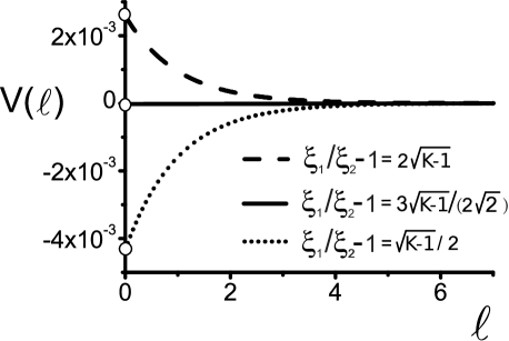
Figure 13: Interface potential $V(\ell)$ in units of $P_{{}_{1}}\xi_{{}_{2}}$ as a function of the film thickness $\ell$ in units of $\xi_{{}_{2}}/(2\sqrt{K-1})$ for weak segregation and small $\xi_{{}_{1}}/\xi_{{}_{2}}-1$. Here, $\sqrt{K-1}=0.01$ while $\xi_{{}_{1}}/\xi_{{}_{2}}-1$ varies. At the point where $\xi_{{}_{1}}/\xi_{{}_{2}}-1=3\sqrt{K-1}/(2\sqrt{2})$, we go over from PW to CW through a flat potential.

$$g_{{}_{0}}(z) =\tanh[z/(\sqrt{2}\,\xi_{{}_{2}})],$$ (33a)

$$g_{{}_{2}}(z) =\left(\frac{\xi_{{}_{1}}/\xi_{{}_{2}}-1}{\sqrt{K-1}}\right)\sin^{2}[\chi_{{}_{1}}(0)](g_{{}_{0}}^{2}-1)\text{arctanh}\,g_{{}_{0}},$$ (33b)

$$\chi_{{}_{1}}(z) =\text{arctanh}\left(e^{-\sqrt{K-1}\,z/\xi_{{}_{2}}}\tanh[\chi_{{}_{1}}(0)]\right).$$ (33c)

The solution for $\chi_{{}_{2}}$ is irrelevant for our further analysis. The value of $\chi_{{}_{1}}(0)$ is undetermined and we use this parameter to tune the film thickness. The interface potential can now be separated into a part close and a part far from the wall. It is interesting that, independently of the film thickness, both density profiles vary on the small length scale $\xi_{{}_{2}}$ close to the wall, whereas a length scale $\xi_{{}_{2}}/\sqrt{K-1}$ is found for the behavior far from the wall. Note that this set of equations is consistent with an expansion of the conservation of energy.

By use of (12) and (13), we then find to first order in $\sqrt{K-1}$:

$$\frac{V(\ell)+\gamma_{{}_{0}}-h\ell}{2P_{{}_{1}}}= \int_{{}_{0}}^{{}_{\infty}}\text{d}z\left[(1-g_{{}_{0}}^{2})^{2}+(K-1)\frac{\sin 2\chi_{{}_{1}}}{4}\right.$$

$$\left.+4\sqrt{K-1}\,g_{{}_{0}}g_{{}_{2}}(g_{{}_{0}}^{2}-1)\right]+\ldots,$$ (34)

while the expression for the film thickness is

$$\ell=\int_{{}_{0}}^{{}_{\infty}}\text{d}z\left[(g_{{}_{0}}^{2}-1)\cos^{2}[\chi_{{}_{1}}(0)]+\cos^{2}\chi_{{}_{1}}\right]+\mathcal{O}(\sqrt{K-1}).$$ (35)

Both $\ell$ and $V(\ell)$ depend on $\chi_{{}_{1}}(0)$ in such a way that this parameter can be eliminated. One can derive the exact interface potential to first order in $\sqrt{K-1}$ and to first order in $\xi_{{}_{1}}/\xi_{{}_{2}}-1$, which we give in (58); for large $\ell$ it reduces to:

$$V(\ell)= h\ell+2P_{{}_{1}}\xi_{{}_{2}}\left[\frac{2\sqrt{2}}{3}(\xi_{{}_{1}}/\xi_{{}_{2}}-1)-\sqrt{K-1}\right]$$

$$\times\exp\left(-\frac{2\ell\sqrt{K-1}}{\xi_{{}_{2}}}\right)+\ldots$$ (36)

Obviously, when $h=0$ and

$$\sqrt{K-1}=2\sqrt{2}(\xi_{{}_{1}}/\xi_{{}_{2}}-1)/3,$$ (37)

this interface potential, as well as the exact one in (58), vanishes for all $\ell$. Note that here, as opposed to the case in Sect. VI.4, only one length scale, namely $\xi_{{}_{2}}/(2\sqrt{K-1})$, determines the interface potential. The derived interface potential is depicted in Fig. 13 for different values of $\xi_{{}_{1}}/\xi_{{}_{2}}-1$. Clearly, one can have either PW or CW and there is a completely flat interface potential when (37) is satisfied.

VII Line Tension

A system having a three-phase contact line can be attributed an excess energy which is proportional to the contact length. The excess energy per unit length is called the line tension. It is important to appreciate that a line tension can be of either sign, it need not be positive. The prerequisite for such contact line to be present is a finite (non-zero) contact angle, that is, to have a partial wetting state, or, to be just at a first-order wetting point. In this work, the latter was encountered in the crossover regions of Sect. VI.4 and Sect. VI.5. In the case of an ordinary first-order wetting transition the line tension at the first-order wetting transition can be approached along two paths: along the coexistence line (from PW) and along the first-order prewetting line (PL) off of bulk coexistence. Along the latter path the line tension is referred to as boundary tension, because the adsorbate is a single phase and there is consequently no three-phase contact line. The boundary tension at a first-order thin-thick transition (along an ordinary PL) can be seen as the energy cost per unit length of the density inhomogeneity formed between a thin and a thick film. The boundary tension is in fact an interfacial tension in an effectively $d-1$-dimensional subset of a system with bulk dimensionality $d$ and is therefore non-negative. Along a thin-thick transition line, the boundary tension starts off from zero at the prewetting critical point and typically (for short-range forces) increases to a finite positive value at the wetting transition at coexistence. For long-range forces also a divergence of the line (and boundary) tension at wetting is possible indekeu4 .

However, in our system the wetting phenomena are extraordinary and do not follow the typical behavior and this has surprising consequences also for the line tension. In our case, the prewetting line PL is entirely critical and the first-order character only shows up at one point, which is the wetting transition at coexistence. This implies that the boundary tension is zero along PL, because there is no density jump across PL at all. Moreover, also at the wetting point where PL meets two-phase coexistence, the line tension is zero. This property of a vanishing line tension at wetting follows from the fact that the interface potential is perfectly flat at the wetting transition (there is no barrier in $V(\ell)$). This is consistent with the infinite degeneracy of the grand potential at wetting first noticed in indekeu3 .

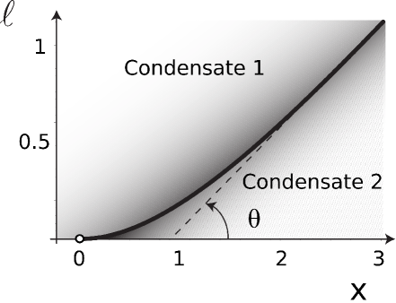
Figure 14: Cross-section perpendicular to the three-phase contact line where phases $1$, $2$ and the wall meet. Depicted is the interface displacement $\ell(x)$ in units of $10\,\xi_{{}_{c}}$ against the coordinate position $x$ in units of $\xi_{{}_{c}}$ for a $1$-$2$ interface which is incident on a hard wall and for an interface potential which is of the form $V(\ell)=\mathcal{S}\,e^{-0.1\,\ell/\xi_{{}_{c}}}$. For this calculation the ratio $-\mathcal{S}/\gamma_{12}$ equals 0.2. The interface meets the wall at $x=0$ (open circle) tangentially with zero slope and $\ell(x)\propto x^{2}$ for small $x>0$ (while $\ell(x)=0$ for $x<0$).

We focus on a three-phase contact line the cross-section of which is shown in Fig. 14. The line is centered about $x=0$ and $\ell=0$ ($\ell=0$ coincides with the surface of the optical hard wall) and runs along the $y$-direction (perpendicular to the figure). The interface displacement $\ell(x)$ has translational symmetry in the $y$-direction. Note that the shape of $\ell(x)$ displays a monotically increasing slope. This feature would be typical for a transition zone that corresponds to the approach to an ordinary critical wetting transition rather than a first-order wetting transition. Upon approach of an ordinary first-order wetting transition a transition zone with an inflection point would be expected indekeu1992 . This illustrates once again the extraordinary character of the wetting transition in this model of adsorbed BEC mixtures.

According to the interface displacement model (IDM) indekeu1992 ; dobbs , the line tension $\tau$ is the following functional of the interface displacement $\ell(x)$, at bulk two-phase coexistence,

$$\tau[\ell]= \int_{{}_{-\infty}}^{{}_{\infty}}\text{d}x\,\left[\gamma_{{}_{12}}\left[\sqrt{1+\ell_{{}_{x}}^{2}(x)}-1\right]\right.$$

$$+V(\ell(x))-\mathcal{S}+c(x)\Big{]}.$$ (38)

where $\ell_{{}_{x}}=\text{d}\ell(x)/\text{d}x$ and the piecewise constant $c(x)$ is such that the integrand vanishes at large values of $x$. Note that the $V(\ell)$ used in indekeu1992 ; dobbs is shifted with respect to our $V(\ell)$ by a constant equal to the spreading coefficient $S$. The first term in (VII) measures the excess energy per unit length due to the surface curvature close to the three-phase contact line. By a minimization procedure, one derives the relevant Euler-Lagrange equation and associated constant of the motion. One finds that the equilibrium (or optimal) $\ell(x)$ starts from zero, at, say $x=0$, with zero slope and finite second derivative, as shown in Fig. 14. Note that $\ell(x)=0$ for all $x<0$ (there is no microscopic adsorbed film of condensate 2 in this region). The line tension functional evaluated in this optimal profile provides the equilibrium line tension and can be written as the following integral dobbs :

$$\tau=\sqrt{2\gamma_{{}_{12}}}\int_{{}_{0}}^{{}_{\infty}}\text{d}\ell\, \left[\sqrt{(V(\ell)-\mathcal{S})\left(1-\frac{V(\ell)-\mathcal{S}}{2\gamma_{{}_{12}}}\right)}\right.$$

$$\quad\left.-\sqrt{-\mathcal{S}\left(1+\frac{\mathcal{S}}{2\gamma_{{}_{12}}}\right)}\right]$$ (39)

The validity of the use of the IDM for the purpose of calculating the properties of the three-phase contact line is determined by the requirement that $\ell(x)$ be slowly varying with $x$. Indeed, the $V(\ell)$ that is employed is a quantity that is a priori calculated for a uniform thickness $\ell$, not a spatially varying one. Nevertheless, extending it to a spatially varying function $V(\ell(x))$, one may hope to get a reasonable approximation for inhomogeneous configurations such as those we are interested in here. However, for contact angles that are not small, and certainly for $\theta\approx\pi/2$, the gradient $d\ell/dx$ is too large (and even diverges) for this model to be reliable and unphysical features should be expected. A discussion of some of the artifacts that may result can be found in dobbs .

The interface potentials as we found here in the GP theory, were all, except for one, of the typical form, asymptotically for $\ell\rightarrow\infty$,

$$V_{\rm typ}(\ell)=\mathcal{S}\,e^{-\ell/\xi_{{}_{c}}},$$ (40)

for partial wetting states ($\mathcal{S}\leq 0$) at two-phase coexistence. We will take this $V_{\rm typ}(\ell)$ as our model interface potential in what follows and attempt to determine the corresponding line tension and interface displacement as accurately as possible, within the IDM and also beyond the IDM by means of a conjecture based on symmetry and analyticity considerations.

Within the IDM, substitution of (40) in (VII) brings us to the analytic expression for the line tension:

$$\tau=\frac{\gamma_{{}_{12}}\xi_{{}_{c}}}{2} \left[(2\varsigma-1)(2\text{arcsin}[2\varsigma-1]+\pi)\right.$$

$$\quad\left.+4\sqrt{\varsigma(1-\varsigma)}(\ln[4(1-\varsigma)]-1)\right].$$ (41)

where $2\varsigma=-\mathcal{S}/\gamma_{{}_{12}}=1-\cos\theta$ with $\theta$ the angle at which the asymptote (for $x\rightarrow\infty$) to the wedge is incident on the wall (see the dashed line in Fig. 14).

This expression for $\tau$ is displayed in Fig. 15 as the solid line. Note that the model is “mirror” symmetric about $\theta=\pi/2$ (wetting/drying symmetry) and all properties at $\theta$ are identical to those at $\pi-\theta$ provided the roles of phases (and species) 1 and 2 are interchanged. This explains the presence of two solid lines, each of which is the supplement of the other. Since the IDM is most reliable for weakly varying $\ell(x)$, the reliable parts are those in black and the extensions that do not correspond to the physically stable solutions are in gray. The singularity at the crossing point $\theta=\pi/2$ is an artifact of the IDM. There is no physical singularity at the “neutral” point at which there is no preferential adsorption of one of the phases. On the other hand, the singularities at $\theta=0$ (and $\pi$) are physical and correspond to the wetting (and drying) phase transitions. Before we turn to those in more detail we point out yet another interesting fact.

An often used simplification of the IDM consist of expanding the square root in (VII) to first order in the gradient squared, thereby explicitly acknowledging that the model is meant to serve (only) for weakly varying $\ell(x)$. This is the so-named gradient-squared approximation of the IDM. At the level of (VII) one easily verifies that the gradient-squared approximation amounts to reducing the integrand in (VII) to $\sqrt{V(\ell)-\mathcal{S}}-\sqrt{-\mathcal{S}}$. In this approximation the analytic result for $\tau$ is the following simple expression

$$\tau=-2\sqrt{2}\,(1-\ln 2)\,\gamma_{{}_{12}}\xi_{{}_{c}}\,\sqrt{1-\cos\theta},$$ (42)

This simplification of (VII), together with its symmetric supplement, is displayed as the dashed lines in Fig. 15. While (42) is expected to lose accuracy more rapidly than (VII) upon increasing $\theta$ from zero, both are expected to be equally precise for small $\theta$ and indeed the asymptotic forms of (42) and (VII) approaching wetting are coincident. Specifically, $\tau$ approaches zero with a square-root singularity in the variable $1-\cos\theta$ (see Fig. 15). Consequently, approaching complete wetting, for $\theta\rightarrow 0$, we find that the line tension is asymptotically equal to

$$\tau\sim-2\,(1-\ln 2)\,\gamma_{{}_{12}}\xi_{{}_{c}}\,\theta,$$ (43)

and thus $\tau$ at wetting approaches zero from negative values.

This result is surprising because it is reminiscent of the behavior of the line tension close to critical wetting in systems with short-range forces (i.e., exponentially decaying $V(\ell)$) in a standard mean-field theory indekeu1992 . Since we are dealing with a wetting transition that is not critical but of first order, $\tau$ is expected to attain a non-zero and finite positive value, also from below, at wetting indekeu1992 . The behavior of the line tension at wetting depends, in mean-field theory, mainly on two characteristics. One is the order of the transition and the other is the range of the forces. Beyond mean-field theory there are fluctuation effects. For a review see indekeu4 .

We conclude that the line tension for adsorbed BEC mixtures displays a hybrid character, which is caused by the extraordinary absence of a barrier in the interface potential $V(\ell)$. The absence of a barrier implies that for $\theta\rightarrow 0$ there is no transition zone which builds up in $\ell(x)$ between zero thickness and a macroscopic (infinite) thickness. Instead, a completely flat profile $\ell(x)$ results. Note that we cannot exclude that physically a transition zone at first-order wetting may still exist in this system, but an interface displacement model based on $V(\ell)$ cannot capture it.

The results for $\tau$ obtained within the IDM, in gradient-squared approximation, (42), and beyond this approximation, (VII), suggest a conjecture for the exact solution for $\tau$ within GP theory and for the simple choice of interface potential given by (40), without correction terms that become important at small $\ell$ and would modify also the line tension results quantitatively. This conjecture is based on three assumptions: i) there is nothing physically special about $\theta=\pi/2$ (obtained for $\xi_{{}_{1}}=\xi_{{}_{2}}$) and $\tau$ must be smooth (i.e., analytic) in that vicinity, ii) the $\theta\rightleftharpoons\pi-\theta$ symmetry must be respected, and iii) the asymptotic behavior near wetting (and drying) established with the help of the IDM calculations must be preserved in detail. The simplest function which satisfies i)-iii) is:

$$\tau_{\rm conj}=-2\,(1-\ln 2)\,\gamma_{{}_{12}}\xi_{{}_{c}}\,\sin\theta,$$ (44)

and it is displayed by the dash-dotted line in gray in Fig. 15. Perhaps it is possible to verify this conjecture (to a decisive extent) by designing an exact calculation of $\tau$ right at $\theta=\pi/2$ in GP theory.

Let us now return to the IDM results and close this section with some remarks. While the expression (VII) is general and displays that $\tau$ is essentially a numerical factor times the interfacial tension multiplied by a characteristic surface-related length, it is possible in special cases (cf. the different regimes we studied) to obtain an explicit dependence on other characteristic lengths and on the interaction strength in our system. For example, in Sect. VI.4, we considered the case $\xi_{{}_{2}}/\xi_{{}_{1}}\rightarrow 0$ and $K\rightarrow\infty$ while $[\xi_{{}_{2}}/\xi_{{}_{1}}]\sqrt{K}$ was of order unity. We analyzed numerically the length scale of exponential decay of the interface potential, see (29), and the result was shown in Fig. 11. For the partial wetting regime, i.e., when $[\xi_{{}_{2}}/\xi_{{}_{1}}]\sqrt{K}>\sqrt{2}/3$, we found that $\xi_{{}_{c}}$ goes over from the value $\xi_{{}_{2}}/2$ to $\xi_{{}_{1}}/(2\sqrt{K})$ upon varying $[\xi_{{}_{2}}/\xi_{{}_{1}}]\sqrt{K}$. The dependence of the line tension on $\xi_{{}_{1}}$, $\xi_{{}_{2}}$ and $K$ therefore obeys:

$$\tau\propto P_{{}_{1}}\xi_{{}_{1}}\xi_{{}_{c}},$$ (45)

with a proportionality factor of order unity, and where we used that $\gamma_{{}_{12}}\approx P_{{}_{1}}\xi_{{}_{1}}$ and where the value of $\xi_{{}_{c}}$ is plotted in Fig.11. Note that $\tau$ scales as $1/\sqrt{K}$ and is therefore small.

We consider now the case of weak segregation (see Sect. VI.5), i.e., when $0<\xi_{{}_{1}}/\xi_{{}_{2}}-1\ll 1$ and $0<K-1\ll 1$, for which (VI.5) expresses the exact interface potential, to leading order for large $\ell$. At PW or when $2\sqrt{2}[\xi_{{}_{1}}/\xi_{{}_{2}}-1]/3<\sqrt{K-1}$, we found that

$$\cos\theta=\frac{2\sqrt{2}}{3}\frac{[\xi_{{}_{1}}/\xi_{{}_{2}}-1]}{\sqrt{K-1}},\quad\xi_{{}_{c}}=\frac{\xi_{{}_{2}}}{2\sqrt{K-1}},$$ (46)

since $\gamma_{{}_{12}}=2P_{{}_{1}}\xi_{{}_{2}}\sqrt{K-1}$.

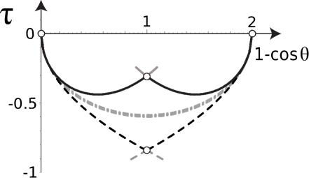
Figure 15: The line tension $\tau$ in units of $\gamma_{{}_{12}}\xi_{{}_{c}}$ versus $1-\cos\theta$, where $\theta$ is the interface inclination angle defined asymptotically, far from the three-phase contact line (i.e., the contact angle as predicted by Young’s law). The lower curves (dashed lines) correspond to the gradient-squared approximation within the IDM. The upper curves (solid lines) correspond to the full IDM calculations. For both approaches, the physically stable part is in black (the extension in gray). The smooth curve (dash-dotted in gray), which runs in between the stable parts of the IDM curves, corresponds to the conjecture (44) for the exact line tension in GP theory consistent with the typical interface potential (40).

VIII Conclusion

We established the interface potential $V(\ell)$ for binary mixtures of Bose-Einstein condensates near a hard wall. The interface potential relates a configuration of adsorbed film thickness $\ell$ of species $2$ to its excess grand potential per unit area such that the equilibrium thickness is the value which minimizes the potential. Generally, we find for large $\ell$, $V(\ell)=h\ell+Ae^{-\ell/\xi_{{}_{c}}}+\ldots$ where $h$ is the bulk field. At two-phase coexistence ($h=0$), the leading exponential decay dominates the entire $V(\ell)$. There is no barrier (contrary to what happens in other models where the next-to-leading terms may be relevant, too). When $A$ is positive, complete wetting (CW) occurs whereas partial wetting (PW) is induced by a negative $A$.

We distinguish the following regimes (when $h=0$) footnote8 :

1. strong healing length asymmetry $\xi_{{}_{2}}\ll\xi_{{}_{1}}$: CW and $\xi_{{}_{c}}=\xi_{{}_{1}}/(2\sqrt{K+1})$.

2. strong healing length asymmetry $\xi_{{}_{1}}\ll\xi_{{}_{2}}$: PW and $\xi_{{}_{c}}=\xi_{{}_{2}}/2$.

3. Strong segregation $1/K=0$: PW and $\xi_{{}_{c}}=\xi_{{}_{2}}/\sqrt{2}$.

4. Both strong segregation $1/K\ll 1$ and strong healing length asymmetry $\xi_{{}_{2}}\ll\xi_{{}_{1}}$:

   1. PW and $\xi_{{}_{c}}=\xi_{{}_{2}}/\sqrt{2}$ for $[[\xi_{{}_{2}}/\xi_{{}_{1}}]\sqrt{K}]^{-1}\lesssim 1$.

   2. transition from PW to CW and $\xi_{{}_{c}}=\xi_{{}_{1}}/(2\sqrt{K+1})$ for $[[\xi_{{}_{2}}/\xi_{{}_{1}}]\sqrt{K}]^{-1}\gtrsim 1$.

5. Weak segregation $0<K-1\ll 1$ and $0<\xi_{{}_{1}}/\xi_{{}_{2}}-1\ll 1$: transition from PW to CW and $\xi_{{}_{c}}=\xi_{{}_{2}}/\sqrt{K-1}$.

For the cases $4$ and $5$, the transition from PW to CW is mediated by a completely flat interface potential, that is, $V(\ell)=0$ for all $\ell$. This observation explains several earlier reported features of the extraordinary wetting (and prewetting) phase transition in this system. Of particular interest is case $5$ for which we obtained an analytical expression of the full interface potential (58), the leading term of which, for large $\ell$, was used as a typical model interface potential for calculating the line tension of a three-phase contact line where the 1-2 interface meets the wall.

The calculation of the line tension represents the most important physical advance reported here. The use of the IDM has allowed us to calculate properties of the inhomogeneous three-phase contact line based on the knowledge of the $V(\ell)$ calculated for homogeneous states. The first of these properties is the interface displacement profile $\ell(x)$ for partial wetting states. Close to wetting these profiles are akin to those normally expected near a critical wetting transition, in spite of the fact that the wetting transition here is of first order. The second property is the line tension $\tau$ for which we have analytic results from the IDM, as well as an analytic conjecture that satisfies all physical requirements for arbitrary contact angle $0<\theta<\pi$ and captures the precise singularity at wetting (or drying).

The fact that the line tension is maximal at wetting is in accord with the predictions from and expectations raised by other models and theories of the line tension indekeu4 . However, the fact that $\tau$ approaches zero at wetting (from negative values) and the precise linear dependence on $\theta$ with which it does so, is reminiscent of a mean-field critical wetting transition (for short-range forces) rather than a first-order one. This hybrid character of $\tau$ (reinforced by the fact that the boundary tension along prewetting is zero) is explained by the fully flat barrierless $V(\ell)$ at wetting, which we calculated in this work.

IX Acknowledgements

The authors acknowledge partial support by Projects Nos. FWO G.0115.06, GOA/2004/02, the KU Leuven Research Fund and useful discussions with Achilleas Lazarides and Dmitry Tatyanenko, all at the early stages of this research.

X Appendix

What follows are the solutions for the interface potentials as closed-form integral expressions wherein the parameter $\eta$ must be eliminated to obtain the relation between $V(\ell)$ and $\ell$. Note that one may find (rather elaborate) analytic expressions in terms of hyperbolic integrals for the expressions which follow.

1. Define first the functional and functions:

   $$\widehat{\mathcal{Z}}_{{}_{0}}(A,\, B;[C(r),\,D(r)])\equiv\int_{\sqrt{A}}^{\sqrt{B}}\frac{\text{d}r}{\sqrt{D(r)}}\left(D(r)+C(r)\right),$$ (47a)

   $$\mathcal{Z}_{{}_{1}}(r) \equiv 1-2\eta r^{2}+r^{4},$$ (47b)

   $$\mathcal{Z}_{{}_{2}}(r) \equiv 1-\eta^{2}+2r^{2}(\eta K-1)+(1-K^{2})r^{4},$$ (47c)

   $$\mathcal{Z}_{{}_{3}}(r) \equiv 2r^{2}(K-\eta)+(1-K^{2})r^{4},$$ (47d)

   $$\mathcal{Z}_{{}_{4}}(r) \equiv 1-2r^{2}+r^{4},$$ (47e)

   $$\mathcal{Z}_{{}_{5}}(r) \equiv r^{2}(\eta-1),$$ (47f)

   $$\mathcal{Z}_{{}_{6}}(r) \equiv r^{2}-\mathcal{Z}_{{}_{3}}(r),$$ (47g)

   $$\mathcal{Z}_{{}_{7}}(r) \equiv r^{2}-\mathcal{Z}_{{}_{1}}(r),$$ (47h)

   $$\mathcal{Z}_{{}_{8}}(r) \equiv(\eta-1)(\eta-Kr^{2}),$$ (47i)

   $$\mathcal{Z}_{{}_{9}}(r) \equiv\eta-Kr^{2}-\mathcal{Z}_{{}_{2}}(r).$$ (47j)

2. We briefly explain now how to obtain the interface potential for the case $\xi_{{}_{2}}/\xi_{{}_{1}}=0$, as treated in section VI.1. The potentials of section VI.2 and VI.3 are given below and can be obtained in a similar fashion. Looking at Fig. 4, one sees that one can split the path of the densities $(\psi_{{}_{1}},\psi_{{}_{2}})$ into three parts. Since $\xi_{{}_{2}}/\xi_{{}_{1}}=0$, there is no energy contained in the vertical path with $\psi_{{}_{1}}=0$. The equations of motion for the curved path are given in (17) for which the conservation of energy yields:

   $$\xi_{{}_{1}}^{2}\dot{\psi^{2}_{{}_{1}}} =\frac{1-\eta^{2}}{2}+\psi_{{}_{1}}^{2}(\eta K-1)+\frac{1-K^{2}}{2}\psi_{{}_{1}}^{4}.$$ (48)

   Further, the horizontal path starts in ($\sqrt{K/\eta},\,0$) and arrives in $(1,\,0)$ as depicted in Fig. 4. The equations of motion are there governed by (18) with the following conservation of energy:

   $$\xi_{{}_{1}}^{2}\dot{\psi^{2}_{{}_{1}}}=\frac{1}{2}-\psi_{{}_{1}}^{2}+\psi_{{}_{1}}^{4}.$$ (49)

   Writing out expression (13), we get

   $$\frac{V(\ell)+\gamma_{{}_{0}}-h\ell}{2P_{{}_{1}}\xi_{{}_{1}}} =\int_{{}_{0}}^{{}_{\infty}}\text{d}z\,\left[2\xi_{{}_{1}}^{2}\dot{\psi_{{}_{1}}^{2}}+(\eta-1)\psi_{{}_{2}}^{2}\right].$$ (50)

   Splitting the integrals into the parts $[0,z_{{}_{0}}]$ and $[z_{{}_{0}},\infty]$, using the transformation $\text{d}z=\text{d}\psi_{{}_{1}}/\dot{\psi}_{{}_{1}}$, combined with the conservation laws (48) and (49), we then find

   $$\frac{V(\ell)+\gamma_{{}_{0}}-h\ell}{2\sqrt{2}P_{{}_{1}}\xi_{{}_{1}}}= \widehat{\mathcal{Z}}_{{}_{0}}\left(\,\eta/K,\,1;[0,\mathcal{Z}_{{}_{4}}(r)]\right)$$

   $$+\widehat{\mathcal{Z}}_{{}_{0}}\left(0,\,\eta/K;\left[\mathcal{Z}_{{}_{8}},\,\mathcal{Z}_{{}_{2}}(r)\right]\right),$$ (51)

   with the functions $\mathcal{Z}_{{}_{8}}$, $\mathcal{Z}_{{}_{2}}$ and $\mathcal{Z}_{{}_{4}}$ defined in (47). We eliminate the multiplier $\eta<1$ by writing:

   $$\frac{\ell}{\xi_{{}_{1}}}=\sqrt{2}\widehat{\mathcal{Z}}_{{}_{0}} \left(0,\,\eta/K;[\mathcal{Z}_{{}_{9}}(r),\,\mathcal{Z}_{{}_{2}}(r)]\right).$$ (52)

   The coefficient $\overline{A}_{{}_{1}}$ in (19) is:

   $$\overline{A}_{{}_{1}}=\frac{128\sqrt{2}}{3}\frac{(2K+1)(K-1)^{3}}{K^{3/2}(K+1)^{2}}$$ (53)

   $$\times\left[\frac{\sqrt{2K}+\sqrt{K-1}}{\sqrt{2K}-\sqrt{K-1}}\right]\exp\left[4K\left(1-\sqrt{\frac{K-1}{2K}}\right)\right].$$

3. For the wall-adsorbed states in the case of $\xi_{{}_{1}}/\xi_{{}_{2}}=0$, the interface potential is found to be a solution of the following two Eqs. with $\eta>1$:

   $$\frac{V(\ell)+\gamma_{{}_{0}}-h\ell}{2\sqrt{2}P_{{}_{1}}\xi_{{}_{2}}}=\widehat{\mathcal{Z}}_{{}_{0}}\left(0,\,1/K;[\mathcal{Z}_{{}_{5}}(r),\,\mathcal{Z}_{{}_{3}}(r)]\right)$$ (54a)

   $$\quad\quad\quad\quad+\widehat{\mathcal{Z}}_{{}_{0}}\left(0,\,\eta-\sqrt{\eta^{2}-1};[\mathcal{Z}_{{}_{5}}(r),\,\mathcal{Z}_{{}_{1}}(r)]\right)$$

   $$\quad\quad\quad\quad+\widehat{\mathcal{Z}}_{{}_{0}}\left(1/K,\,\eta-\sqrt{\eta^{2}-1};[\mathcal{Z}_{{}_{5}}(r),\,\mathcal{Z}_{{}_{1}}(r)]\right),$$

   $$\frac{\ell}{\xi_{{}_{2}}}=\sqrt{2}\,\widehat{\mathcal{Z}}_{{}_{0}}\left(0,\,1/K;[\mathcal{Z}_{{}_{6}}(r),\,\mathcal{Z}_{{}_{3}}(r)]\right)$$ (54b)

   $$\quad\quad\quad+\sqrt{2}\,\widehat{\mathcal{Z}}_{{}_{0}}\left(1/K,\,\eta-\sqrt{\eta^{2}-1};[\mathcal{Z}_{{}_{7}}(r),\,\mathcal{Z}_{{}_{1}}(r)]\right)$$

   $$\quad\quad\quad+\sqrt{2}\,\widehat{\mathcal{Z}}_{{}_{0}}\left(0,\,\eta-\sqrt{\eta^{2}-1};[\mathcal{Z}_{{}_{7}}(r),\,\mathcal{Z}_{{}_{1}}(r)]\right).$$

4. For the bulk states with $\xi_{{}_{1}}/\xi_{{}_{2}}=0$, we must distinguish two cases. First of all, when the multiplier $\eta$ takes the values $(1+K^{2})/(2K)<\eta<K$, we have:

   $$\frac{V(\ell)+\gamma_{{}_{0}}-h\ell}{4\sqrt{2}P_{{}_{1}}\xi_{{}_{2}}}=\,\widehat{\mathcal{Z}}_{{}_{0}}\left(0,\,\frac{2(K-\eta)}{K^{2}-1};[\mathcal{Z}_{{}_{5}}(r),\,\mathcal{Z}_{{}_{3}}(r)]\right),$$ (55a)

   $$\frac{\ell}{\xi_{{}_{2}}}=2\sqrt{2}\,\widehat{\mathcal{Z}}_{{}_{0}}\left(0,\,\frac{2(K-\eta)}{K^{2}-1};[\mathcal{Z}_{{}_{6}}(r),\,\mathcal{Z}_{{}_{3}}(r)]\right).$$ (55b)

   Secondly, when $1<\eta<(1+K^{2})/(2K)$, we have:

   $$\frac{V(\ell)+\gamma_{{}_{0}}-h\ell}{4\sqrt{2}P_{{}_{1}}\xi_{{}_{2}}}=\,\widehat{\mathcal{Z}}_{{}_{0}}\left(0,\,1/K;[\mathcal{Z}_{{}_{5}}(r),\,\mathcal{Z}_{{}_{3}}(r)]\right)$$ (56a)

   $$+\,\widehat{\mathcal{Z}}_{{}_{0}}\left(1/K,\,\eta-\sqrt{\eta^{2}-1};[\mathcal{Z}_{{}_{5}}(r),\,\mathcal{Z}_{{}_{1}}(r)]\right),$$

   $$\frac{\ell}{\xi_{{}_{2}}}=2\sqrt{2}\,\widehat{\mathcal{Z}}_{{}_{0}}\left(0,\,1/K;[\mathcal{Z}_{{}_{6}}(r),\,\mathcal{Z}_{{}_{3}}(r)]\right)$$ (56b)

   $$+2\sqrt{2}\,\widehat{\mathcal{Z}}_{{}_{0}}\left(1/K,\,\eta-\sqrt{\eta^{2}-1};[\mathcal{Z}_{{}_{7}}(r),\,\mathcal{Z}_{{}_{1}}(r)]\right).$$

5. When $1/K=0$, the interface potential is found through a solution of the following two Eqs. with $\eta>1$:

   $$\frac{V(\ell)+\gamma_{{}_{0}}-h\ell}{4\sqrt{2}P_{{}_{1}}\xi_{{}_{2}}}=\,\widehat{\mathcal{Z}}_{{}_{0}}\left(0,\eta-\sqrt{\eta^{2}-1};[\mathcal{Z}_{{}_{5}}(r),\,\mathcal{Z}_{{}_{1}}(r)]\right),$$ (57a)

   $$\frac{\ell}{\xi_{{}_{2}}}=2\sqrt{2}\widehat{\mathcal{Z}}_{{}_{0}}\left(0,\eta-\sqrt{\eta^{2}-1};[\mathcal{Z}_{{}_{6}}(r),\,\mathcal{Z}_{{}_{1}}(r)]\right).$$ (57b)

6. The exact interface potential in the case $0<K-1\ll 1$ and $0<\xi_{{}_{1}}/\xi_{{}_{2}}-1\ll 1$ is

   $$V(\ell)=\frac{1}{\sqrt{2}}\left[\frac{2\sqrt{2}(\xi_{{}_{1}}/\xi_{{}_{2}}-1)}{3\sqrt{K-1}}-1\right]\times$$ (58)

   $$\text{LambertW}\left(-2\sqrt{2}\sqrt{K-1}\,e^{-2\sqrt{K-1}\,(\ell/\xi_{{}_{2}}+\sqrt{2})}\right),$$

   where LambertW$(x)$ is the solution $y(x)$ to the equation $y(x)e^{y(x)}=x$.

References

- (1) L.P. Pitaevskii and S. Stringari, Bose-Einstein Condensation, Clarendon Press, Oxford, 2003.
- (2) S. Inouye, M.R. Andrews, J. Stenger, H.-J. Miesner, D.M. Stamper-Kurn and W. Ketterle, Observation of Feshbach resonances in a Bose–Einstein condensate, Nature (London) 392, 151 (1998).
- (3) C.A. Stan, M.W. Zwierlein, C.H. Schunck, S.M.F. Raupach and W. Ketterle, Observation of Feshbach resonances between two different atomic species, Phys. Rev. Lett. 93, 143001 (2004).
- (4) S.B. Papp and C.E. Wieman, Observation of heteronuclear Feshbach molecules from a Rb 85–Rb 87 gas, Phys. Rev. Lett. 97, 180404 (2006).
- (5) D. Rychtarik, B. Engeser, H.-C. Nägerl and R. Grimm, Two-dimensional Bose-Einstein condensate in an optical surface trap, Phys. Rev. Lett. 92, 173003 (2004).
- (6) H. Perrin, Y. Colombe, B. Mercier, V. Lorent and C. Henkel, A Bose–Einstein condensate bouncing off a rough mirror, J. Phys.: Conf. Ser. 19, 151 (2005); Y. Colombe, B. Mercier, H. Perrin, V. Lorent, Diffraction of a Bose-Einstein condensate in the time domain, Phys. Rev. A 72, 061601(R) (2005).
- (7) N. Navon, R.P. Smith and Z. Hadzibabic, Quantum gases in optical boxes, Nat. Phys. 17, 1334 (2021).
- (8) A.L. Gaunt, T.F. Schmidutz, I. Gotlibovych, R.P. Smith, and Z. Hadzibabic, Bose-Einstein condensation of atoms in a uniform potential, Phys. Rev. Lett. 110, 200406 (2013).
- (9) B. Mukherjee, Z. Yan, P.B. Patel, Z. Hadzibabic, T. Yefsah, J. Struck and M.W. Zwierlein, Homogeneous atomic Fermi gases, Phys. Rev. Lett. 118, 123401 (2017).
- (10) G. Modugno, M. Modugno, F. Riboli, G. Roati and M. Inguscio, Two atomic species superfluid, Phys. Rev. Lett. 89, 190404 (2002).
- (11) H.-J. Miesner, D.M. Stamper-Kurn, J. Stenger, S. Inouye, A.P. Chikkatur and W. Ketterle, Observation of metastable states in spinor Bose-Einstein condensates, Phys. Rev. Lett. 82, 2228 (1999).
- (12) C.J. Myatt, E.A. Burt, R.W. Ghrist, E.A. Cornell and C.E. Wieman, Production of two overlapping Bose-Einstein condensates by sympathetic cooling, Phys. Rev. Lett. 78, 586 (1997).
- (13) D.M. Stamper-Kurn, H.-J. Miesner, A.P. Chikkatur, S. Inouye, J. Stenger and W. Ketterle, Quantum tunneling across spin domains in a Bose-Einstein condensate, Phys. Rev. Lett. 83, 661 (1999).
- (14) D.S. Hall, M.R. Matthews, J.R. Ensher, C.E. Wieman and E.A. Cornell, Dynamics of component separation in a binary mixture of Bose-Einstein condensates, Phys. Rev. Lett. 81, 1539 (1998).
- (15) M.R. Matthews, B.P. Anderson, P.C. Haljan, D.S. Hall, C.E. Wieman and E.A. Cornell, Vortices in a Bose-Einstein condensate, Phys. Rev. Lett. 83, 2498 (1999).
- (16) D. J. McCarron, H. W. Cho, D. L. Jenkin, M. P. Köppinger and S. L. Cornish, Dual-species Bose-Einstein condensate of Rb 87 and Cs 133, Phys. Rev. A 84, 011603(R) (2011).
- (17) S. Tojo, Y. Taguchi, Y. Masuyama, T. Hayashi, H. Saito and T. Hirano, Controlling phase separation of binary Bose-Einstein condensates via mixed-spin-channel Feshbach resonance, Phys. Rev. A 82, 033609 (2010).
- (18) P. A. Altin, N. P. Robins, D. Döring, J. E. Debs, R. Poldy, C. Figl and J. D. Close, Rb 85 tunable-interaction Bose–Einstein condensate machine, Rev. Sci. Instrum. 81, 063103 (2010).
- (19) S. Papp, J. Pino and C. Wieman, Tunable miscibility in a dual-species Bose-Einstein condensate, Phys. Rev. Lett. 101, 040402 (2008).
- (20) K.E. Wilson, A. Guttridge, J. Segal and S.L. Cornish, Quantum degenerate mixtures of Cs and Yb, Phys. Rev. A, 103, 033306 (2021).
- (21) A. Burchianti, C. D’Errico, S. Rosi, A. Simoni, M. Modugno, C. Fort and F. Minardi, Dual-species Bose-Einstein condensate of K 41 and Rb 87 in a hybrid trap, Phys. Rev. A 98, 063616 (2018).
- (22) K.L. Lee, N.B. Jørgensen, L.J. Wacker, M.G. Skou, K.T. Skalmstang, J.J. Arlt and N.P. Proukakis, Time-of-flight expansion of binary Bose–Einstein condensates at finite temperature, New J. Phys. 20, 053004 (2018).
- (23) F. Wang, X. Li, D. Xiong, D. Wang, A double species 23Na and 87Rb Bose–Einstein condensate with tunable miscibility via an interspecies Feshbach resonance, J. Phys. B: At. Mol. Opt. Phys. 49, 015302 (2015).
- (24) R.S. Lous, I. Fritsche, M. Jag, F. Lehmann, E. Kirilov, B. Huang and R. Grimm, Probing the interface of a phase-separated state in a repulsive bose-fermi mixture, Phys. Rev. Lett. 120, 243403 (2018).
- (25) B. Van Schaeybroeck and A. Lazarides, Normal-superfluid interface scattering for polarized fermion gases, Phys. Rev. Lett. 98, 170402 (2007).
- (26) P.T. Grochowski, T. Karpiuk, M. Brewczyk, K. Rzazewski, Breathing mode of a Bose-Einstein condensate immersed in a Fermi sea, Phys. Rev. Lett. 125, 103401 (2020).
- (27) V.P. Ruban, Capillary flotation in a system of two immiscible Bose-Einstein condensates, JETP Lett. 113, 814 (2021).
- (28) K. Jimbo and H. Saito, Surfactant behavior in three-component Bose-Einstein condensates, Phys. Rev. A 103, 063323 (2021).
- (29) J.O. Indekeu, C.-Y. Lin, T.V. Nguyen, B. Van Schaeybroeck and T.H. Phat, Static interfacial properties of Bose-Einstein-condensate mixtures, Phys. Rev. A 91, 033615 (2015).
- (30) D.K. Maity, K. Mukherjee, S.I. Mistakidis, S. Das, P.G. Kevrekidis, S. Majumder and P. Schmelcher, Parametrically excited star-shaped patterns at the interface of binary Bose-Einstein condensates, Phys. Rev. A 102, 033320 (2020).
- (31) A. Balaž and A.I. Nicolin, Faraday waves in binary nonmiscible Bose-Einstein condensates, Phys. Rev. A 85, 023613 (2012).
- (32) J.O. Indekeu, N. Van Thu, C.-Y. Lin and T.H. Phat, Capillary-wave dynamics and interface structure modulation in binary Bose-Einstein condensate mixtures, Phys. Rev. A 97, 043605 (2018).
- (33) S. Pal, A. Roy and D. Angom, Collective modes in multicomponent condensates with anisotropy, J. Phys. B: At. Mol. Opt. Phys. 51, 085302 (2018).
- (34) J.W. Cahn, Critical point wetting, J. Chem. Phys. 66, 3667 (1977).
- (35) C. Ebner and W. F. Saam, New phase-transition phenomena in thin argon films, Phys. Rev. Lett. 38, 1486 (1977).
- (36) H. Nakanishi and M.E. Fisher, Multicriticality of wetting, prewetting, and surface transitions, Phys. Rev. Lett. 49, 1565 (1982).
- (37) K. Binder, D.P. Landau and M. Müller, Monte Carlo studies of wetting, interface localization and capillary condensation, J. Stat. Phys. 110, 1411 (2003).
- (38) P.-G. de Gennes, Wetting: statics and dynamics, Rev. Mod. Phys. 57, 827 (1985).
- (39) S. Dietrich, Wetting phenomena, in Phase Transitions and Critical Phenomena, edited by C. Domb and J.L. Lebowitz (Academic, London), Vol. 12, 1 (1988).
- (40) D. Bonn and D. Ross, Wetting transitions, Rep. Prog. Phys. 64, 1085 (2001).
- (41) J.O. Indekeu and B. Van Schaeybroeck, Extraordinary wetting phase diagram for mixtures of Bose-Einstein condensates, Phys. Rev. Lett. 93, 210402 (2004).
- (42) B. Van Schaeybroeck and J.O. Indekeu, Critical wetting, first-order wetting, and prewetting phase transitions in binary mixtures of Bose-Einstein condensates, Phys. Rev. A 91, 013626 (2015).
- (43) J.O. Indekeu, Wetting phase transitions and critical phenomena in condensed matter, Physica A 389, 4332 (2010).
- (44) J.O. Indekeu and J.M.J. van Leeuwen, Interface delocalization transition in type-I superconductors, Phys. Rev. Lett. 75, 1618 (1995).
- (45) J.O. Indekeu and J.M.J. van Leeuwen, Wetting, prewetting and surface transitions in type-I superconductors, Physica C 251, 290 (1995).
- (46) R. Blossey and J.O. Indekeu, Interface-potential approach to surface states in type-I superconductors, Phys. Rev. B 53, 8599 (1996).
- (47) C.J. Boulter and J.O. Indekeu, Analytic determination of the interface delocalization transition in low- superconductors, Physica C 271, 94 (1996).
- (48) J.M.J. van Leeuwen and E.H. Hauge, The effective interface potential for a superconducting layer, J. Stat. Phys. 87, 1335 (1997).
- (49) J.M.J. van Leeuwen and J.O. Indekeu, Interface potential for nucleation of a superconducting layer, Physica A 244, 426 (1997).
- (50) C.J. Boulter and J.O. Indekeu, Systematic smoothing of constrained interface profiles, Phys. Rev. E 56, 5734 (1997).
- (51) E. Brézin, B.I. Halperin and S. Leibler, Critical wetting in three dimensions, Phys. Rev. Lett. 50, 1387 (1983).
- (52) R. Lipowsky, Upper critical dimension for wetting in systems with long-range forces, Phys. Rev. Lett. 52, 1429 (1984).
- (53) R. Lipowsky, D.M. Kroll and R.K.P. Zia, Effective field theory for interface delocalization transitions, Phys. Rev. B 27, 4499 (1983).
- (54) R. Lipowsky, Critical effects at complete wetting, Phys. Rev. B 32, 1731 (1985).
- (55) R. Lipowsky and M.E. Fisher, Scaling regimes and functional renormalization for wetting transitions, Phys. Rev. B 36, 2126 (1987).
- (56) D. Bonn, J. Eggers, J. Indekeu, J. Meunier and E. Rolley, Wetting and spreading, Rev. Mod. Phys. 81, 739 (2009).
- (57) A.O. Parry and P. Swain, Physica A 250, 167 (1998).
- (58) A.O. Parry and C. Rascon, The trouble with critical wetting, J. Low Temp. Phys. 157, 149 (2009).
- (59) L. Schimmele, M. Napiorkowski and S. Dietrich, Conceptual aspects of line tensions, J. Chem. Phys. 127, 164715 (2007).
- (60) J.O. Indekeu, Line tension at wetting, Int. J. Mod. Phys. B 8, 309 (1994).
- (61) B. Van Schaeybroeck, Interfaces and wetting in ultracold gases, PhD thesis, KU Leuven (2007).
- (62) A.L. Fetter and J.D. Walecka, Quantum theory of many-particle systems, McGraw Hill, Boston, 1971.
- (63) P. Ao and S.T. Chui, Binary Bose-Einstein condensate mixtures in weakly and strongly segregated phases, Phys. Rev. A 58, 4836 (1998).
- (64) Three remarks can be made. 1) The system can also be seen as a one-particle system in two dimensions in which the particle has anisotropic mass. 2) Rotational symmetry of the potential is only recovered for . 3) Minima of the excess energy correspond to maxima of the potential .
- (65) In what follows we draw -paths, rather than interface density profiles. Thereby, we gain the possibility of showing the potential in which the particles move, together with the influence of the parameters and . Showing the -paths is particularly useful when the system involves two largely different length scales (being the time scales in the dynamical approach). In that case, spatial density profiles are difficult to visualize.
- (66) E.H. Hauge, Landau theory of wetting in systems with a two-component order parameter, Phys. Rev. B 33, 3322 (1986).
- (67) K. Koga, J. O. Indekeu, and B. Widom, Infinite-order transitions in density-functional models of wetting, Phys. Rev. Lett. 104, 036101 (2010).
- (68) Therefore also, the healing length of species equals instead of .
- (69) The fact that length must be finite when and , and therefore , can be understood as follows. If indeed were to diverge at , for nonvanishing coefficients in front of the exponents, this would give rise to a constant interface potential. However, this is incompatible with the nonzero spreading coefficient.
- (70) B. Van Schaeybroeck, Interface tension of Bose-Einstein condensates, Phys. Rev. A 78, 023624 (2008). See also the Addendum, B. Van Schaeybroeck, Phys. Rev. A 80, 065601 (2009).
- (71) We were unable to prove this statement analytically. The difficulty is that, for a fixed value of the film thickness, the corresponding disjoining pressures of bulk-nucleated and wall-adsorbed states differ.
- (72) In fact, we first consider to be very small but nonzero so that some overlap between species and persists and thus expression (12) is still valid. Only then we take the limit .
- (73) C.J. Boulter and J.O. Indekeu, Accurate analytic expression for the surface tension of a type-I superconductor, Phys. Rev. B 54, 12407 (1996).
- (74) E.H. Hauge and M. Schick, Continuous and first-order wetting transition from the van der Waals theory of fluids, Phys. Rev. B 27, 4288 (1983).
- (75) It is unclear at this point whether the deviations around as seen in Fig. 11 are due to numerical errors or not.
- (76) B.A. Malomed, A.A. Nepomnyashchy and M. Tribelsky, Domain boundaries in convection patterns, Phys. Rev. A 42, 7244 (1990).
- (77) I.E. Mazets, Waves on an interface between two phase-separated Bose-Einstein condensates, Phys. Rev. A 65, 033618 (2002).
- (78) J.O. Indekeu, Line tension near the wetting transition: results from an interface displacement model, Physica A 183, 439 (1992).
- (79) H.T. Dobbs and J.O. Indekeu, Line tension at wetting: interface displacement model beyond the gradient-squared approximation, Physica A 201, 457 (1993).
- (80) Within the domain where the GP formalism is, to a good approximation, valid, the here obtained interface potential will remain as it is. Indeed, for small but nonzero absolute temperature and upon ignoring quantum fluctuations, thermal fluctuations will renormalize the interface potential; it is known that the corrections can be developed as a function of the parameter where is the decay length of the interface potential; a fluctuation-dominated regime arises when the parameter is of order unity or larger. For the system under consideration we find . Indeed, since is always larger than the healing length (take for simplicity that ), one finds that . However, we know that in the current experiments and such that pita . Therefore, at low temperature, thermal fluctuations of the interface are expected to alter the interface potentials which were obtained in this chapter, only weakly. As was proven in vanschaeybroeck , the finite-temperature corrections to the interfacial tension are small, except possibly for weak segregation.