Constraint energy minimizing generalized multiscale finite element method for inhomogeneous boundary value problems with high contrast coefficients

Abstract

In this article we develop the Constraint Energy Minimizing Generalized Multiscale Finite Element Method (CEM-GMsFEM) for elliptic partial differential equations with inhomogeneous Dirichlet, Neumann, and Robin boundary conditions, and the high contrast property emerges from the coefficients of elliptic operators and Robin boundary conditions. By careful construction of multiscale bases of the CEM-GMsFEM, we introduce two operators $\mathcal{D}^{m}$ and $\mathcal{N}^{m}$ which are used to handle inhomogeneous Dirichlet and Neumann boundary values and are also proved to converge independently of contrast ratios as enlarging oversampling regions. We provide a priori error estimate and show that oversampling layers are the key factor in controlling numerical errors. A series of experiments are conducted, and those results reflect the reliability of our methods even with high contrast ratios.

Keywords Constraint energy minimization  $\cdot$ multiscale finite element methods  $\cdot$ high contrast problems  $\cdot$ inhomogeneous boundary value problems

1 Introduction

Many practical problems drive us to study partial differential equations (PDE) with inhomogeneous coefficients. For example, Darcy’s law in inhomogeneous or even fractured media, elasticity systems in composite materials. When coefficients show special structures, such as periodicity and stochasticity, a great number of mathematical theories have been established Bensoussan et al. (2011); Dal Maso (1993); Jikov et al. (1994); Pankov (1997); Conca and Vanninathan (1997); Cioranescu and Donato (1999); Cioranescu et al. (2008); Tartar (2009); Shen (2018); Armstrong et al. (2019), which have been cornerstones of multiscale modeling and simulations. As for general inhomogeneous coefficients which are usually accompanied by high contrast channels, it has been viewed as a long-standing challenge for traditional methods. The reason is in two aspects: channelized structures require fine meshes which dramatically increase freedom degrees, and high contrast ratios deteriorate convergences of solvers for final linear systems.

To handle those problems, many multiscale computational methods have been developed since the 1990s. To name a few, multiscale finite element methods Hou and Wu (1997); Hou et al. (1999); Chen and Hou (2003); Efendiev and Hou (2009), Heterogeneous Multiscale Methods (HMM) E and Engquist (2003); E et al. (2005); Abdulle et al. (2012), variational multiscale methods Hughes (1995); Brezzi et al. (1997); Hughes and Sangalli (2007), generalized finite element methods Babuska and Lipton (2011); Babuška et al. (2020), Generalized Multiscale Finite Element Methods (GMsFEM) Efendiev et al. (2013); Chung et al. (2014, 2016), and Localized Orthogonal Decomposition (LOD) methods Må lqvist and Peterseim (2014); Henning and Må lqvist (2014); Altmann et al. (2021); Hellman and Må lqvist (2017); Må lqvist and Peterseim (2021). A universal thought in those methods (except HMMs) is encoding fine-scale information into basis functions of Finite Element Methods (FEM), then solving original problems on multiscale finite element spaces whose dimensions have been greatly reduced compared to default FEMs. We also notice that most existing literature in multiscale computational methods chooses homogeneous Dirichlet or Neumann Boundary Value Problems (BVP) as model problems to study convergence theories and conduct numerical experiments, while extensions of those methods to inhomogeneous BVPs are sometimes nontrivial (e.g., Henning and Må lqvist (2014)). Since solving inhomogeneous BVPs is a practical demand from the application side, it is necessary to examine the effectiveness of existing multiscale computational methods and extend them to complex BVPs.

This work is based on Constrained Energy Minimizing Generalized Multiscale Finite Element Methods (CEM-GMsFEM), which was originally proposed in Chung et al. (2018a) for high contrast problems and are applied to many applications Vasilyeva et al. (2019); Wang et al. (2021); Chung and Pun (2020); Chung et al. (2018a). Note that there are two versions of CEM-GMsFEMs proposed in Chung et al. (2018a), and we focus on the modified one—relaxed CEM-GMsFEM, which shows advantage both in theories and implementations. However, according to the construction of multiscale bases in CEM-GMsFEMs—solving energy minimizing problems on oversampling regions, either pressures or flow rates (terms from Darcy’s law) of basis functions vanish on boundaries, which implies that it cannot be directly utilized in inhomogeneous BVPs. Moreover, additional physical coefficients will be introduced in Robin boundary conditions, and those coefficients may also be high contrast. Those reasons lead us to reconsider how to apply CEM-GMsFEMs to inhomogeneous BVPs in high contrast settings.

There are many common points in CEM-GMsFEMs and LOD methods, for example, both rely on exponential decay properties of bases and need mesh size-dependent oversampling regions to achieve an optimal convergence rate. We emphasize that large oversampling regions are essential here because there are theoretical evidences that reveal high contrast is strongly related to nonlocality Bellieud and Bouchitté (1998); Briane (2002); Du et al. (2020) . The major difference is that CEM-GMsFEMs solve element-wise eigenvalue problems to obtain auxiliary spaces and projection operators (such an idea is originated from GMsFEMs Efendiev et al. (2013)), while LOD methods adopt quasi-interpolation operators, such as the Scott-Zhang operator Scott and Zhang (1990). Since eigenvalue problems have integrated coefficient information, exponential decay rates are now explicitly dependent on $\Lambda$, where $\Lambda$ is the minimal eigenvalue that the corresponding eigenvector is not included in auxiliary spaces. From numerical experiments, $\Lambda$ is quite stable with varying contrast ratios. A minor difference from implementations is that relaxed CEM-GMsFEMs deal with quadratic form minimization problems in constructing multiscale bases, while LOD methods need to solve saddle point problems.

The paper is organized as follows: in section 2, we introduce some preliminaries; in section 3, we present details of the methods, provide a rigorous analysis of numerical errors and extend the computational framework to inhomogeneous Robin BVPs; in section 4, we conduct a series of numerical experiments to verify accuracy of our methods in high contrast settings.

2 Preliminaries

Denote by $\Omega\subset\mathbb{R}^{d}$ ($d=2$ or $3$) a Lipschitz domain and $\mathbf{A}(x)\in L^{\infty}\left(\Omega;\mathbb{R}^{d\times d}\right)$ a matrix-valued function defined on $\Omega$, we consider the following model problem:

$$\left\{\begin{aligned} &-\operatorname{div}\left(\mathbf{A}\nabla u\right)=f\ &\text{in}\ \Omega,\\ &u=g\ &\text{on}\ {\Gamma_{\textnormal{D}}},\\ &\nu\cdot\mathbf{A}\nabla u=q\ &\text{on}\ {\Gamma_{\textnormal{N}}},\end{aligned}\right.$$ (1)

where $\nu$ stands for outward unit normal vectors to $\partial\Omega$, ${\Gamma_{\textnormal{D}}}$ and ${\Gamma_{\textnormal{N}}}$ are two nonempty disjointed parts of $\partial\Omega$. In this paper, we present the following assumptions for the model problem:

A1

There exist positive constants $0<A_{1}\leq A_{2}$ such that for a.e. $x\in\Omega$, $\mathbf{A}(x)$ is a positive define matrix with

$$A_{1}\leq\lambda_{\min}\left(\mathbf{A}(x)\right)\leq\lambda_{\max}\left(\mathbf{A}(x)\right)\leq A_{2}.$$

A2

The source term $f\in L^{2}(\Omega)$, the Dirichlet boundary value term $g\in H^{\frac{1}{2}}({\Gamma_{\textnormal{D}}})$ and the Neumann boundary value term $q\in L^{2}({\Gamma_{\textnormal{N}}})$.

We rewrite the inhomogeneous BVP eq. 1 in a variational form for designing computational methods: find a solution $u_{0}\in V=\left\{v\in H^{1}(\Omega):v=0\ \text{on}\ {\Gamma_{\textnormal{D}}}\right\}$ such that for all $v\in V$,

$$\int_{\Omega}\mathbf{A}\nabla u_{0}\cdot\nabla v\,\mathrm{d}x=\int_{\Omega}fv\,\mathrm{d}x-\int_{\Omega}\mathbf{A}\nabla\tilde{g}\cdot\nabla v\,\mathrm{d}x+\int_{\Gamma_{\textnormal{N}}}qv\,\mathrm{d}\sigma,$$ (2)

where $\tilde{g}\in H^{1}(\Omega)$ with $\tilde{g}=g$ on ${\Gamma_{\textnormal{D}}}$ in the trace sense. Obviously, $u_{0}$ and $u$ the solution of the original BVP have the relation $u=u_{0}+\tilde{g}$.

To simply notations, we denote by $a(w,v)$ the bilinear form $\int_{\Omega}\mathbf{A}\nabla w\cdot\nabla v\,\mathrm{d}x$ on $V$, and $\left\lVert v\right\rVert_{a}=\sqrt{a(v,v)}$. For a subdomain $\omega\subset\Omega$, we also introduce a notation $\left\lVert v\right\rVert_{a(\omega)}=\sqrt{\int_{\omega}\mathbf{A}\nabla v\cdot\nabla v\,\mathrm{d}x}$.

Let $\mathcal{T}^{H}$ be a conforming partition of $\Omega$ into elements, such as triangulations/quadrilations for 2D domains Brenner and Scott (2008), where $H$ is the coarse-mesh size to distinguish with another mesh $\mathcal{T}^{h}$ which will be utilized to compute multiscale basis functions, also let $N$ be the number of elements. For each $K_{i}\in\mathcal{T}^{H}$ with $1\leq i\leq N$, we define an oversampled domain $K_{i}^{m}$ ($m\geq 1$) by an iterative approach:

$$K_{i}^{m}=\operatorname{int}\left\{\left[\bigcup_{\begin{subarray}{c}K\in\mathcal{T}^{H}\\ \operatorname{cl}(K)\cap\operatorname{cl}\left(K_{i}^{m-1}\right)\neq\varnothing\end{subarray}}\operatorname{cl}\left(K\right)\right]\cup\operatorname{cl}\left(K_{i}^{m-1}\right)\right\},$$

where $\operatorname{int}\left(S\right)$ and $\operatorname{cl}\left(S\right)$ are the interior and the closure of a set $S$, and we also set $K_{i}^{0}\coloneqq K_{i}$ here for consistency purposes. Letting $N_{\textnormal{v}}$ be the number of vertices contained in an element (i.e., $N_{\textnormal{v}}=3$ for a triangular mesh and $N_{\textnormal{v}}=4$ for a quadrilateral mesh), we can construct a set of Lagrange bases $\left\{\eta_{i}^{1},\eta_{i}^{2},\dots,\eta_{i}^{N_{\textnormal{v}}}\right\}$ of the element $K_{i}\in\mathcal{T}^{H}$. Then we define $\tilde{\kappa}(x)$ piecewisely by

$$\tilde{\kappa}(x)\coloneqq\left(N_{\textnormal{v}}-1\right)\sum_{j=1}^{N_{\textnormal{v}}}\mathbf{A}(x)\nabla\eta_{i}^{j}\cdot\nabla\eta_{i}^{j}$$ (3)

in $K_{i}$. An important concept in CEM-GMsFEM is the bilinear form $s(w,v)\coloneqq\int_{\Omega}\tilde{\kappa}wv\,\mathrm{d}x$, and note that $s(w,v)$ can be validly defined on $L^{2}(\Omega)$. Similary, we denote by $\left\lVert v\right\rVert_{s}\coloneqq\sqrt{s(v,v)}$, and $\left\lVert v\right\rVert_{s(\omega)}\coloneqq\sqrt{\int_{\omega}\tilde{\kappa}\left\lvert v\right\rvert^{2}\,\mathrm{d}x}$ for a subdomain $\omega\subset\Omega$.

The construction of the local auxiliary space $V^{\textnormal{aux}}_{i}$ is by solving an eigenvalue problem in the element $K_{i}$: find $\lambda_{i}\geq 0$ and $\phi_{i}\in H^{1}(K_{i})$ such that for all $v\in H^{1}(K_{i})$,

$$\int_{K_{i}}\mathbf{A}\nabla\phi_{i}\cdot\nabla v\,\mathrm{d}x=\lambda_{i}\int_{K_{i}}\tilde{\kappa}\phi_{i}v\,\mathrm{d}x.$$

We arrange the eigenvalues $\left\{\lambda_{i}^{j}\right\}_{j=0}^{\infty}$ in ascending order, and notice that $\lambda_{i}^{0}=0$ always holds. Denote by $V^{\textnormal{aux}}_{i}\coloneqq\operatorname{span}\left\{\phi_{i}^{0},\phi_{i}^{1},\dots,\phi_{i}^{l_{i}}\right\}$, we can show that the orthogonal projection $\pi_{i}$ (respect to the inner product $s(\cdot,\cdot)$) from $L^{2}(K_{i})$ onto $V^{\textnormal{aux}}_{i}$ is

$$\pi_{i}(v)\coloneqq\sum_{j=0}^{l_{i}}\frac{s(\phi_{i}^{j},v)}{s(\phi_{i}^{j},\phi_{i}^{j})}\phi_{i}^{j}.$$

We can immediately derive the following basic estimates: for all $v\in H^{1}(K_{i})$,

$$\left\lVert v-\pi_{i}v\right\rVert_{s(K_{i})}^{2}\leq\frac{\left\lVert v\right\rVert_{a(K_{i})}^{2}}{\lambda_{i}^{l_{i}+1}};$$ (4)

$$\left\lVert\pi_{i}v\right\rVert_{s(K_{i})}^{2}=\left\lVert v\right\rVert_{s(K_{i})}^{2}-\left\lVert v-\pi_{i}v\right\rVert_{s(K_{i})}^{2}\leq\left\lVert v\right\rVert_{s(K_{i})}^{2}.$$

The global auxiliary space $V^{\textnormal{aux}}$ can be defined by taking a direct sum $V^{\textnormal{aux}}\coloneqq\oplus_{i}^{N}V^{\textnormal{aux}}_{i}$, and the global projection is $\pi\coloneqq\sum_{i}^{N}\pi_{i}$ accordingly.

Although eq. 4 shows that $V^{\textnormal{aux}}$ can approximate $V$ satisfyingly and stably with respect to the contrast ratio $A_{2}/A_{1}$, functions in $V^{\textnormal{aux}}$ may not be continuous in $\Omega$, and thus $V^{\textnormal{aux}}$ cannot be used as a conforming finite element space. The essential thought in CEM-GMsFEMs is “extending” $\phi_{i}^{j}$ into $V$ by solving an energy minimization problem:

$$\psi_{i}^{j}=\operatorname{argmin}\left\{a(\psi,\psi)+s(\pi\psi-\phi_{i}^{j},\pi\psi-\phi_{i}^{j}):\psi\in V\right\},$$ (5)

which is a relaxed version of the following problem:

$$\operatorname{argmin}\left\{a(\psi,\psi):\psi\in V,\pi\psi=\phi_{i}^{j}\right\}.$$

Moreover, it can be proved that $\psi_{i}^{j}$ decays exponentially fast away from $K_{i}$, which implies that solving eq. 5 on an oversampling domain is reasonable. Denote by $V_{i}^{m}$ the space

$$\left\{v\in H^{1}(K_{i}^{m}):v=0\ \text{on}\ {\Gamma_{\textnormal{D}}}\cap\partial K_{i}^{m}\ \text{or}\ \Omega\cap\partial K_{i}^{m}\right\},$$

we can see that the zero-extension of a function in $V_{i}^{m}$ still belongs to $V$. Then the multiscale basis function $\psi_{i}^{j,m}$ is defined as follows:

$$\psi_{i}^{j,m}=\operatorname{argmin}\left\{a(\psi,\psi)+s(\pi\psi-\phi_{i}^{j},\pi\psi-\phi_{i}^{j}):\psi\in V_{i}^{m}\right\}.$$

It can be shown that $\psi_{i}^{j}$ and $\psi_{i}^{j,m}$ satisfy a variational form respectively:

$$a(\psi_{i}^{j},v)+s(\pi\psi_{i}^{j},\pi v)=s(\phi_{i}^{j},\pi v)\quad\forall v\in V;$$ (6)

$$a(\psi_{i}^{j,m},v)+s(\pi\psi_{i}^{j,m},\pi v)=s(\phi_{i}^{j},\pi v)\quad\forall v\in V_{i}^{m}.$$ (7)

We also introduce notations $V^{\textnormal{glo}}_{\textnormal{ms}}\coloneqq\operatorname{span}\left\{\psi_{i}^{j}\right\}_{0\leq j\leq l_{i},1\leq i\leq N}$ and $V^{m}_{\textnormal{ms}}\coloneqq\operatorname{span}\left\{\psi_{i}^{j,m}\right\}_{0\leq j\leq l_{i},1\leq i\leq N}$. A basis property of $V^{\textnormal{glo}}_{\textnormal{ms}}$ is the orthogonality to the kernel of $\pi$ with respect to the inner product $a(\cdot,\cdot)$.

Lemma 1 (Chung et al. (2018a)).

Let $v\in V^{\textnormal{glo}}_{\textnormal{ms}}$, then $a(v,v^{\prime})=0$ for any $v^{\prime}\in V$ with $\pi v^{\prime}=0$. Moreover, if there exists $v\in V$ such that $a(v,v^{\prime})=0$ for any $v^{\prime}\in V^{\textnormal{glo}}_{\textnormal{ms}}$, then $\pi v=0$.

3 Computational method and analysis

3.1 Method

The computational method for solving the model problem eq. 1 consists of four steps:

Step1

Find $\mathcal{D}^{m}_{i}\tilde{g}\in V_{i}^{m}$ and $\mathcal{N}^{m}_{i}q\in V_{i}^{m}$ such that for all $v\in V_{i}^{m}$,

$$a(\mathcal{D}^{m}_{i}\tilde{g},v)+s(\pi\mathcal{D}^{m}_{i}\tilde{g},\pi v) =\int_{K_{i}}\mathbf{A}\nabla\tilde{g}\cdot\nabla v\,\mathrm{d}x,$$ (8)

$$a(\mathcal{N}^{m}_{i}q,v)+s(\pi\mathcal{N}^{m}_{i}q,\pi v) =\int_{\partial K_{i}\cap{\Gamma_{\textnormal{N}}}}qv\,\mathrm{d}\sigma.$$ (9)

Then take summations as $\mathcal{D}^{m}\tilde{g}=\sum_{i=1}^{N}\mathcal{D}^{m}_{i}\tilde{g}$ and $\mathcal{N}^{m}q=\sum_{i=1}^{N}\mathcal{N}^{m}_{i}q$.

Step2

Prepare the multiscale function space $V^{m}_{\textnormal{ms}}$ via eq. 7.

Step3

Solve $w^{m}\in V^{m}_{\textnormal{ms}}$ such that for all $v\in V^{m}_{\textnormal{ms}}$,

$$a(w^{m},v)=\int_{\Omega}fv\,\mathrm{d}x-\int_{\Omega}\mathbf{A}\nabla\tilde{g}\cdot\nabla v\,\mathrm{d}x+\int_{\Gamma_{\textnormal{N}}}qv\,\mathrm{d}\sigma+a(\mathcal{D}^{m}\tilde{g},v)-a(\mathcal{N}^{m}q,v).$$ (10)

Step4

Construct the numerical solution to approximate the real solution of eq. 1 as

$$u\approx w^{m}-\mathcal{D}^{m}\tilde{g}+\mathcal{N}^{m}q+\tilde{g}.$$

Note that eqs. 7, 8 and 9 are all solved on a fine mesh $\mathcal{T}^{h}$, which is a refinement of $\mathcal{T}^{H}$. For brevity, we will not explicitly point this out in here and following analysis parts. From the computational steps presented above, the multiscale finite element space $V^{m}_{\textnormal{ms}}$ is reusable for different source terms, which will greatly accelerate computations in simulations. Moreover, if several particular boundary values (i.e., $g$ and $q$) that we are interested in admit a low-dimension structure, it is also possible to build abstract operators $\mathcal{D}^{m}$ and $\mathcal{N}^{m}$ to achieve an overall saving in computational resources.

3.2 Analysis

We can also define “global” versions of $\mathcal{D}^{m}$, $\mathcal{N}^{m}$ and $w^{m}$ as $\mathcal{D}^{\textnormal{glo}}\coloneqq\sum_{i=1}^{N}\mathcal{D}^{\textnormal{glo}}_{i}$, $\mathcal{N}^{\textnormal{glo}}\coloneqq\sum_{i=1}^{N}\mathcal{N}^{\textnormal{glo}}_{i}$ and $w^{\textnormal{glo}}$ respectively, where $\mathcal{D}^{\textnormal{glo}}_{i}$ satisfies for all $v\in V$

$$a(\mathcal{D}^{\textnormal{glo}}_{i}\tilde{g},v)+s(\pi\mathcal{D}^{\textnormal{glo}}_{i}\tilde{g},\pi v)=\int_{K_{i}}\mathbf{A}\nabla\tilde{g}\cdot\nabla v\,\mathrm{d}x\quad\forall,$$ (11)

$\mathcal{N}^{\textnormal{glo}}_{i}$ satisfies for all $v\in V$

$$a(\mathcal{N}^{\textnormal{glo}}_{i}q,v)+s(\pi\mathcal{N}^{\textnormal{glo}}_{i}q,\pi v)=\int_{\partial K_{i}\cap{\Gamma_{\textnormal{N}}}}qv\,\mathrm{d}\sigma\quad\forall v\in V.$$ (12)

and $w^{\textnormal{glo}}$ satisfies for all $v\in V^{\textnormal{glo}}_{\textnormal{ms}}$

$$a(w^{\textnormal{glo}},v)=\int_{\Omega}fv\,\mathrm{d}x-\int_{\Omega}\mathbf{A}\nabla\tilde{g}\cdot\nabla v\,\mathrm{d}x+\int_{\Gamma_{\textnormal{N}}}qv\,\mathrm{d}\sigma+a(\mathcal{D}^{\textnormal{glo}}\tilde{g},v)-a(\mathcal{N}^{\textnormal{glo}}q,v).$$ (13)

The starting point of analyzing CEM-GMsFEMs is that the “global” solution possess an optimal error estimate:

Theorem 1.

Let $\mathcal{D}^{\textnormal{glo}}_{i}\tilde{g}$, $\mathcal{N}^{\textnormal{glo}}_{i}q$, $w^{\textnormal{glo}}$ be the solutions of eqs. 11, 12 and 13 respectively, $u$ be the real solution of the model problem eq. 1. Then

$$\left\lVert w^{\textnormal{glo}}-\mathcal{D}^{\textnormal{glo}}\tilde{g}+\mathcal{N}^{\textnormal{glo}}q+\tilde{g}-u\right\rVert_{a}\leq\frac{1}{\sqrt{\Lambda}}\left\lVert f\right\rVert_{s^{-1}},$$ (14)

where

$$\left\lVert f\right\rVert_{s^{-1}}\coloneqq\sup_{\begin{subarray}{c}v\in L^{2}(\Omega)\\ v\neq 0\end{subarray}}\frac{\int_{\Omega}fv\,\mathrm{d}x}{\left\lVert v\right\rVert_{s}},$$

$\mathcal{D}^{\textnormal{glo}}\coloneqq\sum_{i=1}^{N}\mathcal{D}^{\textnormal{glo}}_{i}$, $\mathcal{N}^{\textnormal{glo}}\coloneqq\sum_{i=1}^{N}\mathcal{N}^{\textnormal{glo}}_{i}$ and $\Lambda=\min_{i}\lambda_{i}^{l_{i}+1}$.

Proof.

For simplicity, take $e=w^{\textnormal{glo}}-\mathcal{D}^{\textnormal{glo}}\tilde{g}+\mathcal{N}^{\textnormal{glo}}q+\tilde{g}-u$. By a direct computation, it gives for all $v\in V^{\textnormal{glo}}_{\textnormal{ms}}$,

$$a(e,v)=a(w^{\textnormal{glo}},v)-a(\mathcal{D}^{\textnormal{glo}}\tilde{g},v)+a(\mathcal{N}^{\textnormal{glo}}q,v)-a(u_{0},v)\overset{\lx@cref{creftype~refnum}{eq:model problem varia}}{=}0.$$

We hence derive that $\pi e=0$ via lemma 1. Moreover, for all $v\in V$ with $\pi v=0$, we have $a(w^{\textnormal{glo}},e)=0$ and

$$a(e,v)=-a(\mathcal{D}^{\textnormal{glo}}\tilde{g},v)+a(\mathcal{N}^{\textnormal{glo}}q,v)-a(u_{0},v).$$

From the definitions of $\mathcal{D}^{\textnormal{glo}}$ and $\mathcal{N}^{\textnormal{glo}}$ (see eqs. 11 and 12) and recalling $\pi v=0$, we can show

$$a(\mathcal{D}^{\textnormal{glo}}\tilde{g},v)=\int_{\Omega}\mathbf{A}\nabla\tilde{g}\cdot\nabla v\,\mathrm{d}x\quad\text{and}\quad a(\mathcal{N}^{\textnormal{glo}}q,v)=\int_{\Gamma_{\textnormal{N}}}qv\,\mathrm{d}\sigma.$$

Combining the variation form of $u_{0}$ eq. 2, we conclude that for $v\in V$ with $\pi v=0$

$$a(e,v)=\int_{\Omega}fv\,\mathrm{d}x.$$

It follows that

$$\left\lVert e\right\rVert_{a}^{2}=\int_{\Omega}fe\,\mathrm{d}x\leq\left\lVert f\right\rVert_{s^{-1}}\left\lVert e\right\rVert_{s}=\left\lVert f\right\rVert_{s^{-1}}\left\lVert e-\pi e\right\rVert_{s}\leq\frac{1}{\sqrt{\Lambda}}\left\lVert f\right\rVert_{s^{-1}}\left\lVert e\right\rVert_{a}.$$

∎

The analysis of CEM-GMsFEM can be summarized in the following abstract problem:

Abstract problem

Let $K_{i}\in\mathcal{T}^{H}$ and $t_{i}\in V^{\prime}$ such that $\left\langle t_{i},v\right\rangle=0$ holds for any $v\in V$ with $\operatorname{supp}(v)\subset\Omega\setminus K_{i}$; define an operator $\mathcal{P}_{i}:V^{\prime}\rightarrow V$ with $\mathcal{P}_{i}t_{i}$ satisfying for all $v\in V$,

$$a(\mathcal{P}_{i}t_{i},v)+s(\pi\mathcal{P}_{i}t_{i},\pi v)=\left\langle t_{i},v\right\rangle;$$ (15)

similarly, define $\mathcal{P}^{m}_{i}$ and $\mathcal{P}^{m}_{i}t_{i}$ such that for all $v\in V_{i}^{m}$,

$$a(\mathcal{P}^{m}_{i}t_{i},v)+s(\pi\mathcal{P}^{m}_{i}t_{i},\pi v)=\left\langle t_{i},v\right\rangle.$$ (16)

The goal is deriving an estimate on

$$\left\lVert\sum_{i=1}^{N}\left(\mathcal{P}_{i}-\mathcal{P}^{m}_{i}\right)t_{i}\right\rVert_{a}^{2}+\left\lVert\pi\sum_{i=1}^{N}\left(\mathcal{P}_{i}-\mathcal{P}^{m}_{i}\right)t_{i}\right\rVert_{s}^{2}.$$

We complete such an estimate by several lemmas. The first lemma shows that $\mathcal{P}_{i}t_{i}$ propose an exponentially decaying property.

Lemma 2.

Let $\Lambda=\min_{i}\lambda_{i}^{l_{i}+1}$ and $m\geq 1$, there exists a positive constant $0<\theta<1$ such that

$$\left\lVert\mathcal{P}_{i}t_{i}\right\rVert_{a\left(\Omega\setminus K_{i}^{m}\right)}^{2}+\left\lVert\pi\mathcal{P}_{i}t_{i}\right\rVert_{s\left(\Omega\setminus K_{i}^{m}\right)}^{2}\leq\theta^{m}\left(\left\lVert\mathcal{P}_{i}t_{i}\right\rVert_{a}^{2}+\left\lVert\pi\mathcal{P}_{i}t_{i}\right\rVert_{s}^{2}\right),$$

where $\theta=\frac{c_{*}}{c_{*}+1}$ and

$$c_{*}(\Lambda)=\max_{x\in[0,\frac{\pi}{2}]}\left(\cos(x)+\sin(x)\right)\left(\frac{\cos(x)}{\sqrt{\Lambda}}+\sin(x)\right).$$

The next lemma bounds the error between $\mathcal{P}_{i}t_{i}$ and $\mathcal{P}_{i}^{m}t_{i}$.

Lemma 3.

Keep the notations same as lemma 2, then

$$\left\lVert\left(\mathcal{P}_{i}-\mathcal{P}_{i}^{m}\right)t_{i}\right\rVert_{a}^{2}+\left\lVert\pi\left(\mathcal{P}_{i}-\mathcal{P}_{i}^{m}\right)t_{i}\right\rVert_{s}^{2}\leq c_{\star}\theta^{m-1}\left(\left\lVert\mathcal{P}_{i}t_{i}\right\rVert_{a}^{2}+\left\lVert\pi\mathcal{P}_{i}t_{i}\right\rVert_{s}^{2}\right),$$

where

$$c_{\star}(\Lambda)=\max_{x\in[0,\frac{\pi}{2}]}\left[\left(\frac{1}{\sqrt{\Lambda}}+1\right)\cos(x)+\sin(x)\right]^{2}+\left(\frac{\cos(x)}{\sqrt{\Lambda}}+\sin(x)\right)^{2}.$$

We need a regularity assumption for $\mathcal{T}^{H}$ before presenting the concluding lemma.

A3

There exists a positive constant $C_{\textnormal{ol}}$ such that for all $K_{i}\in\mathcal{T}^{H}$ and $m>0$,

$$\#\left\{K\in\mathcal{T}^{H}:K\subset K_{i}^{m}\right\}\leq C_{\textnormal{ol}}m^{d}.$$

Lemma 4.

Keep the notations same as lemmas 2 and 3, then

$$\left\lVert\sum_{i=1}^{N}\left(\mathcal{P}_{i}-\mathcal{P}^{m}_{i}\right)t_{i}\right\rVert_{a}^{2}+\left\lVert\pi\sum_{i=1}^{N}\left(\mathcal{P}_{i}-\mathcal{P}^{m}_{i}\right)t_{i}\right\rVert_{s}^{2}\leq c_{\star}^{2}C_{\textnormal{ol}}\theta^{m-1}(m+1)^{d}\sum_{i=1}^{N}\left\langle t_{i},\mathcal{P}_{i}t_{i}\right\rangle.$$

A common trick in proving those lemmas is multiplying a cutoff function $\chi$ to $v$ and then inserting $\chi v$ into variational forms. Here is the definition of cutoff functions.

Definition 1.

Let $V^{H}$ be the Lagrange basis function space of $\mathcal{T}^{H}$. For an element $K_{i}\in\mathcal{T}^{H}$, a cutoff function $\chi_{i}^{n,m}\in V^{H}$ satisfies properties:

$$\chi_{i}^{n,m}(x)\equiv 1 \text{in}\ K_{i}^{n};$$ (17)

$$\chi_{i}^{n,m}(x)\equiv 0 \text{in}\ \Omega\setminus K_{i}^{m};$$

$$0\leq\chi_{i}^{n,m}(x)\leq 1 \text{in}\ K_{i}^{m}\setminus K_{i}^{n}.$$

We start to prove lemmas 2, 3 and 4 now.

Proof of lemma 2.

Replacing $v$ with $\left(1-\chi_{i}^{m-1,m}\right)\mathcal{P}_{i}t_{i}$ in eq. 15, recalling $1-\chi_{i}^{m-1,m}\equiv 0$ in $K_{i}^{m-1}$ and $1-\chi_{i}^{m-1,m}\equiv 1$ in $\Omega\setminus K_{i}^{m}$, we then obtain

$$\left\lVert\mathcal{P}_{i}t_{i}\right\rVert_{a\left(\Omega\setminus K_{i}^{m}\right)}^{2}+\left\lVert\pi\mathcal{P}_{i}t_{i}\right\rVert_{s\left(\Omega\setminus K_{i}^{m}\right)}^{2}$$

$$= \int_{K_{i}^{m}\setminus K_{i}^{m-1}}\left(\chi_{i}^{m-1,m}-1\right)\mathbf{A}\nabla\mathcal{P}_{i}t_{i}\cdot\nabla\mathcal{P}_{i}t_{i}\,\mathrm{d}x$$

$$\quad+\int_{K_{i}^{m}\setminus K_{i}^{m-1}}\mathcal{P}_{i}t_{i}\mathbf{A}\nabla\mathcal{P}_{i}t_{i}\cdot\nabla\chi_{i}^{m-1,m}\,\mathrm{d}x$$

$$\quad+\int_{K_{i}^{m}\setminus K_{i}^{m-1}}\tilde{\kappa}\pi\mathcal{P}_{i}t_{i}\cdot\pi\left[\left(\chi_{i}^{m-1,m}-1\right)\mathcal{P}_{i}t_{i}\right]\,\mathrm{d}x$$

$$\coloneqq I_{1}+I_{2}+I_{3}.$$

According to definition 1, we have $\chi_{i}^{m-1,m}-1\leq 0$ in $K_{i}^{m}\setminus K_{i}^{m-1}$, which gives $I_{1}\leq 0$. By the definition of $\tilde{\kappa}$ in eq. 3, it is easy to show

$$\mathbf{A}(x)\nabla\chi_{i}^{m-1,m}\cdot\nabla\chi_{i}^{m-1,m}\leq\tilde{\kappa}(x)$$

in $K_{i}^{m}\setminus K_{i}^{m-1}$. Then, we could derive

$$I_{2}\leq\left\lVert\mathcal{P}_{i}t_{i}\right\rVert_{a\left(K_{i}^{m}\setminus K_{i}^{m-1}\right)}\left\lVert\mathcal{P}_{i}t_{i}\right\rVert_{s\left(K_{i}^{m}\setminus K_{i}^{m-1}\right)}.$$

For $I_{3}$, applying the Cauchy–Schwarz inequality and estimates (4), we have

$$I_{3} \leq\left\lVert\pi\mathcal{P}_{i}t_{i}\right\rVert_{s\left(K_{i}^{m}\setminus K_{i}^{m-1}\right)}\left\lVert\pi\left[\left(\chi_{i}^{m-1,m}-1\right)\mathcal{P}_{i}t_{i}\right]\right\rVert_{s\left(K_{i}^{m}\setminus K_{i}^{m-1}\right)}$$

$$\leq\left\lVert\pi\mathcal{P}_{i}t_{i}\right\rVert_{s\left(K_{i}^{m}\setminus K_{i}^{m-1}\right)}\left\lVert\left(\chi_{i}^{m-1,m}-1\right)\mathcal{P}_{i}t_{i}\right\rVert_{s\left(K_{i}^{m}\setminus K_{i}^{m-1}\right)}$$

$$\leq\left\lVert\pi\mathcal{P}_{i}t_{i}\right\rVert_{s\left(K_{i}^{m}\setminus K_{i}^{m-1}\right)}\left\lVert\mathcal{P}_{i}t_{i}\right\rVert_{s\left(K_{i}^{m}\setminus K_{i}^{m-1}\right)}$$

Meanwhile, (4) provide an estimate for $\left\lVert\mathcal{P}_{i}t_{i}\right\rVert_{s\left(K_{i}^{m}\setminus K_{i}^{m-1}\right)}$ as

$$\left\lVert\mathcal{P}_{i}t_{i}\right\rVert_{s\left(K_{i}^{m}\setminus K_{i}^{m-1}\right)}\leq \left\lVert\mathcal{P}_{i}t_{i}-\pi\mathcal{P}_{i}t_{i}\right\rVert_{s\left(K_{i}^{m}\setminus K_{i}^{m-1}\right)}+\left\lVert\pi\mathcal{P}_{i}t_{i}\right\rVert_{s\left(K_{i}^{m}\setminus K_{i}^{m-1}\right)}$$

$$\leq \frac{1}{\sqrt{\Lambda}}\left\lVert\mathcal{P}_{i}t_{i}\right\rVert_{a\left(K_{i}^{m}\setminus K_{i}^{m-1}\right)}+\left\lVert\pi\mathcal{P}_{i}t_{i}\right\rVert_{s\left(K_{i}^{m}\setminus K_{i}^{m-1}\right)}.$$

Collecting all the estimates for $I_{1}$, $I_{2}$ and $I_{3}$, we arrive at

$$\left\lVert\mathcal{P}_{i}t_{i}\right\rVert_{a\left(\Omega\setminus K_{i}^{m}\right)}^{2}+\left\lVert\pi\mathcal{P}_{i}t_{i}\right\rVert_{s\left(\Omega\setminus K_{i}^{m}\right)}^{2}$$

$$\leq \left(\left\lVert\mathcal{P}_{i}t_{i}\right\rVert_{a\left(K_{i}^{m}\setminus K_{i}^{m-1}\right)}+\left\lVert\pi\mathcal{P}_{i}t_{i}\right\rVert_{s\left(K_{i}^{m}\setminus K_{i}^{m-1}\right)}\right)\left(\frac{1}{\sqrt{\Lambda}}\left\lVert\mathcal{P}_{i}t_{i}\right\rVert_{a\left(K_{i}^{m}\setminus K_{i}^{m-1}\right)}+\left\lVert\pi\mathcal{P}_{i}t_{i}\right\rVert_{s\left(K_{i}^{m}\setminus K_{i}^{m-1}\right)}\right)$$

$$\leq c_{*}(\Lambda)\left(\left\lVert\mathcal{P}_{i}t_{i}\right\rVert_{a\left(K_{i}^{m}\setminus K_{i}^{m-1}\right)}^{2}+\left\lVert\pi\mathcal{P}_{i}t_{i}\right\rVert_{s\left(K_{i}^{m}\setminus K_{i}^{m-1}\right)}^{2}\right).$$

This yields an iterative relation

$$\left\lVert\mathcal{P}_{i}t_{i}\right\rVert_{a\left(\Omega\setminus K_{i}^{m-1}\right)}^{2}+\left\lVert\pi\mathcal{P}_{i}t_{i}\right\rVert_{s\left(\Omega\setminus K_{i}^{m-1}\right)}^{2}$$

$$\geq \left(1+\frac{1}{c_{*}}\right)\left\lVert\mathcal{P}_{i}t_{i}\right\rVert_{a\left(\Omega\setminus K_{i}^{m}\right)}^{2}+\left\lVert\pi\mathcal{P}_{i}t_{i}\right\rVert_{s\left(\Omega\setminus K_{i}^{m}\right)}^{2},$$

and also finishes the proof. ∎

Proof of lemma 3.

Let $z_{i}\coloneqq\left(\mathcal{P}_{i}-\mathcal{P}_{i}^{m}\right)t_{i}$, and decompose $z_{i}$ as

$$z_{i}=\left\{\left(1-\chi_{i}^{m-1,m}\right)\mathcal{P}_{i}t_{i}\right\}+\left\{\left(\chi_{i}^{m-1,m}-1\right)\mathcal{P}_{i}^{m}t_{i}+\chi_{i}^{m-1,m}z_{i}\right\}\coloneqq z_{i}^{\prime}+z_{i}^{\prime\prime}.$$

Recalling the definition of $\chi_{i}^{m-1,m}$, we have $z_{i}^{\prime\prime}\in V_{i}^{m}$. Then combining eqs. 15 and 16, we can obtain

$$a(z_{i},z_{i}^{\prime\prime})+s(\pi z_{i},\pi z_{i}^{\prime\prime})=0.$$

Techniques for estimating $a(z_{i},z_{i}^{\prime})+s(\pi z_{i},\pi z_{i}^{\prime\prime})$ are basically same as the proof of lemma 2:

$$\left\lVert z_{i}\right\rVert_{a}^{2}+\left\lVert\pi z_{i}\right\rVert_{s}^{2}=a(z_{i},z_{i}^{\prime})+s(\pi z_{i},\pi z_{i}^{\prime})\leq\left\lVert z_{i}\right\rVert_{a}\left\lVert z_{i}^{\prime}\right\rVert_{a}+\left\lVert\pi z_{i}\right\rVert_{s}\left\lVert\pi z_{i}^{\prime}\right\rVert_{s};$$

$$\left\lVert z_{i}^{\prime}\right\rVert_{a}= \left\lVert\left(1-\chi_{i}^{m-1,m}\right)\mathcal{P}_{i}t_{i}\right\rVert_{a}\leq\left\lVert\mathcal{P}_{i}t_{i}\right\rVert_{a(\Omega\setminus K_{i}^{m-1})}+\left\lVert\mathcal{P}_{i}t_{i}\right\rVert_{s(\Omega\setminus K_{i}^{m-1})}$$

$$\leq \left(1+\frac{1}{\sqrt{\Lambda}}\right)\left\lVert\mathcal{P}_{i}t_{i}\right\rVert_{a(\Omega\setminus K_{i}^{m-1})}+\left\lVert\pi\mathcal{P}_{i}t_{i}\right\rVert_{s(\Omega\setminus K_{i}^{m-1})};$$

$$\left\lVert\pi z_{i}^{\prime}\right\rVert_{s} =\left\lVert\pi\left[\left(1-\chi_{i}^{m-1,m}\right)\mathcal{P}_{i}t_{i}\right]\right\rVert_{s}\leq\left\lVert\left(1-\chi_{i}^{m-1,m}\right)\mathcal{P}_{i}t_{i}\right\rVert_{s}\leq\left\lVert\mathcal{P}_{i}t_{i}\right\rVert_{s(\Omega\setminus K_{i}^{m-1})}$$

$$\leq\frac{1}{\sqrt{\Lambda}}\left\lVert\mathcal{P}_{i}t_{i}\right\rVert_{a(\Omega\setminus K_{i}^{m-1})}+\left\lVert\pi\mathcal{P}_{i}t_{i}\right\rVert_{s(\Omega\setminus K_{i}^{m-1})}$$

We then obtain

$$\left\lVert z_{i}\right\rVert_{a}^{2}+\left\lVert\pi z_{i}\right\rVert_{s}^{2}=a(z_{i},z_{i}^{\prime})+s(\pi z_{i},\pi z_{i}^{\prime})$$

$$\leq \left\{c_{\star}\left(\left\lVert\mathcal{P}_{i}t_{i}\right\rVert_{a(\Omega\setminus K_{i}^{m-1})}^{2}+\left\lVert\pi\mathcal{P}_{i}t_{i}\right\rVert_{s(\Omega\setminus K_{i}^{m-1})}^{2}\right)\right\}^{1/2}\left\{\left\lVert z_{i}\right\rVert_{a}^{2}+\left\lVert\pi z_{i}\right\rVert_{s}^{2}\right\}^{1/2}.$$

Combining the result in lemma 2, we hence complete this proof. ∎

Proof of lemma 4.

Still take $z_{i}\coloneqq\left(\mathcal{P}_{i}-\mathcal{P}_{i}^{m}\right)t_{i}$ and $z=\sum_{i=1}^{N}z_{i}$, and decompose $z$ as

$$z=\left\{\left(1-\chi_{i}^{m,m+1}\right)z\right\}+\left\{\chi_{i}^{m,m+1}z\right\}\coloneqq z^{\prime}+z^{\prime\prime}.$$

Noting that $\operatorname{supp}\left(z^{\prime}\right)\subset\Omega\setminus K_{i}^{m}$, $\operatorname{supp}\left(\pi z^{\prime}\right)\subset\Omega\setminus K_{i}^{m}$, $\operatorname{supp}\left(\mathcal{P}_{i}^{m}t_{i}\right)\subset\operatorname{cl}\left(K_{i}^{m}\right)$ and $\operatorname{supp}\left(\pi\mathcal{P}_{i}^{m}t_{i}\right)\subset\operatorname{cl}\left(K_{i}^{m}\right)$, we have

$$a(\mathcal{P}_{i}^{m}t_{i},z^{\prime})+s(\pi\mathcal{P}_{i}^{m}t_{i},\pi z^{\prime})=0$$

and

$$a(\mathcal{P}_{i}t_{i},z^{\prime})+s(\pi\mathcal{P}_{i}t_{i},\pi z^{\prime})=\left\langle t_{i},z^{\prime}\right\rangle=0,$$

which leads to

$$a(z_{i},z^{\prime})+s(\pi z_{i},\pi z^{\prime})=0.$$

Use similar techniques in the proof of lemma 3:

$$a(z_{i},z)+s(\pi z_{i},\pi z)=a(z_{i},z^{\prime\prime})+s(\pi z_{i},\pi z^{\prime\prime})\leq\left\lVert z_{i}\right\rVert_{a}\left\lVert z^{\prime\prime}\right\rVert_{a}+\left\lVert\pi z_{i}\right\rVert_{s}\left\lVert\pi z^{\prime\prime}\right\rVert_{s};$$

$$\left\lVert z^{\prime\prime}\right\rVert_{a} =\left\lVert\chi_{i}^{m,m+1}z\right\rVert_{a}\leq\left\lVert z\right\rVert_{a\left(K_{i}^{m+1}\right)}+\left\lVert z\right\rVert_{s\left(K_{i}^{m+1}\right)}$$

$$\leq\left(1+\frac{1}{\sqrt{\Lambda}}\right)\left\lVert z\right\rVert_{a\left(K_{i}^{m+1}\right)}+\left\lVert\pi z\right\rVert_{s\left(K_{i}^{m+1}\right)};$$

$$\left\lVert\pi z^{\prime\prime}\right\rVert_{s} =\left\lVert\pi\left(\chi_{i}^{m,m+1}z\right)\right\rVert_{s}\leq\left\lVert\chi_{i}^{m,m+1}z\right\rVert_{s}\leq\left\lVert z\right\rVert_{K_{i}^{m+1}}$$

$$\leq\frac{1}{\sqrt{\Lambda}}\left\lVert z\right\rVert_{a\left(K_{i}^{m+1}\right)}+\left\lVert\pi z\right\rVert_{s\left(K_{i}^{m+1}\right)}.$$

We hence obtain

$$a(z_{i},z)+s(\pi z_{i},\pi z)\leq\left\{c_{\star}\left(\left\lVert z\right\rVert_{a\left(K_{i}^{m+1}\right)}^{2}+\left\lVert\pi z\right\rVert_{s\left(K_{i}^{m+1}\right)}^{2}\right)\right\}^{1/2}\left\{\left\lVert z_{i}\right\rVert_{a}^{2}+\left\lVert\pi z_{i}\right\rVert_{s}^{2}\right\}^{1/2}.$$

Recalling the definition of $C_{\textnormal{ol}}$, it is easy to show

$$\sum_{i=1}^{N}\left\lVert z\right\rVert_{a\left(K_{i}^{m+1}\right)}^{2}+\left\lVert\pi z\right\rVert_{s\left(K_{i}^{m+1}\right)}^{2}\leq C_{\textnormal{ol}}\left(m+1\right)^{d}\left(\left\lVert z\right\rVert_{a}^{2}+\left\lVert\pi z\right\rVert_{s}^{2}\right).$$

Then by the Cauchy–Schwarz inequality, we get

$$\left\lVert z\right\rVert_{a}^{2}+\left\lVert\pi z\right\rVert_{s}^{2} =\sum_{i=1}^{N}a(z_{i},z)+s(\pi z_{i},\pi z)$$

$$\leq\left\{c_{\star}C_{\textnormal{ol}}\left(\left\lVert z\right\rVert_{a}^{2}+\left\lVert\pi z\right\rVert_{s}^{2}\right)\right\}^{1/2}\left\{\sum_{i=1}^{N}\left\lVert z_{i}\right\rVert_{a}^{2}+\left\lVert\pi z_{i}\right\rVert_{s}^{2}\right\}^{1/2}.$$

Combining lemma 3 and

$$\left\lVert\mathcal{P}_{i}t_{i}\right\rVert_{a}^{2}+\left\lVert\pi\mathcal{P}_{i}t_{i}\right\rVert_{s}^{2}=\left\langle t_{i},\mathcal{P}_{i}t_{i}\right\rangle$$

prove the lemma. ∎

A direct result of lemma 4 is the following corollary, which presents estimates of $\left(\mathcal{D}^{\textnormal{glo}}-\mathcal{D}^{m}\right)\tilde{g}$ and $\left(\mathcal{N}^{\textnormal{glo}}-\mathcal{N}^{m}\right)q$.

Corollary 1.

Let notations be the same as lemmas 2, 3 and 4. Then

$$\left\lVert\left(\mathcal{D}^{\textnormal{glo}}-\mathcal{D}^{m})\tilde{g}\right)\right\rVert_{a}^{2}+\left\lVert\pi\left(\mathcal{D}^{\textnormal{glo}}-\mathcal{D}^{m})\tilde{g}\right)\right\rVert_{s}^{2}\leq c_{\star}^{2}C_{\textnormal{ol}}\theta^{m-1}\left(m+1\right)^{d}\left\lVert\tilde{g}\right\rVert_{a}^{2};$$ (18)

and

$$\left\lVert\left(\mathcal{N}^{\textnormal{glo}}-\mathcal{N}^{m})q\right)\right\rVert_{a}^{2}+\left\lVert\pi\left(\mathcal{N}^{\textnormal{glo}}-\mathcal{N}^{m})q\right)\right\rVert_{s}^{2}\leq c_{\star}^{2}C_{\textnormal{ol}}C_{\textnormal{tr}}^{2}\theta^{m-1}\left(m+1\right)^{d}\left\lVert q\right\rVert^{2}_{L^{2}({\Gamma_{\textnormal{N}}})},$$ (19)

where $C_{\textnormal{tr}}$ is the modified norm of the trace operator $V\rightarrow L^{2}({\Gamma_{\textnormal{N}}})$

$$C_{\textnormal{tr}}\coloneqq\sup_{\begin{subarray}{c}v\in V\\ v\neq 0\end{subarray}}\frac{\left\lVert v\right\rVert_{L^{2}({\Gamma_{\textnormal{N}}})}}{\left\lVert v\right\rVert_{a}}.$$

Proof.

According to lemma 4, we are left to estimate

$$\sum_{i=1}^{N}\int_{K_{i}}\mathbf{A}\nabla\tilde{g}\cdot\nabla\mathcal{D}^{\textnormal{glo}}_{i}\tilde{g}\,\mathrm{d}x\quad\text{and}\quad\sum_{i=1}^{N}\int_{\partial K_{i}\cap{\Gamma_{\textnormal{N}}}}q\mathcal{N}^{\textnormal{glo}}_{i}q\,\mathrm{d}\sigma.$$

Replacing $v$ with $\mathcal{D}^{\textnormal{glo}}_{i}\tilde{g}$ in eq. 11, we have

$$\left\lVert\mathcal{D}^{\textnormal{glo}}_{i}\tilde{g}\right\rVert_{a}^{2}+\left\lVert\pi\mathcal{D}^{\textnormal{glo}}_{i}\tilde{g}\right\rVert_{s}^{2}\leq\left\lVert\tilde{g}\right\rVert_{a(K_{i})}\left\lVert\mathcal{D}^{\textnormal{glo}}_{i}\tilde{g}\right\rVert_{a(k_{i})},$$

which leads $\left\lVert\mathcal{D}^{\textnormal{glo}}_{i}\tilde{g}\right\rVert_{a(K_{i})}\leq\left\lVert\mathcal{D}^{\textnormal{glo}}_{i}\tilde{g}\right\rVert_{a}\leq\left\lVert\tilde{g}\right\rVert_{a(K_{i})}$ and

$$\sum_{i=1}^{N}\int_{K_{i}}\mathbf{A}\nabla\tilde{g}\cdot\nabla\mathcal{D}^{\textnormal{glo}}_{i}\tilde{g}\,\mathrm{d}x\leq\sum_{i=1}^{N}\left\lVert\tilde{g}\right\rVert_{a(K_{i})}^{2}=\left\lVert\tilde{g}\right\rVert_{a}^{2}.$$

Similarly, we can obtain $\left\lVert\mathcal{N}^{\textnormal{glo}}_{i}q\right\rVert_{a}\leq C_{\textnormal{tr}}\left\lVert q\right\rVert_{L^{2}\left(\partial K_{i}\cap{\Gamma_{\textnormal{N}}}\right)}$ from eq. 12 and

$$\sum_{i=1}^{N}\int_{\partial K_{i}\cap{\Gamma_{\textnormal{N}}}}q\mathcal{N}^{\textnormal{glo}}_{i}q\,\mathrm{d}\sigma\leq\sum_{i=1}^{N}\left\lVert q\right\rVert_{L^{2}\left(\partial K_{i}\cap{\Gamma_{\textnormal{N}}}\right)}\left\lVert\mathcal{N}^{\textnormal{glo}}_{i}q\right\rVert_{L^{2}({\Gamma_{\textnormal{N}}})}$$

$$\leq \sum_{i=1}^{N}C_{\textnormal{tr}}\left\lVert q\right\rVert_{L^{2}\left(\partial K_{i}\cap{\Gamma_{\textnormal{N}}}\right)}\left\lVert\mathcal{N}^{\textnormal{glo}}_{i}q\right\rVert_{a}\leq\sum_{i=1}^{N}C_{\textnormal{tr}}^{2}\left\lVert q\right\rVert^{2}_{L^{2}\left(\partial K_{i}\cap{\Gamma_{\textnormal{N}}}\right)}$$

$$= C_{\textnormal{tr}}\left\lVert q\right\rVert_{L^{2}({\Gamma_{\textnormal{N}}})}^{2}.$$

∎

To systematically analyze function spaces $V^{\textnormal{glo}}_{\textnormal{ms}}$ and $V^{m}_{\textnormal{ms}}$, we also introduce another pair of operators $\mathcal{R}^{\textnormal{glo}}\coloneqq\sum_{i=1}^{N}\mathcal{R}^{\textnormal{glo}}_{i}:L^{2}(\Omega)\rightarrow V^{\textnormal{glo}}_{\textnormal{ms}}$ and $\mathcal{R}^{m}\coloneqq\sum_{i=1}^{N}\mathcal{R}_{i}^{m}:L^{2}(\Omega)\rightarrow V^{m}_{\textnormal{ms}}$, where $\mathcal{R}^{\textnormal{glo}}_{i}$ and $\mathcal{R}_{i}^{m}$ are defined as follows:

$$a(\mathcal{R}^{\textnormal{glo}}_{i}\varphi,v)+s(\pi\mathcal{R}^{\textnormal{glo}}_{i}\varphi,\pi v)=s(\pi_{i}\varphi,\pi v)\quad\forall v\in V;$$ (20)

$$a(\mathcal{R}_{i}^{m}\varphi,v)+s(\pi\mathcal{R}_{i}^{m}\varphi,\pi v)=s(\pi_{i}\varphi,\pi v)\quad\forall v\in V_{i}^{m}.$$ (21)

The next lemma could be viewed as an inverse inequality of $V^{\textnormal{aux}}$ to $V$.

Lemma 5 (Chung et al. (2018a)).

There exists a positive constant $C_{\textnormal{inv}}$ such that for any $v\in L^{2}(\Omega)$, there exists $\hat{v}\in V$ with $\pi\hat{v}=\pi v$ and $\left\lVert\hat{v}\right\rVert_{a}\leq C_{\textnormal{inv}}\left\lVert\pi v\right\rVert_{s}$.

Remark 1.

The existence of $C_{\textnormal{inv}}$ can be proven by the well-posedness of the corresponding saddle point problem Brezzi and Fortin (1991). Moreover, as shown in Chung et al. (2018a), it is possible to provide a computable priori estimate of $C_{\textnormal{inv}}$ as

$$C_{\textnormal{inv}}\leq 2\sup_{K_{i}\in\mathcal{T}^{H}}C_{\pi_{i}}\left(\lambda_{i}^{l_{i}}+\frac{N_{\textnormal{v}}}{N_{\textnormal{v}}-1}\right),$$

where

$$C_{\pi_{i}}=\sup_{\begin{subarray}{c}\mu\in V_{i}^{\textnormal{aux}}\\ \mu\neq 0\end{subarray}}\frac{\int_{K_{i}}\tilde{\kappa}\mu^{2}\,\mathrm{d}x}{\int_{K_{i}}\mathrm{B}(x)\tilde{\kappa}\mu^{2}\,\mathrm{d}x},$$

and $\mathrm{B}(x)\in H^{1}_{0}(K_{i})$ is a bubble function which can be expressed as the product of Lagrange bases on $K_{i}$ (i.e., $\mathrm{B}=\prod_{j=1}^{N_{\textnormal{v}}}\eta_{i}^{j}$).

The main result of this subsection is the following theorem:

Theorem 2.

Let $\mathcal{D}^{m}\tilde{g}$, $\mathcal{N}^{m}q$ and $w^{m}$ be the numerical solutions obtained in Step1-4, $w^{\textnormal{glo}}$ be the solution of eq. 13, and $\Lambda$, $\theta$, $c_{\star}$, $C_{\textnormal{tr}}$ and $C_{\textnormal{inv}}$ be the constants defined in theorem 1, lemma 2, lemma 3, corollary 1 and lemma 5 respectively. Then

$$\left\lVert w^{m}-\mathcal{D}^{m}g+\mathcal{N}^{m}q+\tilde{g}-u\right\rVert_{a}\leq\frac{1}{\sqrt{\Lambda}}\left\lVert f\right\rVert_{s^{-1}}$$ (22)

$$\qquad+c_{\star}\sqrt{C_{\textnormal{ol}}}\theta^{\frac{m-1}{2}}\left(m+1\right)^{\frac{d}{2}}\left\{\left\lVert\tilde{g}\right\rVert_{a}+C_{\textnormal{tr}}\left\lVert q\right\rVert_{L^{2}({\Gamma_{\textnormal{N}}})}+C_{\textnormal{inv}}\left\lVert w^{\textnormal{glo}}\right\rVert_{a}+\left\lVert\pi w^{\textnormal{glo}}\right\rVert_{s}\right\}.$$

Proof.

Take $e^{m}=w^{m}-\mathcal{D}^{m}g+\mathcal{N}^{m}q+\tilde{g}-u$. According to variational forms eqs. 2 and 10, we have $a(e^{m},v)=0$ for all $v\in V^{m}_{\textnormal{ms}}$. Then for a $w^{m}_{*}\in V^{m}_{\textnormal{ms}}$ which will be chosen later, by the Galerkin orthogonality, it is easy to show

$$\left\lVert e^{m}\right\rVert_{a}^{2}=\left\lVert e^{m}-w^{m}+w^{m}_{*}\right\rVert_{a}^{2}-\left\lVert w^{m}-w^{m}_{*}\right\rVert_{a}^{2}\leq\left\lVert w^{m}_{*}-\mathcal{D}^{m}g+\mathcal{N}^{m}q+\tilde{g}-u\right\rVert_{a}^{2}.$$

Splitting $\left\lVert w^{m}_{*}-\mathcal{D}^{m}g+\mathcal{N}^{m}q+\tilde{g}-u\right\rVert_{a}$ into four terms leads to an estimate

$$\left\lVert w^{m}_{*}-\mathcal{D}^{m}g+\mathcal{N}^{m}q+\tilde{g}-u\right\rVert_{a}$$

$$\leq \left\lVert w^{\textnormal{glo}}-\mathcal{D}^{\textnormal{glo}}\tilde{g}+\mathcal{N}^{\textnormal{glo}}q+\tilde{g}-u\right\rVert+\left\lVert\left(\mathcal{D}^{\textnormal{glo}}-\mathcal{D}^{m}\right)\tilde{g}\right\rVert_{a}+\left\lVert\left(\mathcal{N}^{\textnormal{glo}}-\mathcal{N}^{m}\right)q\right\rVert_{a}+\left\lVert w^{\textnormal{glo}}-w^{m}_{*}\right\rVert_{a}$$

$$\leq \frac{1}{\sqrt{\Lambda}}\left\lVert f\right\rVert_{s^{-1}}+c_{\star}\sqrt{C_{\textnormal{ol}}}\theta^{\frac{m-1}{2}}\left(m+1\right)^{\frac{d}{2}}\left(\left\lVert\tilde{g}\right\rVert_{a}+C_{\textnormal{tr}}\left\lVert q\right\rVert_{L^{2}({\Gamma_{\textnormal{N}}})}\right)+\left\lVert w^{\textnormal{glo}}-w^{m}_{*}\right\rVert_{a},$$

where theorems 1 and 1 are applied in the last line above. We are now left to estimate $\left\lVert w^{\textnormal{glo}}-w^{m}_{*}\right\rVert_{a}$.

The definition of $\mathcal{R}^{\textnormal{glo}}_{i}$ in 20 implies that $\mathcal{R}^{\textnormal{glo}}:L^{2}(\Omega)\rightarrow V^{\textnormal{glo}}_{\textnormal{ms}}$ is a surjective map. We are hence able to find $\varphi_{*}\in L^{2}(\Omega)$ such that $w^{\textnormal{glo}}=\mathcal{R}^{\textnormal{glo}}\varphi_{*}$. Meanwhile, setting $w_{*}^{m}=\mathcal{R}^{m}\varphi_{*}$, and the estimate of $\left\lVert w^{\textnormal{glo}}-w^{m}_{*}\right\rVert_{a}$ is transformed into $\left\lVert\left(\mathcal{R}^{\textnormal{glo}}-\mathcal{R}^{m}\right)\varphi_{*}\right\rVert_{a}$. Utilizing similar techniques in proving corollary 1, we can obtain

$$\left\lVert\left(\mathcal{R}^{\textnormal{glo}}-\mathcal{R}^{m}\right)\varphi_{*}\right\rVert_{a}^{2}+\left\lVert\pi\left(\mathcal{R}^{\textnormal{glo}}-\mathcal{R}^{m}\right)\varphi_{*}\right\rVert_{s}^{2}\leq c_{\star}^{2}C_{\textnormal{ol}}\theta^{m-1}\left(m+1\right)^{d}\left\lVert\pi\varphi_{*}\right\rVert_{s}^{2}.$$

The variational form 20 yields a variational form for $\mathcal{R}^{\textnormal{glo}}$: for all $v\in V$,

$$a(w^{\textnormal{glo}},v)+s(\pi w^{\textnormal{glo}},\pi v)=s(\pi\varphi_{*},\pi v).$$

According to lemma 5, it is possible to find $\hat{\varphi}_{*}\in V$ such that $\pi\hat{\varphi}_{*}=\pi\varphi_{*}$ and $\left\lVert\hat{\varphi}_{*}\right\rVert_{a}\leq C_{\textnormal{inv}}\left\lVert\pi\varphi_{*}\right\rVert_{s}$. Replacing $v$ with $\hat{\varphi}_{*}$ in the above variational form, we can obtain

$$\left\lVert\pi\varphi_{*}\right\rVert_{s}^{2} =a(w^{\textnormal{glo}},\hat{\varphi}_{*})+s(\pi w^{\textnormal{glo}},\pi\varphi_{*})\leq\left\lVert\pi\varphi_{*}\right\rVert_{s}\left(C_{\textnormal{inv}}\left\lVert w^{\textnormal{glo}}\right\rVert_{a}+\left\lVert\pi w^{\textnormal{glo}}\right\rVert_{s}\right)$$

$$\Rightarrow\left\lVert w^{\textnormal{glo}}-w^{m}_{*}\right\rVert_{a} \leq c_{\star}\sqrt{C_{\textnormal{ol}}}\theta^{\frac{m-1}{2}}\left(m+1\right)^{\frac{d}{2}}\left(C_{\textnormal{inv}}\left\lVert w^{\textnormal{glo}}\right\rVert_{a}+\left\lVert\pi w^{\textnormal{glo}}\right\rVert_{s}\right),$$

and this finishes the proof. ∎

We can dig more estimates from this theorem. It is easy to see that $\left\lVert f\right\rVert_{s^{-1}}=O(H)$. Recalling eqs. 11 and 12, we have $\left\lVert\mathcal{D}^{\textnormal{glo}}\tilde{g}\right\rVert_{a}+\left\lVert\pi\mathcal{D}^{\textnormal{glo}}\tilde{g}\right\rVert_{s}=O(1)$ and $\left\lVert\mathcal{N}^{\textnormal{glo}}q\right\rVert_{a}+\left\lVert\pi\mathcal{N}^{\textnormal{glo}}q\right\rVert_{s}=O(1)$. From the proof of theorem 1, it holds that

$$\left\lVert\pi w^{\textnormal{glo}}\right\rVert_{s} =\left\lVert\pi\left(u_{0}+\mathcal{D}^{\textnormal{glo}}\tilde{g}-\mathcal{N}^{\textnormal{glo}}q\right)\right\rVert_{s}\leq\left\lVert\pi u_{0}\right\rVert_{s}+\left\lVert\pi\mathcal{D}^{\textnormal{glo}}\tilde{g}\right\rVert_{s}+\left\lVert\pi\mathcal{N}^{\textnormal{glo}}q\right\rVert_{s}$$

$$\leq O(H^{-1})+O(1).$$

Meanwhile, by eq. 13, it follows that $\left\lVert w^{\textnormal{glo}}\right\rVert_{a}=O(1)$. If assuming that $C_{\textnormal{inv}}=O(1)$, by choosing $m$ such that $\theta^{\frac{m-1}{2}}(m+1)^{d/2}=O(H^{2})$, we will have

$$\left\lVert w^{m}-\mathcal{D}^{m}g+\mathcal{N}^{m}q+\tilde{g}-u\right\rVert_{a}=O(H).$$

3.3 Extensions

In this subsection, we will extend the CEM-GMsFEM to inhomogeneous Robin BVPs, and the model problem is stated as follows:

$$\left\{\begin{aligned} &-\operatorname{div}\left(\mathbf{A}\nabla u\right)=f\ &\text{in}\ \Omega,\\ &\mathbf{b}u+\nu\cdot\mathbf{A}\nabla u=q\ &\text{on}\ \partial\Omega,\\ \end{aligned}\right.$$

where $\mathbf{b}(x)\in L^{\infty}(\partial\Omega)$ is a heterogeneous coefficient depends on certain physical laws. We propose an assumption for $\mathbf{b}$ to make this problem uniquely solvable in $V$:

A4

The function $\mathbf{b}(x)\geq 0$ for a.e. $x\in\partial\Omega$, and there exists a positive constant $b_{0}>0$ and a subset $\Gamma\subset\partial\Omega$ with $\operatorname{meas}(\Gamma)>0$, such that $\mathbf{b}(x)\geq b_{0}$ for a.e. $x\in\Gamma$.

The bilinear form $a(w,v)$ needs to be modified as $\int_{\Omega}\mathbf{A}\nabla w\cdot\nabla v\,\mathrm{d}x+\int_{\partial\Omega}\mathbf{b}wv\,\mathrm{d}\sigma$, and for a subset $\omega\subset\Omega$ the norm $\left\lVert\cdot\right\rVert_{a(\omega)}$ is also redefined accordingly. Meanwhile, the eigenvalue problem for constructing the auxiliary space $V_{i}^{\text{aux}}$ will change into

$$\int_{K_{i}}\mathbf{A}\nabla\phi_{i}\cdot\nabla v\,\mathrm{d}x+\int_{\partial\Omega\cap\partial K_{i}}\mathbf{b}\phi_{i}v\,\mathrm{d}\sigma=\lambda_{i}\int_{K_{i}}\tilde{\kappa}\phi_{i}v\,\mathrm{d}x.$$

The computational method consists of three steps:

Step1

Find $\mathcal{N}_{i}^{m}q\in V_{i}^{m}$ such that for all $v\in V_{i}^{m}$,

$$a(\mathcal{N}_{i}^{m}q,v)+s(\pi\mathcal{N}_{i}^{m}q,\pi v)=\int_{\partial K_{i}\cap\partial\Omega}qv\,\mathrm{d}\sigma\quad\forall v\in V_{i}^{m}.$$

Then obtain $\mathcal{N}^{m}q=\sum_{i=1}^{N}\mathcal{N}_{i}^{m}q$.

Step2

Prepare the multiscale function space $V^{m}_{\textnormal{ms}}$ via eq. 7 with a modified bilinear form $a(\cdot,\cdot)$.

Step3

Solve $w^{m}\in V^{m}_{\textnormal{ms}}$ such that for all $v\in V^{m}_{\textnormal{ms}}$,

$$a(w^{m},v)=\int_{\Omega}fv\,\mathrm{d}x+\int_{\Gamma_{\textnormal{N}}}qv\,\mathrm{d}\sigma-a(\mathcal{N}^{m}q,v).$$

Step4

Construct the numerical solution to approximate the real solution as

$$u\approx w^{m}+\mathcal{N}^{m}q.$$

The detailed numerial analysis is similar with section 3.2, and we hence omit it here.

4 Numerical experiments

In this section, we will present several numerical experiments to emphasize that the method proposed can retain accuracy in a high contrast coefficient setting. For simplicity, we take the domain $\Omega=(0,1)\times(0,1)$ and pointwise isotropic coefficients, i.e., $\mathbf{A}(x)=\kappa(x)\mathbf{I}$. In all experiments, the medium has two phases, which means $\kappa(x)$ only takes two values $\kappa_{\textnormal{m}}$ and $\kappa_{\textnormal{I}}$ with $1=\kappa_{\textnormal{m}}\ll\kappa_{\textnormal{I}}$. We will calculate reference solutions on a $400\times 400$ mesh with the bilinear Lagrange FEM, and $\kappa(x)$ is also generated from $400$px $\times 400$px figures. We display two different medium configurations in fig. 1 and denote the first one by cfg-a, the second one by cfg-b. The coarse mesh size $H$ will be chosen from $\frac{1}{10}$, $\frac{1}{20}$, $\frac{1}{40}$ and $\frac{1}{80}$. For simplifying the implementation, We specially choose $\tilde{\kappa}=24\kappa/H^{2}$ instead of the original definition eq. 3, and all theoretical results should still hold since we only require $\tilde{\kappa}$ satisfying $A\nabla\chi\cdot\nabla\chi\leq\tilde{\kappa}$ for any partition function $\chi$. Moreover, we always set $l_{1}=l_{2}=\cdots=l_{N}=l_{\textnormal{m}}$, i.e., the number of eigenvectors used to construct auxiliary space $V_{i}^{\textnormal{aux}}$ is fixed as $l_{\textnormal{m}}+1$.

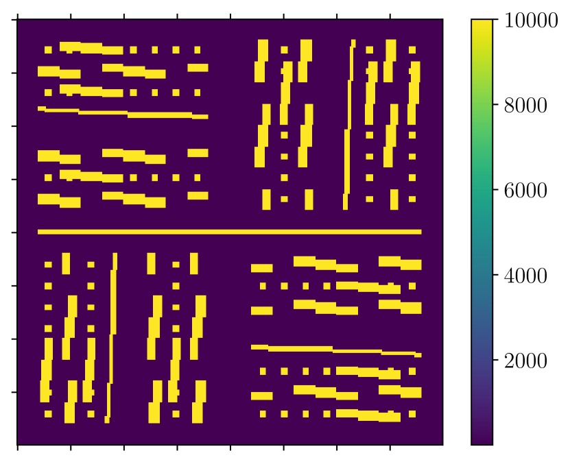
(a)

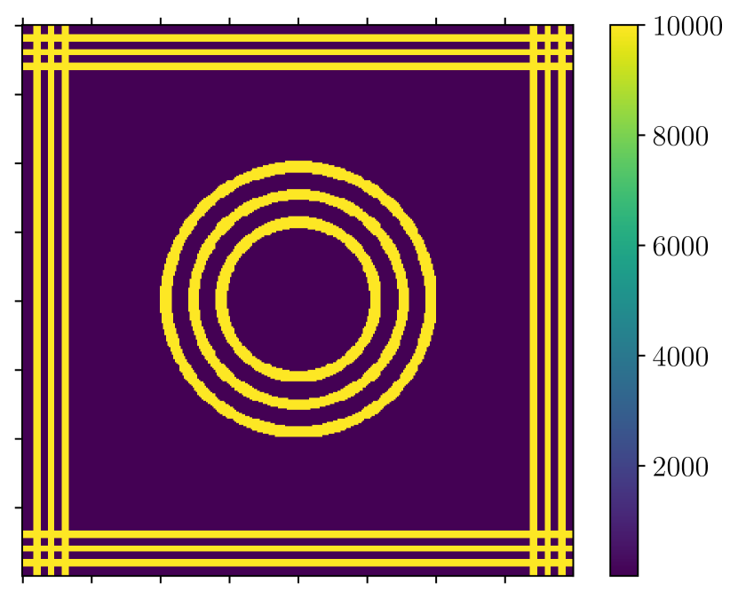
(b)

(c)

Figure 1: (a) The medium configuration cfg-a; (b) the medium configuration cfg-b; (c) the source term $f$.

4.1 Model problem 1

We consider the following model problem:

$$\left\{\begin{aligned} &-\operatorname{div}\left(\kappa(x_{1},x_{2})\nabla u\right)=f(x_{1},x_{2})\ &\forall(x_{1},x_{2})\in\Omega,\\ &u(x_{1},x_{2})=\tilde{g}(x_{1},x_{2})=x_{1}^{2}+\exp(x_{1}x_{2})\ &\forall(x_{1},x_{2})\in\partial\Omega,\end{aligned}\right.$$ (23)

where $\kappa$ is generated from cfg-a with various $\kappa_{\textnormal{I}}$ and the source term $f$ is a piecewise constant function whose value are taken via fig. 1.

We first examine the exponential convergence of $\left(\mathcal{D}^{m}-\mathcal{D}^{\textnormal{glo}}\right)\tilde{g}$ by setting $H=1/20$ and $l_{\textnormal{m}}=2$. The results are reported in table 1, where we introduce notations

$$\textnormal{D}_{a}^{m}\coloneqq\frac{\left\lVert\left(\mathcal{D}^{m}-\mathcal{D}^{\textnormal{glo}}\right)\tilde{g}\right\rVert_{a}}{\left\lVert\mathcal{D}^{\textnormal{glo}}\tilde{g}\right\rVert_{a}}\quad\text{and}\quad\textnormal{D}_{L}^{m}\coloneqq\frac{\left\lVert\left(\mathcal{D}^{m}-\mathcal{D}^{\textnormal{glo}}\right)\tilde{g}\right\rVert_{L^{2}(\Omega)}}{\left\lVert\mathcal{D}^{\textnormal{glo}}\tilde{g}\right\rVert_{L^{2}(\Omega)}}$$

to measure errors, and $\Lambda^{\prime}=\max_{i}\lambda_{i}^{l_{\textnormal{m}}}$ as a reference for $\Lambda$. We can see that the fluctuation of $\Lambda^{\prime}$ with respect to the contrast ratio $\kappa_{\textnormal{I}}/\kappa_{\textnormal{m}}$ is almost unnoticeable in our test cases, which partly explains the effectiveness of the CEM-GMsFEM in high contrast problems. This observation is quite interest, and we can transform it into a formal mathematical conjecture: is it possible to bound $\lambda$ which is an eigenvalue of

$$\int_{\Omega}\kappa\nabla u\cdot\nabla v\,\mathrm{d}x=\lambda\int_{\Omega}\kappa uv\,\mathrm{d}x\quad\forall v\in H^{1}(\Omega)$$

with $C\textnormal{diam}\left(\Omega\right)^{d}$ while the constant $C$ is independent with $\sup_{x}\kappa/\inf_{x}\kappa$? As predicted in corollary 1, the convergence behavior of $\textnormal{D}_{a}^{m}$ should solely depend on $\Lambda$, and our numerical results strongly support this argument. Comparing $\left\lVert\mathcal{D}^{\textnormal{glo}}\right\rVert_{a}$ with $\left\lVert\mathcal{D}^{\textnormal{glo}}\right\rVert_{L^{2}(\Omega)}$, we can find $\left\lVert\mathcal{D}^{\textnormal{glo}}\right\rVert_{a}$ is almost linearly dependent on contrast ratios while such a relation is not significant on $\left\lVert\mathcal{D}^{\textnormal{glo}}\right\rVert_{L^{2}(\Omega)}$. However, the exponential convergence property can allow us to compensate errors from $\left\lVert\mathcal{D}^{\textnormal{glo}}\right\rVert_{a}$ through a modest larger oversampling region.

Table 1: All the numerical tests are performed under $H=1/20$ and $l_{\textnormal{m}}=2$. The results include relative errors between $\mathcal{D}^{\textnormal{glo}}\tilde{g}$ and $\mathcal{D}^{m}\tilde{g}$ with respect to different oversampling layers $m$ and contrast ratios $\kappa_{\textnormal{I}}/\kappa_{\textnormal{m}}$, and the values of $\Lambda^{\prime}=\max_{i}\lambda_{i}^{l_{\textnormal{m}}}$, $\left\lVert\mathcal{D}^{\textnormal{glo}}\tilde{g}\right\rVert_{a}$ and $\left\lVert\mathcal{D}^{\textnormal{glo}}\tilde{g}\right\rVert_{L^{2}(\Omega)}$ with different contrast ratios.

$\kappa_{\textnormal{I}}/\kappa_{\textnormal{m}}$	$1.000\text{\times}{10}^{4}$	$1.000\text{\times}{10}^{5}$	$1.000\text{\times}{10}^{6}$
$\Lambda^{\prime}$	$1.149\text{\times}{10}^{00}$	$1.149\text{\times}{10}^{00}$	$1.149\text{\times}{10}^{00}$
$\textnormal{D}_{a}^{1}$	$1.052\text{\times}{10}^{-2}$	$1.051\text{\times}{10}^{-2}$	$1.051\text{\times}{10}^{-02}$
$\textnormal{D}_{a}^{2}$	$2.575\text{\times}{10}^{-4}$	$2.568\text{\times}{10}^{-4}$	$2.567\text{\times}{10}^{-04}$
$\textnormal{D}_{a}^{3}$	$6.679\text{\times}{10}^{-6}$	$6.592\text{\times}{10}^{-6}$	$6.583\text{\times}{10}^{-06}$
$\textnormal{D}_{a}^{4}$	$<$$1.000\text{\times}{10}^{-6}$	$<$$1.000\text{\times}{10}^{-6}$	$<$$1.000\text{\times}{10}^{-6}$
$\left\lVert\mathcal{D}^{\textnormal{glo}}\right\rVert_{a}$	$6.767\text{\times}{10}^{01}$	$2.140\text{\times}{10}^{02}$	$6.769\text{\times}{10}^{02}$
$\textnormal{D}_{L}^{1}$	$3.944\text{\times}{10}^{-02}$	$3.941\text{\times}{10}^{-02}$	$3.941\text{\times}{10}^{-02}$
$\textnormal{D}_{L}^{2}$	$1.583\text{\times}{10}^{-03}$	$1.582\text{\times}{10}^{-03}$	$1.582\text{\times}{10}^{-03}$
$\textnormal{D}_{L}^{3}$	$1.440\text{\times}{10}^{-04}$	$1.438\text{\times}{10}^{-04}$	$1.438\text{\times}{10}^{-04}$
$\textnormal{D}_{L}^{4}$	$<$$1.000\text{\times}{10}^{-6}$	$<$$1.000\text{\times}{10}^{-6}$	$<$$1.000\text{\times}{10}^{-6}$
$\left\lVert\mathcal{D}^{\textnormal{glo}}\right\rVert_{L^{2}(\Omega)}$	$6.947\text{\times}{10}^{-03}$	$6.952\text{\times}{10}^{-03}$	$6.953\text{\times}{10}^{-03}$

In the second experiment, we fix $\kappa_{\textnormal{I}}/\kappa_{\textnormal{m}}=10^{4}$ and $l_{\text{m}}=2$ to display how numerical solution errors, i.e.,

$$\textnormal{E}_{a}^{m}\coloneqq\frac{\left\lVert w^{m}-\mathcal{D}^{m}\tilde{g}-u_{0}\right\rVert_{a}}{\left\lVert u\right\rVert_{a}}\quad\text{and}\quad\textnormal{E}_{a}^{m}\coloneqq\frac{\left\lVert w^{m}-\mathcal{D}^{m}\tilde{g}-u_{0}\right\rVert_{L^{2}(\Omega)}}{\left\lVert u\right\rVert_{L^{2}(\Omega)}}$$

change with coarse mesh sizes $H$ and oversampling layers $m$. The results are reported in table 2. An important observation is that errors will increase if we only reduce $H$ while not enlarge oversampling layers $m$, which is distinct from traditional finite element methods. Actually, if focusing on $m=1$, we can see that $\textnormal{E}_{a}^{1}$ grows like $O(H^{-1})$. Recalling the error expression in theorem 2, such a numerical evidence supports the estimate $\left\lVert\pi w^{\textnormal{glo}}\right\rVert_{s}=O(H^{-1})$. Due to the competence between $\left\lVert\pi w^{\textnormal{glo}}\right\rVert_{s}$ and $m$, the minimal error occurs in the setting ($H=1/40,m=4$) rather than ($H=1/80,m=4$). Another interesting point is that, when $m=1$, errors in the $L^{2}$ norm ($\approx 8\%$) are greatly smaller than ones in the energy norm ($70\%\sim 600\%$). Since $L^{2}$ norms can not reflect small oscillations of functions, we may image that by gradually increasing oversampling layers, numerical solutions obtained by the CEM-GMsFEM capture “macroscale” information first then resolve “finescale” details.

Table 2: The numerical errors of the model problem eq. 23 in the energy and $L^{2}$ norm with different coarse mesh sizes $H$ and oversampling layers $m$, while contrast ratios and eigenvector numbers are fixed as $\kappa_{\textnormal{I}}/\kappa_{\textnormal{m}}=10^{4}$ and $l_{\textnormal{m}}=2$.

$H$	$1/10$	$1/20$	$1/40$	$1/80$
$\textnormal{E}_{a}^{1}$	$7.702\text{\times}{10}^{-01}$	$1.453\text{\times}{10}^{00}$	$3.065\text{\times}{10}^{00}$	$6.029\text{\times}{10}^{00}$
$\textnormal{E}_{a}^{2}$	$4.023\text{\times}{10}^{-02}$	$8.161\text{\times}{10}^{-02}$	$2.005\text{\times}{10}^{-01}$	$4.401\text{\times}{10}^{-01}$
$\textnormal{E}_{a}^{3}$	$2.662\text{\times}{10}^{-03}$	$2.632\text{\times}{10}^{-03}$	$7.753\text{\times}{10}^{-03}$	$2.301\text{\times}{10}^{-02}$
$\textnormal{E}_{a}^{4}$	$2.308\text{\times}{10}^{-03}$	$4.283\text{\times}{10}^{-04}$	$3.041\text{\times}{10}^{-04}$	$1.035\text{\times}{10}^{-03}$
$\textnormal{E}_{L}^{1}$	$6.957\text{\times}{10}^{-02}$	$6.603\text{\times}{10}^{-02}$	$7.445\text{\times}{10}^{-02}$	$8.062\text{\times}{10}^{-02}$
$\textnormal{E}_{L}^{2}$	$6.789\text{\times}{10}^{-04}$	$3.237\text{\times}{10}^{-03}$	$1.664\text{\times}{10}^{-02}$	$4.581\text{\times}{10}^{-02}$
$\textnormal{E}_{L}^{3}$	$7.070\text{\times}{10}^{-05}$	$7.016\text{\times}{10}^{-06}$	$2.860\text{\times}{10}^{-05}$	$2.315\text{\times}{10}^{-04}$
$\textnormal{E}_{L}^{4}$	$6.638\text{\times}{10}^{-05}$	$4.857\text{\times}{10}^{-06}$	$1.079\text{\times}{10}^{-06}$	$1.079\text{\times}{10}^{-06}$

In the third experiment, we focus on numerical errors with different contrast ratios and oversampling layers, and record the results in table 3, where we set $H=1/80$ and $l_{\textnormal{m}}=2$. It is not surprise that high contrast ratios will deteriorate numerical accuracy. However, the exponential convergence in $m$ alleviates this deterioration. Actually, the numerical accuracy of ($\kappa_{\textnormal{I}}/\kappa_{\textnormal{m}}=10^{6},m=4$) improves almost $20$ times comparing to ($\kappa_{\textnormal{I}}/\kappa_{\textnormal{m}}=10^{6},m=3$). Similarly, as emphasized in the second experiment, the $L^{2}$ norm errors ($\approx 8\%$) are significantly smaller than energy norm errors ($190\%\sim 600\%$) when $m=1$. This phenomenon reveals the potential of the CEM-GMsFEM in discovering homogenized surrogate models of high contrast problems Chung et al. (2018b).

Table 3: The numerical errors the model problem eq. 23 in the energy and $L^{2}$ norm with different contrast rations $\kappa_{\textnormal{I}}/\kappa_{\textnormal{m}}$ and oversampling layers $m$, while coarse mesh sizes and eigenvector numbers are fixed as $H=1/80$ and $l_{\textnormal{m}}=2$.

$\kappa_{\textnormal{I}}/\kappa_{\textnormal{m}}$	$1.000\text{\times}{10}^{3}$	$1.000\text{\times}{10}^{4}$	$1.000\text{\times}{10}^{5}$	$1.000\text{\times}{10}^{6}$
$\textnormal{E}_{a}^{1}$	$1.944\text{\times}{10}^{00}$	$6.029\text{\times}{10}^{00}$	$1.902\text{\times}{10}^{01}$	$6.013\text{\times}{10}^{01}$
$\textnormal{E}_{a}^{2}$	$1.790\text{\times}{10}^{-01}$	$4.401\text{\times}{10}^{-01}$	$1.061\text{\times}{10}^{00}$	$3.002\text{\times}{10}^{00}$
$\textnormal{E}_{a}^{3}$	$7.882\text{\times}{10}^{-03}$	$2.301\text{\times}{10}^{-02}$	$7.097\text{\times}{10}^{-02}$	$2.075\text{\times}{10}^{-01}$
$\textnormal{E}_{a}^{4}$	$3.943\text{\times}{10}^{-04}$	$1.035\text{\times}{10}^{-03}$	$3.141\text{\times}{10}^{-03}$	$9.882\text{\times}{10}^{-03}$
$\left\lVert u\right\rVert_{a}$	$2.826\text{\times}{10}^{00}$	$2.841\text{\times}{10}^{00}$	$2.843\text{\times}{10}^{00}$	$2.843\text{\times}{10}^{00}$
$\textnormal{E}_{L}^{1}$	$7.866\text{\times}{10}^{-02}$	$8.062\text{\times}{10}^{-02}$	$8.086\text{\times}{10}^{-02}$	$8.089\text{\times}{10}^{-02}$
$\textnormal{E}_{L}^{2}$	$1.330\text{\times}{10}^{-02}$	$4.581\text{\times}{10}^{-02}$	$6.632\text{\times}{10}^{-02}$	$7.250\text{\times}{10}^{-02}$
$\textnormal{E}_{L}^{3}$	$2.968\text{\times}{10}^{-05}$	$2.315\text{\times}{10}^{-04}$	$2.174\text{\times}{10}^{-03}$	$1.657\text{\times}{10}^{-02}$
$\textnormal{E}_{L}^{4}$	$1.079\text{\times}{10}^{-06}$	$1.079\text{\times}{10}^{-06}$	$9.175\text{\times}{10}^{-06}$	$1.241\text{\times}{10}^{-05}$
$\left\lVert u\right\rVert_{L^{2}(\Omega)}$	$1.853\text{\times}{10}^{00}$	$1.853\text{\times}{10}^{00}$	$1.853\text{\times}{10}^{00}$	$1.853\text{\times}{10}^{00}$

We test numerical errors with different $l_{m}$ in the fourth experiment, and the other parameters are set as ($H=1/80,\kappa_{\textnormal{I}}/\kappa_{\textnormal{m}}=10^{6},m=3$). It is natural that providing more eigenvectors in constructing $V^{\textnormal{aux}}$ performance will be better. However, the numerical report table 4 shows that error may not be reduced proportionally to eigenvector numbers. Because adding more eigenvectors improves convergence rates through increasing $\Lambda$, which we only know the asymptotic behavior when $l_{\textnormal{m}}\rightarrow\infty$ (i.e., Weyl’s law Ivrii (2016)). In practice, $3$ or $4$ eigenvectors is enough for obtaining satisfying accuracy, and there are several rules of thumb in determining how many eigenvectors should be applied when high conductivity channels appear Chung et al. (2018a).

Table 4: The numerical errors the model problem eq. 23 in the energy and $L^{2}$ norm with different numbers ($l_{\textnormal{m}}+1$) of eigenvectors applied in constructing $V^{\textnormal{aux}}_{i}$, while other parameters are fixed as ($H=1/80,\kappa_{\textnormal{I}}/\kappa_{\textnormal{m}}=10^{6},m=3$).

$l_{\textnormal{m}}$	$0$	$1$	$2$	$3$
$\textnormal{E}_{a}^{3}$	$8.002\text{\times}{10}^{-01}$	$4.932\text{\times}{10}^{-01}$	$2.301\text{\times}{10}^{-02}$	$2.109\text{\times}{10}^{-02}$
$\textnormal{E}_{L}^{3}$	$6.297\text{\times}{10}^{-02}$	$3.589\text{\times}{10}^{-02}$	$2.315\text{\times}{10}^{-04}$	$2.002\text{\times}{10}^{-04}$

4.2 Model problem 2

In this subsection, we study the following inhomogeneous Neumann BVP:

$$\left\{\begin{aligned} &-\operatorname{div}\left(\kappa(x_{1},x_{2})\nabla u\right)=f(x_{1},x_{2})\ &\forall(x_{1},x_{2})\in\Omega,\\ &u(x_{1},x_{2})=0\ &\forall(x_{1},x_{2})\in(0,1)\times\{1\},\\ &\nu\cdot\kappa\nabla u=q(x_{1},x_{2})=-1\ &\forall(x_{1},x_{2})\in\{0\}\times(0,1),\\ &\nu\cdot\kappa\nabla u=q(x_{1},x_{2})=1\ &\forall(x_{1},x_{2})\in\{1\}\times(0,1),\\ &\nu\cdot\kappa\nabla u=q(x_{1},x_{2})=1\ &\forall(x_{1},x_{2})\in(0,0.5)\times\{0\},\\ &\nu\cdot\kappa\nabla u=q(x_{1},x_{2})=0\ &\forall(x_{1},x_{2})\in(0.5,1)\times\{0\},\\ \end{aligned}\right.$$ (24)

where $\kappa$ is generated from cfg-b with various $\kappa_{\textnormal{I}}$ and the source term $f$ is a piecewise constant function whose value are taken via fig. 1.

We first plot $\mathcal{N}^{\textnormal{glo}}q$ under different contrast ratios ($\kappa_{\textnormal{I}}/\kappa_{\textnormal{m}}=1,10,10^{2},10^{3}$) in fig. 2, and note that when $\kappa_{\textnormal{I}}/\kappa_{\textnormal{m}}=1$ the medium is homogeneous. Due to high conductivity channels contacting with boundary, we can see from fig. 2 that on the four corners of $\Omega$, $\mathcal{N}^{\textnormal{glo}}q$ of the test case ($\kappa_{\textnormal{I}}/\kappa_{\textnormal{m}}=1$) on ${\Gamma_{\textnormal{N}}}$ is different from rest cases. Moreover, all figures show that $\mathcal{N}^{\textnormal{glo}}q$ decays rapidly away from boundaries, which is already predicted by corollary 1. We also collect several numerical results table 5 to illustrate this point, where notations

$$\textnormal{N}_{a}^{m}\coloneqq\frac{{\left\lVert\left(\mathcal{N}^{m}-\mathcal{N}^{\textnormal{glo}}\right)q\right\rVert}_{a}}{\left\lVert\mathcal{N}^{\textnormal{glo}}q\right\rVert_{a}}\quad\text{and}\quad\textnormal{N}_{L}^{m}\coloneqq\frac{\left\lVert\left(\mathcal{N}^{m}-\mathcal{N}^{\textnormal{glo}}\right)q\right\rVert_{L^{2}(\Omega)}}{\left\lVert\mathcal{D}^{\textnormal{glo}}q\right\rVert_{L^{2}(\Omega)}}$$

are adopted. We can read from table 5 that changes of $\Lambda^{\prime}$ is quite small, which has been observed in section 4.1. Owing to this fact, even we multiply by $10$ on contrast ratios column by column, convergence histories of $\textnormal{N}_{a}^{m}$ along with $m$ are still similar. The major difference with table 1 is that $\left\lVert\mathcal{N}^{\textnormal{glo}}\right\rVert_{a}$ does not grow linearly with respect to contrast ratios. This can be explained by the estimate $\left\lVert\mathcal{N}^{\textnormal{glo}}\right\rVert_{a}\leq C_{\textnormal{tr}}\left\lVert q\right\rVert_{L^{2}({\Gamma_{\textnormal{N}}})}$, and we may postulate that the influence of contrast ratios on $C_{\textnormal{tr}}$ is limited.

(a)

(b)

(c)

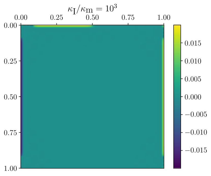
(d)

Figure 2: Plot $\mathcal{N}^{\textnormal{glo}}q$ with different contrast ratios. Note that (a) is distinct from (b) to (d) on the four corners of the domain.

Table 5: All the numerical tests are performed under $H=1/20$ and $l_{\textnormal{m}}=2$. The results include relative errors between $\mathcal{N}^{\textnormal{glo}}\tilde{g}$ and $\mathcal{N}^{m}\tilde{g}$ with respect to different oversampling layers $m$ and contrast ratios $\kappa_{\textnormal{I}}/\kappa_{\textnormal{m}}$, and the values of $\Lambda^{\prime}=\max_{i}\lambda_{i}^{l_{\textnormal{m}}}$, $\left\lVert\mathcal{N}^{\textnormal{glo}}q\right\rVert_{a}$ and $\left\lVert\mathcal{N}^{\textnormal{glo}}q\right\rVert_{L^{2}(\Omega)}$ with different contrast ratios.

$\kappa_{\textnormal{I}}/\kappa_{\textnormal{m}}$	$1.0\text{\times}{10}^{2}$	$1.0\text{\times}{10}^{3}$	$1.0\text{\times}{10}^{4}$	$1.0\text{\times}{10}^{5}$	$1.0\text{\times}{10}^{6}$
$\Lambda^{\prime}$	$8.726\text{\times}{10}^{-01}$	$8.802\text{\times}{10}^{-01}$	$8.810\text{\times}{10}^{-01}$	$8.811\text{\times}{10}^{-01}$	$8.811\text{\times}{10}^{-01}$
$\textnormal{N}_{a}^{1}$	$9.941\text{\times}{10}^{-03}$	$9.949\text{\times}{10}^{-03}$	$9.949\text{\times}{10}^{-03}$	$9.949\text{\times}{10}^{-03}$	$9.949\text{\times}{10}^{-03}$
$\textnormal{N}_{a}^{2}$	$3.133\text{\times}{10}^{-04}$	$1.911\text{\times}{10}^{-04}$	$1.760\text{\times}{10}^{-04}$	$1.709\text{\times}{10}^{-04}$	$1.709\text{\times}{10}^{-04}$
$\left\lVert\mathcal{N}^{\textnormal{glo}}q\right\rVert_{a}$	$1.979\text{\times}{10}^{-01}$	$1.988\text{\times}{10}^{-01}$	$1.989\text{\times}{10}^{-01}$	$1.989\text{\times}{10}^{-01}$	$1.989\text{\times}{10}^{-01}$
$\textnormal{N}_{L}^{1}$	$8.127\text{\times}{10}^{-03}$	$8.475\text{\times}{10}^{-03}$	$8.467\text{\times}{10}^{-03}$	$8.467\text{\times}{10}^{-03}$	$8.467\text{\times}{10}^{-03}$
$\textnormal{N}_{L}^{2}$	$<$$1.000\text{\times}{10}^{-6}$	$<$$1.000\text{\times}{10}^{-6}$	$<$$1.000\text{\times}{10}^{-6}$	$<$$1.000\text{\times}{10}^{-6}$	$<$$1.000\text{\times}{10}^{-6}$
$\left\lVert\mathcal{N}^{\textnormal{glo}}q\right\rVert_{L^{2}(\Omega)}$	$2.338\text{\times}{10}^{-03}$	$2.360\text{\times}{10}^{-03}$	$2.362\text{\times}{10}^{-03}$	$2.362\text{\times}{10}^{-03}$	$2.362\text{\times}{10}^{-03}$

The next experiment is parallel to the third experiment in section 4.1, and the main objective is verifying the effectiveness of the method proposed in high contrast settings. We choose $H=1/80$ and $l_{\textnormal{m}}=2$, and the results are listed in table 6, where a similar convergence pattern as table 3 can be observed. We again emphasized that to achieve expected numerical accuracy, enlarging oversampling regions is necessary.

Table 6: The numerical errors of the model problem eq. 24 in the energy and $L^{2}$ norm with different contrast rations $\kappa_{\textnormal{I}}/\kappa_{\textnormal{m}}$ and oversampling layers $m$, while coarse mesh sizes and eigenvector numbers are fixed as $H=1/80$ and $l_{\textnormal{m}}=2$.

$\kappa_{\textnormal{I}}/\kappa_{\textnormal{m}}$	$1.000\text{\times}{10}^{3}$	$1.000\text{\times}{10}^{4}$	$1.000\text{\times}{10}^{5}$	$1.000\text{\times}{10}^{6}$
$\textnormal{E}_{a}^{1}$	$5.847\text{\times}{10}^{-01}$	$4.263\text{\times}{10}^{-01}$	$3.956\text{\times}{10}^{-01}$	$3.922\text{\times}{10}^{-01}$
$\textnormal{E}_{a}^{2}$	$2.535\text{\times}{10}^{-01}$	$3.499\text{\times}{10}^{-01}$	$3.784\text{\times}{10}^{-01}$	$3.820\text{\times}{10}^{-01}$
$\textnormal{E}_{a}^{3}$	$1.290\text{\times}{10}^{-02}$	$3.155\text{\times}{10}^{-02}$	$9.060\text{\times}{10}^{-02}$	$2.321\text{\times}{10}^{-01}$
$\textnormal{E}_{a}^{4}$	$7.495\text{\times}{10}^{-04}$	$1.415\text{\times}{10}^{-03}$	$3.644\text{\times}{10}^{-03}$	$1.117\text{\times}{10}^{-02}$
$\left\lVert u\right\rVert_{a}$	$2.508\text{\times}{10}^{-01}$	$2.206\text{\times}{10}^{-01}$	$2.168\text{\times}{10}^{-01}$	$2.164\text{\times}{10}^{-01}$
$\textnormal{E}_{L}^{1}$	$9.582\text{\times}{10}^{-01}$	$9.575\text{\times}{10}^{-01}$	$9.578\text{\times}{10}^{-01}$	$9.578\text{\times}{10}^{-01}$
$\textnormal{E}_{L}^{2}$	$3.579\text{\times}{10}^{-01}$	$7.894\text{\times}{10}^{-01}$	$9.280\text{\times}{10}^{-01}$	$9.461\text{\times}{10}^{-01}$
$\textnormal{E}_{L}^{3}$	$9.784\text{\times}{10}^{-04}$	$6.477\text{\times}{10}^{-03}$	$5.321\text{\times}{10}^{-02}$	$3.491\text{\times}{10}^{-01}$
$\textnormal{E}_{L}^{4}$	$<$$1.000\text{\times}{10}^{-6}$	$<$$1.000\text{\times}{10}^{-6}$	$6.489\text{\times}{10}^{-05}$	$7.804\text{\times}{10}^{-04}$
$\left\lVert u\right\rVert_{L^{2}(\Omega)}$	$1.942\text{\times}{10}^{-02}$	$1.575\text{\times}{10}^{-02}$	$1.541\text{\times}{10}^{-02}$	$1.538\text{\times}{10}^{-02}$

4.3 Model problem 3

In this subsection, we consider the following inhomogeneous Robin BVP:

$$\left\{\begin{aligned} &-\operatorname{div}\left(\kappa(x_{1},x_{2})\nabla u\right)=f(x_{1},x_{2})\ &\forall(x_{1},x_{2})\in\Omega,\\ &\nu\cdot\kappa(x_{1},x_{2})\nabla u+\mathbf{b}(x_{1},x_{2})u=q(x_{1},x_{2})\ &\forall(x_{1},x_{2})\in\partial\Omega,\end{aligned}\right.$$ (25)

where $\kappa(x_{1},x_{2})$ is generated from cfg-b with $\mathbf{b}(x_{1},x_{2})=\kappa(x_{1},x_{2})$, and $q(x_{1},x_{2})$ is defined as

$$q(x_{1},x_{2})=\left\{\begin{aligned} &-1\quad\text{on}\quad\{0\}\times(0,1),\\ &1\quad\text{on}\quad\{1\}\times(0,1),\\ &1\quad\text{on}\quad(0,0.5)\times\{0\},\quad 0\quad\text{on}\quad(0.5,1)\times\{0\},\\ &0\quad\text{on}\quad(0,0.5)\times\{1\},\quad-1\quad\text{on}\quad(0.5,1)\times\{1\}.\end{aligned}\right.$$

Note that $\mathbf{b}(x_{1},x_{2})$ is also high contrast now, and traditional methods need a very fine mesh to resolve the channel structure and special treatments to solve final linear systems. The numerical results of our method are listed in table 7, which shows that the reliability of our method even with a $10^{6}$ contrast ratio.

Table 7: The numerical errors of the model problem eq. 25 in the energy and $L^{2}$ norm with different contrast rations $\kappa_{\textnormal{I}}/\kappa_{\textnormal{m}}$ and oversampling layers $m$, while coarse mesh sizes and eigenvector numbers are fixed as $H=1/80$ and $l_{\textnormal{m}}=2$.

$\kappa_{\textnormal{I}}/\kappa_{\textnormal{m}}$	$1.000\text{\times}{10}^{3}$	$1.000\text{\times}{10}^{4}$	$1.000\text{\times}{10}^{5}$	$1.000\text{\times}{10}^{6}$
$\textnormal{E}_{a}^{1}$	$5.293\text{\times}{10}^{-01}$	$3.960\text{\times}{10}^{-01}$	$3.711\text{\times}{10}^{-01}$	$3.684\text{\times}{10}^{-01}$
$\textnormal{E}_{a}^{2}$	$2.135\text{\times}{10}^{-01}$	$3.248\text{\times}{10}^{-01}$	$3.544\text{\times}{10}^{-01}$	$3.581\text{\times}{10}^{-01}$
$\textnormal{E}_{a}^{3}$	$1.091\text{\times}{10}^{-02}$	$2.933\text{\times}{10}^{-02}$	$8.487\text{\times}{10}^{-02}$	$2.175\text{\times}{10}^{-01}$
$\textnormal{E}_{a}^{4}$	$6.657\text{\times}{10}^{-04}$	$1.315\text{\times}{10}^{-03}$	$3.414\text{\times}{10}^{-03}$	$1.046\text{\times}{10}^{-02}$
$\left\lVert u\right\rVert_{a}$	$2.584\text{\times}{10}^{-01}$	$2.342\text{\times}{10}^{-01}$	$2.311\text{\times}{10}^{-01}$	$2.308\text{\times}{10}^{-01}$
$\textnormal{E}_{L}^{1}$	$9.494\text{\times}{10}^{-01}$	$9.555\text{\times}{10}^{-01}$	$9.565\text{\times}{10}^{-01}$	$9.565\text{\times}{10}^{-01}$
$\textnormal{E}_{L}^{2}$	$3.613\text{\times}{10}^{-01}$	$7.899\text{\times}{10}^{-01}$	$9.269\text{\times}{10}^{-01}$	$9.449\text{\times}{10}^{-01}$
$\textnormal{E}_{L}^{3}$	$1.008\text{\times}{10}^{-03}$	$6.499\text{\times}{10}^{-03}$	$5.315\text{\times}{10}^{-02}$	$3.487\text{\times}{10}^{-01}$
$\textnormal{E}_{L}^{4}$	$<$$1.000\text{\times}{10}^{-6}$	$<$$1.000\text{\times}{10}^{-6}$	$6.490\text{\times}{10}^{-05}$	$7.795\text{\times}{10}^{-04}$
$\left\lVert u\right\rVert_{L^{2}(\Omega)}$	$1.687\text{\times}{10}^{-02}$	$1.554\text{\times}{10}^{-02}$	$1.541\text{\times}{10}^{-02}$	$1.540\text{\times}{10}^{-02}$

References

- Bensoussan et al. [2011] A. Bensoussan, J.-L. Lions, and G. Papanicolaou. Asymptotic analysis for periodic structures. AMS Chelsea Publishing, Providence, RI, 2011. ISBN 978-0-8218-5324-5. doi:10.1090/chel/374. Corrected reprint of the 1978 original [MR0503330].
- Dal Maso [1993] Gianni Dal Maso. An introduction to -convergence, volume 8 of Progress in Nonlinear Differential Equations and their Applications. Birkhäuser Boston, Inc., Boston, MA, 1993. ISBN 0-8176-3679-X. doi:10.1007/978-1-4612-0327-8.
- Jikov et al. [1994] V. V. Jikov, S. M. Kozlov, and O. A. Oleĭnik. Homogenization of differential operators and integral functionals. Springer-Verlag, Berlin, 1994. ISBN 3-540-54809-2. doi:10.1007/978-3-642-84659-5. Translated from the Russian by G. A. Yosifian [G. A. Iosif\cprimeyan].
- Pankov [1997] Alexander Pankov. -convergence and homogenization of nonlinear partial differential operators, volume 422 of Mathematics and its Applications. Kluwer Academic Publishers, Dordrecht, 1997. ISBN 0-7923-4720-X. doi:10.1007/978-94-015-8957-4.
- Conca and Vanninathan [1997] Carlos Conca and Muthusamy Vanninathan. Homogenization of periodic structures via Bloch decomposition. SIAM Journal on Applied Mathematics, 57(6):1639–1659, 1997. ISSN 0036-1399. doi:10.1137/S0036139995294743.
- Cioranescu and Donato [1999] Doina Cioranescu and Patrizia Donato. An introduction to homogenization, volume 17 of Oxford Lecture Series in Mathematics and its Applications. The Clarendon Press, Oxford University Press, New York, 1999. ISBN 0-19-856554-2.
- Cioranescu et al. [2008] D. Cioranescu, A. Damlamian, and G. Griso. The periodic unfolding method in homogenization. SIAM Journal on Mathematical Analysis, 40(4):1585–1620, 2008. ISSN 0036-1410. doi:10.1137/080713148.
- Tartar [2009] Luc Tartar. The general theory of homogenization, volume 7 of Lecture Notes of the Unione Matematica Italiana. Springer-Verlag, Berlin; UMI, Bologna, 2009. ISBN 978-3-642-05194-4. doi:10.1007/978-3-642-05195-1. A personalized introduction.
- Shen [2018] Zhongwei Shen. Periodic homogenization of elliptic systems, volume 269 of Operator Theory: Advances and Applications. Birkhäuser/Springer, Cham, 2018. ISBN 978-3-319-91213-4; 978-3-319-91214-1. doi:10.1007/978-3-319-91214-1. Advances in Partial Differential Equations (Basel).
- Armstrong et al. [2019] Scott Armstrong, Tuomo Kuusi, and Jean-Christophe Mourrat. Quantitative stochastic homogenization and large-scale regularity, volume 352 of Grundlehren der Mathematischen Wissenschaften [Fundamental Principles of Mathematical Sciences]. Springer, Cham, 2019. ISBN 978-3-030-15544-5; 978-3-030-15545-2; 978-3-030-15547-6. doi:10.1007/978-3-030-15545-2.
- Hou and Wu [1997] Thomas Y. Hou and Xiao-Hui Wu. A multiscale finite element method for elliptic problems in composite materials and porous media. Journal of Computational Physics, 134(1):169–189, 1997. ISSN 0021-9991. doi:10.1006/jcph.1997.5682.
- Hou et al. [1999] Thomas Y. Hou, Xiao-Hui Wu, and Zhiqiang Cai. Convergence of a multiscale finite element method for elliptic problems with rapidly oscillating coefficients. Mathematics of Computation, 68(227):913–943, 1999. ISSN 0025-5718. doi:10.1090/S0025-5718-99-01077-7.
- Chen and Hou [2003] Zhiming Chen and Thomas Y. Hou. A mixed multiscale finite element method for elliptic problems with oscillating coefficients. Mathematics of Computation, 72(242):541–576, 2003. ISSN 0025-5718. doi:10.1090/S0025-5718-02-01441-2.
- Efendiev and Hou [2009] Yalchin Efendiev and Thomas Y. Hou. Multiscale finite element methods, volume 4 of Surveys and Tutorials in the Applied Mathematical Sciences. Springer, New York, 2009. ISBN 978-0-387-09495-3. Theory and applications.
- E and Engquist [2003] Weinan E and Bjorn Engquist. The heterogeneous multiscale methods. Communications in Mathematical Sciences, 1(1):87–132, 2003. ISSN 1539-6746.
- E et al. [2005] Weinan E, Pingbing Ming, and Pingwen Zhang. Analysis of the heterogeneous multiscale method for elliptic homogenization problems. Journal of the American Mathematical Society, 18(1):121–156, 2005. ISSN 0894-0347. doi:10.1090/S0894-0347-04-00469-2.
- Abdulle et al. [2012] Assyr Abdulle, Weinan E, Björn Engquist, and Eric Vanden-Eijnden. The heterogeneous multiscale method. Acta Numerica, 21:1–87, 2012. ISSN 0962-4929. doi:10.1017/S0962492912000025.
- Hughes [1995] Thomas J. R. Hughes. Multiscale phenomena: Green’s functions, the Dirichlet-to-Neumann formulation, subgrid scale models, bubbles and the origins of stabilized methods. Computer Methods in Applied Mechanics and Engineering, 127(1-4):387–401, 1995. ISSN 0045-7825. doi:10.1016/0045-7825(95)00844-9.
- Brezzi et al. [1997] F. Brezzi, L. P. Franca, T. J. R. Hughes, and A. Russo. . Computer Methods in Applied Mechanics and Engineering, 145(3-4):329–339, 1997. ISSN 0045-7825. doi:10.1016/S0045-7825(96)01221-2.
- Hughes and Sangalli [2007] T. J. R. Hughes and G. Sangalli. Variational multiscale analysis: the fine-scale Green’s function, projection, optimization, localization, and stabilized methods. SIAM Journal on Numerical Analysis, 45(2):539–557, 2007. ISSN 0036-1429. doi:10.1137/050645646.
- Babuska and Lipton [2011] Ivo Babuska and Robert Lipton. Optimal local approximation spaces for generalized finite element methods with application to multiscale problems. Multiscale Modeling & Simulation. A SIAM Interdisciplinary Journal, 9(1):373–406, 2011. ISSN 1540-3459. doi:10.1137/100791051.
- Babuška et al. [2020] Ivo Babuška, Robert Lipton, Paul Sinz, and Michael Stuebner. Multiscale-spectral GFEM and optimal oversampling. Computer Methods in Applied Mechanics and Engineering, 364:112960, 28, 2020. ISSN 0045-7825. doi:10.1016/j.cma.2020.112960.
- Efendiev et al. [2013] Yalchin Efendiev, Juan Galvis, and Thomas Y. Hou. Generalized multiscale finite element methods (GMsFEM). Journal of Computational Physics, 251:116–135, 2013. ISSN 0021-9991. doi:10.1016/j.jcp.2013.04.045.
- Chung et al. [2014] Eric T. Chung, Yalchin Efendiev, and Wing Tat Leung. Generalized multiscale finite element methods for wave propagation in heterogeneous media. Multiscale Modeling & Simulation. A SIAM Interdisciplinary Journal, 12(4):1691–1721, 2014. ISSN 1540-3459. doi:10.1137/130926675.
- Chung et al. [2016] Eric Chung, Yalchin Efendiev, and Thomas Y. Hou. Adaptive multiscale model reduction with generalized multiscale finite element methods. Journal of Computational Physics, 320:69–95, 2016. ISSN 0021-9991. doi:10.1016/j.jcp.2016.04.054.
- Må lqvist and Peterseim [2014] Axel Må lqvist and Daniel Peterseim. Localization of elliptic multiscale problems. Mathematics of Computation, 83(290):2583–2603, 2014. ISSN 0025-5718. doi:10.1090/S0025-5718-2014-02868-8.
- Henning and Må lqvist [2014] Patrick Henning and Axel Må lqvist. Localized orthogonal decomposition techniques for boundary value problems. SIAM Journal on Scientific Computing, 36(4):A1609–A1634, 2014. ISSN 1064-8275. doi:10.1137/130933198.
- Altmann et al. [2021] Robert Altmann, Patrick Henning, and Daniel Peterseim. Numerical homogenization beyond scale separation. Acta Numerica, 30:1–86, 2021. ISSN 0962-4929. doi:10.1017/S0962492921000015.
- Hellman and Må lqvist [2017] Fredrik Hellman and Axel Må lqvist. Contrast independent localization of multiscale problems. Multiscale Modeling & Simulation. A SIAM Interdisciplinary Journal, 15(4):1325–1355, 2017. ISSN 1540-3459. doi:10.1137/16M1100460.
- Må lqvist and Peterseim [2021] A. Må lqvist and D. Peterseim. Numerical homogenization by localized orthogonal decomposition, volume 5 of SIAM Spotlights. Society for Industrial and Applied Mathematics (SIAM), Philadelphia, PA, 2021. ISBN 978-1-611976-44-1.
- Chung et al. [2018a] Eric T. Chung, Yalchin Efendiev, and Wing Tat Leung. Constraint energy minimizing generalized multiscale finite element method. Computer Methods in Applied Mechanics and Engineering, 339:298–319, 2018a. ISSN 0045-7825. doi:10.1016/j.cma.2018.04.010.
- Vasilyeva et al. [2019] Maria Vasilyeva, Eric T. Chung, Yalchin Efendiev, and Jihoon Kim. Constrained energy minimization based upscaling for coupled flow and mechanics. Journal of Computational Physics, 376:660–674, 2019. ISSN 0021-9991. doi:10.1016/j.jcp.2018.09.054.
- Wang et al. [2021] Yiran Wang, Eric Chung, and Lina Zhao. Constraint energy minimization generalized multiscale finite element method in mixed formulation for parabolic equations. Mathematics and Computers in Simulation, 188:455–475, 2021.
- Chung and Pun [2020] Eric Chung and Sai-Mang Pun. Computational multiscale methods for first-order wave equation using mixed CEM-GMsFEM. Journal of Computational Physics, 409:109359, 13, 2020. ISSN 0021-9991. doi:10.1016/j.jcp.2020.109359.
- Bellieud and Bouchitté [1998] Michel Bellieud and Guy Bouchitté. Homogenization of elliptic problems in a fiber reinforced structure. Nonlocal effects. Annali della Scuola Normale Superiore di Pisa. Classe di Scienze. Serie IV, 26(3):407–436, 1998. ISSN 0391-173X.
- Briane [2002] Marc Briane. Homogenization of non-uniformly bounded operators: critical barrier for nonlocal effects. Archive for Rational Mechanics and Analysis, 164(1):73–101, 2002. ISSN 0003-9527. doi:10.1007/s002050200196.
- Du et al. [2020] Qiang Du, Bjorn Engquist, and Xiaochuan Tian. Multiscale modeling, homogenization and nonlocal effects: mathematical and computational issues. In 75 years of mathematics of computation, volume 754 of Contemp. Math., pages 115–139. Amer. Math. Soc., [Providence], RI, 2020. doi:10.1090/conm/754/15175.
- Scott and Zhang [1990] L. Ridgway Scott and Shangyou Zhang. Finite element interpolation of nonsmooth functions satisfying boundary conditions. Mathematics of Computation, 54(190):483–493, 1990. ISSN 0025-5718. doi:10.2307/2008497.
- Brenner and Scott [2008] Susanne C. Brenner and L. Ridgway Scott. The mathematical theory of finite element methods, volume 15 of Texts in Applied Mathematics. Springer, New York, third edition, 2008. ISBN 978-0-387-75933-3. doi:10.1007/978-0-387-75934-0.
- Brezzi and Fortin [1991] Franco Brezzi and Michel Fortin. Mixed and hybrid finite element methods, volume 15 of Springer Series in Computational Mathematics. Springer-Verlag, New York, 1991. ISBN 0-387-97582-9. doi:10.1007/978-1-4612-3172-1.
- Harris et al. [2020] Charles R. Harris, K. Jarrod Millman, Stéfan J. van der Walt, Ralf Gommers, Pauli Virtanen, David Cournapeau, Eric Wieser, Julian Taylor, Sebastian Berg, Nathaniel J. Smith, Robert Kern, Matti Picus, Stephan Hoyer, Marten H. van Kerkwijk, Matthew Brett, Allan Haldane, Jaime Fernández del Río, Mark Wiebe, Pearu Peterson, Pierre Gérard-Marchant, Kevin Sheppard, Tyler Reddy, Warren Weckesser, Hameer Abbasi, Christoph Gohlke, and Travis E. Oliphant. Array programming with NumPy. Nature, 585(7825):357–362, September 2020. doi:10.1038/s41586-020-2649-2.
- Virtanen et al. [2020] Pauli Virtanen, Ralf Gommers, Travis E. Oliphant, Matt Haberland, Tyler Reddy, David Cournapeau, Evgeni Burovski, Pearu Peterson, Warren Weckesser, Jonathan Bright, Stéfan J. van der Walt, Matthew Brett, Joshua Wilson, K. Jarrod Millman, Nikolay Mayorov, Andrew R. J. Nelson, Eric Jones, Robert Kern, Eric Larson, C J Carey, İlhan Polat, Yu Feng, Eric W. Moore, Jake VanderPlas, Denis Laxalde, Josef Perktold, Robert Cimrman, Ian Henriksen, E. A. Quintero, Charles R. Harris, Anne M. Archibald, Antônio H. Ribeiro, Fabian Pedregosa, Paul van Mulbregt, and SciPy 1.0 Contributors. SciPy 1.0: Fundamental Algorithms for Scientific Computing in Python. Nature Methods, 17:261–272, 2020. doi:10.1038/s41592-019-0686-2.
- Chung et al. [2018b] Eric T. Chung, Yalchin Efendiev, Wing Tat Leung, Maria Vasilyeva, and Yating Wang. Non-local multi-continua upscaling for flows in heterogeneous fractured media. Journal of Computational Physics, 372:22–34, 2018b. ISSN 0021-9991. doi:10.1016/j.jcp.2018.05.038.
- Ivrii [2016] Victor Ivrii. 100 years of Weyl’s law. Bulletin of Mathematical Sciences, 6(3):379–452, 2016. ISSN 1664-3607. doi:10.1007/s13373-016-0089-y.