A Geometric Approach to $k$-means

Abstract

$k$-means clustering is a fundamental problem in various disciplines. This problem is nonconvex, and standard algorithms are only guaranteed to find a local optimum. Leveraging the structure of local solutions characterized in [1], we propose a general algorithmic framework for escaping undesirable local solutions and recovering the global solution (or the ground truth). This framework consists of alternating between the following two steps iteratively: (i) detect mis-specified clusters in a local solution and (ii) improve the current local solution by non-local operations. We discuss implementation of these steps, and elucidate how the proposed framework unifies variants of $k$-means algorithm in literature from a geometric perspective. In addition, we introduce two natural extensions of the proposed framework, where the initial number of clusters is misspecified. We provide theoretical justification for our approach, which is corroborated with extensive experiments.

1 Introduction

Clustering is fundamental problem across machine learning, computer vision, statistics and beyond. The general goal of clustering is to group a large number of high dimensional data points into a few clusters of similar points. Many clustering criteria have been proposed. Specifically, the $k$-means formulation aims to find $k$ cluster centers such that the sum of squared distance between data points to the nearest cluster center is minimized. The most popular algorithm for $k$-means is Lloyd’s algorithm [2] which iteratively updates the cluster assignment for each data point and the location of cluster centers. The $k$-means problem is nonconvex, and hence Lloyd’s and other local search algorithms (typically with random initialization) are only guaranteed to find a local solution in general.

With decades of extensive research and application, various improved algorithms have been proposed for $k$-means to address the sub-optimality of local solutions. One line of algorithms focus on careful initialization. The celebrated $k$-means++ initialization [3] employs a probabilistic initialization scheme such that the initial cluster centers are spread out. For a comprehensive review of initialization methods, see [4]. Another line of work aims at fine tuning a local solution to produce a better solution based on various heuristics and empirical observations of the local solutions [5, 6, 7, 8, 9, 10, 11]. However, in absence of a precise characterization of the local solutions, little can be guaranteed about the performance of these heuristics.

On the theory side, recent years have witnessed exciting progress on demystifying the structure of local solutions in certain nonconvex problems [12, 13, 14, 15, 16, 17, 18, 19], including $k$-means and related clustering problems. It is known that when the data are sampled from two identical spherical Gaussians, the Expectation-Maximization (EM) algorithm recovers ground truth solution from a random initialization [20, 21, 22]. Similar results hold for Lloyd’s algorithm when the two Gaussians satisfy certain separation conditions [23]. However, as soon as the number of Gaussian components exceeds three, additional local solutions emerge, whose quality can be arbitrarily worse than the global optimum [24]. Recent work has established an interesting positive result showing that under some separation conditions, all the local solutions share the same geometric structure that provides partial information for the ground-truth, under both the $k$-means [1] and the negative log-likelihood [25] formulations.

In this paper, we exploit the algorithmic implications of the above structural results for the geometry for the $k$-means local solutions. We propose a general algorithmic framework for recovering the global minimizer (or ground truth clusters) from a local minimizer. Our framework consists of iterating two steps: (i) detect mis-specified clusters in a local solution obtained by Lloyd’s algorithm, and (ii) improve the current local solution by non-local operations. This geometry-inspired framework is non-probabilistic and does not rely on a good initialization. Under certain mixture models with $k$ clusters, we prove that the proposed framework requires $O(k)$ iterations to recover the ground truth, whereas standard Lloyd’s algorithm would require $e^{\Omega(k)}$ random initializations to achieve the same. The framework is flexible and provides justifications for many existing heuristics. Our approach can be naturally extended to settings when the initial number of clusters is misspecified. Extensive experiments demonstrate that our approaches perform robustly on challenging benchmark datasets.

2 Structure of Local Solutions

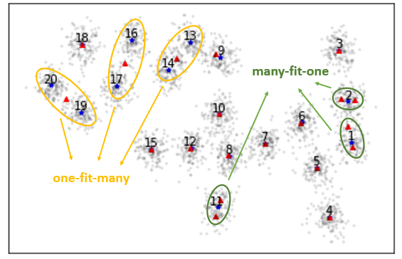
Figure 1: one-fit-many and many-fit-one association in a local minima of the $k$-means problem.

We consider the $k$-means problem under a mixture model with $k^{*}$ components: each data point $\bm{x}$ is sampled i.i.d. from a true density $f^{*}:=\frac{1}{k^{*}}\sum_{s=1}^{k^{*}}f^{*}_{s}$, where $f^{*}_{s}$ is the density of the $s$-th component with mean $\bm{\beta}_{s}^{*}\in^{d}$. Under this generative model, the population $k$-means objective function is

$$G(\bm{\beta}):=\mathbb{E}_{\bm{x}\sim f^{*}}\min_{j\in[k]}\|\bm{x}-\bm{\beta}_{j}\|^{2},\vspace{-.1in}$$ (1)

where $\bm{\beta}=(\bm{\beta}_{1},\ldots,\bm{\beta}_{k})$ denotes $k$ fitted cluster centers, with $k$ potentially different from $k^{*}$. The objective function $G$ is non-convex, and standard algorithms like Lloyd’s only guarantee finding a local minimizer. Nevertheless, a recent work [1] shows that all local minima have the same geometric structure. In particular, [1] establishes that under some separation condition, for every local minimum solution $\bm{\beta}$, there exists an association map $\mathcal{A}$ between a partition of the fitted centers $\{\bm{\beta}_{s}\}_{s\in[k]}$ and a partition of the true centers $\{\bm{\beta}^{\star}_{s}\}_{s\in[k^{*}]}$, such that each center must involve exactly one of three types of association:

1. one-fit-many association: a fitted center $\bm{\beta}_{i}$ encompasses several true clusters with centers $\left\{\bm{\beta}^{\star}_{j}\right\}_{j\in S}$, for some $S\subseteq[k^{*}]$. Equivalently, $\mathcal{A}(\left\{\bm{\beta}_{i}\right\})=\{\bm{\beta}^{\star}_{j}\}_{j\in S}$.

2. many-fit-one association: several fitted centers $\{\bm{\beta}_{i}\}_{i\in T}$ split a true cluster with center $\bm{\beta}^{\star}_{j}$, for some $T\subseteq[k]$ and $j\in[k^{*}]$. Equivalently, $\mathcal{A}(\{\bm{\beta}_{i}\}_{i\in T})=\{\bm{\beta}^{\star}_{j}\}$.

3. almost empty association: a fitted centers not associated with any true cluster, and the corresponding fitted cluster has almost zero measure.

Figure 1 illustrates these associations between the fitted centers (represented by red triangles) in a local minimizer and the ground truth clusters (represented by blue dots).

With the above characterization, we can infer some geometric properties of a local minimizer within each type of association, particularly when the true clusters are separated and have identical shapes. For simple exposition, we start with the Stochastic Ball Model (Section 2.1 of [1]), in which $f_{s}^{*}$ satisfies

$$f_{s}^{*}(\bm{x})=\frac{1}{\textup{Vol}(\mathbb{B}_{s}(r))}1_{\mathbb{B}_{s}(r)}(\bm{x}),\quad s\in[k^{*}],$$ (2)

where $\mathbb{B}_{s}$ denotes a ball with radius $r$ centered at $\bm{\beta}_{s}$.

One-fit-many association

A fitted center with a one-fit-many association is approximately in the center of multiple balls, thus the mean in-cluster $\ell_{2}$ distance to that fitted center is lowered bounded by the minimum separation of the balls. On the other hand, for a fitted center with a many-fit-one association, the associated fitted cluster is contained in a ball, thus the mean in-cluster $\ell_{2}$ distance to that fitted center is upper bounded by the radius of the ball. When the balls are well-separated from each other, we infer that the mean in-cluster $\ell_{2}$ distance is higher for the fitted cluster with one-fit-many association.

Many-fit-one association

Since the fitted center with a many-fit-one association is contained in a ball, the pairwise distance between two such fitted centers, that are associated with the same ball, is lower bounded by the radius of the ball. On the other hand, the distance between that fitted center and any other fitted center, that is not associated with the ball, is lower bounded by the separation of the balls. We thus infer that the fitted centers with the same association to a ball has smaller pairwise distance.

Almost empty association

A cluster with an almost empty association has a negligible measure by Theorem 1 and 2 in  [1]. This means this cluster usually contains a very small number of data points. For example, in an extreme case, some $\bm{\beta}_{j}$ can be far away from all the data points and has an empty association with the data. We usually consider a non-degenerate local minimum solution, in which no almost empty associations can occur.

The above elementary properties of the fitted clusters with one-fit-many and many-fit-one associations are derived from the ball models. In general, they may depend on the assumptions of the underlying data. As the properties for one-fit-many and many-fit-one associations are distinct, they can be leveraged to identify the exact type of association. Afterwards, various methods can be designed to eliminate these associations. Since these associations are the only hurdles to recovering a global solution, eliminating associations potentially helps escaping a local minimum solution of the $k$-means.

3 From Structure to Algorithms

Motivated by geometric structure, more precisely, the one-fit-many and many-fit-one associations, in the local minimum solutions described in Section 2, we propose a general algorithmic framework for avoiding local minimum solutions via detecting and correcting those undesirable associations. Indeed, one-fit-many association is more troublesome as none of the associated true clusters are identified in a solution. On the other hand, for the many-fit-one association, the center of each fitted clusters that are associated with the same true cluster is actually close to that true center; thus that true cluster is partially identified.

The framework is based on (1) detecting one-fit-many and many-fit-one associations in the current solution, and (2) splitting a cluster with a one-fit-many association while merging clusters with many-fit-one association. This general framework, which we call Fission-Fusion $k$-means, is described in details in Section 3.1. In Section 3.2, we discuss a few methods to detect one-fit-many and many-fit-one associations. Viewing one-fit-many and many-fit-one association as local model misspecification, we derive a natural extension of the framework in Section 3.3, which allows us to start with any number of fitted clusters. At last, we discuss other related algorithmic approaches in literature and their relationships to the framework in Section 3.4.

3.1 Fission-Fusion $k$-means

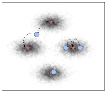
Figure 2: Fission Fusion $k$-means Illustration

The proposed framework (Algorithm 1) aims to iteratively improve the $k$-means solution. At each iteration, it first detects a fitted cluster with tentative one-fit-many association; secondly it replaces the fitted center with two centers from the 2-means solution (Fission); thirdly, it detects a pair of fitted clusters with tentative many-fit-one association and then merges these two fitted centers into one center (Fusion); finally, a Lloyd’s $k$-means step is used to update the modified solution. The above procedure is iterated until the $k$-means objective no longer decreases.

Algorithm 1 Fission-Fusion $k$-means (FFkm)

Input: data $\mathcal{D}$, number of fitted clusters $k$, initial non-degenerate solution $\bm{\beta}^{(\frac{1}{2})}\in{{}^{d\times k}}$ and the max number of iterations $L$.
      Output: $\bm{\beta}^{(L)}$

1:Using $\bm{\beta}^{(\frac{1}{2})}$ as an initial solution, run Lloyd’s algorithm to obtain a local minimum $\bm{\beta}^{(1)}$ with $k$-means objective value $G^{(1)}$. Set $G^{(0)}=\infty$ and $\ell=1$.

2:while $\ell\leq L$ do

3:     Step 1: Detect a cluster with tentative one-fit-many association, whose center is $\beta_{(1)}^{(\ell)}$.

4:     Step 2: Compute $\bm{\beta}^{(\ell+\frac{1}{2})}$ from $\bm{\beta}^{(\ell)}$ using the following procedure:

5:     - Step 2a: Split the center $\beta_{(1)}^{(\ell)}$ into two centers;

6:     - Step 2b: Detect two clusters with tentative many-fit-one association with the same true cluster, whose centers are $\beta_{(2)}^{(\ell)}$ and $\beta_{(3)}^{(\ell)}$. Merge $\beta_{(2)}^{(\ell)}$ and $\beta_{(3)}^{(\ell)}$ into one center.

7:     Step 3: Using $\bm{\beta}^{(\ell+\frac{1}{2})}$ as an initial solution, run Lloyd’s algorithm to obtain a local minimum $\bm{\beta}^{(\ell+1)}$ with $k$-means objective value $G^{(\ell+1)}$.

8:     If $G^{(\ell+1)}\geq G^{(\ell)}$, set $\bm{\beta}^{(L)}:=\bm{\beta}^{(\ell)}$, terminate.

9:     $\ell\leftarrow\ell+1$

10:end while

The algorithm maintains an invariance of the total number of fitted number of clusters in each iteration: in Step 2a, the total number of fitted clusters is increased to $k+1$; in Step 2b, the total number of fitted clusters is decreased to $k$. Moreover, Step 3 guarantees that the output solution has a $k$-means objective value no worse than the input solution. The Fission Fusion $k$-means is a general framework, as long as the one-fit-many association in Step 1 and many-fit-one association in Step 2b can be correctly identified. We note that the processes to detect one-fit-many association in Step 1 and many-fit-one association in Step 2b are flexible, and may be dependent on the data. Several methods are discussed in Section 3.2, in which the geometric properties of a local solution are harnessed.

We illustrate the working mechanism of Fission Fusion $k$-means under the stochastic ball model. For any current local minimum solution, there are two possibilities: either it is already a global optimal solution or it is a local minimum with suboptimal objective value. In the first case, the algorithm simply returns a solution whose objective value is as good as the global optimal. In the second case, the input local solution must contain a one-fit-many association following Theorem 1 of [1], as we fit $k$ clusters to $k$ true clusters. The Fission step (Step 2a) ensures that in $\bm{\beta}^{(\ell+1)}$, two (splitted) centers fit multiple (at least two) true clusters, which are contained in the cluster with one-fit-many association detected in Step 1. In particular, restricting to these true clusters, the $k$-means objective function at $\bm{\beta}^{(\ell+1)}$ strictly decreases. On the other hand, the Fusion step (Step 2b) reduces the number of centers to fit that single true cluster with which at least two fitted clusters are associated in $\bm{\beta}^{(\ell)}$. Restricting to this true cluster, the $k$-means objective function at $\bm{\beta}^{(\ell+1)}$ increases compared with that evaluated at $\bm{\beta}^{(\ell)}$. One crucial observation here is that the decrement of the $k$-means objective value from the Fission step exceeds the increase of that from the Fusion step, by at least a constant. Therefore, the Fission Fusion $k$-means must terminate at global optimal solution in a finite number of steps. The above argument can be made formal in Theorem 3.1.

Theorem 3.1 (Main Theorem)

Let $\left\{\bm{\beta}^{\star}_{i}\right\}_{i\in[k^{*}]}$ be $k^{*}$ unknown centers in ^d, with maximum and minimum separations

$$\Delta_{\max}:=\max_{i,j\in[k^{*}]}\left\|\bm{\beta}^{\star}_{i}-\bm{\beta}^{\star}_{j}\right\|,$$

$$\Delta_{\min}:=\min_{i\neq j\in[k^{*}]}\left\|\bm{\beta}^{\star}_{i}-\bm{\beta}^{\star}_{j}\right\|.$$

Suppose that the data $\bm{x}_{1},\ldots,\bm{x}_{n}\in^{d}$ is generated independently from a ball mixture model (2). Assume that $\frac{\Delta_{\min}}{r}\geq 30$. With probability at least $1-2k^{*}\exp\left(-\frac{n}{2k^{*2}}\right)$, Algorithm 1 with $k=k^{*}$ terminates in $O\left(k^{*}\cdot\frac{\Delta_{\max}^{2}}{\Delta_{\min}^{2}}\right)$ iterations and outputs a global minimizer $\bm{\beta}^{\star}$.

Under the above setting, Algorithm 1 can recover the ground truth clusters with a linear (in $k^{*}$) number of executions of the Lloyd’s algorithm . In contrast, running the Lloyd’s algorithm alone from random initialization would require an exponential number of runs to find the ground truth, shown in Theorem 3.2 below.

Theorem 3.2 (Lloyd’s Converges to Bad Locals)

In the ball mixture setting as above, let $\bm{\beta}^{(t)}$ be the $t$-th iterate in the Lloyd’s algorithm starting from a random initialization that is uniformly sampled from data. There exists a universal constant $c$, for any $k\geq 3$ and any constant $C_{\textup{gap}}>0$, such that there is a well-separated stochastic ball model with $k$ true centers with

$$\mathbb{P}\left[\forall t\geq 0:\frac{G(\bm{\beta}^{(t)})-G(\bm{\beta}^{\star})}{G(\bm{\beta}^{\star})}\geq C_{\textup{gap}}\right]\geq 1-e^{-ck},\vspace{-.1in}$$

where $G$ is the $k$-means objective defined in Eq.(1).

We defer proof of above theorems to Appendix A and B.

3.2 Detection Subroutines

We propose a few subroutines to detect one-fit-many association and many-fit-one association that utilizes the inferred properties of the local solutions described in Section 2.

Detect one-fit-many: Standard Deviation (SD)

For each $i$-th fitted cluster with center $\bm{\beta}_{i}$, we compute the mean squared $\ell_{2}$ distance to its center:

$$\sigma_{i}^{2}:=\frac{1}{|C_{i}|}\sum_{j:\bm{x}_{j}\in C_{i}}\|\bm{x}_{j}-\bm{\beta}_{i}\|^{2},$$ (3)

$$C_{i}=\big{\{}\bm{x}_{j}\in\mathcal{D}:\|\bm{x}_{j}-\bm{\beta}_{i}\|\leq\|\bm{x}_{j}-\bm{\beta}_{i^{\prime}}\|\;\forall\;i^{\prime}\neq i\big{\}}.\vspace{-.2in}$$

The subroutine outputs $i^{*}$-th cluster that attains the maximal mean squared distance:

$$i^{*}:=\text{argmax}_{i\in[k]}\sigma_{i}^{2}.\vspace{-.05in}$$ (4)

As discussed in Section 2, when the true clusters are identical in size (the stochastic ball model), a fitted cluster with a one-fit-many association contains multiple true clusters, thus having a larger mean squared distance. When the true clusters have varying size, we can adapt the above process accordingly. For example, before computing the mean squared distance for each cluster, we can normalize each cluster such that the radius (the maximal distance between a data in the cluster to the cluster center) of each fitted cluster is the same. For a fitted cluster with a one-fit-many association, the mass of the data points will concentrate near the boundary after normalization, and will have a larger mean squared distance.

Detect one-fit-many: $\epsilon$-Radius

Fix an $\epsilon>0$. For each fitted cluster $i$, we compute the percentage of points contained in $\mathbb{B}_{\epsilon}(\bm{\beta}_{i})$, which is a ball centered at $\bm{\beta}_{i}$ with radius $\epsilon$, among all the data contained in $i$-th fitted cluster:

$$p_{i}:=\frac{|B_{i}|}{|C_{i}|},\quad B_{i}=\left\{\bm{x}_{j}:\|\bm{x}_{j}-\bm{\beta}_{i}\|\leq\epsilon,\;\bm{x}_{j}\in C_{i}\right\}.\vspace{-.1in}$$

The subroutine outputs the $i^{*}$-th cluster that attains the smallest $B_{i}$:

$$i^{*}:=\text{argmin}_{i\in[k]}B_{i}.\vspace{-.1in}$$ (5)

For a fitted cluster with one-fit-many association, its center $\bm{\beta}_{i}$ is in the middle of several true clusters. There are two possibilities, either there is no true cluster near the fitted center, or the fitted center coincides with a true cluster center. In the previous case, the set $B_{i}$ is almost empty as $\bm{\beta}_{i}$ is not close to any true cluster when there are sufficient separation among the true clusters. In the latter case, the set $B_{i}$ has a small cardinality. However, $|C_{i}|$ is big as it contains multiple true clusters. In both cases, the ratio will be smaller for a cluster with a one-fit-many association (compared with a cluster with a many-fit-one association).

Detect one-fit-many: Total Deviation (TD)

For each $i$-th fitted cluster with center $\bm{\beta}_{i}$, we compute the summation of $\ell_{2}$ distance to its center:

$$v_{i}^{2}:=\sum_{j:\bm{x}_{j}\in C_{i}}\|\bm{x}_{j}-\bm{\beta}_{i}\|^{2},$$ (6)

$$C_{i}=\big{\{}\bm{x}_{j}\in\mathcal{D}:\|\bm{x}_{j}-\bm{\beta}_{i}\|\leq\|\bm{x}_{j}-\bm{\beta}_{i^{\prime}}\|\;\forall\;i^{\prime}\neq i\big{\}}.\vspace{-.2in}$$

The subroutine outputs $i^{*}$-th cluster that attains the maximal mean squared distance:

$$i^{*}:=\text{argmax}_{i\in[k]}v_{i}^{2}.\vspace{-.05in}$$ (7)

Compared with the standard deviation detection method, the total deviation is an unnormalized version of standard deviation. Indeed, the total deviation approximates the improvement in the $k$-means objective value when a single fitted cluster is fitted with two centers; see section 3.1 of [11]. This coincides with the observation that the $k$-means objective function decreases more when a fitted component with one-fit-many association is split with two centers in the stochastic ball model.

Detect many-fit-one: Pairwise Distance (PD)

For each pair of fitted cluster $(i,j)$, $i\neq j$, we compute the pairwise $\ell_{2}$ distance between fitted cluster center $\bm{\beta}_{i}$ and $\bm{\beta}_{j}$: $d_{i,j}:=\|\bm{\beta}_{i}-\bm{\beta}_{j}\|.$ The subroutine outputs $i_{*}$-th and $j_{*}$-th clusters whose pairwise distance attains the minimal:

$$(i_{*},j_{*}):=\text{argmin}_{(i,j),i\neq j}d_{i,j}.$$ (8)

The method is also based on the inferred geometric properties in Section 2: when true clusters have similar shape or size, the pairwise distance between the fitted clusters with many-fit-one association is smaller.

Detect many-fit-one: Objective Increment (OI)

For each $i$-th fitted center, let us consider a modified $k$-means clustering solution $\widehat{\bm{\beta}}^{(i)}$:

$$\widehat{\bm{\beta}}^{(i)}=(\bm{\beta}_{1},\ldots,\widehat{\bm{\beta}_{i}},\ldots,\bm{\beta}_{k})$$

by removing the $i$-th center. Denote the corresponding $k$-means objective function as $G_{i}$, in which we fit $k-1$ centers to the data compared with the original clustering solution. Let $(i^{*},j^{*})$ be such that

$$i^{*}= \text{argmin}_{i}G_{i},$$

$$j^{*}= \text{argmin}_{j,j\neq i^{*}}\|\bm{\beta}_{j}-\bm{\beta}_{i}^{*}\|.$$

This method coincides with the observation that the $k$-means objective function increases the least when two fitted centers that have many-fit-one association with the same true center are merged in the stochastic ball model.

Detection Procedure from Literature

The idea of using split and merge in clustering problem can be traced back as early as 1960s [27]. It has been used to determine the correct number of fitted clusters when $k$ is unknown [5, 6, 8], or to escape local solution when $k$ is known [28, 7]. Several criteria for split and merge step have been proposed in literature; see Table 1. These criteria can be adapted to our proposed framework, and we describe below in details.

In $X$-means [5, 6], the Bayesian Information Criterion (BIC) score with respect to the corresponding solution is computed. A fitted cluster is to be split into two clusters if the BIC score decreases and a pair of clusters are to be merged if the BIC score decreases. To adapt the split criteria to detecting one-fit-many association in our framework, we can output the cluster that attains the maximal reduction in BIC score if it is split into two cluster; to adapt the merge criteria to detecting many-fit-one association, we can output the pair of clusters that attain the maximal reduction in BIC if they are to be merged.

The work [8] evaluates the intra-cluster and inter-cluster dissimilarity. A fitted cluster is to be split if the intra-cluster dissimilarity exceeds some threshold, and a pair of clusters are to be merged if the inter-cluster dissimilarity do not exceed some threshold. All these dissimilarity are based on Euclidean distance. To adapt the split criteria to detecting one-fit-many association, we can output the cluster with maximal intra-cluster dissimilarity; on the other hand, we can output the pair of clusters with minimal inter-cluster dissimilarity as many-fit-one association.

The work [7] attempts to split a cluster into $2,\ldots,M$ clusters and compute the ratio of successive $k$-means objective. The cluster will be split if the minimum of these ratios is smaller than a threshold. In the merge step, it retains the splittd cluster that is furthest from the neighboring regions and then merges the rest of split clusters to the neighboring voronoi regions. We can also adapt the split criteria to detecting one-fit-many association here — we can split a cluster into $2$ clusters and compute the ratio between the local $k$-means objective with 2 clusters and the local $k$-means objective with only 1 cluster. Afterwards, we output the cluster that attains the smallest ratio.

Table 1: Related Split and Merge criteria, details in Appendix C

Algorithm	Split Criteria	Merge Criteria
$X$-means [5, 6]	Reduction in BIC score	Reduction in BIC score
[8]	Max and Min in-cluster distance	Pairwise center distance
[7]	Ratio of objective value with different $k$	Pairwise center distance

3.3 Initial Parameter Misspecification

As the structural result from [1] holds for arbitrary $k$, we can utilize this observation in the algorithm. An interpretation of one-fit-many association is that an insufficient number of parameters (in this case only one parameter) are used to fit multiple true components, resulting in locally underfitting. On the other hand, many-fit-one association happens when more parameters are used to fit a single components, resulting in local overfitting. When the fitted parameter $k$ is much smaller than the ground truth $k^{*}$, the local solutions is more likely to contain one-fit-many association; conversely, when the fitted parameter $k$ is larger than the ground truth $k^{*}$, the local solutions is more likely to contain many-fit-one association. Based on this insight, there are two natural extensions of the Fission Fusion $k$-means framework starting with $k$ not necessarily equal to $k^{*}$.

(Mild-)Overparametrization

We first fit more clusters than the true number of clusters. Afterwards, we can apply many-fit-one detection subroutines and then merge close clusters. This is exactly the Fission Fusion $k$-means without the Fission step.

Algorithm 2 Overparamatrized $k$-means

Input: data $\mathcal{D}$, number of fitted clusters $k$, the number of true clusters $k^{*}$
      Output: $\bm{\beta}$

1:Run Lloyd’s algorithm initialized from $k$ randomly selected cluster centers.

2:while $k>k^{*}$ do

3:     Step 1: Detect two clusters with many-fit-one association, whose centers are $\bm{\beta}_{(1)}$ and $\bm{\beta}_{(2)}$.

4:     Step 2: Merge $\bm{\beta}_{(1)}$ and $\bm{\beta}_{(2)}$ into one center $\bm{\beta}_{(1,2)}$ by averaging, $k\leftarrow k-1$.

5:     Step 3: Run Lloyd’s algorithm on $k$ cluster centers initialized at the updated solution.

6:end while

Underparametrization

We first fit less clusters than the true number of clusters. Afterwards, we can apply one-fit-many detection subroutines and then split the clusters. This is exactly the Fission Fusion $k$-means without the Fusion step.

Algorithm 3 Underparamatrized $k$-means

Input: data points $\bm{x}_{1},...,\bm{x}_{n}\in^{d}$, number of fitted clusters $k$, number of true clusters $k^{*}$
      Output: $\bm{\beta}$

1:Run Lloyd’s algorithm initialized from $k$ randomly selected cluster centers.

2:while $k>k^{*}$ do

3:     Step 1: Detect a cluster with one-fit-many association, whose center is $\bm{\beta}_{(1)}$.

4:     Step 2: Split $\bm{\beta}_{(1)}$ into two centers $\bm{\beta}_{(1)}$ and $\bm{\beta}_{(1)^{\prime}}$ , $k\leftarrow k+1$

5:     Step 3: Run Lloyd’s algorithm on $k$ cluster centers initialized at the updated solution.

6:end while

3.4 Related Works

The proposed Fission Fusion $k$-means is a general framework to reduce one-fit-many and many-fit-one associations in each iteration, and decreases the $k$-means objective successively. It allows us to unify past algorithmic designs for $k$-means from the perspective of the structural properties of local solutions. In this section, we discuss other variants of $k$-means algorithms in literature and their connection to the proposed framework as well as to the structural properties of the local solution.

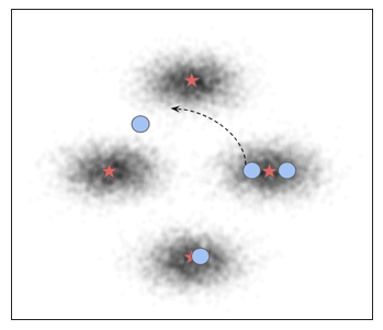
Figure 3: Swap $k$-means

One variant of the proposed framework is Swap, which moves the center of one cluster in many-fit-one association to the neighborhood of the center with one-fit-many association. This can also be viewed as performing the Fusion step before the Fission step in the current framework. Using Swap, a cluster with many-fit-one association and a cluster with one-fit-many association need to be identified simultaneously. A randomized procedure is considered in [9], in which a random center and a random cluster are swapped. Other deterministic procedures are proposed [10, 11, 29, 30, 31, 11]. To select a center to be swapped, objective value based criteria is considered in [10, 11]; merge based criteria is used in [29, 30]. To select a cluster to which a center is moved, objective value based criteria is considered in [11]; other heuristic criteria are proposed, e.g., selecting a cluster with the largest variance [32, 31].

An orthogonal direction to improve the quality of the $k$-means solution is to design careful initialization. The work by Celebi et al [4] provides a comprehensive review of the initialization methods. Inspecting those methods, many of them coincide with the intuition of reducing the one-fit-many association and many-fit-one association. We list a few examples to illustrate as an exhaustive comparison is beyond the scope of the current work. One approach is to spread out the centers sequentially, which avoids the many-fit-one association: $k$ means++ [3] uses a probabilistic procedeure; maxmin method [33] and Hartigan method [34] use a deterministic procedure. Astrahan’s method [35, 36] select centers such that the data near each center has a relative high density (with respect to the data) and successive centers are far apart from each other. Here, the proposed framework can be thought of as a simple yet principled procedure to further improve the solution regardless of sophisticated initialization routines. In particular, the proposed framework can be applied to any $k$-means solution.

4 Experiments

We evaluate the Fission-Fusion $k$-means with one-fit-many and many-fit-one association detection methods proposed in Section 3.2 on the benchmark datasets [37]. Its performance is compared with Lloyd’s algorithm (with random and $k$-means++ initialization) and related algorithms [5, 6, 7, 8, 11]. Two variants of the framework, with misspecified initial cluster number, are also evaluated.

4.1 Benchmark Datasets

The benchmark datasets [37], which have been used extensively in evaluating clustering algorithms [38, 39, 40, 41], consist of synthetic data with different cluster numbers (A-sets) , degree of separation (S-sets), dimensionality (DIM032) and balancedness (Unbalance). We provide a brief description of these datasets below. For a visualization of the datasets; see Figure 4. For a summary of the characteristics of the datasets; see Table 2.

1. A-sets contain three sets, $A_{1}$, $A_{2}$, and $A_{3}$ ($A_{1}\subset A_{2}\subset A_{3}$), which correspond to $20,35$ and $50$ spherical clusters in ² respectively, all with $20\%$ overlap.

2. S-sets contain four sets, $S_{1}$, $S_{2}$, $S_{3}$ and $S_{4}$, which correspond to $15$ Gaussian clusters in ² with varying overlap from $9\%$, $22\%$, $41\%$ and $44\%$. Most clusters are spherical, and a few have been truncated to resemble non-spherical shape.

3. Unbalance contains a single set with 8 clusters in ² belonging to two well-separated groups (left and right). The group in the lefthand side consists of 3 clusters, and the group in the righthand side consists of 5 clusters. The lefthand side group consists of much more data points than the other.

4. DIM032 contains a single set with $16$ well-separated Gaussian clusters in ³².

5. Birch1 contains a single set with $100$ Gaussian clusters in ², whose centers form a regular 10x10 grid.

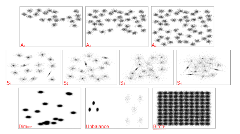
Figure 4: Visualization for the Benchmark Datasets

Table 2: Characteristics of the Benchmark Datasets.

Dataset	Varying	Size	Clusters	Per cluster
(i) A-sets	Number of clusters	3000–7500	20,35,50	150
(ii) S-sets	Overlap	5000	15	333
(iii) Dim032	Dimensions	1024x100	16	64
(iv) Birch1	Structure	100,000	100	1000
(v) Unbalance	Balance	6500	8	100–2000

4.2 Evaluation Metric

Three metrics have been used for evaluation. The first two metrics are based on a modified version of centroid index (CI) [42]. centroid index allows us to compare two clustering solutions with different number of clusters, since related algorithms such as [5, 6] do not necessarily return a solution with $k^{*}$ clusters. To compute centroid index, we first identify the index of the closest ground truth center to each fitted cluster center. Secondly, we count the total number of ground truth centers whose indices are not mapped to any fitted cluster center in the first step, and the total number gives us centroid index. Centroid index approximately measures the total number of true centers contained in one-fit-many associations. It does not penalizing many-fit-one associations, since the true center associated with that many-fit-one association has been identified. Using centroid index, we now introduce two main metrics.

• Success rate (SR): percentage of random trials an algorithm returns a clustering solution with 0 CI, i.e., all ground truth centers have been identified [37].

• Average missing rate (AMR): mean CI (normalized by true clusters number) over multiple random trials of an algorithm. Compared with success rate, it measures the solution quality of an algorithm when the success rate is not $100\%$. A higher CI indicates worse solution quality.

When an algorithm assumes the knowledge of number of true clusters ($k^{*}$), we further use the relative $k$-means objective value as a metric for comparison that is described below:

• $\rho$-ratio: the ratio between the objective value of a returned solution by an algorithm and the optimal $k$-means objective value.

4.3 Implementation and Results

We implement Algorithm 1 Fission-Fusion $k$-means (FFkm) with a combination of one-fit-many and many-fit-one detection subroutines described in Section 3.2. In particular, for one-fit-many detection, we consider standard deviation (SD), total deviation (TD) and $\epsilon$-radius (RD) methods. For many-fit-one detection, we consider the pairwise distance (PD) method and the objective increment (OI) method. There are six combinations of subroutines for implementing Fission-Fusion $k$-means in total, for which we shorthand FFkm (SD+PD), FFkm (SD+OI), FFkm (TD+PD), FFkm (TD+OI), FFkm (RD+PD), and FFkm (RD+OI) respectively.

Some additional details for implementation are described here. In the $\epsilon$-radius (RD) method, the following adaptive method has been used to determine the radius of the ball: first we compute the minimum median $\ell_{2}$ distance to cluster center among all the fitted clusters as the base radius $r$; secondly, we set the radius to be $\delta\cdot r$ ($\delta\in[0.01,0.1,1,5]$). In the subsequent experiments, we select $\delta=0.1$ as default. For the merge step (2b) in Algorithm 1, we merge two detected centroids (using either PD or OI) to their mean.

For each dataset, we execute $100$ independent trials of Algorithm 1, Lloyd’s algorithm, swap-based algorithm I-$k$-means$-$+ [11], and related algorithms [5, 7, 8]. Success Rate (SR) for each algorithm are summarized in Table 3. For those entries whose success rate is less than $100$, we also include AMR in the parenthesis to reflect the degree of missing true centers. $\rho$-ratio for algorithms with a known number of true clusters is summarized in Table 4. We include partial results (with a few combinations of subroutines) from Fission Fusion $k$-means in Table 3 and Table 4. A comprehensive results for all combinations of subroutines can be found in Table 10 in Appendix D.

We observe that the Fission Fusion $k$-means reliably recovers the ground truth solutions on almost all benchmark dataset except S3 and S4. Since the benchmark datasets vary in number of clusters, cluster shape and separation, the performance illustrates the robustness of the Fission Fusion $k$-means. S3 and S4 datasets have very high overlap among clusters, in which case the one-fit-many and many-fit-one solution structure do not necessarily hold. It is worth to note that on the benchmark dataset, the Fission Fusion $k$-means obtains comparable results as swap-based algorithm [11], as swap can be interpreted as performing a Fusion step before a Fission step. In  [11], the criteria for detecting centroids to merge and to split are based on the $k$-means objective value, similar to TD and OI detection subroutines. On the other hand, for Fission and Fusion $k$-means, the detection routines are flexible, which can be either geometry based or objective based, depending on the characteristics of the underlying dataset. As we will demonstrate in Appendix E, with geometry based detection subroutines, Fission Fusion $k$-means can produce a clustering solution with better semantic quality.

Table 3: Success rate (%) comparison (best results in boldface)

Data Set	Lloyd	$k$-means++	[11]	SD+OI	TD+OI	RD+PD	[7]	[8]	[5]
A1	1 (0.13)	49 (0.03)	100	100	100	100	99	66 (0.02)	100
A2	0 (0.13)	6 (0.04)	100	100	100	100	96	5 (0.07)	100
A3	0 (0.13)	4 (0.03)	100	100	100	100	99	0 (0.14)	0 (0.92)
S1	1 (0.14)	71 (0.02)	100	100	100	100	100	100	100
S2	3 (0.11)	61 (0.03)	100	100	100	100	90 (0.01)	100	100
S3	8 (0.09)	48 (0.04)	100	89(0.00)	96(0.00)	89(0.01)	72 (0.02)	100	100
S4	20 (0.07)	52 (0.03)	93(0.00)	39(0.04)	90(0.01)	41(0.05 )	29 (0.05)	100	98 (0.01)
Unbalance	0 (0.48)	97	100	100	100	100	17 (0.5)	99	50 (0.25)
Dim032	1 (0.21)	100	100	100	100	100	94	100	100
birch1	0 (0.07)	0	100	100	100	100	100	0 (0.08)	0 (0.96)

Table 4: $\rho$-ratio comparison (best results in boldface)

Dataset	Lloyd	$k$-means++	[11]	SD+OI	TD+OI	RD+PD	[7]
A1	$1.67\pm 0.31$	$1.12\pm 0.14$	$\bm{1.00\pm 0.00}$	$\bm{1.00\pm 0.00}$	$\bm{1.00\pm 0.00}$	$\bm{1.00\pm 0.00}$	$1.00\pm 0.02$
A2	$1.69\pm 0.24$	$1.14\pm 0.08$	$\bm{1.00\pm 0.00}$	$\bm{1.00\pm 0.00}$	$\bm{1.00\pm 0.00}$	$\bm{1.00\pm 0.00}$	$1.01\pm 0.03$
A3	$1.73\pm 0.25$	$1.13\pm 0.06$	$\bm{1.00\pm 0.00}$	$\bm{1.00\pm 0.00}$	$\bm{1.00\pm 0.00}$	$\bm{1.00\pm 0.00}$	$1.00\pm 0.01$
S1	$2.23\pm 0.55$	$1.16\pm 0.25$	$\bm{1.00\pm 0.00}$	$\bm{1.00\pm 0.00}$	$\bm{1.00\pm 0.00}$	$\bm{1.00\pm 0.00}$	$\bm{1.00\pm 0.00}$
S2	$1.56\pm 0.39$	$1.10\pm 0.13$	$\bm{1.00\pm 0.00}$	$\bm{1.00\pm 0.00}$	$\bm{1.00\pm 0.00}$	$\bm{1.00\pm 0.00}$	$1.02\pm 0.06$
S3	$1.18\pm 0.10$	$1.07\pm 0.07$	$1.01\pm 0.02$	$1.01\pm 0.04$	$\bm{1.00\pm 0.00}$	$1.01\pm 0.04$	$1.03\pm 0.06$
S4	$1.10\pm 0.08$	$1.04\pm 0.05$	$1.01\pm 0.01$	$1.05\pm 0.05$	$1.01\pm 0.02$	$1.06\pm 0.07$	$1.06\pm 0.05$
Unbalance	$9.62\pm 1.62$	$1.03\pm 0.18$	$\bm{1.00\pm 0.00}$	$\bm{1.00\pm 0.00}$	$\bm{1.00\pm 0.00}$	$\bm{1.00\pm 0.00}$	$5.14\pm 1.92$
Dim032	$51.99\pm 19.56$	$1.10\pm 1.01$	$\bm{1.00\pm 0.00}$	$\bm{1.00\pm 0.00}$	$\bm{1.00\pm 0.00}$	$\bm{1.00\pm 0.00}$	$1.70\pm 2.76$
birch1	$1.20\pm 0.04$	$1.09\pm 0.02$	$\bm{1.00\pm 0.00}$	$\bm{1.00\pm 0.00}$	$\bm{1.00\pm 0.00}$	$\bm{1.00\pm 0.00}$	$\bm{1.00\pm 0.00}$

4.4 Initial Parameter Misspecification

We execute Algorithm 2, 3 for 100 trials on the benchmark dataset. In the under-parameterized setting, we choose the initial $k$ to be $2$, $\lceil\frac{k^{*}}{4}\rceil$, and $\lceil\frac{k^{*}}{2}\rceil$. The SD method is used to detect one-fit-many association. In the over-parameterized setting, we choose the initial $k$ to be $2k^{*}$, $3k^{*}$ and $4k^{*}$. The pairwise distance is used to detect many-fit-one association. On termination of the algorithm, the number of fitted cluster is $k^{*}$, thus $\rho$-ratio is used for evaluation. A more comprehensive results of under- and over- parameterized Lloyd’s algorithm, with different initial $k$, are summarized in Table 5 and Table 6.

Table 5: Under-parameterized $k$

Dataset	$k=k^{\star}$			$k=2$			$k=\lceil\frac{k^{*}}{4}\rceil$			$k=\lceil\frac{k^{*}}{2}\rceil$
	SR(%)	AMR	$\rho$-ratio	SR(%)	AMR	$\rho$-ratio	SR(%)	AMR	$\rho$-ratio	SR(%)	AMR	$\rho$-ratio
A1	1	0.13	$1.67\pm 0.31$	100	0.00	$1.00\pm 0.00$	100	0.00	$1.00\pm 0.00$	99	0.00	$1.00\pm 0.02$
A2	0	0.13	$1.69\pm 0.24$	100	0.00	$1.00\pm 0.00$	100	0.00	$1.00\pm 0.00$	97	0.00	$1.00\pm 0.02$
A3	0	0.13	$1.73\pm 0.25$	100	0.00	$1.00\pm 0.00$	100	0.00	$1.00\pm 0.00$	92	0.00	$1.01\pm 0.02$
S1	1	0.14	$2.23\pm 0.55$	100	0.00	$1.00\pm 0.00$	100	0.00	$1.00\pm 0.00$	100	0.00	$1.00\pm 0.00$
S2	3	0.11	$1.56\pm 0.39$	100	0.00	$1.00\pm 0.00$	100	0.00	$1.00\pm 0.00$	100	0.00	$1.00\pm 0.00$
S3	8	0.09	$1.18\pm 0.10$	100	0.00	$1.00\pm 0.00$	100	0.00	$1.00\pm 0.00$	100	0.00	$1.00\pm 0.00$
S4	20	0.07	$1.10\pm 0.08$	0	0.13	$1.15\pm 0.00$	0	0.13	$1.15\pm 0.00$	0	0.07	$1.08\pm 0.02$
Unbalance	0	0.48	$9.62\pm 1.62$	100	0.00	$1.00\pm 0.00$	100	0.00	$1.00\pm 0.00$	61	0.05	$4.33\pm 4.25$
Dim032	1	0.21	$51.99\pm 19.56$	100	0.00	$1.00\pm 0.00$	99	0.00	$1.12\pm 1.17$	68	0.02	$5.25\pm 6.75$
Birch1	0	0.07	$1.20\pm 0.04$	100	0.00	$1.00\pm 0.00$	100	0.00	$1.00\pm 0.00$	100	0.00	$1.00\pm 0.00$

Table 6: Over-parameterized $k$

Dataset	$k=k^{\star}$			$k=2k^{\star}$			$k=3k^{\star}$			$k=4k^{\star}$
	SR(%)	AMR	$\rho$-ratio	SR(%)	AMR	$\rho$-ratio	SR(%)	AMR	$\rho$-ratio	SR(%)	AMR	$\rho$-ratio
A1	1	0.13	$1.67\pm 0.31$	96	0.00	$1.01\pm 0.05$	100	0.00	$1.00\pm 0.00$	100	0.00	$1.00\pm 0.00$
A2	0	0.13	$1.69\pm 0.24$	88	0.00	$1.01\pm 0.04$	99	0.00	$1.00\pm 0.01$	100	0.00	$1.00\pm 0.00$
A3	0	0.13	$1.73\pm 0.25$	89	0.00	$1.01\pm 0.03$	100	0.00	$1.00\pm 0.00$	100	0.00	$1.00\pm 0.00$
S1	1	0.14	$2.23\pm 0.55$	97	0.00	$1.02\pm 0.10$	100	0.00	$1.00\pm 0.00$	100	0.00	$1.00\pm 0.00$
S2	3	0.11	$1.56\pm 0.39$	100	0.00	$1.00\pm 0.00$	100	0.00	$1.00\pm 0.00$	100	0.00	$1.00\pm 0.00$
S3	8	0.09	$1.18\pm 0.10$	97	0.00	$1.00\pm 0.02$	100	0.00	$1.00\pm 0.00$	100	0.00	$1.00\pm 0.00$
S4	20	0.07	$1.10\pm 0.08$	85	0.01	$1.01\pm 0.03$	50	0.03	$1.04\pm 0.04$	25	0.05	$1.06\pm 0.03$
Unbalance	0	0.48	$9.62\pm 1.62$	0	0.44	$8.23\pm 2.46$	4	0.38	$6.89\pm 2.99$	6	0.34	$5.90\pm 2.93$
Dim032	1	0.21	$51.99\pm 19.56$	62	0.03	$6.88\pm 8.48$	93	0.00	$1.92\pm 3.40$	99	0.00	$1.10\pm 1.01$
Birch1	0	0.07	$1.20\pm 0.04$	100	0.00	$1.00\pm 0.00$	100	0.00	$1.00\pm 0.00$	100	0.00	$1.00\pm 0.00$

In either under-parameterized or over-parameterized setting, the returned solutions are all near optimal except for on the S4, Unbalance and DIM032 datasets. Specifically, in the under-parameterized setting, setting $k=2$ attains the best performance, while the performance is slightly worse with $k=\lceil\frac{k^{*}}{2}\rceil$. In the over-parameterized setting, setting $k=4k^{*}$ attains the best performance, and the performance is slightly worse with $k=2k^{*}$.

Discussion on Unbalance Dataset

On the Unbalance dataset, the over-parameterized setting attains poor performance. The dataset contains two groups of clusters which are far apart from each other. The first group contains 3 clusters, with smaller variance but more amount of data points; the second group contains 5 clusters, with large variance but less amount of data points. Consequently, with a random initialization, more initial centers (than the true number of contained clusters) are associated with the first group of clusters, and less initial centers are associated with the second group. Since the algorithm only performs merge step, the fitted centers can over-merge, leading to a suboptimal solution. This issue can be solved when we further increase the initial cluster number, so that we have a sufficient number of initial centers in the right part of the cluster. Indeed, the performance improves with increasing number of initial clusters; see Table 7. When $k=20k^{*}$, the over-parametrized algorithm obtains the best performance.

Table 7: Lloyd’s algorithm with over-parameterized $k$ on Unbalance dataset

k	$5k^{*}$	$6k^{*}$	$7k^{*}$	$8k^{*}$	$9k^{*}$	$10k^{*}$	$15k^{*}$	$20k^{*}$
SR	11	22	38	55	65	75	96	99
AMR	0.28	0.23	0.16	0.11	0.09	0.06	0.01	0.00
$\rho$-ratio	$4.99\pm 2.88$	$4.00\pm 2.65$	$2.97\pm 2.30$	$2.39\pm 2.08$	$2.04\pm 1.79$	$1.65\pm 1.34$	$1.11\pm 0.55$	$1.03\pm 0.30$

Table 8: $\epsilon$-Radius Detection Subroutine on S4 dataset

$\delta$	0.001	0.01	0.05	0.1	0.25	0.5	1	2	5
SR	44	41	42	41	44	40	43	39	33
AMR	0.04	0.05	0.05	0.05	0.04	0.05	0.05	0.04	0.05
$\rho$-ratio	$1.05\pm 0.07$	$1.06\pm 0.07$	$1.06\pm 0.07$	$1.06\pm 0.07$	$1.06\pm 0.07$	$1.07\pm 0.08$	$1.06\pm 0.07$	$1.05\pm 0.05$	$1.05\pm 0.04$

4.5 Real-world data

(a) Summer Palace.

(b) Boat.

(c) House.

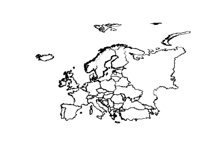
(d) Europe.

Figure 5: Real World Scenarios Data Visualization.

We consider four real world datasets: three image datasets consist of quantized RGB color values and one coordinate map of Europe maps [37], visualized in Figure 5.

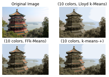
Figure 6: Visualization of Summer Palace ($k=10$)

Figure 6 and Figure 7 demonstrate the clustering results using Lloyd’s algorithm, FFkm(SD+PD) and I-$k$-means$-$+. The visual results in Figure 6 suggest that FFkm(SD+PD) and I-$k$-means$-$+ perform better than Lloyd’s algorithm; Figure 7 suggests that FFkm(SD+PD) is better than I-$k$-means$-$+ and Lloyd’s algorithm.

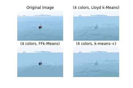
Figure 7: Visualization of Boat ($k=4$).

Table 9: Characteristics of the data sets and sum of squared errors (SSE) result.

Data Set	D	N	k	SSE of Lloyd’s	SSE of FFkm(SD+PD)	SSE of I-$k$-means$-$+
Boat	3	50325	4	$224.79\pm 4.71$	$217.70\pm 7.90$	$219.80\pm 7.33$
Palace	3	273280	64	$533.17\pm 19.04$	$514.27\pm 23.99$	$504.62\pm 23.99$
House	3	65536	256	$20.70\pm 0.48$	$19.75\pm 1.02$	$19.46\pm 0.94$
Eroupe	2	169672	256	$113101.18\pm 7671.54$	$95750.71\pm 13261.01$	$100538.85\pm 13935.38$

Table 9 summarizes the sum of squared errors (SSE) from $20$ independent execution of Lloyd’s algorithm, FFkm (SD+PD), and I-$k$-means$-$+. $D$, $N$, and $k$ denote data dimension, number, and cluster number respectively. Both FFkm and I-$k$-means$-$+ outperform the Lloyd’s algorithm.

5 Conclusion

We propose a flexible framework for $k$-means problem by harnessing the geometric structure of local solutions. It provides a theoretical foundation for future work to design detection routines for varying cluster distributions. Future work includes analyzing the Fission-Fission $k$-means under the more general setting with empirical success: (1) clusters could be of different sizes and shapes; (2) clusters have moderate or heavy overlaps with each other.

Appendix A Proof for Theorem 3.1

Proof. The $k$-means objective function is

$$G_{n}(\bm{\beta})=\frac{1}{n}\sum_{t=1}^{n}\min_{s\in[k^{*}]}\|\bm{x}_{t}-\bm{\beta}_{s}\|^{2}.$$ (9)

Note that the output solution of the algorithm is no worse than the input solution, it suffices to consider the case in which the initial solution $\bm{\beta}^{(0)}$ is a non-degenerate local minimum with a strictly worse objective value than that of a global optimal solution. Note that we fit the data with $k^{*}$ cluster, there exists a fitted cluster with one-fit-many association. Assume this is not the case, then $\bm{\beta}^{(0)}$ only has many-fit-one associations. This means that for each true cluster center, there is at least a fitted center close to it. Since $k=k^{*}$, each true cluster must be associated with exactly one fitted cluster. In particular, $\bm{\beta}^{(0)}$ is global optimal, a contradiction. Similarly, $\bm{\beta}^{(0)}$ must have two fitted clusters with many-fit-one associations.

We first characterize the amount of improvement of the $k$-means objective in each fission-and-fusion step. Specifically, Lemma A.2 shows that

$$G_{n}(\bm{\beta}^{(\frac{1}{2})})\leq G_{n}(\bm{\beta}^{(0)})-\frac{\Delta_{\min}^{2}}{72k^{*}}.$$

Since the Lloyd step (Step 3 of the algorithm) does not increase the $k$-means objective (Lemma A.3), it follows that

$$G_{n}(\bm{\beta})^{(1)})\leq G_{n}(\bm{\beta}^{(\frac{1}{2})})\leq G_{n}(\bm{\beta}^{(0)})-\frac{\Delta_{\min}^{2}}{72k^{*}}.$$

Thus after each the first iteration of the Fission-Fussion algorithm, the decrement in the $k$-means objective function is at least a constant. Moreover, $\bm{\beta}^{(1)}$ is non-degenerate local minimum from the argument in Lemma A.3. We can then apply the above argument recursively, obtaining

$$G_{n}(\bm{\beta}^{(\ell)})\leq G_{n}(\bm{\beta}^{(0)})-\ell\cdot\frac{\Delta_{\min}^{2}}{72k^{*}}.$$

Note that the $k$-means objective value is upper bounded uniformly at every non-degenerate local minimum by Lemma A.1, and lower bounded by $0$. In particular,

$$0\leq G_{n}(\bm{\beta}^{(0)})\leq 4\Delta_{\max}^{2}.$$

This means that there are at most $\frac{288k^{*}\Delta_{\max}^{2}}{\Delta_{\min}^{2}}$ Fission-Fussion iterations in the algorithm. At the termination of the algorithm, we must obtain a global optimal solution.

 

Lemma A.1 (Upper Bound)

Under the assumption of Theorem 3.1, suppose $\bm{\beta}$ is a non-degenerate local minimum of $G_{n}$. Then

$$G_{n}(\bm{\beta})\leq 4\Delta_{\max}^{2}.$$

Proof. When $\bm{\beta}$ is a non-degenerate local minimum solution, each fitted cluster is non-empty. From Lemma 2 of [1], each $\bm{\beta}_{i}$ is at the center of the corresponding Voronoi set. In particular, each $\bm{\beta}_{i}$ must be in the convex hull of all the balls. For each $i\in[k^{*}]$, we conveniently represent $\bm{\beta}_{i}$ as

$$\bm{\beta}_{i}=\sum_{s\in[k^{*}]}\alpha_{i,s}(\bm{\beta}^{\star}_{s}+\bm{v}_{i,s}),$$

where $\left\{\bm{v}_{i,s}\right\}_{s\in[k^{*}]}$ are vectors in ^d with norm bounded by $r$; $\alpha_{i,s}$s’ are non-negative scalars satisfying $\sum_{s\in[k^{*}]}\alpha_{i,s}=1$. For each $t\in[n]$, assuming without loss of generality that $\bm{x}_{t}$ is generated from $f_{1}^{*}$, we have

$$\big{\|}\bm{x}_{t}-\bm{\beta}_{i}\big{\|}= \Big{\|}\bm{\beta}^{\star}_{1}+\bm{u}-\sum_{s\in[k^{*}]}\alpha_{s}(\bm{\beta}^{\star}_{s}+\bm{v}_{s})\Big{\|}$$ (10)

$$= \Big{\|}\sum_{s\in[k^{*}]}\alpha_{s}(\bm{\beta}^{\star}_{1}-\bm{\beta}^{\star}_{s})+\sum_{s\in[k^{*}]}\alpha_{s}(\bm{u}-\bm{v}_{s})\Big{\|}$$

$$\leq \Delta_{\max}+2r\leq 2\Delta_{\max}.$$ (11)

In equation 10, we represent $\bm{x}_{t}=\bm{\beta}^{\star}_{1}+\bm{u}$ for some vector $\bm{u}\in^{d}$ with norm bounded by $r$. In inequality 11, we apply the triangle inequality and the SNR assumption that $\frac{\Delta_{\max}}{r}\geq\frac{\Delta_{\min}}{r}\geq 30$.

It follows that $G_{n}(\bm{\beta})\leq\frac{1}{n}\sum_{t\in[n]}\left(r+\Delta_{\max}\right)^{2}\leq 4\Delta_{\max}^{2}$.

 

Lemma A.2 (Improvement)

Under the assumption of Theorem 3.1, for each $\ell=0,1,2,\ldots$,

$$G_{n}(\bm{\beta}^{(\ell+\frac{1}{2})})\leq G_{n}(\bm{\beta}^{(\ell)})-\frac{\delta_{\min}^{2}}{72k^{*}}.$$

Moreover, each $\bm{\beta}^{(\ell)}$ is non-degenerate.

Proof. Using the structural result of a local minimum, if $\bm{\beta}^{(\ell)}$ is a non-degenerate local minima that is not globally optimal, then $\bm{\beta}^{(\ell)}$ must have both one-fit-many and many-fit-one association. Without loss of generality, suppose that in the local minimizer $\bm{\beta}^{(\ell)}$, the center $\bm{\beta}_{1}$ fits multiple true centers $\bm{\beta}^{\star}_{1},\ldots,\bm{\beta}^{\star}_{m}$, where $m\geq 2$, and the centers $\bm{\beta}_{2}$ and $\bm{\beta}_{3}$ (potentially along with some other centers) fit the true center $\bm{\beta}^{\star}_{m+1}$. For $i=1,\ldots,s+1$, let $C_{i}$ index the data points generated from $f_{i}^{*}$.

Suppose that in the new solution $\bm{\beta}^{(\ell+\frac{1}{2})},$ $\bm{\beta}_{1}$ is split into two centers $\bm{\beta}_{<}$ and $\bm{\beta}_{>}$, where $\bm{\beta}_{<}=\bm{\beta}_{1}$ and $\bm{\beta}_{>}$ is moved to a data point $\bm{x}_{0}=\arg\max_{\bm{x}\in\mathcal{V}(\bm{\beta}_{1})}\left\|\bm{x}-\bm{\beta}_{1}\right\|$, where $\mathcal{V}(\bm{\beta}_{1})$ is the Voronoi set associated with $\bm{\beta}_{1}$; moreover, $\bm{\beta}_{2}$ and $\bm{\beta}_{3}$ are merged into one center $\bm{\beta}_{=}=\frac{1}{2}\left(\bm{\beta}_{2}+\bm{\beta}_{3}\right)$. Suppose that $\bm{x}_{0}$ is from the cluster $C_{1}$ generated from $f_{1}^{*}$.

We illustrate the above notations in Figure 8.

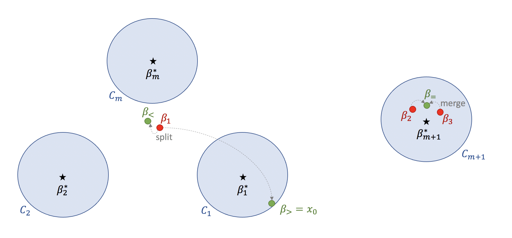
Figure 8: Illustration for Lemma A.2

The objective values before and after Fission and Fusion are

$$G_{n}(\bm{\beta}^{(\ell)}) =\frac{1}{n}\left(\sum_{i\in[m]}\sum_{t\in C_{i}}\left\|\bm{x}_{t}-\bm{\beta}_{1}\right\|^{2}+\sum_{t\in C_{m+1}}\min\left\{\left\|\bm{x}_{t}-\bm{\beta}_{2}\right\|^{2},\left\|\bm{x}_{t}-\bm{\beta}_{3}\right\|^{2}\right\}\right)+B,$$

$$G_{n}(\bm{\beta}^{(\ell+\frac{1}{2})}) \leq\frac{1}{n}\left(\sum_{i\in[m]}\sum_{t\in C_{i}}\min\left\{\left\|\bm{x}_{t}-\bm{\beta}_{<}\right\|^{2},\left\|\bm{x}_{t}-\bm{\beta}_{>}\right\|^{2}\right\}+\sum_{t\in C_{m+1}}\left\|\bm{x}_{t}-\bm{\beta}_{=}\right\|^{2}\right)+B,$$

where $B$ is the part of the objective value that involves data points indexed by $\left\{C_{i}\right\}_{i>m+1}$. $B$ does not change by Fission and Fusion step. Therefore, the improvement can be lower bounded as

$$G_{n}(\bm{\beta}^{(\ell)})-G_{n}(\bm{\beta}^{(\ell+\frac{1}{2})})$$

$$\geq\underbrace{\frac{1}{n}\left(\sum_{i\in[m]}\sum_{t\in C_{i}}\left\|\bm{x}_{t}-\bm{\beta}_{1}\right\|^{2}-\sum_{i\in[m]}\sum_{t\in C_{i}}\min\left\{\left\|\bm{x}_{t}-\bm{\beta}_{<}\right\|^{2},\left\|\bm{x}_{t}-\bm{\beta}_{>}\right\|^{2}\right\}\right)}_{T_{+}}$$

$$\quad-\underbrace{\frac{1}{n}\left(\sum_{t\in C_{m+1}}\left\|\bm{x}_{t}-\bm{\beta}_{=}\right\|^{2}-\sum_{t\in C_{m+1}}\min\left\{\left\|\bm{x}_{t}-\bm{\beta}_{2}\right\|^{2},\left\|\bm{x}_{t}-\bm{\beta}_{3}\right\|^{2}\right\}\right)}_{T_{-}}.$$

Note that the $T_{+}$ term is the improvement in objective due to splitting $\bm{\beta}_{1}$ into $\bm{\beta}_{<}$ and $\bm{\beta}_{>}$, where the $T_{-}$ term is the potential loss in objective value due to merging $\bm{\beta}_{2}$ and $\bm{\beta}_{3}$ into $\bm{\beta}_{=}$. Let us control these terms separately.

First consider the $T_{+}$ term. We claim that $\left\|\bm{x}_{0}-\bm{\beta}_{1}\right\|\geq\frac{1}{3}\Delta_{\min}.$ Proof of claim: Let $\bm{x}^{\prime}$ be generated from $f_{2}^{*}$. By triangle inequality we have

$$\Delta_{\min} \leq\left\|\bm{\beta}^{\star}_{1}-\bm{\beta}^{\star}_{2}\right\|$$

$$\leq\left\|\bm{\beta}^{\star}_{1}-\bm{x}_{0}\right\|+\left\|\bm{x}_{0}-\bm{\beta}_{1}\right\|+\left\|\bm{\beta}_{1}-\bm{x}^{\prime}\right\|+\left\|\bm{x}^{\prime}-\bm{\beta}^{\star}_{2}\right\|$$

$$\leq r+\left\|\bm{x}_{0}-\bm{\beta}_{1}\right\|+\left\|\bm{x}_{0}-\bm{\beta}_{1}\right\|+r,$$

where the last step follows from the choice of $\bm{x}_{0}$. Rearranging the above equation gives $\left\|\bm{x}_{0}-\bm{\beta}_{1}\right\|\geq\frac{\Delta_{\min}}{2}-r\geq\frac{\Delta_{\min}}{3}$ since $\frac{\Delta_{\min}}{r}\geq 30$. thereby proving the claim.

It follows that

$$T_{+} =\frac{1}{n}\left(\sum_{i\in[m]}\sum_{t\in C_{i}}\left\|\bm{x}_{t}-\bm{\beta}_{1}\right\|^{2}-\sum_{i\in[m]}\sum_{t\in C_{i}}\min\left\{\left\|\bm{x}_{t}-\bm{\beta}_{1}\right\|^{2},\left\|\bm{x}_{t}-\bm{x}_{0}\right\|^{2}\right\}\right)$$ (12)

$$\geq\frac{1}{n}\left(\sum_{t\in C_{1}}\left\|\bm{x}_{t}-\bm{\beta}_{1}\right\|^{2}-\sum_{t\in C_{1}}\left\|\bm{x}_{t}-\bm{x}_{0}\right\|^{2}\right)$$ (13)

$$\geq\frac{1}{n}\left(\sum_{t\in C_{1}}\left(\left\|\bm{x}_{0}-\bm{\beta}_{1}\right\|-\left\|\bm{x}_{t}-\bm{x}_{0}\right\|\right)^{2}-\sum_{t\in C_{1}}\left\|\bm{x}_{t}-\bm{x}_{0}\right\|^{2}\right)$$ (14)

$$\geq\frac{1}{n}\left(\sum_{t\in C_{1}}\left(\frac{1}{3}\Delta_{\min}-2r\right)^{2}-\sum_{t\in C_{1}}(2r)^{2}\right)$$ (15)

$$\geq\frac{|C_{1}|}{n}\cdot\frac{1}{18}\Delta_{\min}^{2}\geq\frac{\Delta_{\min}^{2}}{36k^{*}}.$$ (16)

Equation (12) follows from the choice of $\bm{\beta}_{<}$ and $\bm{\beta}_{>}$. Inequality (13) follows from the fact that $\sum_{t\in C_{i}}\left\|\bm{x}_{t}-\bm{\beta}_{1}\right\|^{2}-\sum_{t\in C_{i}}\min\left\{\left\|\bm{x}_{t}-\bm{\beta}_{1}\right\|^{2},\left\|\bm{x}_{t}-\bm{x}_{0}\right\|^{2}\right\}$ is non-negative for $i=2,\ldots,m$. Inequality 14 follows from the triangle inequality. Inequality 15 follows from the proved claim, and the fact that both $\bm{x}_{0}$ and $\bm{x}_{t}$ are from the ball centered at $\bm{\beta}^{\star}_{1}$. Finally, inequality (16) follows from (1) $\frac{\Delta_{\min}}{r}\geq 30$; and (2) the probabilistic bound on $|C_{i}|$ from Lemma A.4.

Turning to the $T_{-}$ term, we have

$$T_{-} =\frac{1}{n}\left(\sum_{t\in C_{m+1}}\left\|\bm{x}_{t}-\bm{\beta}_{=}\right\|^{2}-\sum_{t\in C_{m+1}}\min\left\{\left\|\bm{x}_{t}-\bm{\beta}_{2}\right\|^{2},\left\|\bm{x}_{t}-\bm{\beta}_{3}\right\|^{2}\right\}\right)$$

$$\leq\frac{1}{n}\sum_{t\in C_{m+1}}\left\|\bm{x}_{t}-\frac{1}{2}\left(\bm{\beta}_{2}+\bm{\beta}_{3}\right)\right\|^{2}$$

$$\leq\frac{|C_{m+1}|}{n}\cdot(2r)^{2}.$$

In the last inequality, we note that $\bm{\beta}_{2}$ and $\bm{\beta}_{3}$ are both inside the ball since they split the ball centered at $\bm{\beta}^{\star}_{m+1}$. Therefore, $\frac{\bm{\beta}_{2}+\bm{\beta}_{3}}{2}$ is also inside the ball. Applying the upper bound on $|C_{m+1}|$ from Lemma A.4, we have that $T_{-}\leq\frac{8r^{2}}{k^{*}}$.

Combining pieces, we have

$$G_{n}(\bm{\beta}^{(\ell)})-G_{n}(\bm{\beta}^{(\ell+\frac{1}{2})}) \geq T_{+}-T_{1}$$

$$\geq\frac{1}{36k^{*}}\Delta_{\min}^{2}-\frac{8r^{2}}{k^{*}}$$

$$\geq\frac{1}{72k^{*}}\Delta_{\min}^{2},$$

thereby proving the lemma. We note that the modified solution $\bm{\beta}^{(\ell+\frac{1}{2})}$ is non-degenerate: $\bm{\beta}_{>}$ is at least associated with the data points generated by the ball centered at $\bm{\beta}^{\star}_{1}$, and $\bm{\beta}_{<}$ is associated the rest of the data points. After applying Lloyd’s algorithm, $\bm{\beta}^{(\ell+1)}$ is a non-degenerate.  

Lemma A.3 (Monotonicity)

For each $\ell=1,2,\ldots,$ we have

$$G_{n}(\bm{\beta}^{(\ell+1)})\leq G_{n}(\bm{\beta}^{(\ell+\frac{1}{2})}).$$

Lemma A.4 (Almost Equal Size)

Under the assumption of Theorem 3.1, let $C_{i}$ be the indices of data points generated by $f_{i}^{*}$ for each $i\in[k^{*}]$. With probability at least $1-2k\exp\left(-\frac{n}{2k^{*2}}\right)$,

$$\frac{n}{2k^{*}}\leq|C_{i}|\leq\frac{3n}{2k^{*}}\quad\forall i\in[k^{*}].$$

Proof. Fix $i\in[k^{*}]$. For each $t\in[n]$, define

$$Z_{t}=\begin{cases}1&t\in C_{i}\\ 0&t\notin C_{i}\end{cases}.$$

$Z_{1},Z_{2},\ldots,Z_{n}$ are i.i.d Bernoulli random variables with $p=\frac{1}{k^{*}}$. Hoeffding’s bounds shows that

$$\mathbb{P}\left(\sum_{t=1}^{n}Z_{t}\geq\frac{n}{2k^{*}}\right)\leq\exp\left(-\frac{n}{2k^{*2}}\right)$$

$$\mathbb{P}\left(\sum_{t=1}^{n}Z_{t}\leq\frac{3n}{2k^{*}}\right)\leq\exp\left(-\frac{n}{2k^{*2}}\right).$$

Applying the union bound gives us the result.  

Appendix B Proof of Theorem 3.2

Throughout the proof we consider the one-dimensional setting of a stochastic ball model with unit radius. We introduce some notations. For a probability density function $f$, denotes its support by $\textup{supp}(f):=\left\{\bm{x}\in:f(\bm{x})>0\right\}$. For a set of $k$ centers $\bm{\beta}=(\bm{\beta}_{1},\ldots,\bm{\beta}_{k})$, let

$$\mathcal{V}_{i}(\bm{\beta}):=\left\{\bm{x}\in\textup{supp}(f^{*}):\left|\bm{x}-\bm{\beta}_{i}\right|\leq\left|\bm{x}-\bm{\beta}_{j}\right|,\forall j\in[k]\right\}$$

denote the Voronoi set of the center $\bm{\beta}_{i}$. For each set $S\in$, let

$$\textup{mean}(S):=\frac{\int\bm{x}\bm{1}\left\{\bm{x}\in S\right\}f^{*}(\bm{x})\textup{d}\bm{x}}{\int\bm{1}\left\{\bm{x}\in S\right\}f^{*}(\bm{x})\textup{d}\bm{x}}$$

denote its center of mass. With these notations, the Lloyd’s k-means algorithm is given by the iteration

$$\bm{\beta}_{i}^{(t+1)}=\textup{mean}\left(\mathcal{V}_{i}(\bm{\beta}^{(t)})\right),\qquad i\in[k],t=0,1,\ldots,$$

with the convention that $\bm{\beta}_{i}^{(t+1)}=\bm{\beta}_{i}^{(t+1)}$ if $\mathcal{V}_{i}(\bm{\beta}^{(t)})=\emptyset.$

Let $\mathbb{B}_{x}(\delta):=[x-\delta,x+\delta]$ and $\overline{\mathbb{B}_{x}(\delta)}:=(-\infty,x-\delta)\cup(x+\delta,\infty)$. We need the following definition.

Definition B.1 (Diffuse Stochastic Ball Model)

We say that a stochastic ball model with $\widetilde{k}$ components is $(c,\delta)$-diffuse if

1. For some $k\leq\widetilde{k}$, there are $k$ true centers contained in $\mathbb{B}_{c\delta}(\delta)\cup\mathbb{B}_{-c\delta}(\delta);$

2. Each of the sets $\mathbb{B}_{c\delta}(\delta)$ and $\mathbb{B}_{-c\delta}(\delta)$ contain at least one true center;

3. The remaining $\widetilde{k}-k$ centers are all in $\overline{\mathbb{B}_{0}(20c\delta)}$.

Consider the Lloyd’s algorithm, and denote by $k_{1}^{(t)},k_{2}^{(t)}$ and $k_{3}^{(t)}$ the number of fitted centers in the $t$-th iteration in the sets $\mathbb{B}_{c\delta}(\delta)$, $\mathbb{B}_{-c\delta}(\delta)$ and $\overline{\mathbb{B}_{0}(20c\delta)}$, respectively. With these definitions, we establish a key technical lemma on the behaviors of Lloyd’s algorithm.

Lemma B.2

Suppose that the true stochastic ball model has $\widetilde{k}$ true centers and is $(c,\delta)$-diffuse with $c>20$ and $\delta>3$, and that the Lloyd’s algorithm is initialized so that $k_{1}^{(0)}\geq 1,k_{2}^{(0)}\geq 1$.

1. If $k=\widetilde{k}$, then

   $$k_{1}^{(t)}=k_{1}^{(0)}\quad\text{and}\quad k_{2}^{(t)}=k_{2}^{(0)},\qquad\forall t\geq 0.$$ (17)

2. If $k<\widetilde{k}$, suppose further that for each true center $\bm{\beta}^{\star}_{s}$ in $\overline{\mathbb{B}_{0}(20c\delta)}$, there is an initial fitted center $\bm{\beta}_{i}^{(0)}$ such that $\left|\bm{\beta}_{i}^{(0)}-\bm{\beta}^{\star}_{s}\right|\leq\left|\bm{\beta}^{\star}_{s}\right|/10$. Then the same conditions (17) hold.

We prove this lemma in Section B.1 to follow. We note that our proof differs substantially from that in [24], which considers Gaussian mixtures and the EM algorithm. Our setting requires a different set of arguments due to the nonsmoothness of the k-means objective as well as Voronoi sets being involved in the Lloyd’s algorithm.

Equipped with Lemma B.2, we can follow the same arguments in the proof of [24, Theorem 2], with Lemma 1 therein replaced by Lemma B.2, to establish the following:

Proposition B.3

For each integer $k\geq 3$ and real number $R>0$, there exists a stochastic ball model with $k$ components such that the event

$$\mathcal{E}:=\left\{\forall t\geq 0:\max_{s\in[k]}\min_{i\in[k]}\left|\bm{\beta}_{i}^{(t)}-\bm{\beta}^{\star}_{s}\right|\geq\frac{R}{k^{7}}\right\}$$

holds with probability at least $1-e^{-ck}$ under random initialization of Lloyd’s algorithm, where $c>0$ is a universal constant.

We are ready to complete the proof of Theorem 3.2. Under the event $\mathcal{E}$ in Proposition B.3, for each $t\geq 0$, the objective value of iterate $\bm{\beta}^{(t)}$ of Lloyd’s algorithm satisfies

$$G(\bm{\beta}^{(t)}) =\frac{1}{k}\sum_{s\in[k]}\mathbb{E}_{\bm{x}\sim f_{s}^{*}}\big{[}\min_{i\in[k]}\big{\|}\bm{x}-\bm{\beta}_{i}^{(t)}\big{\|}^{2}\big{]}$$

$$\geq\frac{1}{k}\max_{s\in[k]}\mathbb{E}_{\bm{x}\sim f_{s}^{*}}\left[\min_{i\in[k]}\left|\bm{x}-\bm{\beta}_{i}^{(t)}\right|^{2}\right]$$

$$\geq\frac{1}{k}\max_{s\in[k]}\mathbb{E}_{\bm{x}\sim f_{s}^{*}}\left[\min_{i\in[k]}\left(\left|\bm{\beta}^{\star}_{s}-\bm{\beta}_{i}^{(t)}\right|-\left|\bm{x}-\bm{\beta}^{\star}_{s}\right|\right)^{2}\right]$$

$$\geq\frac{1}{k}\max_{s\in[k]}\min_{i\in[k]}\left(\left|\bm{\beta}^{\star}_{s}-\bm{\beta}_{i}^{(t)}\right|-1\right)^{2}$$

$$\geq\frac{1}{k}\cdot\left(\frac{R}{k^{7}}-1\right)^{2}$$

as long as $R$ is sufficiently large. On the other hand, the true centers $\bm{\beta}^{\star}$ satisfy

$$G(\bm{\beta}^{*}) =\frac{1}{k}\sum_{s\in[k]}\mathbb{E}_{\bm{x}\sim f_{s}^{*}}\left[\min_{i\in[k]}\left|\bm{x}-\bm{\beta}^{\star}_{i}\right|^{2}\right]$$

$$\leq\frac{1}{k}\sum_{s\in[k]}\mathbb{E}_{\bm{x}\sim f_{s}^{*}}\left[\left|\bm{x}-\bm{\beta}^{\star}_{s}\right|^{2}\right]$$

$$\leq\frac{1}{k}\sum_{s\in[k]}1=1.$$

Therefore, taking $R=k^{7}\left(\sqrt{k(C_{\textup{gap}}+1)}+1\right)$, we can ensure that

$$\frac{G(\bm{\beta}^{(t)})-G(\bm{\beta}^{\star})}{G(\bm{\beta}^{\star})}\geq C_{\textup{gap}},$$

thereby proving Theorem 3.2.

B.1 Proof of Lemma B.2

For each $t\geq 0$, define the index sets $I_{1}^{(t)}=\left\{i\in[k]:\bm{\beta}_{i}^{(t)}\in\mathbb{B}_{c\delta}(\delta)\right\}$, $I_{2}^{(t)}=\left\{i\in[k]:\bm{\beta}_{i}^{(t)}\in\mathbb{B}_{-c\delta}(\delta)\right\}$ and $I_{3}^{(t)}=\left\{i\in[k]:\bm{\beta}_{i}^{(t)}\in\overline{\mathbb{B}_{0}(20c\delta)}\right\}$. By definition we have $k_{j}^{(t)}=\left|I_{j}^{(t)}\right|,j=1,2,3.$

First consider part 1 of the lemma, where $k=\widetilde{k}$. We prove the claim by induction. The base case $t=0$ holds trivially. Fix a $t\geq 0$ and assume that $k_{1}^{(t)}=k_{1}^{(0)}$ and $k_{2}^{(t)}=k_{2}^{(0)}$. For each $i\in I_{1}^{(t)}$, since $\bm{\beta}_{i}^{(t)}\in\mathbb{B}_{-c\delta}(\delta)$, we have for all $\bm{x}\in\mathbb{B}_{c\delta}(\delta)\cap\textup{supp}(f^{*})$,

$$\left|\bm{\beta}_{i}^{(t)}-\bm{x}\right|\geq 2(c-1)\delta\geq 2\delta\geq\min_{j\in I_{2}^{(t)}}\left|\bm{\beta}_{j}^{(t)}-\bm{x}\right|.$$

It follows that $\mathcal{V}_{i}(\bm{\beta}^{(t)})\cap\mathbb{B}_{c\delta}(\delta)=\emptyset$ and hence $\mathcal{V}_{i}(\bm{\beta}^{(t)})\subseteq\mathbb{B}_{-c\delta}(\delta)$. If $\mathcal{V}_{i}(\bm{\beta}^{(t)})=\emptyset$, then $\bm{\beta}_{i}^{(t+1)}=\bm{\beta}_{i}^{(t)}\in\mathbb{B}_{-c\delta}(\delta)$ by specification of the algorithm. If $\mathcal{V}_{i}(\bm{\beta}^{(t)})=\emptyset$, then $\bm{\beta}_{i}^{(t+1)}=\textup{mean}\left(\mathcal{V}_{i}(\bm{\beta}^{(t)})\right)\in\mathcal{V}_{i}(\bm{\beta}^{(t)})\subseteq\mathbb{B}_{-c\delta}(\delta)$. We conclude that $\bm{\beta}_{i}^{(t+1)}\in\mathbb{B}_{-c\delta}(\delta),\forall i\in I_{1}^{(t)}$. A similar argument shows that $\bm{\beta}_{i}^{(t+1)}\in\mathbb{B}_{c\delta}(\delta),\forall i\in I_{2}^{(t)}$. Therefore, we have $I_{1}^{(t+1)}=I_{1}^{(t)},I_{2}^{(t+1)}=I_{2}^{(t)}$ and hence $k_{1}^{(t+1)}=k_{1}^{(t)},k_{2}^{(t+1)}=k_{2}^{(t)}$. This completes the induction step and proves part 1 of the lemma.

Now consider part 2 of the lemma, where $k<\tilde{k}$. We again prove the claim by induction. Fix a $t\geq 0$. Assume that $k_{1}^{(t)}=k_{1}^{(0)}$ and $k_{2}^{(t)}=k_{2}^{(0)}$, and that for each $\bm{\beta}^{\star}_{s}\in\overline{\mathbb{B}_{0}(20c\delta)}$, there exists $i\in I_{3}^{(t)}$ such that $\left|\bm{\beta}_{i}^{(t)}-\bm{\beta}^{\star}_{s}\right|\leq\left|\bm{\beta}^{\star}_{s}\right|/10$. For each $i\in I_{3}^{(t)}$, if $\bm{\beta}_{i}^{(t)}\in(-\infty,-20c\delta)$, we have for all $\bm{x}\in\left(\mathbb{B}_{-c\delta}(\delta)\cup\mathbb{B}_{c\delta}(\delta)\right)\cap\textup{supp}(f^{*}),$

$$\left|\bm{\beta}_{i}^{(t)}-\bm{x}\right|\geq 20c\delta-2(c+1)\delta\geq 2\delta\geq\min_{j\in I_{1}^{(t)}\cup I_{2}^{(t)}}\left|\bm{\beta}_{j}^{(t)}-\bm{x}\right|.$$

It follows that $\mathcal{V}_{i}(\bm{\beta}^{(t)})\cap\left(\mathbb{B}_{-c\delta}(\delta)\cup\mathbb{B}_{c\delta}(\delta)\right)=\emptyset$. It is also clear that $\mathcal{V}_{i}(\bm{\beta}^{(t)})\cap\left(20c\delta,\infty\right)=\emptyset$. Therefore, we have $\mathcal{V}_{i}(\bm{\beta}^{(t)})\subseteq(-\infty,-20c\delta)$ and hence $\bm{\beta}_{i}^{(t+1)}\in(-\infty,-20c\delta)$. The same argument applies if $i\in I_{3}^{(t)}$ and $\bm{\beta}_{i}^{(t)}\in(20c\delta,\infty)$. We conclude that $\bm{\beta}_{i}^{(t+1)}\in\overline{\mathbb{B}_{0}(20c\delta)},\forall i\in I_{3}^{(t)}.$ A similar argument as above shows that $\bm{\beta}_{i}^{(t+1)}\in\mathbb{B}_{-c\delta}(\delta),\forall i\in I_{1}^{(t)}$ and $\bm{\beta}_{i}^{(t+1)}\in\mathbb{B}_{c\delta}(\delta),\forall i\in I_{2}^{(t)}$. Therefore, we have $I_{1}^{(t+1)}=I_{1}^{(t)},I_{2}^{(t+1)}=I_{2}^{(t)}$ and hence $k_{1}^{(t+1)}=k_{1}^{(t)},k_{2}^{(t+1)}=k_{2}^{(t)}$. This proves part 2 of the lemma.

Appendix C Discussions on Fusion-fission Based Algorithms

Four most related algorithms [5, 6, 7, 8] will be discussed in details below. Algorithms  [5, 6, 8] are designed for clustering problems with unknown number of clusters. All four algorithms can be summarized in terms of our framework — splitting one-fit-many and merging many-fit-one associations.

X-means [5]

This method starts from the number of clusters $k$ equal to some lower bound and then continuously splits clusters based on changes in the Bayesian Information Criterion (BIC) score

$$BIC\doteq-\frac{n_{i}}{2}\log 2\pi-\frac{n_{i}m}{2}\log\sigma^{2}-\frac{n_{i}-k}{2}+n_{i}\log\frac{n_{i}}{n}-\frac{k}{2}\log n$$ (18)

where $k$ is the cluster number, $n_{i}$ is the size of the $i^{t}h$ cluster, $n$, $m$ is the size and the dimension of the dataset, $\sigma^{2}=\frac{1}{n_{i}-k}{\sum_{i}(x_{i}-c_{y_{i}})^{2}}$.

$X$-means consists of iterating the following three steps (shown in Figure9)

1. Step 1: split each cluster $\bm{\beta}_{i}$ into $2$ clusters $\bm{\beta}_{i+}$ and $\bm{\beta}_{i-}$ by running $2$-means locally;

2. Step 2: calculate the BIC score for $\bm{\beta}_{i}$ and for $\bm{\beta}_{i+},\bm{\beta}_{i-}$;

3. Step 3: keep the original cluster $\bm{\beta}_{i}$ or the split clusters $\bm{\beta}_{i+},\bm{\beta}_{i-}$ with higher BIC score

Above iterations terminate until the higher BIC score and cluster centers do not change.

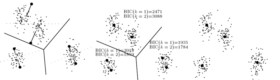
Figure 9: Framework for X-means [5]

Algorithm [6]

This algorithm further incorporates the merge step compared to $X$-means. It considers several internal validity indices $V(c)$, including BIC, Calinski and Harabasz index, Hartigan index, and so on, to decide when the split procedure or the merge procedure should stop. Algorithm [6] first splits clusters until validated to stop, and then continue to merge cluster until validated to stop (shown in Figure 10). In the merge step, the internal validity indices select two clusters with most average data sample similarity to merge.

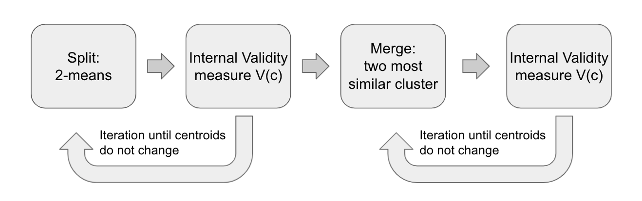
Figure 10: Framework for Algorithm [6]

Algorithm [7]

This method assumes knowledge of the ground truth cluster number $k$.This algorithm consists of three steps:

• Step 1: Run Lloyd’s $k$-means.

• Step 2: Split every cluster into $m$ clusters ($m=2,\cdots,M$) and calculate the ratio between successive $k$-means objectives $D$ .

  $$\rho(m)=D^{(m)}/D^{(m-1)},\quad\rho_{k}(m^{*})=\min\{\rho(m),m=2,...,M.\}$$

  This cluster will be split if $\rho_{k}(m^{*})$ is below some threshold.

• Step 3: Keep the split cluster that is furthest from neighboring voronoi regions and merge the rest of split clusters to neighboring voronoi regions.

This algorithm has very high computation complexity as it splits the sub-cluster several times with different split numbers and decide which split number is the most suitable one.

Algorithm [8]

This algorithm splits or merges cluster centers based on intra-cluster dissimilarity and inter-cluster dissimilarity defined below

$$d_{inter}=\left\|\ m_{i}-m_{j}\right\|^{2}$$

$$d_{intra}=\max\{\left\|\ m_{i}-x_{p}\right\|^{2}\}+\min\{\left\|\ m_{i}-x_{p}\right\|^{2}\}$$

here $m_{i}$ and $m_{j}$ represent the cluster centers of $i$-th and $j-th$ cluster, $x_{p}$ represent the data point in corresponding cluster. In addition, we define a thresold

$$\overline{d}=\frac{1}{A^{2}_{k}}\sum_{i=1}^{k}\sum_{j=1}^{k}\left\|\ m_{i}-m_{j}\right\|^{2}.$$ (19)

with $A^{2}_{k}$ being the number of pairwise cluster centers.

Then algorithm [8] can be formalized as the following:

• Split: iteratively update $\overline{d}$ and $d_{intra}$ and split the cluster until $d_{intra}<\overline{d}/2$

• Merge: iteratively update $\overline{d}$ and $d_{inter}$ and merge the clusters until $d_{inter}>\overline{d}/2$

Appendix D Different Detection Subroutines of FFkm

Table 10 and Table 11 show results from $100$ trials on the benchmark dataset for above variants of Fission-Fusion $k$-means(FFkm) and I-$k$-means$-$+. All three variants and I-$k$-means$-$+ obtain competitive results on most datasets, only making difference on heavily overlapped $S3$ and $S4$ dataset, where the theoretical characterization of local solutions no longer obtains.

Table 10: Success rate (%)

Data Set	I-$k$-means$-$+ [11]	SD+PD	SD+OI	TD+PD	TD+OI	RD+PD	RD+OI
A1	100	100	100	100	100	100	99(0.00)
A2	100	100	100	100	100	100	97(0.00)
A3	100	100	100	100	100	100	98(0.00)
S1	100	100	100	100	100	100	95(0.00)
S2	100	100	100	100	100	100	99(0.00)
S3	100	77(0.02)	89(0.00)	87(0.01)	96(0.00)	89(0.01)	92(0.01)
S4	93(0.00)	31(0.05)	39(0.04)	43(0.04)	90(0.01)	41(0.05)	77(0.02)
Unbalance	100	100	100	100	100	100	99(0.00)
Dim032	100	100	100	100	100	100	100
Birch1	100	100	100	100	100	100	100

Table 11: $\rho$-ratio

Data Set	I-$k$-means$-$+ [11]	SD+PD	SD+OI	TD+PD	TD+OI	RD+PD	RD+OI
A1	$1.00\pm 0.00$	$1.00\pm 0.00$	$1.00\pm 0.00$	$1.00\pm 0.00$	$1.00\pm 0.00$	$1.00\pm 0.00$	$1.00\pm 0.02$
A2	$1.00\pm 0.00$	$1.00\pm 0.00$	$1.00\pm 0.00$	$1.00\pm 0.00$	$1.00\pm 0.00$	$1.00\pm 0.00$	$1.01\pm 0.04$
A3	$1.00\pm 0.00$	$1.00\pm 0.00$	$1.00\pm 0.00$	$1.00\pm 0.00$	$1.00\pm 0.00$	$1.00\pm 0.00$	$1.00\pm 0.00$
S1	$1.00\pm 0.00$	$1.00\pm 0.00$	$1.00\pm 0.00$	$1.00\pm 0.00$	$1.00\pm 0.00$	$1.00\pm 0.00$	$1.03\pm 0.13$
S2	$1.00\pm 0.00$	$1.00\pm 0.00$	$1.00\pm 0.00$	$1.00\pm 0.00$	$1.00\pm 0.00$	$1.00\pm 0.00$	$1.01\pm 0.06$
S3	$1.01\pm 0.02$	$1.03\pm 0.05$	$1.01\pm 0.04$	$1.01\pm 0.04$	$1.00\pm 0.00$	$1.01\pm 0.04$	$1.01\pm 0.04$
S4	$1.01\pm 0.01$	$1.05\pm 0.04$	$1.05\pm 0.05$	$1.04\pm 0.04$	$1.01\pm 0.02$	$1.06\pm 0.07$	$1.03\pm 0.06$
Unbalance	$1.00\pm 0.00$	$1.00\pm 0.00$	$1.00\pm 0.00$	$1.00\pm 0.00$	$1.00\pm 0.00$	$1.00\pm 0.00$	$1.06\pm 0.63$
Dim032	$1.00\pm 0.00$	$1.00\pm 0.00$	$1.00\pm 0.00$	$1.00\pm 0.00$	$1.00\pm 0.00$	$1.00\pm 0.00$	$1.00\pm 0.00$
Birch1	$1.00\pm 0.00$	$1.00\pm 0.00$	$1.00\pm 0.00$	$1.00\pm 0.00$	$1.00\pm 0.00$	$1.00\pm 0.00$	$1.00\pm 0.00$

Appendix E Discussion the performance on a challenging Synthetic Dataset

This experiment also reflects the delicacy of the choice of detection subroutines for challenging datasets. Note that the proposed SD one-fit-many detection subroutine is explicitly designed to detect the one-fit-many association when the data clusters are slightly or moderately overlapped, where the theoretical characterization of local solution holds. To demonstrate this, we further test I-$k$-means$-$+ and FFkm (SD+PD) on a synthetic heavily unbalanced dataset shown in Figure 11. This unbalance dataset has eight clusters, whose centers follow the benchmark dataset [37]. We additionally up-sample the left three clusters to have $2000$ data points each, and the right five clusters to have $20000$ data points each. A: Lloyd’s $k$-means result of unbalance dataset. B-D: The iteration and final result of I-$k$-means$-$+. E-F: one-fit-many association and many-fit-one association detection of FFkm In this example, FFkm performs better to escape local minima in this unbalance dataset due to the choice of SD subroutine.

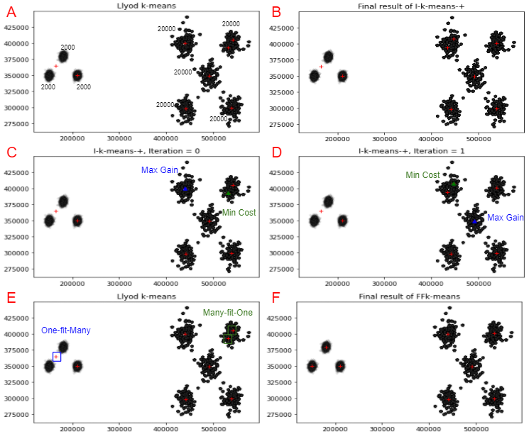
Figure 11: Comparefor the difference criterion of I-$k$-means$-$+ and FF$k$-means

Moreover, we executed Lloyd’s $k$-means, I-$k$-means$-$+ and FFkm(SD+PD) $100$ times in the above synthetic dataset shown in Table. 12. SR, AMR, $\rho$-ratio described in section 4.2. Time denotes the average execution time per run. Both I-$k$-means$-$+ and FFkm(SD+PD) perform much better than Lloyd’s $k$-means. Even though I-$k$-means$-$+ targets at decreasing object value (SSE) each iteration, it still runs into local minima with bigger objective value. On the other hand, FFkm(SD+PD) obtains better performance in this heavily unbalanced dataset and ensures to find the global solution (or ground truth) every run. At the same time, FFkm(SD+PD) is slightly faster than I-$k$-means$-$+, due to the relatively effecient many-fit-one association subroutine (minimum pairwise distance).

Table 12: Experiment result on synthetic dataset

Data Set	SR (%)	AMR	$\rho$-ratio (%)	sum of squared errors (SSE)	Time (s)
Lloyd	0	0.25	$1.27\pm 0.85$	$24847576040049\pm 167e^{11}$	0.0495
I-$k$-means$-$+	0	0.13	$1.01\pm 0.00$	$19763334088255\pm 276e^{8}$	0.4265
FFkm(SD+PD)	100	0.00	$1.00\pm 0.00$	$19603185158629\pm 0.00e^{0}$	0.4231

Appendix F Discussions on Computation Complexity

Moreover, we provide the average execution time from $100$ execution recordings shown in Table 13. As shown in the main theorem of this paper, the proposed algorithm takes polynomially many times as of Lloyd’s algorithm, while demonstrates superior accuracy compared to Lloyd’s algorithm. A large portion of the total computation time is spent on find one-fit-many association and many-fit-one association to avoid local minima and recover the ground truth centers.

Table 13: Computation Time in the Same Machine (seconds)

Data Set	Lloyd’s	$k$-means++	RD+PD	SD+PD	[11]	[7]	[8]	[5]
A1	0.0145	0.0214	0.1028	0.1031	0.0681	1.1306	0.2344	0.1849
A2	0.0177	0.0353	0.2464	0.2354	0.2618	2.1808	0.4194	0.5429
A3	0.0196	0.0493	0.5184	0.4698	0.7035	3.6021	0.7071	0.2756
S1	0.0158	0.0236	0.1263	0.0985	0.0717	0.9002	1.0352	1.1628
S2	0.0167	0.0243	0.1531	0.1243	0.0640	0.9185	2.0318	1.0084
S3	0.0174	0.0253	0.1341	0.1232	0.0617	0.9401	3.3655	0.3493
S4	0.0185	0.0264	0.1401	0.1237	0.0503	0.9190	3.2873	1.3176
Unbalance	0.0150	0.0206	0.1437	0.1176	0.0769	0.5452	0.4347	0.0888
Dim032	0.0999	0.2126	3.2161	2.6654	8.0708	4.9074	31.0177	1.2255
Birch1	0.1456	0.5827	14.5961	13.8357	7.7327	15.2493	4.2202	3.2935

Furthermore, two split-merge algorithm  [5, 8] with unknown number of initial clusters also posted in Table 13, with more details of algorithms to be found in Appendix C. For fair comparision, the inital cluster number k is setted as $k=k^{\star}$.

References

- [1] W. Qian, Y. Zhang, and Y. Chen, “Structures of spurious local minima in k-means,” IEEE Transactions on Information Theory, vol. 68, no. 1, pp. 395–422, 2021.
- [2] S. Lloyd, “Least squares quantization in pcm,” IEEE transactions on information theory, vol. 28, no. 2, pp. 129–137, 1982.
- [3] D. Arthur and S. Vassilvitskii, “k-means++: The advantages of careful seeding,” in Proceedings of the eighteenth annual ACM-SIAM symposium on Discrete algorithms, pp. 1027–1035, Society for Industrial and Applied Mathematics, 2007.
- [4] M. E. Celebi, H. A. Kingravi, and P. A. Vela, “A comparative study of efficient initialization methods for the k-means clustering algorithm,” Expert systems with applications, vol. 40, no. 1, pp. 200–210, 2013.
- [5] D. Pelleg, A. W. Moore, et al., “X-means: Extending k-means with efficient estimation of the number of clusters.,” in Icml, vol. 1, pp. 727–734, 2000.
- [6] M. Muhr and M. Granitzer, “Automatic cluster number selection using a split and merge k-means approach,” in 2009 20th International Workshop on Database and Expert Systems Application, pp. 363–367, IEEE, 2009.
- [7] F. Morii and K. Kurahashi, “Clustering by the k-means algorithm using a split and merge procedure,” in SCIS & ISIS SCIS & ISIS 2006, pp. 1767–1770, Japan Society for Fuzzy Theory and Intelligent Informatics, 2006.
- [8] J. Lei, T. Jiang, K. Wu, H. Du, G. Zhu, and Z. Wang, “Robust k-means algorithm with automatically splitting and merging clusters and its applications for surveillance data,” Multimedia Tools and Applications, vol. 75, no. 19, pp. 12043–12059, 2016.
- [9] P. Fränti and J. Kivijärvi, “Randomised local search algorithm for the clustering problem,” Pattern Analysis & Applications, vol. 3, no. 4, pp. 358–369, 2000.
- [10] P. Fränti and O. Virmajoki, “Iterative shrinking method for clustering problems,” Pattern Recognition, vol. 39, no. 5, pp. 761–775, 2006.
- [11] H. Ismkhan, “Ik-means-+: An iterative clustering algorithm based on an enhanced version of the k-means,” Pattern Recognition, vol. 79, pp. 402–413, 2018.
- [12] J. Sun, Q. Qu, and J. Wright, “Complete dictionary recovery over the sphere i: Overview and the geometric picture,” IEEE Transactions on Information Theory, vol. 63, no. 2, pp. 853–884, 2016.
- [13] J. Sun, Q. Qu, and J. Wright, “A geometric analysis of phase retrieval,” Foundations of Computational Mathematics, vol. 18, no. 5, pp. 1131–1198, 2018.
- [14] R. Ge, J. D. Lee, and T. Ma, “Matrix completion has no spurious local minimum,” Advances in Neural Information Processing Systems, pp. 2981–2989, 2016.
- [15] Y. Zhang, H.-W. Kuo, and J. Wright, “Structured local optima in sparse blind deconvolution,” IEEE Transactions on Information Theory, vol. 66, no. 1, pp. 419–452, 2020.
- [16] Q. Qu, Y. Zhai, X. Li, Y. Zhang, and Z. Zhu, “Analysis of the optimization landscapes for overcomplete representation learning,” arXiv preprint arXiv:1912.02427, 2019.
- [17] R. Ge and T. Ma, “On the optimization landscape of tensor decompositions,” Mathematical Programming, pp. 1–47, 2020.
- [18] Y. Zhang, Q. Qu, and J. Wright, “From symmetry to geometry: Tractable nonconvex problems,” arXiv preprint arXiv:2007.06753, 2020.
- [19] D. Jin, X. Bing, and Y. Zhang, “Unique sparse decomposition of low rank matrices,” Advances in Neural Information Processing Systems, 2021.
- [20] J. Xu, D. J. Hsu, and A. Maleki, “Global analysis of expectation maximization for mixtures of two gaussians,” in Advances in Neural Information Processing Systems, pp. 2676–2684, 2016.
- [21] C. Daskalakis, C. Tzamos, and M. Zampetakis, “Ten steps of em suffice for mixtures of two gaussians,” in Conference on Learning Theory, pp. 704–710, PMLR, 2017.
- [22] W. Qian, Y. Zhang, and Y. Chen, “Global convergence of least squares EM for demixing two log-concave densities,” in Advances in Neural Information Processing Systems, pp. 4795–4803, 2019.
- [23] K. Chaudhuri, S. Dasgupta, and A. Vattani, “Learning mixtures of gaussians using the k-means algorithm,” arXiv preprint arXiv:0912.0086, 2009.
- [24] C. Jin, Y. Zhang, S. Balakrishnan, M. J. Wainwright, and M. I. Jordan, “Local maxima in the likelihood of gaussian mixture models: Structural results and algorithmic consequences,” in Advances in neural information processing systems, pp. 4116–4124, 2016.
- [25] Y. Chen and X. Xi, “Likelihood landscape and local minima structures of Gaussian mixture models,” arXiv preprint arxiv:2009.13040, 2020.
- [26] D. Arthur and S. Vassilvitskii, “How slow is the k-means method?,” in Proceedings of the twenty-second annual symposium on Computational geometry, pp. 144–153, 2006.
- [27] G. H. Ball and D. J. Hall, “Promenade-an on-line pattern recognition system.,” tech. rep., STANFORD RESEARCH INST MENLO PARK CA, 1967.
- [28] N. Ueda, R. Nakano, Z. Ghahramani, and G. E. Hinton, “Smem algorithm for mixture models,” Neural Comput., vol. 12, pp. 2109–2128, Sept. 2000.
- [29] T. Kaukoranta, P. Franti, and O. Nevalainen, “Iterative split-and-merge algorithm for vector quantization codebook generation,” Optical Engineering, vol. 37, no. 10, pp. 2726–2732, 1998.
- [30] H. Frigui and R. Krishnapuram, “Clustering by competitive agglomeration,” Pattern recognition, vol. 30, no. 7, pp. 1109–1119, 1997.
- [31] P. Fränti and O. Virmajoki, “On the efficiency of swap-based clustering,” in International Conference on Adaptive and Natural Computing Algorithms, pp. 303–312, Springer, 2009.
- [32] B. Fritzke, “The lbg-u method for vector quantization–an improvement over lbg inspired from neural networks,” Neural Processing Letters, vol. 5, no. 1, pp. 35–45, 1997.
- [33] I. Katsavounidis, C.-C. J. Kuo, and Z. Zhang, “A new initialization technique for generalized lloyd iteration,” IEEE Signal processing letters, vol. 1, no. 10, pp. 144–146, 1994.
- [34] J. A. Hartigan and M. A. Wong, “Algorithm as 136: A k-means clustering algorithm,” Journal of the Royal Statistical Society. Series C (Applied Statistics), vol. 28, no. 1, pp. 100–108, 1979.
- [35] M. Astrahan, “Speech analysis by clustering, or the hyperphoneme method,” tech. rep., STANFORD UNIV CA DEPT OF COMPUTER SCIENCE, 1970.
- [36] F. Cao, J. Liang, and G. Jiang, “An initialization method for the k-means algorithm using neighborhood model,” Computers & Mathematics with Applications, vol. 58, no. 3, pp. 474–483, 2009.
- [37] P. Fränti and S. Sieranoja, “K-means properties on six clustering benchmark datasets,” Applied Intelligence, vol. 48, no. 12, pp. 4743–4759, 2018.
- [38] I. Kärkkäinen and P. Fränti, “Dynamic local search algorithm for the clustering problem,” Tech. Rep. A-2002-6, Department of Computer Science, University of Joensuu, Joensuu, Finland, 2002.
- [39] P. Fränti and O. Virmajoki, “Iterative shrinking method for clustering problems,” Pattern Recognition, vol. 39, no. 5, pp. 761–765, 2006.
- [40] P. Fränti, O. Virmajoki, and V. Hautamäki, “Fast agglomerative clustering using a k-nearest neighbor graph,” IEEE Trans. on Pattern Analysis and Machine Intelligence, vol. 28, no. 11, pp. 1875–1881, 2006.
- [41] M. Rezaei and P. Fränti, “Set-matching methods for external cluster validity,” IEEE Trans. on Knowledge and Data Engineering, vol. 28, no. 8, pp. 2173–2186, 2016.
- [42] P. Fränti, M. Rezaei, and Q. Zhao, “Centroid index: cluster level similarity measure,” Pattern Recognition, vol. 47, no. 9, pp. 3034–3045, 2014.