Beyond Gaussian pair fluctuation theory for strongly interacting Fermi gases II: The broken-symmetry phase

Abstract

We theoretically study the thermodynamic properties of a strongly interacting Fermi gas at the crossover from a Bardeen-Cooper-Schrieffer (BCS) superfluid to a Bose-Einstein condensate (BEC), by applying a recently outlined strong-coupling theory that includes pair fluctuations beyond the commonly-used many-body $T$-matrix or ladder approximation at the Gaussian level. The beyond Gaussian pair fluctuation (GPF) theory always respects the exact thermodynamic relations and recovers the Bogoliubov theory of molecules in the BEC limit with a nearly correct molecule-molecule scattering length. We show that the beyond-GPF theory predicts quantitatively accurate ground-state properties at the BEC-BCS crossover, in good agreement with the recent measurement by Horikoshi et al. in Phys. Rev. X 7, 041004 (2017). In the unitary limit with infinitely large $s$-wave scattering length, the beyond-GPF theory predicts a reliable universal energy equation of state up to 0.6$T_{c}$, where $T_{c}$ is the superfluid transition temperature at unitarity. The theory predicts a Bertsch parameter $\xi\simeq 0.365$ at zero temperature, in good agreement with the latest quantum Monte Carlo result $\xi=0.367(7)$ and the latest experimental measurement $\xi=0.367(9)$. We attribute the excellent and wide applicability of the beyond-GPF theory in the broken-symmetry phase to the reasonable re-summation of Feynman diagrams following a dimensional $\epsilon$-expansion analysis near four dimensions ($d=4-\epsilon$), which gives rise to accurate predictions at the second order $\mathcal{O}(\epsilon^{2})$. Our work indicates the possibility of further improving the strong-coupling theory of strongly interacting fermions based on the systematic inclusion of large-loop Feynman diagrams at higher orders $\mathcal{O}(\epsilon^{n})$ with $n\geq 3$.

I Introduction

There has been considerable effort over the last two decades to explore the properties of ultracold strongly interacting atomic Fermi gases Giorgini et al. (2008); Bloch et al. (2008); Randeria and Taylor (2014). In particular, the rapid advancement of experimental techniques has allowed for increasingly accurate measurements Nascimbène et al. (2010); Horikoshi et al. (2010); Ku et al. (2012); Horikoshi et al. (2017) of the universal thermodynamics of superfluid Fermi gases Ho (2004); Hu et al. (2007). This progress gives us access to understanding other less accessible or controllable strongly interacting Fermi systems, such as nuclear matter Lee and Schäfer (2006); Hen and et al (2014); van Wyk et al. (2018); Ohashi et al. (2020) and high-$T_{c}$ superconductors Loktev et al. (2001); Stajic (2017).

In greater detail, with the use of Feshbach resonances Chin et al. (2010) the interactions between fermions with unlike spins can be tuned to create weakly-coupled Cooper pairs and tightly-bound bosonic molecules, realizing a smooth crossover from a Bardeen-Cooper-Schrieffer (BCS) Fermi superfluid to a Bose-Einstein condensate (BEC) of bosons at sufficiently low temperatures Randeria and Taylor (2014). Near the Feshbach resonance, the $s$-wave scattering length $a_{s}$ becomes infinite and the system is uniquely defined by a single energy scale, the Fermi energy $E_{\rm F}$, or by the corresponding temperature scale $T_{\rm F}=E_{\rm F}/k_{B}$. In this unitary regime the system is scale invariant and its thermodynamic properties appear to be universal Ho (2004): all the thermodynamic functions are a function of a single parameter $T/T_{\rm F}$, independent of the microscopic details of the underlying interactions. As pointed out in Ref. Nikolic and Sachdev (2007), the universality of ultracold Fermi gases extends beyond the unitary regime to the BEC-BCS crossover. Interestingly, the general universality might be characterized by some universal relations, first derived by Shina Tan Tan (2008a, b, c). These relations reveal that the short-range and large-momentum behavior of dilute Fermi gases is encapsulated in the so-called contact parameter, which connects the thermodynamic properties of a fermionic system to its short-range behavior Braaten and Platter (2008); Zhang and Leggett (2009); Stewart et al. (2010); Kuhnle et al. (2010); Werner and Castin (2012); Braaten (2012). Due to the universality, the accurate determination of the thermodynamic properties of ultracold atomic Fermi gases would provide insight into other strongly interacting Fermi systems.

From a theoretical perspective, understanding ultracold strongly interacting fermions at finite temperatures is a grand challenge Randeria and Taylor (2014). As there is no small interaction parameter to perturbatively expand about, approximate perturbative methods in general are uncontrollable. Therefore, sophisticated quantum Monte Carlo (QMC) techniques are often used in the theoretical studies of strongly interacting Fermi systems. QMC calculations have been successfully applied to zero temperature superfluids Forbes et al. (2011); Gandolfi et al. (2011); Drut (2012), finite temperature superfluids Goulko and Wingate (2016); Jensen et al. (2020); Richie-Halford et al. (2020), and for systems above the superfluid transition in the normal state Van Houcke et al. (2012); Drut et al. (2012); Rossi et al. (2018). These QMC simulations are varied in their methodology, and with the difficulty in finding the zero-effective-range equation of state, the converged results differ between schemes. The most accurate simulation achieved so far is the calculation of the normal-state density or pressure equation of state of the unitary Fermi gas, through the bold diagrammatic Monte Carlo (BDMC) technique Van Houcke et al. (2012). This state-of-the-art theoretical result has a relative accuracy at the level of a few percent, comparable to the precision of the experimental data Ku et al. (2012); Van Houcke et al. (2012). However, the application of the intriguing BDMC approach to a superfluid Fermi gas is yet to be demonstrated.

Field theoretical methods offer an alternative route to calculate the thermodynamic properties without the difficulty of convergence. These include various diagrammatic many-body $T$-matrix theories within the ladder approximation Nozieres and Schmitt-Rink (1985); De Melo et al. (1993); Ohashi and Griffin (2003); Pieri et al. (2004); Chen et al. (2005); Liu and Hu (2005); Taylor et al. (2006); Hu et al. (2006); Haussmann et al. (2007); Diener et al. (2008); Hu et al. (2008); Watanabe et al. (2010); He et al. (2015); Mulkerin et al. (2016); Tajima et al. (2017); Mulkerin et al. (2017); Pini et al. (2019), the dimensional $\epsilon$-expansion Nishida and Son (2006); Arnold et al. (2007); Nishida and Son (2007); Nishida (2007), large-$N$ expansion Veillette et al. (2007); Nikolic and Sachdev (2007), and non-perturbative functional renormalization group approach Diehl et al. (2007); Boettcher et al. (2014). Focusing on the different many-body $T$-matrix theories, where the complete geometric series of ladder diagrams can be summed up. The difference lies on the degree of self-consistency taken in the diagrams, since either the bare non-interacting Green function or dressed interacting Green function can be used. In the normal state, the advantages of different $T$-matrix theories have been comparatively reviewed in Ref. Hu et al. (2008) (see also the recent extended study in Ref. Pini et al. (2019)). In this work, we are interested in the broken-symmetry superfluid phase below the critical temperature $T_{c}$.

As far as ultracold superfluid Fermi gases are concerned, the non-self-consistent $T$-matrix theory was first formulated by Ohashi and Griffin Ohashi and Griffin (2003) and by Pieri, Pisani and Strinati Pieri et al. (2004). A slightly modified version, in light of the seminal work by Nozières and Schmitt-Rink Nozieres and Schmitt-Rink (1985), was also developed shortly after Hu et al. (2006). The modification is equivalent to considering pair fluctuations at the Gaussian level De Melo et al. (1993); Diener et al. (2008), and therefore is termed as the Gaussian pair fluctuation (GPF) theory. Although in the normal state the modification only leads to fairly small changes Hu et al. (2008), it yields a non-trivial improvement for the superfluid equation of state Hu et al. (2006); Diener et al. (2008) due to the thermodynamic consistency in determining the number density (i.e., the number density calculated by using single-particle Green function or thermodynamic potential should be the same). On the other hand, a fully self-consistent $T$-matrix theory was developed by Haussmann and co-workers Haussmann et al. (2007), taking advantage of satisfying the Luttinger-Ward (LW) identity. Most recently, a partially self-consistent $T$-matrix theory was also considered by Tajima and co-workers Tajima et al. (2017). To ensure the crucial thermodynamic consistency in the superfluid phase, they proposed to first determine the chemical potential using the $T$-matrix diagrams, from which all the equations of state are then calculated through various exact thermodynamic relations Tajima et al. (2017).

In general, there is no a priori reason to justify the application of various many-body $T$-matrix theories, although the fully self-consistent LW theory seems to be more preferable in the literature. Naively, to quantitatively evaluate the many-body $T$-matrix theories in the superfluid phase, we may consider two useful criteria: (i) in the unitary limit the theory should provide a better explanation of the benchmark universal equation of state, which becomes available due to the increasingly accurate measurements of the unitary Fermi gas Nascimbène et al. (2010); Horikoshi et al. (2010); Ku et al. (2012); and (ii) in the BEC limit the theory should be able to recover a Bogoliubov theory of composite molecules with the correct molecular scattering length $a_{\rm M}\simeq 0.60a_{s}$ Petrov et al. (2004). For the first criterion, the self-consistent LW theory is clearly favored. For instance, it predicts a Bertsch parameter $\xi=0.360$ of a zero temperature unitary Fermi gas, which is close to the experimental result in the milestone measurement $\xi\simeq 0.376(4)$ Ku et al. (2012), contrasted with other many-body $T$-matrix predictions (i.e., $\xi=0.455$ from the non-self-consistent $T$-matrix Pieri et al. (2004), $\xi=0.401$ from the GPF Hu et al. (2006); Diener et al. (2008), and $\xi=0.381$ from the partially self-consistent $T$-matrix Tajima et al. (2017)). However, in the BEC limit the self-consistent LW theory gives an incorrect molecular scattering length $2a_{s}$ and thereby does not fulfill the second criterion. Actually, almost all the many-body $T$-matrix theories predict the same molecular scattering length $2a_{s}$ and violate the second criterion. The only exception is the GPF theory, which predicts $a_{\rm M}\simeq 0.57a_{s}$ Hu et al. (2006); Diener et al. (2008), a value very close to the exact result. The same is also true for a two-dimensional interacting Fermi gas He et al. (2015). The much-improved molecular scattering length from the GPF theory in both three and two dimensions might be qualitatively understood from the renormalization of the dispersion relation of the gapless Goldstone mode upon the change of energy scale Salasnich and Bighin (2015).

It is desirable to develop better field theoretical approaches, benchmarked against the above-mentioned two criteria. In this respect, the GPF theory could provide an ideal starting point. In a previous work Mulkerin et al. (2016), going beyond the Gaussian fluctuation approximation (or more broadly the many-body $T$-matrix ladder approximation) has been attempted for a strongly interacting Fermi gas in the normal state, motivated by the dimensional $\epsilon$-expansion studied in Refs. Nishida and Son (2006); Nishida (2007); Nishida and Son (2007); Arnold et al. (2007). One selects the important diagrams, which contribute the most near the upper critical dimension of four. In other words, a weighting factor is artificially assigned to the diagrams, according to the powers of $\epsilon=4-d$, although in the calculation the dimension $d\sim 4$ (i.e., $\epsilon\ll 1$ in the initial assumption) eventually one takes the realistic value of three, leading to $\epsilon=1$. The beyond-GPF theory in Ref. Mulkerin et al. (2016) explored the possibility of including all the diagrams up to the order $\mathcal{O}(\epsilon^{2})$ near four dimensions. When applied to calculate the universal equation of state of a unitary Fermi gas above the superfluid transition and compared with the benchmark experimental data Ku et al. (2012), the beyond-GPF theory shows excellent agreement down to the temperature $0.5T_{\rm F}$, better than the self-consistent LW theory Mulkerin et al. (2016). At high temperature above Fermi degeneracy, it also provides better agreement with the asymptotically exact third-order quantum virial expansion Liu et al. (2009).

In this work, we aim to apply the beyond-GPF theory to the broken-symmetry superfluid phase and calculate the low-temperature dependence of the chemical potential, energy, and Tan contact parameter throughout the BEC-BCS crossover. We critically examine its applicability at low temperatures by using the latest benchmark experimental measurements and the latest QMC simulations. At essentially zero temperature, we focus on the comparison with the experimental data obtained by Horikoshi et al. at the University of Tokyo Horikoshi et al. (2017). While for the universal equation of state in the unitary limit, we consider the most recent measurement by Li et al. at University of Science and Technology of China (USTC), Shanghai Branch Li et al. (2021). In both cases, we find excellent quantitative agreement. Further improvement of our beyond-GPF theory is possible, as the systematic inclusion of large-loop Feynman diagrams at higher orders $\mathcal{O}(\epsilon^{n})$ ($n\geq 3$) can be achieved by using, for example, the BDMC technique Van Houcke et al. (2012).

The paper is set out as follows. In Sec. II we briefly summarize the theoretical framework used and derive the thermodynamic potential within the beyond-GPF theory. In Sec. III we describe the thermodynamic properties of the BEC-BCS crossover at very low temperature. In Sec. IV we show the temperature dependence of the thermodynamic properties at unitarity. Finally, in Sec. V we summarize our results.

II Beyond Gaussian pair fluctuation theory

The theoretical framework of the beyond-GPF theory for an interacting Fermi gas in the normal state has been outlined in the work Mulkerin et al. (2016). In this section, we briefly review the key ideas of the beyond-GPF theory and extend it to the broken-symmetry superfluid phase.

A three-dimensional interacting Fermi gas at the BEC-BCS crossover is well described by the single-channel model Hamiltonian density for field operators $\psi_{\sigma}$ Hu et al. (2010),

$$\mathcal{H}=\sum_{\sigma}{\psi}^{\dagger}_{\sigma}(x)\mathcal{H}_{0}\psi_{\sigma}(x)+U_{0}{\psi}^{\dagger}_{\uparrow}(x){\psi}^{\dagger}_{\downarrow}(x)\psi_{\downarrow}(x)\psi_{\uparrow}(x),$$ (1)

where $\mathcal{H}_{0}=-\nabla^{2}/(2M)-\mu$, $M$ is the mass of fermions, and $\mu$ is the chemical potential. Throughout the work we shall use the notation $x=(\tau,\mathbf{x})$ and set the reduced Planck constant $\hbar=1$ and the volume $V=1$. We consider a contact interaction with strength $U_{0}<0$, which is known to have an ultraviolet divergence Bloch et al. (2008). This can be resolved by relating the bare contact interaction strength $U_{0}$ to the $s$-wave scattering length $a_{s}$ via,

$$\frac{M}{4\pi a_{s}}=\frac{1}{U_{0}}+\sum_{\mathbf{k}}\frac{1}{\mathbf{k}^{2}/M}.$$ (2)

A convenient method to calculate the thermodynamics of ultracold interacting Fermi gases is through the thermodynamic potential: $\Omega=-k_{{\rm B}}T\ln\mathcal{Z}$, where $T$ is the temperature, $\mathcal{Z}=\int\mathcal{D}\left[\psi,\bar{\psi}\right]e^{-S\left[\psi,\bar{\psi}\right]}$ is the partition function, and $\psi$ and $\bar{\psi}$ are independent Grassmann fields. The partition function is defined by the action and Hamiltonian in Eq. (1) via

$$S[\psi,\bar{\psi}]=\int_{0}^{\beta}d\tau\int d\mathbf{r}\left[\sum_{\sigma}\bar{\psi}_{\sigma}(x)\partial_{\tau}\psi_{\sigma}(x)+\mathcal{H}\right],$$ (3)

where $\beta=1/(k_{\rm B}T)$. In the strongly interacting regime we must go beyond the qualitatively reliable mean-field (MF) theory and include higher-order quantum fluctuations. Taking the Hubbard-Stratonovich transformation we write the action in terms of a bosonic field, $\Delta(\mathcal{Q})$, and expand about its saddle point $\Delta_{0}$, $\Delta(\mathcal{Q})=\Delta_{0}+\varphi_{\mathcal{Q}}$, where $\varphi_{\mathcal{Q}}$ is the field operator representing fluctuations. Here, we have used for short-hand notation $\mathcal{Q}=(i\nu_{n},\mathbf{q})$ and $\sum_{\mathcal{Q}}\equiv(k_{B}T/V)\sum_{i\nu_{n}}\sum_{\mathbf{q}}$, and $\nu_{n}=2n\pi/\beta$ ($n\in\mathbb{Z}$) are the bosonic Matsubara frequencies. After integrating out the Grassmann fields and taking a perturbative expansion of the bosonic action in orders of the fluctuation field, we have $\mathcal{S}_{{\rm eff}}\left[\Delta,\Delta^{*}\right]=\mathcal{S}_{{\rm MF}}^{(0)}+\mathcal{S}_{{\rm GF}}^{(2)}+\mathcal{S}^{(3)}+\mathcal{S}^{(4)}+\dots$, where $\mathcal{S}_{{\rm MF}}^{(0)}$ is the mean-field contribution, $\mathcal{S}_{{\rm GF}}^{(2)}$ is the Gaussian contribution, and $\mathcal{S}^{(n)}$ are higher order contributions Mulkerin et al. (2016). The conceptually simple picture of including fluctuations up to the Gaussian order captures the most relevant physics for strongly-coupled systems, by including the contributions from fermions and Cooper pairs. This GPF model provides a reasonable description of the BEC-BCS crossover in both three dimensions Hu et al. (2006, 2007); Diener et al. (2008); Tempere and Devreese (2012) and two-dimensions He et al. (2015); Mulkerin et al. (2017). However, in order to find a more accurate description of a strongly interacting Fermi gas, higher-order pair fluctuations beyond the Gaussian level need to be taken into the thermodynamic potential.

In previous work Mulkerin et al. (2016), motivated by the dimensional $\epsilon$-expansion Nishida and Son (2006); Arnold et al. (2007); Nishida and Son (2007); Nishida (2007) and re-interpreting the small dimensional parameter $\epsilon$ as the pair Green’s function, $\Gamma(\mathcal{Q})$, the thermodynamic potential beyond GPF up to order $\mathcal{O}(\epsilon^{2})$ was shown to be $\Omega=\Omega_{\rm MF}+\Omega_{\rm GF}+(\beta V)^{-1}\langle\mathcal{S}_{4}\rangle$, near the upper critical four dimensions. Here, the mean-field thermodynamic potential is given by,

$$\Omega_{\textrm{MF}}=\frac{\Delta^{2}}{U_{0}}+\sum_{\mathbf{k}}\left[\xi_{\mathbf{k}}-E_{\mathbf{k}}-\frac{2}{\beta}\ln\left(1+e^{\beta E_{\mathbf{k}}}\right)\right],$$ (4)

$\xi_{\mathbf{k}}=\mathbf{k}^{2}/(2M)-\mu$, $E_{\mathbf{k}}=\sqrt{\xi_{\mathbf{k}}^{2}+\Delta^{2}}$, and to ensure the gapless Goldstone mode, the pairing gap $\Delta$ should be calculated using the mean-field gap equation:

$$\frac{m}{4\pi a_{s}}+\sum_{\mathbf{k}}\left[\frac{1-2f\left(E_{\mathbf{k}}\right)}{2E_{\mathbf{k}}}-\frac{1}{\mathbf{k}^{2}/M}\right]=0,$$ (5)

with the Fermi distribution function $f(x)=\smash{1/(e^{\beta x}+1)}$. A significant advantage of our methodology is that the gap equation is calculated at the mean-field level and satisfies Goldstone’s theorem while still including quantum fluctuations. This is in sharp contrast to the self-consistent LW theory, where a running coupling constant should be assumed in order to satisfy the gapless condition Haussmann et al. (2007). The expression for the GPF thermodynamic potential is determined by integrating out the pairing fluctuation fields from the action, arriving at $\Omega_{\rm GF}=k_{B}T\sum_{\mathcal{Q}}\mathcal{F}\left(\mathcal{Q}\right)e^{i\nu_{n}0^{+}}$, where the function $\mathcal{F}\left(\mathcal{Q}\right)\equiv(1/2)\ln[-\Gamma^{-1}(\mathcal{Q})]$ can be rewritten as

$$\mathcal{F}=\frac{1}{2}\ln\left[1-\frac{M_{12}^{2}\left(\mathcal{Q}\right)}{M_{11}\left(\mathcal{Q}\right)M_{11}\left(-\mathcal{Q}\right)}\right]+\ln M_{11}\left(\mathcal{Q}\right).$$ (6)

The matrix elements $M_{11}$ and $M_{12}$ of the inverse pair correlation function $\Gamma^{-1}(\mathcal{Q})$ are given in Appendix A.

By extending the work Mulkerin et al. (2016) to the broken-symmetry phase, as detailed in Appendix A, the beyond Gaussian pair fluctuation contribution to the thermodynamic potential can be expressed by the three terms:

$$\frac{\langle\mathcal{S}^{(4)}\rangle}{\beta V}=\Omega^{(a)}+\Omega^{(b)}+\Omega^{(c)},$$ (7)

where,

$$\Omega^{(a)} =\sum_{\mathcal{K}}G_{11}^{(0)}(\mathcal{K})G_{11}^{(0)}(\mathcal{K})\Sigma_{11}^{(0)}(\mathcal{K})\Sigma_{11}^{(0)}(\mathcal{K}),$$

$$\Omega^{(b)} =\sum_{\mathcal{K}}G_{12}^{(0)}(\mathcal{K})G_{12}^{(0)}(\mathcal{K})\Sigma_{11}^{(0)}(\mathcal{K})\Sigma_{22}^{(0)}(\mathcal{K}),$$

$$\Omega^{(c)} =\sum_{\mathcal{K}\mathcal{Q}_{1}\mathcal{Q}_{2}}G_{12}^{(0)}(\mathcal{K})G_{11}^{(0)}(\mathcal{K}-\mathcal{Q}_{1})G_{12}^{(0)}(\mathcal{K}-\mathcal{Q}_{1}+\mathcal{Q}_{2})$$

$$\hskip 35.0pt\times G_{22}^{(0)}(\mathcal{K}+\mathcal{Q}_{2})\Gamma_{22}(\mathcal{Q}_{1})\Gamma_{22}(\mathcal{Q}_{2}).$$ (8)

Here the BCS Green’s function is given by $G^{(0)}(\mathcal{K})=[i\omega_{m}-\xi_{\mathbf{k}}\tau_{3}+\Delta\tau_{1}]^{-1}$, and $\tau_{i}$ are the Pauli matrices. The self-energy $\Sigma^{(0)}$, arising from the beyond GPF diagrams, takes the form Mulkerin et al. (2016),

$$\Sigma_{\alpha\alpha^{\prime}}^{(0)}(\mathcal{K}) =\sum_{\mathcal{Q}}\Gamma_{\alpha\alpha^{\prime}}(\mathcal{Q})G_{\alpha\alpha^{\prime}}^{(0)}(\mathcal{Q}-\mathcal{K}),$$ (9)

for $\{\alpha,\alpha^{\prime}\}=\{1,2\}$. We use for short-hand notation $\mathcal{K}=(i\omega_{m},\mathbf{k})$ and $\sum_{\mathcal{K}}\equiv(k_{B}T/V)\sum_{i\omega_{m}}\sum_{\mathbf{k}}$, and $\omega_{m}=(2m+1)\pi/\beta$ ($m\in\mathbb{Z}$) are the fermionic Matsubara frequencies.

For the sake of clarity, we leave the technical details of the beyond-GPF calculations to Appendix A. In our calculations, the number density is determined through the thermodynamic potential by $n=-\partial\Omega/\partial\mu$, which fixes the Fermi wavevector $k_{\rm F}=(3\pi^{2}n)^{1/3}$. We self-consistently converge the number density through adjusting the chemical potential and order parameter using Eq. (5). The temperature scale and energy scale are defined through $k_{\rm B}T_{\rm F}=\epsilon_{\rm F}=k^{2}_{\rm F}/2M$. The dimensionless interaction parameter is given by $1/(k_{\rm F}a_{s})$.

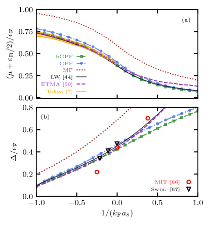
Figure 1: The chemical potential (a) and the superfluid gap parameter (b) in units of the Fermi energy are plotted as a function of the dimensionless interaction parameter $1/(k_{\rm F}a_{s})$ at the reduced temperature $T/T_{\rm F}=0.06$. For the chemical potential, we have subtracted half the bound state energy, $-\varepsilon_{B}/2=-1/(2Ma_{s}^{2})$. We plot the predictions from different theories: mean-field (brown dotted line), GPF (blue line with circles) Hu et al. (2006), partially self-consistent or extended $T$-matrix (ETMA, purple dashed line) Tajima et al. (2017), fully self-consistent LW theory (black solid line) Haussmann et al. (2007), and beyond-GPF calculation (green line with squares). We compare the different theoretical predictions with the experimental data from University of Tokyo Horikoshi et al. (2017) (orange solid line; $T/T_{\rm F}\simeq 0.06$). For the superfluid gap parameter, we instead compare the theories with the experimental data from MIT Schirotzek et al. (2008) (red hexagons) and Swinburne University of Technology Hoinka et al. (2017) (black triangles; $T/T_{\rm F}\simeq 0.09$).

III BEC-BCS crossover at very low temperatures

To begin our discussion of the beyond-GPF results, we first consider the chemical potential and superfluid gap parameter at the BEC-BCS crossover as a function of the dimensionless interaction parameter $-1\leq 1/k_{\rm F}a_{s}\leq+1$ at the temperature $T/T_{\rm F}=0.06$. This is the temperature set by the experiment on the ground-state thermodynamics at the University of Tokyo Horikoshi et al. (2017). As in the experiment, we expect the temperature dependence below $T/T_{\rm F}=0.06$ to not be significant and we discuss essentially the ground-state properties of the BEC-BCS crossover. Here, we focus on the comparison of different strong-coupling theories with respect to the benchmark experimental data from Tokyo group Horikoshi et al. (2017), as reported in Fig. 1.

As we already mentioned in the Introduction, the GPF, extended $T$-matrix ETMA, and fully self-consistent LW theories all belong to the many-body $T$-matrix theories within the ladder approximation, but differ in the degree of self-consistency adopted in the ladder diagrams. For the chemical potential in Fig. 1(a), in comparison to the benchmark Tokyo data on the BCS side (i.e., $-1\leq 1/k_{\rm F}a_{s}\leq 0$), all the $T$-matrix theories show good agreements, much better than the mean-field prediction shown in the brown dotted line. In particular, both the ETMA and LW theories agree well with the experimental results, with discrepancies smaller than the error bar of data. The simplest non-self-consistent $T$-matrix theory, the GPF theory, seems to provide a worse agreement on the BCS side, as its prediction lies systematically above the experimental data. This weakness can be overcome by including the higher-order diagrams beyond the GPF approximation. Indeed, within our scheme of the inclusion of pair fluctuations at the second order $\mathcal{O}(\epsilon^{2})$ in the $\epsilon$-expansion, we find that the beyond-GPF theory agrees with the Tokyo data within the experimental uncertainty.

On the BEC side of the Feshbach resonance (i.e., $1/k_{\rm F}a_{s}\geq 0$), recent experimental data is not available. However, it is known analytically that both the ETMA Tajima et al. (2017) and LW theories Haussmann et al. (2007) fail to predict the correct molecular scattering length $a_{\rm M}$ between two composite bosons. This failure can be partly seen from the chemical potential given by the ETMA theory, which slightly shifts up at large $1/(k_{F}a_{s})$ compared with other theories. In contrast, the GPF theory provides an approximately accurate molecular scattering length $a_{\rm M}\simeq 0.57a_{s}$ Hu et al. (2006); Diener et al. (2008). Although we can not obtain analytically the molecular scattering length in the beyond-GPF theory, it is readily seen that, towards the BEC limit both the GPF and beyond-GPF theories nearly predict the same chemical potential. This strongly indicates that the pair fluctuations at the second order $\mathcal{O}(\epsilon^{2})$ becomes less important in the BEC limit and therefore does not contribute to the molecular scattering length. As a result, the beyond-GPF theory inherits the accurate molecular scattering length of the GPF theory in the BEC limit. Therefore, among the different strong-coupling theories considered in Fig. 1, it seems that the beyond-GPF theory somehow provides overall the best prediction at the BEC-BCS crossover for the low-temperature thermodynamics. Further measurements of thermodynamics on the BEC side will be useful to examine this anticipation.

Another useful experimental comparison comes from dynamical measurements of the superfluid gap parameter through the radio-frequency spectroscopy Schirotzek et al. (2008) or Bragg spectroscopy Hoinka et al. (2017). Fig. 1(b) plots the gap parameters predicted by different strong-coupling theories and compares them to the experimental results from MIT Schirotzek et al. (2008) and Swinburne University of Technology Hoinka et al. (2017). The slight but systematic improvement of the beyond-GPF theory over the simplest GPF theory is clearly visible. On the BCS side, the beyond-GPF prediction agrees well with the results from the ETMA and LW theories. On the BEC side, the discrepancies among the different theories simply follows the different chemical potential as seen from Fig. 1(a), since the gap parameter is calculated by using the mean-field gap equation at given chemical potential. The only exception is the fully self-consistent LW theory Haussmann et al. (2007), where a running coupling constant is used to ensure the gapless condition for the Goldstone phonon mode, so the gap parameter no longer follows the mean-field gap equation. This explains why the ETMA and LW theories predict similar gap parameter on the BEC side, despite the different chemical potential. We note that, at current stage the spectroscopic measurement of the gap parameter in general has less accuracy than the thermodynamic measurement as shown in Fig. 1(a). Thus, the comparison of the theories to the experimental data for the gap parameter given in Fig. 1(b) is just indicative. We anticipate that future measurement of the gap parameter with novel high-resolution Bragg spectroscopy Li et al. (2021) may provide us a stringent test of many-body strong-coupling theories.

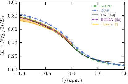
Figure 2: The internal energy in units of $E_{0}=(3/5)N\epsilon_{\rm F}$ relative to the bound state energy is plotted as a function of the interaction parameter $1/(k_{\rm F}a_{s})$ at the reduced temperature $T/T_{\rm F}=0.06$. We plot the energy calculated from the GPF (blue dash-dotted), extended $T$-matrix ETMA (purple dashed), fully self-consistent LW (black solid) and beyond-GPF theories (green dashed). The experimental data on energy is from University of Tokyo in Ref. Horikoshi et al. (2017) (orange solid line) at the same reduced temperature $T/T_{\rm F}\simeq 0.06$.

We consider next the internal energy at the BEC-BCS crossover. An advantage of our beyond-GPF calculation is that, once the chemical potential is found for a given interaction strength, we can calculate straightforwardly various thermodynamic quantities. For example, the internal energy is found from the relation:

$$E=\Omega+TS+\mu N,$$ (10)

where $S=(-\partial\Omega/\partial T)_{\mu}$ is the entropy. We plot the internal energy in Fig. 2 in units of $E_{0}=(3/5)N\epsilon_{\rm F}$ relative to the bound-state energy of $N/2$ molecules, $-N\varepsilon_{B}/2=-N/(2Ma_{s}^{2})$, as a function of $1/k_{\rm F}a_{s}$ at the temperature $T/T_{\rm F}=0.06$. The predictions from the different theories, the GPF (blue dash-dotted), extended $T$-matrix (purple dashed), fully self-consistent LW (black solid) and beyond-GPF (green solid), are compared with the experimental data from Ref. Horikoshi et al. (2017). Once again, on the BCS side we see the improvement of the GPF prediction with the inclusion of the higher-order non-Gaussian pair fluctuations and the excellent agreement between experiment and theory. Towards the deep BEC limit, the non-Gaussian pair fluctuations become less important and we find that both the GPF and beyond-GPF theories tend to give the same internal energy. The fully self-consistent LW theory predicts a slightly higher internal energy than the beyond-GPF theory in the BEC limit. This is in line with the fact that the LW theory does not give the correct molecular scattering length: it predicts a mean-field molecular scattering length $a_{\rm M}=2a_{s}$ Haussmann et al. (2007), about three times larger than the exact value of $a_{\rm M}\simeq 0.6a_{s}$ Petrov et al. (2004).

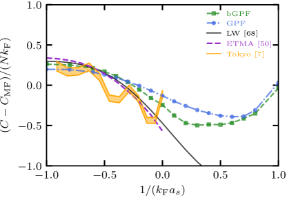
Figure 3: Tan’s contact parameter in units of $Nk_{\rm F}$ relative to the mean-field prediction is plotted as a function of the interaction parameter $1/(k_{\rm F}a_{s})$ at the reduced temperature $T/T_{\rm F}=0.06$. We compare the theoretical predictions from the GPF (blue dash-dotted), extended $T$-matrix ETMA (purple dashed), fully self-consistent LW Haussmann et al. (2009) (black solid) and beyond-GPF theories (green dashed), with the experimental results from University of Tokyo in Ref. Horikoshi et al. (2017) (orange solid line) at the same reduced temperature $T/T_{\rm F}\simeq 0.06$.

Another important thermodynamic quantity is Tan’s contact parameter $C$, which determines the universal short-range, large-momentum and high-energy behavior of the many-body system Tan (2008a, b, c). From the adiabatic relation in the grand canonical ensemble Hu et al. (2011), the contact is related to the change in the thermodynamic potential as the interatomic interaction varies:

$$-\left[\frac{\partial\Omega}{\partial(a_{s}^{-1})}\right]_{\mu,T}=\frac{C}{4\pi M}.$$ (11)

Figure 3 shows the contact in units of $Nk_{\rm F}$ as a function of the interaction parameter $1/k_{\rm F}a_{s}$. The mean-field contribution has been subtracted, in order to highlight the difference between theories. For comparison, we show also the experimental data from Horikoshi et al. (2017). However, this comparison does not serve as an independent benchmark examination of the different theories, since the experimental data are derived from the measured internal energy and are not from other independent spectroscopic measurements such as those in Ref. Sagi et al. (2015). On the BCS side, there are good agreements between theories, as we already see in the chemical potential, gap parameter and internal energy. On the BEC side, we find that the GPF and beyond-GPF theories consistently predict a larger contact parameter than the LW theory. This is merely a reflection of the difference in the internal energy that we have discussed earlier.

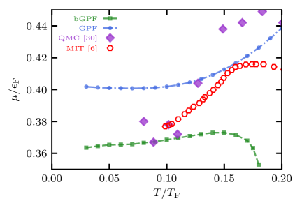
Figure 4: The chemical potential in units of the Fermi energy $\epsilon_{\rm F}$ is plotted as a function of the reduced temperature in the unitary limit, $1/(k_{\rm F}a_{s})=0$. These predictions are calculated by using the GPF theory (blue dash-dotted), beyond-GPF theory (green dashed), and lattice QMC from Ref. Goulko and Wingate (2016) (purple diamonds). We compare the theoretical results with the experimental data from MIT in Ref. Ku et al. (2012) (red hexagons).

IV Universal thermodynamics of a unitary Fermi gas

We now turn our attention to the temperature dependence of thermodynamic properties of a unitary Fermi gas and fix the $s$-wave scattering length to the unitary limit $1/(k_{\rm F}a_{s})=0$. In this limit, the interacting Fermi gas becomes scale invariant and all the thermodynamic functions can be expressed as a single function of the reduced temperature $T/T_{F}$. This unique advantage greatly simplifies the measurements of the equations of state and also improves the accuracy of experimental data. Universal thermodynamic function of the unitary Fermi gas have now been measured with unprecedented accuracy Ku et al. (2012); Li et al. (2021), with the characteristic lambda transition clearly revealed in the specific heat. Here, we focus on the comparison of the GPF and beyond-GPF theories with the latest experiment carried out at USTC Shanghai Li et al. (2021). This measurement benefits from a large homogeneous Fermi gas trapped in a box-potential and a novel high-resolution Bragg spectroscopy for the isentropic speed of sound Li et al. (2021). As a result, the experiment removes the local density approximation assumed in the previous measurement Ku et al. (2012). We also consider the comparison of the GPF and beyond-GPF theories with the latest available QMC simulations Goulko and Wingate (2016); Jensen et al. (2020).

We first plot the chemical potential as a function of the reduced temperature at unitarity in Fig. 4, which is calculated using the GPF (blue dash-dotted) and beyond-GPF theories (green dashed). As we approach zero temperature the Fermi surface becomes sharp, and in our numerical calculations accuracy becomes worse at very low temperatures. Therefore, we restrict ourselves to temperatures $T/T_{\rm F}\geq 0.03$. We compare the two theoretical predictions with the lattice QMC in Ref. Goulko and Wingate (2016) (purple diamonds) and the experimental chemical potential measured in Ref. Ku et al. (2012).

At low temperature $T/T_{\rm F}<0.1$, the GPF theory overestimates the chemical potential. We find instead that the beyond-GPF prediction is consistent with either the experimental result of Ref. Ku et al. (2012) or the finite-temperature QMC simulation Goulko and Wingate (2016). However, if we further increase temperature, the beyond-GPF theory seems to break down, presumably due to large critical thermal fluctuations close to the superfluid phase transition. This is clearly indicated by a maximum at $T/T_{\rm F}\simeq 0.15$ in the beyond-GPF chemical potential. The chemical potential continues to decrease for higher temperatures. We are not able to determine the superfluid transition temperature within the beyond-GPF theory. The beyond-GPF chemical potential shown in Fig. 4 is too large to yield a vanishing gap parameter. To locate the superfluid transition temperature, it might be useful to calculate the superfluid density using the beyond-GPF theory in future work.

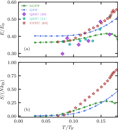
Figure 5: (a) The internal energy of a unitary Fermi gas is plotted as a function of the reduced temperature in units of an ideal gas energy, $E_{0}=(3/5)N\epsilon_{\rm F}$. We show the predictions from the GPF (blue circles), beyond-GPF (green squares), lattice QMC from Ref. Goulko and Wingate (2016) (purple diamonds) and auxiliary-field QMC from Ref. Jensen et al. (2020) (light-blue pentagons). We also compare the predictions with the experimental results from UTSC-Shanghai (brown stars) Li et al. (2021). (b) The entropy of a unitary Fermi gas is plotted as a function of reduced temperature in units $Nk_{\rm B}$ for the GPF (blue circles) and beyond-GPF calculations (green squares), and the experimental data from UTSC-Shanghai (brown stars) Li et al. (2021).

We now consider the internal energy, which at unitarity obeys the well-known scaling relation $E=-2\Omega/3$ Ho (2004); Nascimbène et al. (2010). In Fig. 5(a) we plot the internal energy in units of the ideal-gas energy at zero temperature $E_{0}=(3/5)N\epsilon_{\rm F}$ as a function of the reduced temperature. We compare the beyond-GPF energy (green dashed) to the theoretical predictions of the GPF theory (blue dash-dotted), lattice QMC results from Ref. Goulko and Wingate (2016) (purple diamonds) and auxiliary-field QMC results from Ref. Jensen et al. (2020) (light-blue pentagons), and experimental data from UTSC Shanghai Li et al. (2021) (brown stars). The internal energy calculated from our beyond-GPF theory agrees well with both QMC results and the experimental data in the low temperature regime. In particular, it is remarkable that at temperatures $T/T_{\rm F}<0.1$ the beyond-GPF energy exactly overlaps with the experimental data. The unitary Fermi gas can be related to the ideal Fermi gas at zero temperature via the Bertsch parameter, i.e., $E(T=0)=\xi E_{0}$. We find that the beyond-GPF theory predicts a Bertsch parameter $\xi\simeq 0.365$, in excellent agreement with the zero-temperature QMC $\xi=0.367(7)$ found in Ref. Jensen et al. (2020) and the experimental measurement $\xi=0.367(9)$ in Ref. Li et al. (2021). As the temperature increases above $T/T_{\rm F}=0.1$, we see the beyond-GPF energy starts to deviate from the benchmark experimental data. Indeed, near the critical temperature $T_{c}\simeq 0.17T_{\rm F}$, accurate theoretical predictions of the internal energy are notoriously difficult to obtain. This is partly indicated by the uncertainty of the two QMC results. Therefore, in order to accurately account for the experimental data, even the most advanced QMC simulations need to be improved.

In Fig. 5(b) we report the entropy in units of $Nk_{\rm B}$ as a function of the reduced temperature at unitarity. In the low temperature regime (i.e., $T/T_{\rm F}<0.1$), once again we find the excellent agreement between the beyond-GPF theory and the experiment. As the temperature increases, however, the beyond-GPF theory turns out to strongly under-estimate the entropy.

Figure 6: Tan’s contact parameter of a unitary Fermi gas in units of $Nk_{\rm F}$ is plotted as a function of the reduced temperature for the GPF (blue dash-dotted) and beyond-GPF calculations (green dashed), finite-temperature auxiliary-field QMC Jensen et al. (2020) (light-blue pentagons) and zero-temperature diffusion QMC simulations Gandolfi et al. (2011) (golden star). For comparison, we show also the early experimental result from Ref. Laurent et al. (2017) (purple cross) and the latest measurements from Ref. Mukherjee et al. (2019) (red hexagons) and Ref. Carcy et al. (2019) (black triangles).

Finally, we show in Fig. 6 Tan’s contact parameter in units of $Nk_{\rm F}$ as a function of the reduced temperature and compare the predictions of the GPF and beyond-GPF theories to several QMC calculations and experimental results. Our new calculation of the beyond-GPF theory (green dashed) systematically improves the earlier GPF result in Ref. Hu et al. (2011). As a consequence, in the low temperature regime the beyond-GPF prediction now seems to be able to smoothly connect to the various experimental data, from École Normale Supérieure (ENS) Laurent et al. (2017) (brown cross), MIT Mukherjee et al. (2019) (red hexagons) and Swinburne University of Technology Carcy et al. (2019) (black triangle). As the critical temperature is approached, the contact parameter given by the beyond-GPF theory does not decrease as sharply as the experimental results, since the theory fails to include strong thermal fluctuations in this critical temperature regime.

It is evident from Figs. 4, 5 and 6 that, although the beyond-GPF theory does not agree with the experimental data close to the superfluid transition, it is able to provide a quantitative explanation of the experimental results below the temperature $T<0.1T_{\rm F}\simeq 0.6T_{c}$. This accurate low-temperature description might be useful in understanding the thermodynamics of strongly interacting fermions at the intermediate low temperature regime, which may become difficult to address by both experiments (due to the less efficient thermometry) and QMC simulations (due to the rapid increase in simulation time at low temperatures).

V Conclusion

In summary, we have performed numerical calculations of the thermodynamics of a strongly interacting Fermi superfluid in the broken-symmetry phase, by using a recently developed strong-coupling theory that includes pair fluctuations beyond the standard Gauss approximation Mulkerin et al. (2016). We have critically examined the applicability of the beyond-GPF (Gaussian pair fluctuation) theory, by comparing its predictions for various equations of state and Tan’s contact parameter with the most recent experimental measurements and the latest quantum Monte Carlo simulations. On the BCS side and in the unitary limit, we find that the beyond-GPF theory is quantitatively reliable at low temperature. In particular, in the unitary limit, it predicts very a accurate chemical potential, energy, entropy and contact parameter. The beyond-GPF also leads to a Bertsch parameter that is in excellent agreement with the latest experiment Li et al. (2021) and Monte Carlo calculation Jensen et al. (2020). It is reasonable to believe that the beyond-GPF theory is also quantitatively reliable on the BEC side at low temperature and future experimental measurements on the low-temperature thermodynamics in the BEC regime would be useful to check this anticipation.

By combining the previous results for a normal, strongly interacting Fermi gas Mulkerin et al. (2016), we conclude that the beyond-GPF theory is a powerful tool in either low-temperature regime or high-temperature regime. In the former case, quantum fluctuations are stabilized by the pairing gap parameter; while in the latter, thermal fluctuations are significantly suppressed. In the unitary limit, the two temperature regimes are roughly given by $T<0.1T_{F}\simeq 0.6T_{c}$ and $T>0.5T_{F}$, respectively, where $T_{F}$ is Fermi degenerate temperature and $T_{c}\simeq 0.17T_{F}$ is the superfluid transition temperature at unitarity.

In the intermediate temperature regime (i.e., $0.1T_{F}\leq T\leq 0.5T_{F}$ for a unitary Fermi gas), the beyond-GPF theory needs to be improved to capture the strong thermal fluctuations near the superfluid transition. As the current beyond-GPF framework is built on the dimensional $\epsilon$-expansion, an immediate extension of our work is to carry out the beyond-GPF calculations near four dimensions with $d=4-\epsilon$, where the small parameter $0<\epsilon\ll 1$ and the large thermal fluctuations near the critical temperature can therefore be suppressed. We may then obtain the universal thermodynamic function such as $f_{E}\left(T/T_{F}\right)=E/E_{0}$ up to the second order $\mathcal{O}(\epsilon^{2})$. This naturally extends the earlier zero-temperature second-order $\epsilon$-expansion calculations in Ref. Arnold et al. (2007) to finite temperatures. In more general terms, we may pick the Feynman diagrams at higher orders $\mathcal{O}(\epsilon^{n})$ with $n\geq 3$. The systematic inclusion of the higher-order diagrams may greatly shrink the temperature window near the superfluid transition, where the beyond-GPF theory fails.

Appendix A Calculation details on the beyond Gaussian pair fluctuation theory

In this appendix, we present the full matrix elements for the GPF theory and technical details on the GPF and beyond-GPF calculations.

A.1 GPF

The thermodynamic potential including up to Gaussian fluctuations is $\Omega=\Omega_{\rm MF}+\Omega_{\rm GF}$ Hu et al. (2006); Diener et al. (2008), where $\Omega_{\rm MF}$ is the mean-field contribution and $\Omega_{\rm GF}=k_{B}T\sum_{\mathcal{Q}}\mathcal{F}\left(\mathcal{Q}\right)e^{i\nu_{n}0^{+}}$ the Gaussian fluctuation contribution, where

$$\mathcal{F}\left(\mathcal{Q}\right)=\frac{1}{2}\ln\left[1-\frac{M_{12}^{2}\left(\mathcal{Q}\right)}{M_{11}\left(\mathcal{Q}\right)M_{11}\left(-\mathcal{Q}\right)}\right]+\ln M_{11}\left(\mathcal{Q}\right).$$ (12)

Here, $\mathcal{Q}=(i\nu_{n},\mathbf{q})$ and $M_{11}(\mathcal{Q})$ and $M_{12}(\mathcal{Q})$ are the matrix elements of the inverse pair Green function $\Gamma^{-1}(\mathcal{Q})$ at finite temperatures and take the form Hu et al. (2006); Diener et al. (2008),

$$M_{11}(\mathcal{Q}) = \frac{1}{U_{0}}+\sum_{\mathbf{k}}\left[u_{+}^{2}u_{-}^{2}\frac{1-f_{+}-f_{-}}{i{\nu}_{n}-E_{+}-E_{-}}-u_{+}^{2}v_{-}^{2}\frac{f_{+}-f_{-}}{i\nu_{n}-E_{+}+E_{-}}+v_{+}^{2}u_{-}^{2}\frac{f_{+}-f_{-}}{i\nu_{n}+E_{+}-E_{-}}-v_{+}^{2}v_{-}^{2}\frac{1-f_{+}-f_{-}}{i{\nu}_{n}+E_{+}+E_{-}}\right],$$

$$M_{12}(\mathcal{Q}) = \sum_{\mathbf{k}}\left(u_{+}v_{+}u_{-}v_{-}\right)\left[-\frac{1-f_{+}-f_{-}}{i\nu_{n}-E_{+}-E_{-}}-\frac{f_{+}-f_{-}}{i\nu_{n}-E_{+}+E_{-}}+\frac{f_{+}-f_{-}}{i\nu_{n}+E_{+}-E_{-}}+\frac{1-f_{+}-f_{-}}{i\nu_{n}+E_{+}+E_{-}}\right],$$ (13)

where $M_{21}(\mathcal{Q})=M_{12}(\mathcal{Q})$ and $M_{22}(\mathcal{Q})=M_{11}(-\mathcal{Q})$. We note that, the short-hand notations $E_{\pm}=E_{\mathbf{k}\pm\mathbf{q}/2}$, $f_{\pm}^{\left(\pm\right)}=f(E_{\mathbf{k}\pm\mathbf{q}/2}^{\pm})$, $u_{\pm}^{2}=(1+\xi_{\mathbf{k}\pm\mathbf{q}/2}/E_{\mathbf{k}\pm\mathbf{q}/2})/2$, and $v_{\pm}^{2}=1-u_{\pm}^{2}$ are used.

Although it is straight forward to write down the GPF thermodynamic potential, in general $\Omega_{\rm GF}$ is difficult to solve numerically at finite temperatures. The bosonic Matsubara frequency sum $\sum_{i\nu_{n}}\mathcal{F}\left(i\nu_{n},\mathbf{q}\right)$ is divergent and we need to add an infinitesimal controlling factor $e^{i\nu_{n}\eta}$ with $\eta\rightarrow 0^{+}$ to ensure the convergence. At zero temperature, we may rewrite the summation into an integral, due to the fact that the vertex function $\Gamma(\mathcal{Q})$ does not have poles on the real axis for positive values Diener et al. (2008). However, this is no longer true at finite temperatures. If one uses the analytic continuation as in the seminal work Nozieres and Schmitt-Rink (1985), the numerical calculation then becomes extremely complicated Hu et al. (2006). The numerical difficulty can be avoided by splitting the Matsubara sum into two parts Mulkerin et al. (2017); Tempere et al. (2008),

$$\sum_{n}\mathcal{F}_{\eta}\left(i\nu_{n},\mathbf{q}\right)=\sum_{\left|n\right|>n_{0}}\mathcal{F}_{\eta}\left(i\nu_{n},\mathbf{q}\right)+\sum_{n=-n_{0}}^{n_{0}}\mathcal{F}_{\eta}\left(i\nu_{n},\mathbf{q},\right)$$ (14)

for arbitrary positive integer $n_{0}$. Here, $\mathcal{F}_{\eta}(i\nu_{n},\mathbf{q})\equiv\mathcal{F}(i\nu_{n},\mathbf{q})e^{i\nu_{n}\eta}$. We simplify the first divergent term by closing the contour at finite imaginary constant, off the real axis, i.e. for finite $\gamma=(2n_{0}+1)\pi/\beta$,

$$\frac{1}{\beta}\sum_{\left|n\right|>n_{0}}\mathcal{F}_{\eta}\left(i\nu_{n},\mathbf{q}\right)=-\frac{1}{\pi}\int_{-\infty}^{+\infty}d\omega\frac{\textrm{Im}\mathcal{F_{\eta}}\left(\omega+i\gamma,\mathbf{q}\right)}{e^{\beta\omega}+1}.$$ (15)

The second term is convergent and can be calculated directly at bosonic Matsubara frequencies $i\nu_{n}$. The contribution to $\Omega_{\textrm{GF}}$ at a given wavevector $\mathbf{q}$ can then be obtained by using Eqs. (14) and (15). We have checked that this numerical method is consistent with previous theoretical calculations in Ref. Hu et al. (2006) and is independent of the choice of $n_{0}$, as it should be.

A.2 Beyond GPF

The expression of the beyond Gaussian fluctuation contribution to the thermodynamic potential is determined with the method detailed in Ref. Mulkerin et al. (2016). Re-interpreting the $\epsilon$-expansion found by Refs. Nussinov and Nussinov (2006); Nishida and Son (2006); Nishida (2007) in orders of the vertex function $\Gamma$, the $\mathcal{S}^{(4)}$ contribution to the thermodynamic potential is

$$\frac{\mathcal{S}^{(4)}}{\beta V}=\frac{1}{4}\sum\mathrm{Tr}_{\sigma}{G}_{0}(\mathcal{K})\left(\begin{array}[]{cc}0&\varphi_{\mathcal{Q}_{1}}\\ \varphi_{-\mathcal{Q}_{1}}^{*}&0\end{array}\right){G}_{0}(\mathcal{K}-\mathcal{Q}_{1})\left(\begin{array}[]{cc}0&\varphi_{-\mathcal{Q}_{2}}\\ \varphi_{\mathcal{Q}_{2}}^{*}&0\end{array}\right){G}_{0}(\tilde{\mathcal{K}})\left(\begin{array}[]{cc}0&\varphi_{\mathcal{Q}_{3}}\\ \varphi_{-\mathcal{Q}_{3}}^{*}&0\end{array}\right){G}_{0}(\tilde{\mathcal{K}}-\mathcal{Q}_{3})\left(\begin{array}[]{cc}0&\varphi_{-\mathcal{Q}_{4}}\\ \varphi_{\mathcal{Q}_{4}}^{*}&0\end{array}\right),$$ (24)

where the summation is over $\mathcal{K},\mathcal{Q}_{1},\mathcal{Q}_{2},\mathcal{Q}_{3},\mathcal{Q}_{4}$ with $\mathcal{Q}_{1}+\mathcal{Q}_{2}=\mathcal{Q}_{3}+\mathcal{Q}_{4}$ and $\tilde{\mathcal{K}}=\mathcal{K}-\mathcal{Q}_{1}+\mathcal{Q}_{2}$, and the two by two BCS Green’s functions are

$$G_{11}^{(0)}(i\omega_{m},\mathbf{k})=\frac{u_{\mathbf{k}}^{2}}{i\omega_{m}-E_{\mathbf{k}}}+\frac{v_{\mathbf{k}}^{2}}{i\omega_{m}+E_{\mathbf{k}}}=-G_{22}^{(0)}(-i\omega_{m},-\mathbf{k})$$ (25)

$$G_{12}^{(0)}(i\omega_{m},\mathbf{k})=\frac{u_{\mathbf{k}}v_{\mathbf{k}}}{i\omega_{m}-E_{\mathbf{k}}}+\frac{u_{\mathbf{k}}v_{\mathbf{k}}}{i\omega_{m}+E_{\mathbf{k}}}=G_{21}^{(0)}(i\omega_{m},\mathbf{k}).$$ (26)

Expanding Eq. (24) out (which is a lengthy but straightforward calculation), there are 16 terms in total. Using Wick’s theorem to expand terms of the form $\langle\varphi_{-\mathcal{Q}_{1}}^{*}\varphi_{\mathcal{Q}_{2}}^{*}\varphi_{-\mathcal{Q}_{3}}^{*}\varphi_{\mathcal{Q}_{4}}^{*}\rangle$ with the definitions Mulkerin et al. (2016),

$$\langle\varphi^{*}_{\mathcal{Q}}\varphi_{\mathcal{Q}^{\prime}}\rangle=\Gamma_{11}(\mathcal{Q})\delta_{\mathcal{Q}\mathcal{Q}^{\prime}},\,\,\,\langle\varphi^{*}_{\mathcal{Q}}\varphi^{*}_{\mathcal{Q}^{\prime}}\rangle=\Gamma_{12}(\mathcal{Q})\delta_{\mathcal{Q}-\mathcal{Q}^{\prime}}$$ (27)

we have terms like

$$\langle\varphi_{-\mathcal{Q}_{1}}^{*}\varphi_{\mathcal{Q}_{2}}^{*}\varphi_{-\mathcal{Q}_{3}}^{*}\varphi_{\mathcal{Q}_{4}}^{*}\rangle=\delta_{\mathcal{Q}_{1}\mathcal{Q}_{2}}\delta_{\mathcal{Q}_{3}\mathcal{Q}_{4}}\Gamma_{12}(\mathcal{Q}_{1})\Gamma_{12}(\mathcal{Q}_{3})+\delta_{\mathcal{Q}_{1}-\mathcal{Q}_{3}}\delta_{\mathcal{Q}_{2}-\mathcal{Q}_{4}}\Gamma_{12}(\mathcal{Q}_{1})\Gamma_{12}(\mathcal{Q}_{2})+\delta_{\mathcal{Q}_{1}\mathcal{Q}_{3}}\delta_{\mathcal{Q}_{2}\mathcal{Q}_{4}}\Gamma_{12}(\mathcal{Q}_{1})\Gamma_{12}(\mathcal{Q}_{2}).$$ (28)

Using the fact that within the re-interpreted $\epsilon$ expansion the pair vertex function $\Gamma_{12}\propto\epsilon^{2}$ is a higher-order term than $\Gamma_{11}\propto\epsilon$, we may neglect the terms that contain $\Gamma_{12}$ and obtain the three leading contributions Mulkerin et al. (2016), i.e.,

$$\frac{\langle\mathcal{S}^{(4)}\rangle}{\beta V}=\Omega^{(a)}+\Omega^{(b)}+\Omega^{(c)},$$ (29)

where,

$$\Omega^{(a)} =\sum_{\mathcal{K}}G_{11}^{(0)}(\mathcal{K})G_{11}^{(0)}(\mathcal{K})\Sigma_{11}^{(0)}(\mathcal{K})\Sigma_{11}^{(0)}(\mathcal{K}),$$

$$\Omega^{(b)} =\sum_{\mathcal{K}}G_{12}^{(0)}(\mathcal{K})G_{12}^{(0)}(\mathcal{K})\Sigma_{11}^{(0)}(\mathcal{K})\Sigma_{22}^{(0)}(\mathcal{K}),$$

$$\Omega^{(c)} =\sum_{\mathcal{K}\mathcal{Q}_{1}\mathcal{Q}_{2}}G_{12}^{(0)}(\mathcal{K})G_{11}^{(0)}(\mathcal{K}-\mathcal{Q}_{1})G_{12}^{(0)}(\mathcal{K}-\mathcal{Q}_{1}+\mathcal{Q}_{2})$$

$$\hskip 35.0pt\times G_{22}^{(0)}(\mathcal{K}+\mathcal{Q}_{2})\Gamma_{22}(\mathcal{Q}_{1})\Gamma_{22}(\mathcal{Q}_{2}),$$ (30)

as shown in the main text. Physically, keeping only terms involving $\Gamma_{11}\Gamma_{11}$ is justified as these involve the scattering processes of two pairs, whereas terms containing $\Gamma_{12}\Gamma_{12}$ involve the scattering processes of four pairs and can be neglected.

To obtain the thermodynamic potential, we need to calculate the self-energy ($\{\alpha,\alpha^{\prime}\}=\{1,2\}$),

$$\Sigma_{\alpha\alpha^{\prime}}^{(0)}(\mathcal{K})=\sum_{\mathcal{Q}}\Gamma^{\,}_{\alpha\alpha^{\prime}}(\mathcal{Q})G_{\alpha\alpha^{\prime}}^{(0)}(\mathcal{Q}-\mathcal{K}).$$ (31)

For this purpose, we write out explicitly:

$$\Sigma_{\alpha\alpha^{\prime}}^{(0)}(i\omega_{m},\mathbf{k})=\sum_{i\nu_{n}}\int\frac{d^{3}\mathbf{q}}{(2\pi)^{3}}\Gamma_{\alpha\alpha^{\prime}}(i\nu_{n},\mathbf{q})G_{\alpha\alpha^{\prime}}^{(0)}(i\nu_{n}-i\omega_{m},\mathbf{q}-\mathbf{k}),$$ (32)

with

$$\Gamma(i\nu_{n},\mathbf{q})=\frac{1}{M_{11}M_{22}-M_{12}M_{21}}\left(\begin{array}[]{cc}M_{22}&M_{12}\\ M_{21}&M_{11}\end{array}\right)=\left(\begin{array}[]{cc}\Gamma_{11}(i\nu_{n},\mathbf{q})&\Gamma_{12}(i\nu_{n},\mathbf{q})\\ \Gamma_{21}(i\nu_{n},\mathbf{q})&\Gamma_{22}(i\nu_{n},\mathbf{q})\end{array}\right).$$ (37)

It is well known that the Matsubara summation is slowly convergent and several methods have been used to find the self-energy (see Refs. Pieri et al. (2004); Haussmann et al. (2007); Tajima et al. (2017)). Here, we circumvent this problem by closing the contour of the bosonic Matsubara summation off the real axis, in the complex plane Tempere et al. (2008); Mulkerin et al. (2017), avoiding directly performing the bosonic Matsubara summation or dealing with the complicated behavior on the real axis after analytical continuation. This contour integration yields

$$\Sigma_{\alpha\alpha^{\prime}}^{(0)} (i\omega_{m},\mathbf{k})=\frac{1}{2\pi i}\int_{-\infty}^{\infty}d\epsilon\int\frac{d^{3}\mathbf{q}}{(2\pi)^{3}}\biggl{[}b(\epsilon+i\gamma+i\omega_{m})\Gamma_{\alpha\alpha^{\prime}}(\epsilon+i\gamma+i\omega_{m},\mathbf{q})G_{\alpha\alpha^{\prime}}^{(0)}(\epsilon+i\gamma,\mathbf{q}-\mathbf{k})+$$

$$b(\epsilon+i\gamma)\Gamma_{\alpha\alpha^{\prime}}(\epsilon+i\gamma,\mathbf{q})G_{\alpha\alpha^{\prime}}^{(0)}(\epsilon+i\gamma-i\omega_{m},\mathbf{q}-\mathbf{k})+(\gamma\rightarrow-\gamma)\biggl{]}+\frac{1}{\beta}\sum_{n=n_{0}}^{n_{0}}\Gamma_{\alpha\alpha^{\prime}}(i\nu_{n},\mathbf{q})G_{\alpha\alpha^{\prime}}^{(0)}(i\nu_{n}-i\omega_{m},\mathbf{q}-\mathbf{k}),$$ (38)

where $\gamma$ is finite and satisfies $\nu_{n_{0}}<\gamma<\nu_{n_{0}+1}$ and $\gamma\neq\omega_{m}$ and the Bose distribution is $b(x)=(e^{\beta x}-1)^{-1}$. In practice we use a value of $n_{0}=0$ and $\gamma=3\pi/4$, in units of inverse temperature. We have confirmed that this numerical procedure is robust and converges independent of $n_{0}$.

Although there is no explicit Lehmann representation of $\Gamma_{11}$ it can be shown that the spectral representation $\Gamma_{11}(i\nu_{n}\rightarrow z,\mathbf{q})$ is analytic off the real axis for complex variable $z$ Pieri et al. (2004). This ensures that the above procedure of contour integration avoids any poles off the real axis.

Once the self-energy has been tabulated as a function of the wavevector $|\mathbf{k}|$ and fermionic Matsubara frequency $i\omega_{m}$, the convergent sums in $\Omega^{(a)}$ and $\Omega^{(b)}$ are computed. The contribution $\Omega^{(c)}$ contains a six-dimensional integral after integrating out the frequency part, which is computationally difficult. We simplify the expression of $\Omega^{(c)}$ by inserting the following identity,

$$\sum_{\tilde{\mathcal{K}}}\int dx\exp\left[i\left(\tilde{\mathcal{K}}+\mathcal{K}+\mathcal{Q}_{1}-\mathcal{Q}_{2}\right)x\right]=1$$ (39)

and introducing the following function

$$\Sigma_{11}^{(0)}(\mathcal{K},x)=\sum_{\mathcal{Q}}e^{i\mathcal{Q}x}\Gamma^{\,}_{11}(\mathcal{Q})G_{11}^{(0)}(\mathcal{Q}-\mathcal{K}),$$ (40)

where $x=\left(\tau,\mathbf{x}\right)$. After some further manipulations we arrive at

$$\Omega^{(c)} =-\int dx\sum_{\mathcal{K}}G_{12}^{(0)}(\mathcal{K})G_{12}^{(0)}(x)\Sigma_{11}^{(0)}(-\mathcal{K},x)\Sigma_{11}^{(0)}(\mathcal{K},-x).$$ (41)

This final equation only requires a three-dimensional integration and single sum over the remaining fermionic Matsubara frequency.

References

- Giorgini et al. (2008) Stefano Giorgini, Lev P. Pitaevskii, and Sandro Stringari, “Theory of ultracold atomic Fermi gases,” Rev. Mod. Phys. 80, 1215–1274 (2008).
- Bloch et al. (2008) Immanuel Bloch, Jean Dalibard, and Wilhelm Zwerger, “Many-body physics with ultracold gases,” Rev. Mod. Phys. 80, 885–964 (2008).
- Randeria and Taylor (2014) Mohit Randeria and Edward Taylor, “Crossover from Bardeen-Cooper-Schrieffer to Bose-Einstein condensation and the unitary Fermi gas,” Annual Review of Condensed Matter Physics 5, 209–232 (2014).
- Nascimbène et al. (2010) S. Nascimbène, N. Navon, K. J. Jiang, F. Chevy, and C. Salomon, “Exploring the thermodynamics of a universal Fermi gas,” Nature 463, 1057–1060 (2010).
- Horikoshi et al. (2010) Munekazu Horikoshi, Shuta Nakajima, Masahito Ueda, and Takashi Mukaiyama, “Measurement of universal thermodynamic functions for a unitary fermi gas,” Science 327, 442–445 (2010).
- Ku et al. (2012) Mark J. H. Ku, Ariel T. Sommer, Lawrence W. Cheuk, and Martin W. Zwierlein, “Revealing the superfluid lambda transition in the universal thermodynamics of a unitary Fermi gas,” Science 335, 563–567 (2012).
- Horikoshi et al. (2017) Munekazu Horikoshi, Masato Koashi, Hiroyuki Tajima, Yoji Ohashi, and Makoto Kuwata-Gonokami, “Ground-state thermodynamic quantities of homogeneous spin- fermions from the bcs region to the unitarity limit,” Phys. Rev. X 7, 041004 (2017).
- Ho (2004) Tin-Lun Ho, “Universal thermodynamics of degenerate quantum gases in the unitarity limit,” Phys. Rev. Lett. 92, 090402 (2004).
- Hu et al. (2007) Hui Hu, Peter D. Drummond, and Xia-Ji Liu, “Universal thermodynamics of strongly interacting Fermi gases,” Nat Phys 3, 469–472 (2007).
- Lee and Schäfer (2006) Dean Lee and Thomas Schäfer, “Cold dilute neutron matter on the lattice. I. Lattice virial coefficients and large scattering lengths,” Phys. Rev. C 73, 015201 (2006).
- Hen and et al (2014) O. Hen and et al, “Momentum sharing in imbalanced Fermi systems,” Science 346, 614–617 (2014).
- van Wyk et al. (2018) Pieter van Wyk, Hiroyuki Tajima, Daisuke Inotani, Akira Ohnishi, and Yoji Ohashi, “Superfluid Fermi atomic gas as a quantum simulator for the study of the neutron-star equation of state in the low-density region,” Phys. Rev. A 97, 013601 (2018).
- Ohashi et al. (2020) Y. Ohashi, H. Tajima, and P. van Wyk, “BCS-BEC crossover in cold atomic and in nuclear systems,” Progress in Particle and Nuclear Physics 111, 103739 (2020).
- Loktev et al. (2001) Vadim M Loktev, Rachel M Quick, and Sergei G Sharapov, “Phase fluctuations and pseudogap phenomena,” Physics Reports 349, 1–123 (2001).
- Stajic (2017) Jelena Stajic, “Making sense of the cuprate pseudogap,” Science 357, 561–562 (2017).
- Chin et al. (2010) Cheng Chin, Rudolf Grimm, Paul Julienne, and Eite Tiesinga, “Feshbach resonances in ultracold gases,” Rev. Mod. Phys. 82, 1225–1286 (2010).
- Nikolic and Sachdev (2007) Predrag Nikolic and Subir Sachdev, “Renormalization-group fixed points, universal phase diagram, and expansion for quantum liquids with interactions near the unitarity limit,” Phys. Rev. A 75, 033608 (2007).
- Tan (2008a) Shina Tan, “Generalized virial theorem and pressure relation for a strongly correlated Fermi gas,” Annals of Physics 323, 2987 – 2990 (2008a).
- Tan (2008b) Shina Tan, “Large momentum part of a strongly correlated Fermi gas,” Annals of Physics 323, 2971 – 2986 (2008b).
- Tan (2008c) Shina Tan, “Energetics of a strongly correlated Fermi gas,” Annals of Physics 323, 2952 – 2970 (2008c).
- Braaten and Platter (2008) Eric Braaten and Lucas Platter, “Exact relations for a strongly interacting Fermi gas from the operator product expansion,” Phys. Rev. Lett. 100, 205301 (2008).
- Zhang and Leggett (2009) Shizhong Zhang and Anthony J. Leggett, “Universal properties of the ultracold fermi gas,” Phys. Rev. A 79, 023601 (2009).
- Stewart et al. (2010) J. T. Stewart, J. P. Gaebler, T. E. Drake, and D. S. Jin, “Verification of universal relations in a strongly interacting fermi gas,” Phys. Rev. Lett. 104, 235301 (2010).
- Kuhnle et al. (2010) E. D. Kuhnle, H. Hu, X.-J. Liu, P. Dyke, M. Mark, P. D. Drummond, P. Hannaford, and C. J. Vale, “Universal behavior of pair correlations in a strongly interacting fermi gas,” Phys. Rev. Lett. 105, 070402 (2010).
- Werner and Castin (2012) Félix Werner and Yvan Castin, “General relations for quantum gases in two and three dimensions: Two-component fermions,” Phys. Rev. A 86, 013626 (2012).
- Braaten (2012) Eric Braaten, “Universal relations for fermions with large scattering length,” in The BCS-BEC crossover and the unitary Fermi gas, edited by Wilhelm Zwerger (Springer Berlin Heidelberg, Berlin, Heidelberg, 2012) pp. 193–231.
- Forbes et al. (2011) Michael McNeil Forbes, Stefano Gandolfi, and Alexandros Gezerlis, “Resonantly interacting fermions in a box,” Phys. Rev. Lett. 106, 235303 (2011).
- Gandolfi et al. (2011) S. Gandolfi, K. E. Schmidt, and J. Carlson, “BEC-BCS crossover and universal relations in unitary Fermi gases,” Phys. Rev. A 83, 041601 (2011).
- Drut (2012) Joaquín E. Drut, “Improved lattice operators for nonrelativistic fermions,” Phys. Rev. A 86, 013604 (2012).
- Goulko and Wingate (2016) Olga Goulko and Matthew Wingate, “Numerical study of the unitary fermi gas across the superfluid transition,” Phys. Rev. A 93, 053604 (2016).
- Jensen et al. (2020) S. Jensen, C. N. Gilbreth, and Y. Alhassid, “Pairing correlations across the superfluid phase transition in the unitary Fermi gas,” Phys. Rev. Lett. 124, 090604 (2020).
- Richie-Halford et al. (2020) Adam Richie-Halford, Joaquín E. Drut, and Aurel Bulgac, “Emergence of a pseudogap in the BCS-BEC crossover,” Phys. Rev. Lett. 125, 060403 (2020).
- Van Houcke et al. (2012) K. Van Houcke, F. Werner, E. Kozik, N. Prokof’ev, B. Svistunov, M. J. H. Ku, A. T. Sommer, L. W. Cheuk, A. Schirotzek, and M. W. Zwierlein, “Feynman diagrams versus Fermi-gas Feynman emulator,” Nat Phys 8, 366–370 (2012).
- Drut et al. (2012) Joaquín E. Drut, Timo A. Lähde, Gabriel Wlazłowski, and Piotr Magierski, “Equation of state of the unitary Fermi gas: An update on lattice calculations,” Phys. Rev. A 85, 051601 (2012).
- Rossi et al. (2018) R. Rossi, T. Ohgoe, E. Kozik, N. Prokof’ev, B. Svistunov, K. Van Houcke, and F. Werner, “Contact and momentum distribution of the unitary Fermi gas,” Phys. Rev. Lett. 121, 130406 (2018).
- Nozieres and Schmitt-Rink (1985) Ph Nozieres and S Schmitt-Rink, “Bose condensation in an attractive fermion gas: From weak to strong coupling superconductivity,” Journal of Low Temperature Physics 59, 195–211 (1985).
- De Melo et al. (1993) CAR Sá De Melo, Mohit Randeria, and Jan R Engelbrecht, “Crossover from BCS to Bose superconductivity: Transition temperature and time-dependent Ginzburg-Landau theory,” Physical review letters 71, 3202 (1993).
- Ohashi and Griffin (2003) Y. Ohashi and A. Griffin, “Superfluidity and collective modes in a uniform gas of fermi atoms with a feshbach resonance,” Phys. Rev. A 67, 063612 (2003).
- Pieri et al. (2004) P. Pieri, L. Pisani, and G. C. Strinati, “BCS-BEC crossover at finite temperature in the broken-symmetry phase,” Phys. Rev. B 70, 094508 (2004).
- Chen et al. (2005) Qijin Chen, Jelena Stajic, Shina Tan, and K. Levin, “BCS–BEC crossover: From high temperature superconductors to ultracold superfluids,” Physics Reports 412, 1 – 88 (2005).
- Liu and Hu (2005) Xia-Ji Liu and Hui Hu, “Self-consistent theory of atomic Fermi gases with a Feshbach resonance at the superfluid transition,” Phys. Rev. A 72, 063613 (2005).
- Taylor et al. (2006) E. Taylor, A. Griffin, N. Fukushima, and Y. Ohashi, “Pairing fluctuations and the superfluid density through the BCS-BEC crossover,” Phys. Rev. A 74, 063626 (2006).
- Hu et al. (2006) H Hu, X.-J Liu, and P. D Drummond, “Equation of state of a superfluid Fermi gas in the BCS-BEC crossover,” Europhysics Letters (EPL) 74, 574–580 (2006).
- Haussmann et al. (2007) R. Haussmann, W. Rantner, S. Cerrito, and W. Zwerger, “Thermodynamics of the BCS-BEC crossover,” Phys. Rev. A 75, 023610 (2007).
- Diener et al. (2008) Roberto B. Diener, Rajdeep Sensarma, and Mohit Randeria, “Quantum fluctuations in the superfluid state of the BCS-BEC crossover,” Phys. Rev. A 77, 023626 (2008).
- Hu et al. (2008) Hui Hu, Xia-Ji Liu, and Peter D. Drummond, “Comparative study of strong-coupling theories of a trapped Fermi gas at unitarity,” Phys. Rev. A 77, 061605 (2008).
- Watanabe et al. (2010) Ryota Watanabe, Shunji Tsuchiya, and Yoji Ohashi, “Superfluid density of states and pseudogap phenomenon in the BCS-BEC crossover regime of a superfluid Fermi gas,” Phys. Rev. A 82, 043630 (2010).
- He et al. (2015) Lianyi He, Haifeng Lü, Gaoqing Cao, Hui Hu, and Xia-Ji Liu, “Quantum fluctuations in the bcs-BEC crossover of two-dimensional Fermi gases,” Phys. Rev. A 92, 023620 (2015).
- Mulkerin et al. (2016) Brendan C. Mulkerin, Xia-Ji Liu, and Hui Hu, “Beyond Gaussian pair fluctuation theory for strongly interacting Fermi gases,” Phys. Rev. A 94, 013610 (2016).
- Tajima et al. (2017) Hiroyuki Tajima, Pieter van Wyk, Ryo Hanai, Daichi Kagamihara, Daisuke Inotani, Munekazu Horikoshi, and Yoji Ohashi, “Strong-coupling corrections to ground-state properties of a superfluid Fermi gas,” Phys. Rev. A 95, 043625 (2017).
- Mulkerin et al. (2017) Brendan C. Mulkerin, Lianyi He, Paul Dyke, Chris J. Vale, Xia-Ji Liu, and Hui Hu, “Superfluid density and critical velocity near the Berezinskii-Kosterlitz-Thouless transition in a two-dimensional strongly interacting Fermi gas,” Phys. Rev. A 96, 053608 (2017).
- Pini et al. (2019) M. Pini, P. Pieri, and G. Calvanese Strinati, “Fermi gas throughout the bcs-bec crossover: Comparative study of -matrix approaches with various degrees of self-consistency,” Phys. Rev. B 99, 094502 (2019).
- Nishida and Son (2006) Yusuke Nishida and Dam Thanh Son, “ expansion for a fermi gas at infinite scattering length,” Phys. Rev. Lett. 97, 050403 (2006).
- Arnold et al. (2007) Peter Arnold, Joaquín E. Drut, and Dam Thanh Son, “Next-to-next-to-leading-order expansion for a Fermi gas at infinite scattering length,” Phys. Rev. A 75, 043605 (2007).
- Nishida and Son (2007) Yusuke Nishida and Dam Thanh Son, “Fermi gas near unitarity around four and two spatial dimensions,” Phys. Rev. A 75, 063617 (2007).
- Nishida (2007) Yusuke Nishida, “Unitary Fermi gas at finite temperature in the expansion,” Phys. Rev. A 75, 063618 (2007).
- Veillette et al. (2007) Martin Y. Veillette, Daniel E. Sheehy, and Leo Radzihovsky, “Large- expansion for unitary superfluid fermi gases,” Phys. Rev. A 75, 043614 (2007).
- Diehl et al. (2007) S. Diehl, H. Gies, J. M. Pawlowski, and C. Wetterich, “Flow equations for the bcs-bec crossover,” Phys. Rev. A 76, 021602 (2007).
- Boettcher et al. (2014) Igor Boettcher, Jan M. Pawlowski, and Christof Wetterich, “Critical temperature and superfluid gap of the unitary fermi gas from functional renormalization,” Phys. Rev. A 89, 053630 (2014).
- Petrov et al. (2004) D. S. Petrov, C. Salomon, and G. V. Shlyapnikov, “Weakly bound dimers of fermionic atoms,” Phys. Rev. Lett. 93, 090404 (2004).
- Salasnich and Bighin (2015) L. Salasnich and G. Bighin, “Scattering length of composite bosons in the three-dimensional bcs-bec crossover,” Phys. Rev. A 91, 033610 (2015).
- Liu et al. (2009) Xia-Ji Liu, Hui Hu, and Peter D. Drummond, “Virial Expansion for a Strongly Correlated Fermi Gas,” Phys. Rev. Lett. 102, 160401– (2009).
- Li et al. (2021) Xi Li, Xiang Luo, Shuai Wang, Ke Xie, Xiang-Pei Liu, Hui Hu, Yu-Ao Chen, Xing-Can Yao, and Jian-Wei Pan, “Second sound attenuation near quantum criticality,” to be published (2021).
- Hu et al. (2010) Hui Hu, Xia-Ji Liu, and Peter D Drummond, “Universal thermodynamics of a strongly interacting Fermi gas: theory versus experiment,” New Journal of Physics 12, 063038 (2010).
- Tempere and Devreese (2012) Jacques Tempere and Jeroen PA Devreese, Path-integral description of Cooper pairing (INTECH Open Access Publisher, 2012).
- Schirotzek et al. (2008) André Schirotzek, Yong-il Shin, Christian H. Schunck, and Wolfgang Ketterle, “Determination of the superfluid gap in atomic Fermi gases by quasiparticle spectroscopy,” Phys. Rev. Lett. 101, 140403 (2008).
- Hoinka et al. (2017) Sascha Hoinka, Paul Dyke, Marcus G. Lingham, Jami J. Kinnunen, Georg M. Bruun, and Chris J. Vale, “Goldstone mode and pair-breaking excitations in atomic Fermi superfluids,” Nature Physics 13, 943 (2017).
- Haussmann et al. (2009) R. Haussmann, M. Punk, and W. Zwerger, “Spectral functions and rf response of ultracold fermionic atoms,” Phys. Rev. A 80, 063612 (2009).
- Hu et al. (2011) Hui Hu, Xia-Ji Liu, and Peter D Drummond, “Universal contact of strongly interacting fermions at finite temperatures,” New Journal of Physics 13, 035007 (2011).
- Sagi et al. (2015) Yoav Sagi, Tara E. Drake, Rabin Paudel, Roman Chapurin, and Deborah S. Jin, “Breakdown of the Fermi liquid description for strongly interacting fermions,” Phys. Rev. Lett. 114, 075301 (2015).
- Laurent et al. (2017) Sébastien Laurent, Matthieu Pierce, Marion Delehaye, Tarik Yefsah, Frédéric Chevy, and Christophe Salomon, “Connecting few-body inelastic decay to quantum correlations in a many-body system: A weakly coupled impurity in a resonant Fermi gas,” Phys. Rev. Lett. 118, 103403 (2017).
- Mukherjee et al. (2019) Biswaroop Mukherjee, Parth B. Patel, Zhenjie Yan, Richard J. Fletcher, Julian Struck, and Martin W. Zwierlein, “Spectral response and contact of the unitary Fermi gas,” Phys. Rev. Lett. 122, 203402 (2019).
- Carcy et al. (2019) C. Carcy, S. Hoinka, M. G. Lingham, P. Dyke, C. C. N. Kuhn, H. Hu, and C. J. Vale, “Contact and sum rules in a near-uniform Fermi gas at unitarity,” Phys. Rev. Lett. 122, 203401 (2019).
- Tempere et al. (2008) J. Tempere, S. N. Klimin, J. T. Devreese, and V. V. Moshchalkov, “Imbalanced -wave superfluids in the BCS-BEC crossover regime at finite temperatures,” Phys. Rev. B 77, 134502 (2008).
- Nussinov and Nussinov (2006) Zohar Nussinov and Shmuel Nussinov, “Triviality of the bcs-bec crossover in extended dimensions: Implications for the ground state energy,” Phys. Rev. A 74, 053622 (2006).