Cliques in realization graphs

Abstract

The realization graph $\mathcal{G}(d)$ of a degree sequence $d$ is the graph whose vertices are labeled realizations of $d$, where edges join realizations that differ by swapping a single pair of edges. Barrus [On realization graphs of degree sequences, Discrete Mathematics, vol. 339 (2016), no. 8, pp. 2146-2152] characterized $d$ for which $\mathcal{G}(d)$ is triangle-free. Here, for any $n\geq 4$, we describe a structure in realizations of $d$ that exactly determines whether $\mathcal{G}(d)$ has a clique of size $n$. As a consequence we determine the degree sequences $d$ for which $\mathcal{G}(d)$ is a complete graph on $n$ vertices.

1 Introduction

In this paper we discuss degree sequences of finite simple graphs. Such a degree sequence $d=(d_{1},\dots,d_{n})$ typically is realized by several graphs; here we consider these realizations as labeled graphs on a common vertex set $V=\{v_{1},\dots,v_{n}\}$ in which the degree of vertex $v_{i}$ is necessarily $d_{i}$ for all $i\in\{1,\dots,n\}$.

It is natural to wonder about relationships between realizations of a degree sequence. One structure that encodes some of these relationships is the realization graph $\mathcal{G}(d)$, which is the focus of this paper. In this graph the vertices are the labeled realizations of $d$. Any two vertices $H$ and $J$ are adjacent if the graphs $H$ and $J$ can be obtained from each other by a single modification of edge sets called a 2-switch, which we now define.

Given a graph $H$, an alternating 4-cycle is a configuration involving four vertices $u,v,w,x$ in which $uv$ and $wx$ are edges and $ux$ and $vw$ are not edges in $H$. Representing non-edges by dotted lines, Figure 1 shows why this configuration has its name. Note that the definition does not impose any requirement about the “diagonal” vertex pairs $\{u,w\},\{v,x\}$. We denote such an alternating 4-cycle by $[u,v:w,x]$.

Figure 1: An alternating 4-cycle $[u,v:w,x]$.

Suppose that a graph $H$ has degree sequence $d$. A 2-switch is an operation performed on an alternating 4-cycle $[u,v:w,x]$ in $H$: we delete the edges $uv,wx$ from the graph and add edges $ux,vw$. In this way the adjacencies between consecutive vertices in the alternating 4-cycle are each toggled, leaving an alternating 4-cycle $[v,w:x,u]$. Letting $J$ denote the graph after the 2-switch on $H$, observe that each vertex has the same degree in $J$ as in $H$. By our definition, $H$ and $J$ are adjacent in the realization graph $\mathcal{G}(d)$.

In this way the realization graph is the “reconfiguration graph” for the operation of a 2-switch on the realizations of a graph. See [10] for survey of reconfiguration questions, of which there are many.

Figure 2 displays an example of a realization graph. Here the graph shown is $\mathcal{G}((2,2,2,1,1))$, with the white vertex corresponding to the unique realization isomorphic to $K_{3}+K_{2}$, and the black vertices corresponding to the realizations isomorphic to a path. In this realization graph, the white vertex is adjacent to all the other vertices because for each of the six labeled path realizations, there is a 2-switch possible on the labeled $K_{3}+K_{2}$ that yields the given path.

Figure 2: The realization graph $\mathcal{G}((2,2,2,1,1))$ and $\mathcal{G}((3,3,2,2,2))$

A classic result discovered or hinted at independently by many authors (for example, see [7, 8, 11, 12]) states that any two labeled graphs with the same degree sequence have the property that one can be iteratively transformed into the other by a finite sequence of 2-switches. This implies that $\mathcal{G}(d)$ is connected for all $d$.

Another simple result concerns complements. The graph in Figure 2 is also the realization graph of $\mathcal{G}((3,3,2,2,2))$. This is because $(2,2,2,1,1)$ and $(3,3,2,2,2)$ are degree sequences of graphs that are complements of each other. In general, when the complement of a graph is taken, an alternating 4-cycle $[u,v:w,x]$ gives rise to an alternating 4-cycle $[v,w:x,u]$ in the resulting graph, and 2-switches performed on these alternating 4-cycles produce graphs that are again complementary. For this reason, if realizations $H$ and $J$ of a degree sequence $d$ are adjacent in $\mathcal{G}(d)$, then the complements of $H$ and $J$ will be adjacent in the realization graph of their “complementary” degree sequence. It follows that the degree sequences $d=(d_{1},\dots,d_{n})$ and $\overline{d}=(n-1-d_{n},\dots,n-1-d_{1})$ have the same realization graph, up to isomorphism.

Perhaps of the earliest mention of realization graphs of degree sequences appears in the paper [5] by Eggleton and Holton. (Around the same time, Brualdi [4] introduced the interchange graphs for 0-1 matrices with prescribed row and column sums; Arikati and Peled [1] noted that realization graphs of degree sequences of split graphs are equivalent to interchange graphs of suitably chosen matrices.) In [1], the question is raised of whether realization graphs all have a hamiltonian path or cycle; at present this is still an open question.

In [3], Barrus showed that the realization graph $\mathcal{G}(d)$ is the Cartesian product of the realization graphs of the degree sequences that make up $d$ in a decomposition due to Tyshkevich [13].

To preface the main question of this paper, we recall some definitions and a result. A clique in a graph is a set of vertices that are pairwise adjacent, and a triangle is a complete subgraph having three vertices. In [3], Barrus touched on the notion of small cliques in realization graphs by characterizing the triangle-free realization graphs $\mathcal{G}(d)$ and the corresponding degree sequences $d$. Restating part of the analysis there, we have the next theorem. Here a configuration refers to a triple $(W,F,F^{\prime})$ where $W$ is a vertex set and $F$ and $F^{\prime}$ are disjoint sets of pairs $\{u,v\}$ where $u,v\in W$. For a graph $H$ to contain a configuration $(W,F,F^{\prime})$ means that there exists an injective map $f:W\to V(H)$ carrying elements of $F$ to edges of $H$ and elements of $F^{\prime}$ to non-edges in $H$.

Theorem 1.1 ([3], Theorem 9).

For any degree sequence $d$ and realization $H$ of $d$, the vertex $H$ belongs to a triangle in $\mathcal{G}(d)$ if and only if $H$ contains $2K_{2}$ or $C_{4}$ as an induced subgraph or contains the configuration shown in Figure 3.

Figure 3: A configuration leading to a triangle in realization graphs

Theorem 1.1 suggests further exploration. To have cliques larger than a triangle appear in a realization graph, a large collection of distinct realizations of a degree sequence must differ in their edge sets, but only slightly, so that each differs from any other by a single 2-switch. How can this be achieved? Here, if the clique size is a large integer $q$ and $H$ is a realization forming a vertex in the clique, then there must be distinct alternating cycles in $H$ that allow for the transformation of $H$ into each of the other $q-1$ realizations comprising the clique. Furthermore, each of the resulting $q-1$ realizations must be reachable from any other via a single 2-switch. Is this possible? If so, what structures in $H$ are necessary or sufficient for this to happen?

We will present a generalization of Theorem 1.1 that answers these questions for cliques of any size; the full statement appears in Theorem 4.1 after necessary definitions and concepts are introduced. Given $q\geq 2$, we present a certain subgraph in Section 2 whose presence in any realization $H$ of $d$ leads to the inclusion of $H$ in a clique of size $q$ in $\mathcal{G}(d)$. Then, in Section 3, we show that this construction is always present in realizations belonging to cliques of order at least 4, so we obtain a characterization extending Theorem 1.1. Finally, in Section 4 we identify the degree sequences whose realization graphs are complete graphs; Theorem 4.4 presents the characterization.

We establish a few items of notation and definition. In this paper a degree sequence is represented as an ordered list of integers, typically written in nonincreasing order. In a degree sequence, let $t^{(k)}$ denote the appearance of $t$ as a term $k$ distinct times; hence the degree sequence of the graph in Figure 2 may be written as $(6,4^{(6)})$. A complete graph on $n$ vertices, i.e., a graph in which each possible pair of its $n$ vertices is adjacent, will be denoted by $K_{n}$. An independent set will be a set of vertices that are pairwise nonadjacent. The disjoint union of two graphs $G$ and $H$ will be denoted by $G+H$, and the disjoint union of $t$ copies of the same graph $G$ will be written as $tG$. Finally, we use $\overline{G}$ to denote the complement of a graph $G$, i.e., the graph having the same vertex set as $G$ in which two vertices are adjacent precisely if they are not adjacent in $G$.

2 A structure producing cliques in $\mathcal{G}(d)$

In this section we present a structure that can appear among the realizations of a degree sequence to produce a clique of any size. Visually, it bears some resemblance to an analog dial and needle (see Figure 4), which motivates the name we give it.

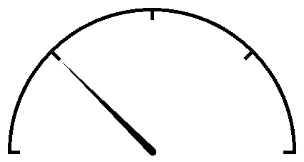
Figure 4: An analog dial and needle

Given a set $\mathcal{S}=\{R_{1},\dots,R_{n}\}$ of labeled realizations of the same degree sequence having the same vertex set $V$, define a dial with respect to $\mathcal{S}$ to be a pair of sets $(W,P)$ satisfying the following conditions.

1. The second entry $P$ is the set of all pairs of vertices from $V$ that differ in their status (adjacent or non-adjacent) among $R_{1},\dots,R_{n}$. More precisely, for $a,b\in V$, the pair $\{a,b\}$ will belong to $P$ if $ab$ is an edge in some $R_{i}$ and not an edge in some $R_{j}$, where $i,j\in\{1,\dots,n\}$. The set $W$ is the union of all pairs in $P$, so $W\subseteq V$.

2. There exist two vertices $u,v\in W$ such that for every vertex $w\in W\setminus\{u,v\}$, both the pairs $\{u,w\}$ and $\{v,w\}$ belong to $P$, and no other pair belongs to $P$.

3. In every realization $R_{i}$ for $i\in\{1,\dots,n\}$, vertex $u$ is adjacent to exactly one vertex, denoted $w_{i}$, in $W\setminus\{u,v\}$. (This edge $uw_{i}$ is called the needle in $R_{i}$.) In the same realization $R_{i}$, the vertex $v$ is not adjacent to $w_{i}$ but is adjacent to every vertex in $W\setminus\{u,v,w_{i}\}$.

Given a dial with respect to $\mathcal{S}$, the induced subgraph in any $R_{i}$ having vertex set $W$ is called a dial state. Within each $R_{i}$, the vertex set $W$ and the edges and non-edges from $P$ form a dial configuration. Ignoring vertex labels, let $\mathcal{D}_{n}$ denote an unlabeled configuration of $n+2$ vertices, $n$ edges, and $n$ non-edges arranged as in a dial configuration. With this notation, the configuration in Figure 3 is hence denoted $\mathcal{D}_{3}$.

In Figure 5 we illustrate the dial configurations in four graphs $R_{1},R_{2},R_{3},R_{4}$, using dotted segments to indicate non-adjacencies; each is an instance of $\mathcal{D}_{4}$. In each configuration the top vertex is $v$, the bottom vertex is $u$, and the middle vertices are $w_{1},w_{2},w_{3},w_{4}$. We emphasize that $u$, $v$, and the interior vertices in each configuration are the same vertices in each realization; the only thing that varies in each configuration (or in each dial state) is which pair in $P$ containing $u$ is the needle.

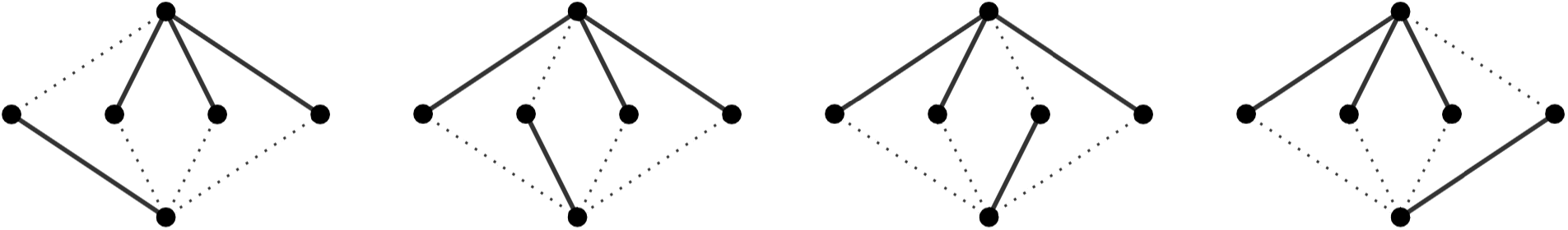
Figure 5: Configurations from states of a dial in four realizations of a degree sequence

Lemma 2.1.

If a dial exists for a set $\{R_{1},\dots,R_{n}\}$ of realizations of a degree sequence $d$, then these realizations form a clique in the realization graph $\mathcal{G}(d)$.

Furthermore, if some realization $R$ of a degree sequence $d$ contains the configuration $\mathcal{D}_{n}$, then $R$ belongs to a clique of size $n$ in $\mathcal{G}(d)$.

Proof.

Given the dial for $\{R_{1},\dots,R_{n}\}$ as indicated, let $u$, $v$, and $w_{1},\dots,w_{n}$ denote the vertices of the dial as described above. For any $i,j$ in $\{1,\dots,n\}$, the 2-switch on graph $R_{i}$ using alternating 4-cycle $[u,w_{i}:v,w_{j}]$ produces the graph $R_{j}$. Hence these realizations are pairwise adjacent in $\mathcal{G}(d)$.

Suppose now that some realization $R$ of a degree sequence $d$ contains the configuration $\mathcal{D}_{n}$. The $n-1$ alternating 4-cycles that use edges and non-edges from this configuration and include “the needle” permit 2-switches yielding $n-1$ additional, distinct realizations of $d$. It is straightforward to see that the $n+2$ vertices involved form the vertex set of a dial for these realizations, so as before $R$ belongs to a clique of size $n$ in $\mathcal{G}(d)$. ∎

In [6], Földes and Hammer characterized matrogenic graphs as those for which no five vertices’ adjacency relationships admitted the configuration $\mathcal{D}_{3}$ from Figure 3. As an immediate corollary to Lemma 2.1, we conclude that every non-matrogenic graph is a vertex in a triangle in the realization graph of its degree sequence. (With some additional conditions, the reverse implication is true; for details, see [3].)

3 Necessity of the construction

In this section we prove a near converse to Lemma 2.1.

Theorem 3.1.

If $R_{1},\dots,R_{n}$ are the vertices of a clique in a realization graph $\mathcal{G}(d)$, where $n\geq 4$, then a dial exists for this collection of graphs. Moreover, the corresponding dial configuration in each realization $R_{i}$ contains all alternating 4-cycles necessary for 2-switches converting $R_{i}$ into $R_{j}$ for $j\in\{1,\dots,n\}\setminus\{i\}$.

Observe that if $n=2$ in the hypothesis above, then the conclusion is still valid and follows from the definition of $\mathcal{G}(d)$; the states of the dial are simply the “before” and “after” versions of the alternating 4-cycle on which the 2-switch is performed. The conclusion in Theorem 3.1 does not hold for $n=3$, however; for instance, the three realizations of $(1,1,1,1)$ form a triangle in the realization graph though none contains the configuration $\mathcal{D}_{3}$. A similar result is true for many graphs containing an an induced subgraph with degree sequence $(1,1,1,1)$ or a chordless cycle on 4 vertices (in which case the graph’s complement contains the induced subgraph). Note that these examples are mentioned along with $\mathcal{D}_{3}$ in Theorem 1.1.

We prove Theorem 3.1 for the cases $n\geq 4$ by induction. Section 3.1 contains the result for $n=4$, and Section 3.2 contains the induction step.

3.1 Base case

Let $R_{1},R_{2},R_{3},R_{4}$ be the vertices of a clique of size 4 in some realization graph $\mathcal{G}(d)$. Let $m$ be the number of edges in each realization. Since these four graphs are a clique in $\mathcal{G}(d)$, for each pair $i,j$ of distinct elements in $\{1,2,3,4\}$, the graph $R_{i}$ can be transformed into $R_{j}$ by a single 2-switch. This requires that $R_{i}$ and $R_{j}$ share $m-2$ edges and that each contain two edges that the other does not.

To analyze these requirements, we let $s_{I}$ denote the number of edges that appear in every realization $R_{i}$ for $i$ displayed in the subscript $I$ and that do not appear in any realization $R_{j}$ for $j$ not displayed in $I$. Here the subscripts $I$ correspond to subsets of $\{1,2,3,4\}$ (written without enclosing braces or commas). Using a Venn diagram whose ellipses respectively represent the edge sets of $R_{1},R_{2},R_{3},R_{4}$, the variables $s_{I}$ in the interior regions of Figure 6 indicate the sizes of the subsets to which the various regions correspond.

Figure 6: Venn diagram of the edges sets of $R_{1},R_{2},R_{3},R_{4}$, with cardinalities indicated

We use these variables to describe the overlaps in our four pairwise-adjacent realizations, obtaining the following system of equations.

$$\sum_{I\ni i}s_{I} =m\qquad\text{for $1\leq i\leq 4$;}$$ (1)

$$\sum_{\begin{subarray}{c}J\ni i\\ J\not\ni j\end{subarray}}s_{J} =2\qquad\text{for $1\leq i<j\leq 4$.}$$ (2)

Here (1) holds because $R_{i}$ has exactly $m$ edges. The equations in (2) model the fact that $R_{i}$ has exactly two edges that $R_{j}$ does not, as mentioned above; as we will see shortly, the condition $i<j$ ensures that the overall system satisfies no linear dependence relations.

Using these equations, we construct a 10-by-16 augmented matrix $M$ for the system, which we display below followed by its reduced echelon form $M^{\prime}$. Here the first 15 matrix columns are indexed by the subscripts on the corresponding variables $s_{I}$, with the variables $s_{i}$ first, ordered lexicographically, followed by the variables $s_{ij}$, ordered lexicographically, followed by the variables $s_{ijk}$, in reverse lexicographic order, and followed finally by the variable $s_{1234}$.

$$M=\setcounter{MaxMatrixCols}{16}\begin{bmatrix}1&0&0&0&1&1&1&0&0&0&0&1&1&1&1&m\\ 0&1&0&0&1&0&0&1&1&0&1&0&1&1&1&m\\ 0&0&1&0&0&1&0&1&0&1&1&1&0&1&1&m\\ 0&0&0&1&0&0&1&0&1&1&1&1&1&0&1&m\\ 1&0&0&0&0&1&1&0&0&0&0&1&0&0&0&2\\ 1&0&0&0&1&0&1&0&0&0&0&0&1&0&0&2\\ 1&0&0&0&1&1&0&0&0&0&0&0&0&1&0&2\\ 0&1&0&0&1&0&0&0&1&0&0&0&1&0&0&2\\ 0&1&0&0&1&0&0&1&0&0&0&0&0&1&0&2\\ 0&0&1&0&0&1&0&1&0&0&0&0&0&1&0&2\end{bmatrix};$$

$$M^{\prime}=\setcounter{MaxMatrixCols}{16}\begin{bmatrix}1&0&0&0&0&0&0&0&0&0&0&-1&-1&-1&-2&6-2m\\ 0&1&0&0&0&0&0&0&0&0&-1&0&-1&-1&-2&6-2m\\ 0&0&1&0&0&0&0&0&0&0&-1&-1&0&-1&-2&6-2m\\ 0&0&0&1&0&0&0&0&0&0&-1&-1&-1&0&-2&6-2m\\ 0&0&0&0&1&0&0&0&0&0&0&0&1&1&1&m-2\\ 0&0&0&0&0&1&0&0&0&0&0&1&0&1&1&m-2\\ 0&0&0&0&0&0&1&0&0&0&0&1&1&0&1&m-2\\ 0&0&0&0&0&0&0&1&0&0&1&0&0&1&1&m-2\\ 0&0&0&0&0&0&0&0&1&0&1&0&1&0&1&m-2\\ 0&0&0&0&0&0&0&0&0&1&1&1&0&0&1&m-2\end{bmatrix}.$$

Having constrained the values of the variables $s_{I}$ by the system in (1) and (2), we may further restrict the possible values for these variables with a few lemmas.

Lemma 3.2.

If $I\subset\{1,2,3,4\}$ with $I\neq\emptyset$ and $I\neq\{1,2,3,4\}$, then $s_{I}\leq 1$.

Proof.

Suppose to the contrary that $s_{I}\geq 2$ for some $I$ as described.

Consider the case $|I|=1$ first. Re-indexing if necessary, we may assume that $I=\{1\}$. Taking $i=1$ and $j=2$ in (2) above, we have $s_{I}\leq 2$. However, if $s_{I}=2$, then three distinct alternating 4-cycles (those used in 2-switches changing $R_{1}$ to each of $R_{2}$, $R_{3}$, and $R_{4}$) would use the same pair of edges, which is impossible. Thus $s_{I}\leq 1$ if $|I|=1$.

We may apply this same argument to the complementary realizations $\overline{R_{1}}$, $\overline{R_{2}}$, $\overline{R_{3}}$, and $\overline{R_{4}}$, which form a clique in the realization graph of their collective degree sequence. Any edge appears in exactly one of these realizations $\overline{R_{i}}$ if and only if it is an edge in each graph $R_{j}$ for $j\in\{1,2,3,4\}\setminus\{i\}$. It follows that $s_{I}\leq 1$ if $|I|=3$ as well.

Supposing now that $|I|=2$, by re-indexing if necessary we may assume that $I=\{1,2\}$ and that $s_{12}\geq 2$. As before, (2) yields $s_{12}\leq 2$, so $s_{12}=2$. Let $uv,wx$ be these two edges in $R_{1}$. Since $R_{3}$ and $R_{4}$ have distinct edge sets, the 2-switches changing $R_{1}$ into each must differ on which non-edges are involved in the corresponding alternating 4-cycles (since both contain $uv,wx$). Without loss of generality we may assume that the 2-switch changing $R_{1}$ into $R_{3}$ uses edges non-edges $ux,vw$, and that the 2-switch changing $R_{1}$ into $R_{4}$ uses non-edges $uw,vx$. This requires that the subgraph of $R_{1}$ induced by $\{u,v,w,x\}$ be isomorphic to $2K_{2}$; the subgraph of $R_{3}$ on these vertices must be as well. Note that the edges $uv,wx$ are present in $R_{2}$ but not in $R_{3}$, so the alternating 4-cycle used in the 2-switch transforming $R_{3}$ into $R_{2}$ must include non-edges $uv,wx$ from $R_{3}$. However, the only edges in $R_{3}$ induced by the vertex set $\{u,v,w,x\}$ are the edges $ux,vw$, and if we use these edges together with the requisite non-edges in a 2-switch, instead of creating $R_{2}$ we in effect undo the previous 2-switch, recreating $R_{1}$, a contradiction.

Hence $s_{I}\leq 1$ for all sets $I\subseteq\{1,2,3,4\}$ satisfying $1\leq|I|\leq 3$. ∎

From the reduced augmented matrix $M^{\prime}$ we see that solutions to the system in (1) and (2) are determined by the value of five of the variables $s_{I}$. Lemma 3.2 implies that each variables $s_{I}$, other than $s_{1234}$, equals either 0 or 1. There are 32 solutions of the system produced by substituting candidate values for $s_{234},s_{134},s_{124},s_{123}$, and $s_{4}$; in only ten is every variable a nonnegative integer (and equal to 0 or 1 if the variable is not $s_{1234}$). We display these here, with one solution per line:

$s_{1}$	$s_{2}$	$s_{3}$	$s_{4}$	$s_{12}$	$s_{13}$	$s_{14}$	$s_{23}$	$s_{24}$	$s_{34}$	$s_{234}$	$s_{134}$	$s_{124}$	$s_{123}$	$s_{1234}$
0	0	0	0	1	1	1	1	1	1	0	0	0	0	$m-3$
0	1	1	1	1	1	1	0	0	0	1	0	0	0	$m-3$
1	0	1	1	1	0	0	1	1	0	0	1	0	0	$m-3$
1	1	0	1	0	1	0	1	0	1	0	0	1	0	$m-3$
1	1	1	0	0	0	1	0	1	1	0	0	0	1	$m-3$
1	0	0	0	0	0	0	1	1	1	0	1	1	1	$m-4$
0	1	0	0	0	1	1	0	0	1	1	0	1	1	$m-4$
0	0	1	0	1	0	1	0	1	0	1	1	0	1	$m-4$
0	0	0	1	1	1	0	1	0	0	1	1	1	0	$m-4$
1	1	1	1	0	0	0	0	0	0	1	1	1	1	$m-4$

(In the table we have used horizontal lines to group solutions that are equivalent up to permuting the names of the realizations $R_{1},R_{2},R_{3},R_{4}$.)

Though Lemma 3.2 considerably narrowed the possibilities for our candidate values for the variables $s_{I}$, even among the ten settings we have found, not all of them actually reflect a possible situation for the realizations $R_{1},R_{2},R_{3},R_{4}$. Our next lemma will rule out all possibilities but one.

Lemma 3.3.

Suppose that $A=\{i,j\}$ and $B=\{i,k\}$ for distinct elements $i,j,k$ from $\{1,2,3,4\}$. Then $s_{A}+s_{B}\leq 1$.

Proof.

Suppose to the contrary that $s_{A}+s_{B}>1$ for some sets $A,B$ as described; by Lemma 3.2 this implies that $s_{A}=s_{B}=1$. By re-indexing the realizations as necessary, we may suppose that $A=\{1,2\}$ and $B=\{1,3\}$.

Now $R_{1}$ and $R_{2}$ have an edge $e_{12}$ that does not appear in $R_{3}$ or $R_{4}$. Likewise, $R_{1}$ and $R_{3}$ have an edge $e_{13}$ that does not appear in $R_{2}$ or $R_{4}$; hence $e_{13}$ is distinct from $e_{12}$. The 2-switch transforming $R_{1}$ to $R_{4}$ must remove both edges $e_{12}$ and $e_{13}$; since these edges must appear in the corresponding alternating 4-cycle in $R_{1}$, $e_{12}$ and $e_{13}$ have no vertex in common.

However, consider the 2-switch transforming $R_{2}$ into $R_{3}$. The corresponding alternating 4-cycle in $R_{2}$ must include the edge $e_{12}$ and the non-edge $e_{13}$. This requires that $e_{12}$ and $e_{13}$ share a vertex, which we showed above is not true. The contradiction shows that for any sets $A$ and $B$ satisfying the conditions in this lemma, we have $s_{A}+s_{B}\leq 1$. ∎

Observe that in each of the first nine rows of the table above we find indices $i,j,k$ such that $s_{ij}=s_{ik}=1$, contradicting Lemma 3.3. Hence the last row must describe the edges of $R_{1},R_{2},R_{3},R_{4}$; we have $s_{i}=1$, $s_{ij}=0$, and $s_{ijk}=1$ for all distinct $i,j,k\in\{1,2,3,4\}$.

Since $s_{i}=1$ for all $i$ and $s_{I}=1$ where $I$ consists of the three elements in $\{1,2,3,4\}\setminus\{i\}$, each realization $R_{i}$ has exactly one edge $e_{i}$ that none of the other three realizations has, and exactly one non-edge $f_{i}$ that all of the other three realizations have. Think now of the 2-switches transforming $R_{1}$ into each of $R_{2},R_{3},R_{4}$. Each of these 2-switches must toggle both the edge $e_{1}$ and the non-edge $f_{1}$. It follows that $e_{1}$ and $f_{1}$ share a vertex, and taking the union of the vertex sets, edge sets, and non-edge sets of the alternating 4-cycle configurations involved in these three 2-switches results in a configuration $\mathcal{D}_{4}$ in $R_{1}$, since no two of the alternating 4-cycles can agree on the fourth vertex while still being distinct from each other. (In fact, the configuration’s respective appearances in $R_{1},R_{2},R_{3},R_{4}$ are the same as those illustrated in Figure 5.) The six vertices involved are the vertices of a dial with respect to $\{R_{1},R_{2},R_{3},R_{4}\}$ (here the edge $f_{i}$ is the needle in $R_{i}$, for each $i$), and we have established the base case in our inductive proof of Theorem 3.1.

3.2 Induction step

Suppose that the conclusion in Theorem 3.1 holds for cliques of size $k$ in every realization graph, for some $k\geq 4$. In this section we complete the induction by proving that every clique of size $k+1$ in any realization graph corresponds to the existence of a dial with respect to the realizations in the clique.

Let $\mathcal{G}(d)$ be an arbitrary realization graph having a clique of size $k+1$, and let $R_{1},\dots,R_{k+1}$ be the vertices of the clique. Applying the induction hypothesis to $R_{1},\dots,R_{k}$, we let $u,v,w_{1},\dots,w_{k}$ be the vertices of the dial $(W,P)$ for these graphs, assuming that $uw_{i}$ is the needle in $R_{i}$ for each $i\in\{1,\dots,k\}$.

If we apply the induction hypothesis to $R_{2},\dots,R_{k+1}$, we arrive at a dial $(W^{\prime},P^{\prime})$ for these graphs as well. From the first dial we note that only $u$ and $v$ appear in each of the alternating 4-cycles used for 2-switches among $R_{2},R_{3},R_{4}$. Since these alternating 4-cycles must appear in the appropriate states of the second dial, the vertices $u$ and $v$ fulfill the same roles in the second dial that they do in the first: $u$ is the vertex common to every needle edge in the second dial’s states, and $v$ is the other vertex common to every alternating 4-cycle used for 2-switches among $\{R_{2},\dots,R_{k+1}\}$. Similarly, the edges $uw_{2},\dots,uw_{k}$ are the needles for the graphs $R_{2},\dots,R_{k}$ in the second dial as well as the first. Hence the symmetric difference of $P$ and $P^{\prime}$ is

$$\{\{u,w_{1}\},\{v,w_{1}\},\{u,w_{k+1}\},\{v,w_{k+1}\}\},$$

where $w_{k+1}$ is the unique vertex in $W^{\prime}\setminus W$; note that we may assume that $w_{k+1}\neq w_{1}$, since otherwise $R_{1}=R_{k+1}$, a contradiction.

From the first dial we see that in each of $R_{2},\dots,R_{k}$, vertex $w_{1}$ is adjacent to $v$ and not to $u$. The 2-switch changing $R_{2}$ to $R_{k+1}$ does not change the neighbors of $w_{1}$, so $vw_{1}$ is an edge and $uw_{1}$ is a non-edge in $R_{k+1}$. A similar argument about the vertex $w_{k+1}$ shows that the pair $(W\cup W^{\prime},P\cup P^{\prime})$ is a dial for $R_{1},\dots,R_{k+1}$, and our proof of Theorem 3.1 is complete.

4 Conclusion

Combining Lemma 2.1 and Theorem 3.1, we have shown the following.

Theorem 4.1.

Let $d$ be a degree sequence, and let $R$ be a realization of $d$; also let $n\geq 4$. In the realization graph $\mathcal{G}(d)$ the vertex $R$ belongs to a clique of size $n$ if and only if $R$ contains the configuration $\mathcal{D}_{n}$.

Furthermore, moving in $\mathcal{G}(d)$ from $R$ to another vertex of the clique corresponds precisely to performing a 2-switch using edges and non-edges of the configuration $\mathcal{D}_{n}$ in $R$.

In Section 1 we described the seeming potential difficulty in having several labeled realizations be pairwise adjacent in a realization graph. It is perhaps not surprising that Theorem 4.1 shows that this can happen in only one way.

In this section we conclude our results by characterizing the degree sequences $d$ for which $\mathcal{G}(d)$ is a complete graph. It will turn out that there is only “one way” in which this can happen as well; however, this claim is subject to our observation in Section 1 that complementary degree sequences have the same realization graphs, and to certain addition operations we must first describe.

To keep our description mostly self-contained, we briefly recall some results from [3]. Recall that a split graph is a graph whose vertex set may be partitioned into a clique and an independent set. For any split graph, we write the degree sequence as a “splitted” sequence $(p_{2};p_{1})$, where $p_{1}$ and $p_{2}$ are respectively the sublists containing degrees of vertices in the independent set and clique. (In our notation $p_{2}$ appears before $p_{1}$ because the vertices in the clique have degrees at least as large as those in the independent set; we will assume that the sublists $p_{2}$ and $p_{1}$ are each written in nonincreasing order.)

Tyshkevich [13] defined a composition of degree sequences in the following way. If $|\pi|$ denotes the length of a list $\pi$ of integers, then for a splitted degree sequence $p=(p_{2};p_{1})$ and an arbitrary degree sequence $q$, the composition $p\circ q$ is formed by concatenating the following:

• the terms of $p_{2}$, each augmented by $|q|$,

• the terms of $q$, each augmented by $|p_{2}|$, and

• the terms of $p_{1}$.

Observe that the resulting terms of $p\circ q$ appear in descending order. Note also that if $P$ and $Q$ are respectively realizations of the degree sequences $p$ and $q$, where the vertex set of $P$ is partitioned into an independent set $V_{1}$ and a clique $V_{2}$ in such a way that the vertices in $V_{1}$ and $V_{2}$ have degrees listed in $p_{1}$ and $p_{2}$, respectively, then $p\circ q$ is the degree sequence of the graph formed by taking the disjoint union of $P$ and $Q$ and adding an edge from each vertex of $Q$ to each vertex in $V_{2}$. We denote this graph by $(P,V_{1},V_{2})\circ Q$.

If the degree sequence $q$ in the discussion above is the degree sequence of a split graph, and in the realization $Q$ the vertex set has a partition $W_{1},W_{2}$ into an independent set and clique, then $(P,V_{1},V_{2})\circ Q$ is a spit graph, and $p\circ q$ may be treated as a splitted sequence $(r_{2};r_{1})$ with the terms of $r_{1},r_{2}$ corresponding to degrees of vertices in $V_{1}\cup W_{1}$ and in $V_{2}\cup W_{2}$, respectively. With this understanding, the operation $\circ$ is associative for both degree sequences and graphs.

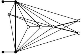
Figure 7: An example of the composition operation $\circ$

In Figure 7 we illustrate the graph $(G_{2},A_{2},B_{2})\circ(G_{1},A_{1},B_{1})\circ G_{0}$, where the graphs $G_{0},G_{1},G_{2}$ are realizations of the degree sequences $(0)$, $(3,2;1,1,1)$, and $(2,2;1,1)$, respectively. Here the vertices of $G_{0}$, $G_{1}$, and $G_{2}$ are respectively colored gray, white, and black. The sets $A_{1},A_{2}$ are comprised of the vertices of degree $1$ in $G_{1},G_{2}$, respectively, and the sets $B_{1},B_{2}$ respectively contain the other vertices of $G_{1},G_{2}$. Observe that the graph has degree sequence $(8,8,6,5,4,3,3,3,1,1)$, which equals $(2,2;1,1)\circ(3,2;1,1,1)\circ(0)$.

A degree sequence $d$ is decomposable if $d=p\circ q$ for a splitted degree sequence $p$ and a degree sequence $q$, each of length at least 1. Otherwise, $d$ is said to be indecomposable. In [13] and earlier papers referred to therein, Tyshkevich showed the following.

Theorem 4.2 ([13]).

Every degree sequence $d$ may be expressed as a composition

$$d=\alpha_{1}\circ\dots\circ\alpha_{k}\circ d_{0}$$ (3)

of indecomposable degree sequences, where each sequence $\alpha_{i}$ is a splitted degree sequence $(\beta_{i};\gamma_{i})$, and $d_{0}$. Moreover, this decomposition is unique.

We refer to such an expression (3) as the Tyshkevich decomposition of $d$.

The Tyshkevich decomposition gives us some understanding of the realization graph $\mathcal{G}(d)$. Let $G\mathbin{\text{\scalebox{0.84}{$\square$}}}H$ denote the Cartesian product of arbitrary graphs $G$ and $H$.

Theorem 4.3 ([3]).

If $d$ is a degree sequence having

$$d=\alpha_{1}\circ\dots\circ\alpha_{k}\circ d_{0}$$

as its Tyshkevich decomposition, then

$$\mathcal{G}(d)=\mathcal{G}(\alpha_{1})\mathbin{\text{\scalebox{0.84}{$\square$}}}\cdots\mathbin{\text{\scalebox{0.84}{$\square$}}}\mathcal{G}(\alpha_{k})\mathbin{\text{\scalebox{0.84}{$\square$}}}\mathcal{G}(d_{0}).$$

Since a Cartesian product $G\mathbin{\text{\scalebox{0.84}{$\square$}}}H$ can be a complete graph if and only if one of $G,H$ is a complete graph and the other has a single vertex, it follows from Theorem 4.3 that if $\mathcal{G}(d)$ is a complete graph, then all but possibly one of $\alpha_{1},\dots,\alpha_{k},d_{0}$ must have a single labeled realization.

Degree sequences having a unique labeled realization are known as threshold sequences, and their realizations are threshold graphs. (See [9] for a book-length survey on properties of these graphs.) It is known that a degree sequence $d$ is a threshold sequence if and only if in the Tyshkevich decomposition of $d$, each indecomposable sequence has a single term. In this case each indecomposable sequence has the form (0) or (0;) or (;0). (See [2] for details.)

It follows that if $\mathcal{G}(d)$ is a complete graph, then we may write $d=t\circ\alpha\circ t^{\prime}$, where both $t,t^{\prime}$ are either empty (i.e., omitted) or threshold sequences, and $\alpha$ is an indecomposable degree sequence for which $\mathcal{G}(\alpha)$ is a complete graph. We now characterize such sequences $\alpha$.

Suppose that $\alpha$ is a degree sequence for which $\mathcal{G}(\alpha)$ is isomorphic to $K_{n}$, and let $R_{1},\dots,R_{n}$ be the labeled realizations of $\alpha$. Since these realizations belongs to a clique of size $n$, Theorem 3.1 implies that a dial exists for these graphs. Adopting the same notation as in Section 2, we let $u$ (respectively, $v$) be the vertex belonging to $n-1$ non-edges (respectively, $n-1$ edges) in each dial configuration; we let $w_{1},\dots,w_{n}$ be the other dial vertices, labeled so that $uw_{i}$ is an edge in $R_{i}$ for each $i\in\{1,\dots,n\}$.

We claim that the graphs $R_{i}$ have no vertex other than those in $\{u,v,w_{1},\dots,w_{n}\}$. Note that the alternating 4-cycles formed by the edges and non-edges of a dial configuration in any realization $R_{i}$ are sufficient to provide the 2-switches transforming $R_{i}$ into every other realization among $R_{1},\dots,R_{n}$. Suppose now that $x$ is a vertex of $R_{i}$ not in $\{u,v,w_{1},\dots,w_{n}\}$. Since the degree sequence $\alpha$ is indecomposable, it is known (see [2, Lemma 3.5]) that $x$ belongs to an alternating 4-cycle. However, a 2-switch performed in $R_{i}$ on an alternating 4-cycle using $x$ would result in a realization of $\alpha$ not equal to any of $R_{1},\dots,R_{n}$, contradicting the assumption that $\mathcal{G}(\alpha)$ has just these $n$ vertices.

The need to prevent other “unauthorized” 2-switches gives us further restrictions. Fix $j\in\{1,\dots,n\}$. Suppose first that $u$ and $v$ are adjacent in $R_{j}$, and $i$ is an element of $\{1,\dots,n\}$ other than $j$. Note that if $w_{i}$ is adjacent to $w_{j}$ in $R_{j}$, then $[u,v:w_{i},w_{j}]$ is an alternating 4-cycle in $R_{j}$, and performing the associated 2-switch in $R_{j}$ results in a realization in which $w_{j}$ is adjacent to both $u$ and $v$. This is a contradiction, since $R_{1},\dots,R_{n}$ are the only realizations of $\alpha$. Hence for no $i\in\{1,\dots,n\}$ is $w_{i}$ adjacent to $w_{j}$. Moreover, since no 2-switch using edges and non-edges of the dial configuration changes the adjacency relationships among vertices in $\{w_{1},\dots,w_{n}\}$, by varying $j$ in the argument above we conclude that $\{w_{1},\dots,w_{n}\}$ must be an independent set. At this point the edges of each realization have been completely determined, and we verify that $\alpha$ is the degree sequence $\left(n,2,1^{(n)}\right)$.

A similar argument shows that if $u$ and $v$ are not adjacent in $R_{j}$, then the vertices $w_{1},\dots,w_{n}$ must be pairwise adjacent if $\mathcal{G}(d)$ is isomorphic to $K_{n}$. Here again the edges of $R_{j}$ and all other realizations have been completely determined; in this case $\alpha$ is the degree sequence $\left(n^{(n)},n-1,1\right)$.

A straightforward verification shows that both $\left(n,2,1^{(n)}\right)$ and $\left(n^{(n)},n-1,1\right)$ have exactly $n$ realizations, each of which is isomorphic to the appropriate graph shown in Figure 8, and the degree sequences have $K_{n}$ as their realization graph.

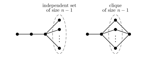
Figure 8: Graphs whose realization graphs are complete graphs

The discussion above proves our final result.

Theorem 4.4.

For any $n\geq 4$ and any degree sequence $d$, the realization graph $\mathcal{G}(d)$ is a complete graph of order $n$ if and only if $d=t\circ\alpha\circ t^{\prime}$, where each of $t,t^{\prime}$ is either empty (i.e., omitted) or a threshold sequence, and $\alpha$ is $\left(n,2,1^{(n)}\right)$ or $\left(n^{(n)},n-1,1\right)$.

References

- [1] S.R. Arikati, U.N. Peled, The realization graph of a degree sequence with majorization gap 1 is Hamiltonian, Linear Algebra Appl. 290 (1–3) (1999), 213–235.
- [2] M.D. Barrus and D.B. West, The -structure of a graph, J. Graph Theory 71 (2012), no. 2, 159–175.
- [3] M.D. Barrus, On realization graphs of degree sequences, Discrete Mathematics 339 (2016), no. 8, 2146–2152.
- [4] R.A. Brualdi, Matrices of zeros and ones with fixed row and column sum vectors, Linear Algebra Appl. 33 (1980), 159–231.
- [5] R.B. Eggleton and D.A. Holton, Graphic sequences, Combinatorial Mathematics VI, Proc. 6th Australian Conference, Lecture Notes in Mathematics 748, Springer-Verlag, New York, 1979, pp. 1–10.
- [6] S. Földes, P.L. Hammer, On a class of matroid-producing graphs, in: A. Hajnal, V.T. Sós (Eds.), Combinatorics, Kesthely (Hungary), in: Colloquia Mathematica Societatis János Bolyai, vol. 18, North-Holland, Budapest, 1978, pp. 331–352.
- [7] D.R. Fulkerson, A.J. Hoffman, and M.H. McAndrew, Some properties of graphs with multiple edges, Canad. J. Math. 17 (1965) 166–177.
- [8] S.L. Hakimi, On realizability of a set of integers as degrees of the vertices of a linear graph. II. Uniqueness, J. Soc. Indust. Appl. Math. 11 (1963), 135–147.
- [9] N.V.R. Mahadev and U.N. Peled, Threshold graphs and related topics. Annals of Discrete Mathematics, 56. North-Holland Publishing Co., Amsterdam, 1995.
- [10] N. Nishimura, Introduction to reconfiguration, Algorithms (Basel) 11 (2018), no. 4, Paper No. 52.
- [11] J. Petersen, Die Theorie der regulären Graphen, Acta Math. 15 (1891), 193–220.
- [12] J.K. Senior, Partitions and their representative graphs, Amer. J. Math. 73 (1951), 663–689.
- [13] R. Tyshkevich, Decomposition of graphical sequences and unigraphs, Discrete Mathematics 220 (2000), 201–238.