Quasi-Framelets: Another Improvement to Graph Neural Networks

Abstract

This paper aims to provide a novel design of a multiscale framelets convolution for spectral graph neural networks. In the spectral paradigm, spectral GNNs improve graph learning task performance via proposing various spectral filters in spectral domain to capture both global and local graph struture information. Although the existing spectral approaches show superior performance in some graphs, they suffer from lack of flexibility and being fragile when graph information are incomplete or perturbated. Our new framelets convolution incorporates the filtering functions directly designed in the spectral domain to overcome these limitations. The proposed convolution shows a great flexibility in cutting-off spectral information and effectively mitigate the negative effect of noisy graph signals. Besides, to exploit the heterogeneity in real-world graph data, the heterogeneous graph neural network with our new framelet convolution provides a solution for embedding the intrinsic topological information of meta-path with a multi-level graph analysis. Extensive experiments have been conducted on real-world heterogeneous graphs and homogeneous graphs under settings with noisy node features and superior performance results are achieved.

1 Introduction

The recent decade has witnessed graph neural networks (GNNs), as a deep representation learning method for graph data, have aroused considerable research interests. Duvenaud et al. [7] and Kipf & Welling [14] delivered the GCN (Graph Convolution Networks) with significantly improved performance on the semi-supervised node classification tasks, since then a large number of GNN variants have been proposed, including GAT [25], GraphSAGE [9], GIN [29], and DGI [26].

The empirical successes of GNNs in both node-level and graph-level tasks have prompted the need of well understanding in a systematic and theoretical way. For example, PPNP and APPNP [15] try to establish a connection between the graph convolution operator of GCN and the Graph-regularized graph signal processing. The graph-regularized layer has been recently exploited to signal denoising, node and edge attack [33]. However, researchers have also found that one of pitfalls of GNNs is its performance degradation due to oversmoothing with deep layers [20]. Hong and Maehara [19] shew that GNNs only perform low-pass filtering on original node feature vectors.

The two main streams of designing GNNs are the graph spatial view (such as message passing see [14]) and the graph spectral view (such as via graph Laplacian spectral decomposition) [4]. Under the graph spectral view, one makes use of graph convolutions known from spectral graph theory. The graph signals are mapped into the graph spectral domain under the Fourier framework, then appropriate filters either pre-defined or learned are applied on the signals, and finally filtered spectral signals will be either reconstructed back to the spatial or piped straightaway to the next networks for further processing.

In the spectral paradigm, different spectral GNNs differs in the way how to regulate signals through spectral filters in spectral domain. All these can be clustered as two major approaches: (1) The learning approach and (2) The approach of applying mathematically designed filters. For example, under the first approach, Defferrard et al. [4] utilize K-order Chebyshev polynomials to approximate smooth filters in the spectral domain. Kipf and Welling [13] propose a spectral approach where a graph convolutional network is designed via a localized first-order approximation of spectral graph convolutions. Under the second approach, for example, Li et al. [16] introduce Haar basis to solve high computational cost of eigen-decompositions of graph Laplacian which allows scalability of graphs. The concept of wavelet frames has been developed for a long time [18] and shows a wide range of applications like signal processing and filter bank design. The wavelet transformation has been constructed on graphs based on defining scaling using the spectral decomposition of the discrete graph Laplacian [11] and applied in image processing [22].

In applications, understanding graphs from a multiscale or multiresolution perspective is critical in acquiring structure of graph networks. Ying et al. [30] proposed a multiresolution graph neural network to build a hierarchical graph representation. For the purpose of multiresolution graph signal representation and analysis, by combining tight wavelet frames and spectral graph theory, Dong [5] develops tight graph framelets and shows an efficient and accurate representation of graphs. In this approach, the built-in mathematical tight framelets are applied on the spectral domain of graph Laplacian to achieve the filtering purpose. As demonstrated in [32], the framelets can take care of regulating low-pass and high-pass information from graph signals simultaneously to achieve better than state-of-the-art performance.

Both the learning approach and the mathematically designed approach have been successful in many graph learning tasks. However there are couple of explicit limitation in terms of graph signal filtering. The learning approach leaves the filtering capability entirely to the end-to-end learning from data. In some sense this may be too sensitive to data change. While applying those mathematically built-in wavelets or framelets to filtering in spectral domain in the second approach, the power of filters have been fixed due to the mathematical design. This is not flexible in the case when one wishes to clearly cut off certain spectral information. This paper will propose a way in between the above approaches by directly designing filtering functions in the spectral domain. While the new method still has learning capacity through filter learning, thus it does offer the flexibility in cutting-off specific spectral information.

All the aforementioned approaches focus on homogeneous graphs where nodes and edges are of the same types respectively. As a matter of fact, the real-world graphs, such as social networks and academic networks, show nodes and edges of multiple types. In order to capture the heterogeneity of these graphs, heterogeneous graph neural networks have been introduced and some research have been explored for mining the information hidden in these heterogeneous graphs. Heterogeneous graphs can characterize complex graphs and contain rich semantics. Most existing heterogeneous GNN models, such as HAN [27], HGT [12] and HGCN [34] extend message-passing graph neural network framework to perform spatial-based graph convolutions on heterogeneous graphs. Through projecting features of various types of nodes onto a common feature space, these heterogeneous GNN models implement message passing directly from spatially close neighbors. Further, measuring the spatially closeness takes semantic information, which are defined by meta-paths or meta-graphs, into consideration.

However, the spectral-based methods have been far behind explored on heterogenous graphs. One of typical ways to deal with heterogeneous graphs (as done in literature) is to convert a heterogeneous graph into several homogeneous subgraphs. For example, consider the academic network with authors (A), papers (P), venues (V), organizations (O) as nodes. The meta-path “APA” representing the coauthor relationships on a paper (P) between two authors (A) defines a homogeneous subgraph, and similarly the meta-path “APVPA” representing two authors (A) publishing papers (P) in the same venue (V) defines another homogeneous subgraph. Then one simply applies the classic GNNs like GCNs on such subgraphs. This construction can suffer from the fact that a cohort of high frequency Laplacian eigenvectors may contain meaningful information jointly, i.e., multiresolution structures. However the current approaches used in embedding heterogeneous graphs may not be able to access this information. As the homogeneous subgraphs comes from several chosen meta-path types and those relevant graph Laplacian may carry multiresolution structure information. A naïve application of message passing may ingore such mutliresolition pattern. In fact, a framelet-assisted GNN will benefit incorporating such mutliresolution pattern for heterogeneous graphs. This is one of major motivations we explore the application of framelet transformation on heterogeneous graphs.

In summary, our contributions in this paper are in five-fold:

1. To our best knowledge, this is the first attempt to introduce frametlet-based convolutions on heterogeneous graph neural network. The proposed framelet convolution leverages framelet transforms to decompose graph data into low-pass and high-pass spectra in a fine-tuned multiscale way, which shows superior performance in preserving node feature information and graph geometric information and to achieve a fast decomposition and reconstruction algorithm.

2. We propose a new way of designing multiscale framelets from spectral perspective. The new way offers both learning capacity and flexibility in e.g. cutting-off unwanted spectral information. The experiments demonstrate the state-of-the-art performance.

3. We demonstrate that the framelet construction no longer rely on the multiple finite filter banks in the spatial domain. This leaves the room for designing any specific framelets as appropriate for meaningful frequency suppression.

4. We theoretically prove that the new system has all the theoretical properties of the classic framelets such as the fast algorithm in decomposition and reconstruction.

5. The results of extensive experiments prove the effectiveness of node representation learnt by our model and show the superiority of the model prediction performance against state-of-the-art methods.

2 Preliminaries

This section serves a quick summary on the classic spectral graph neural networks and the basic terms used in heterogeneous graphs for our purposes in the sequel.

2.1 Classic Spectral Graph Neural Networks

Two main streams in constructing a GNN (graph neural networks) layer are the spatial perspective [13, 25] and the spectral perspective [1, 4, 28]. Here we are concerned with the spectral view which is related to our proposed quasi-framelet method. We provide a brief introduction.

First, we consider homogeneous graphs. Specifically we denote $\mathcal{G}=(\mathcal{V},\mathcal{E})$ as an undirected (homogeneous) graph, where $\mathcal{V}=\{v_{n}\}^{N}_{n=1}$ is the set of $N$ nodes, and $\mathcal{E}=\{e_{ij}=(v_{i},v_{j})\}$ is the set of edges with cardinality $E=|\mathcal{E}|$. The adjacency matrix is denoted by $\mathbf{A}\in\mathbb{R}^{N\times N}$ such that $A_{ij}=1$ if $e_{i,j}=(v_{i},v_{j})$ is an edge of the graph.

The classic Vanilla spectral GNN layer [13] is defined based on the orthogonal spectral bases $\mathbf{U}=\{u_{1},...,u_{N}\}$ extracted from the graph Laplacian where each base $u_{i}\in\mathbb{R}^{N}$ can be regarded as a graph signal defined on each node. For example, one usually takes $\mathbf{U}$ as the matrix of eigenvectors of the normalized graph Laplacian $\mathbf{L}=\mathbf{I}_{N}-\mathbf{D}^{-1/2}\mathbf{A}\mathbf{D}^{-1/2}=\mathbf{U}\boldsymbol{\Lambda}\mathbf{U}$, with a diagonal matrix of all the eigenvalues (spectra) $\boldsymbol{\Lambda}=\{\lambda_{1},...,\lambda_{N}\}$ of $\mathbf{L}$. For any graph signal $\mathbf{x}$, its graph spectral transformation is defined as

$$g_{\theta}\star\mathbf{x}=\mathbf{U}g_{\theta}(\boldsymbol{\Lambda})\mathbf{U}^{T}\mathbf{x}$$ (1)

where $g_{\theta}(\boldsymbol{\Lambda})=\text{diag}(g_{\theta}(\lambda_{1}),...,g_{\theta}(\lambda_{N}))$ with the full set of spectra related to the spectral bases. Here $g_{\theta}$ is a designated spectral modulation function which can be learnable and sometimes $\mathbf{U}^{T}\mathbf{x}$ is called the graph Fourier transform of graph signal $\mathbf{x}$.

In [14], for the purpose of a fast algorithm, the modulation function $g_{\theta}(\cdot)$ is approximated by Chebyshev polynomial approximation, thus the Chebyshev coefficients in the approximation can be made learnable. This is to say one chooses $g_{\theta}(\cdot)$ to be a polynomial. The classic spatial GCN is a special case when one uses the first order Chebyshev approximation. When putting $g_{\theta}(\cdot)$ in an end-to-end learning fashion, one loses control over the modulator’s capacity in controlling specific spectral components.

Authors of [3] take advantage of the fact that the spectral transformation (1) only relies on $N$ modulation function values at the spectra $\boldsymbol{\Lambda}$, i.e., over $\{\lambda_{1},...,\lambda_{N}\}$, reparameterize these function values straightaway for learning, and split their parameters into higher frequency group and lower frequency group, then merge them in the transformation. However it is not clear what the best strategy in splitting is.

Framelet analysis is a successful mathematical signal process approach, even for signals defined on manifolds [5]. This idea has been recently applied for graph signals [32]. Instead of using a single modulation function $g_{\theta}$, a group of modulation functions in spectral domain were used, i.e., the scaling functions in Framelet terms. Based on the Multiresolution Analysis (MRA), those scaling functions $\Psi=\{\alpha;\beta^{(1)},...,\beta^{(K)}\}$ are constructed from a set of (finite) filter bank $\eta=\{a;b^{(1)},...,b^{(K)}\}\subset l_{0}(\mathbb{Z})$. In Fourier frequency domain, such scaling functions can jointly regulate the spectral frequency by applying them on the spectra $\boldsymbol{\Lambda}$ as done in (1) with the ability of multiscaling, raised from the following relations of framelets

$$\widehat{\alpha}(2\xi)=\widehat{a}(\xi)\widehat{\alpha}(\xi),\widehat{\beta^{(k)}}(2\xi)=\widehat{b^{(k)}}(\xi)\widehat{\alpha}(\xi)$$ (2)

for $k=1,2,...,K$. One of drawback from this forward framelet strategy is it is unclear what high frequency can be removed and what low frequency can be kept.

2.2 Heterogeneous Graphs

For a self-explained paper, in this section, the basic definitions of heterogeneous graphs, meta-paths used for heterogeneous graphs as well as relative concepts are reviewed.

Definition 1 (Heterogeneous graphs).

A heterogeneous graph is defined as a directed graph HG = $(\mathcal{V},\mathcal{E},\mathcal{S},\mathcal{R})$ where each node $v$ and each edge $e$ are associated with their type mapping function $\tau(\upsilon)$: $V\rightarrow\mathcal{S}$ and $\phi(e):E\rightarrow\mathcal{R}$, respectively.

Definition 2 (Meta path).

A meta-path $\Phi$ is defined as a path in the form of $S_{1}\xrightarrow{R_{1}}S_{2}\xrightarrow{R_{2}}...\xrightarrow{R_{l}}S_{l}$, which describes a composite relation $R=R_{1}\circ R_{2}\circ...\circ R_{l}$ between objects $S_{1}$ and $S_{l+1}$, where $\circ$ denotes the composition operator on relations.

Clearly a meta-path $\Phi$ defines a relation $R$ between two nodes $v$ and $u$ of types $S_{1}$ and $S_{L}$. In this case, we call $u$ is a meta-path $\Phi$ neighbor of node $v$. Also we say that there is a relation $R$ between node $v$ and $u$. Denote by $N_{v}^{\Phi}$ the set of all such neighbors of a node $v$.

Definition 3 (Meta-path based graph and adjacency matrix).

Given a meta-path $\Phi$ whose starting vertices are of type $S_{1}$ and ending vertices are of type $S_{l}$, the meta-path based graph $\mathcal{G}^{\Phi}$ is a graph constructed from all node pairs $v\in S_{1}$ and $u\in S_{l}$ that connect via meta-path $P$. A meta-path based adjacency matrix $A^{\Phi}$ can be constructed.

Meta-path based graphs can exploit different aspects of structure information in heterogeneous graph. Majority of heterogeneous graph embeddings can be categorized into random walk-based and neural network-based methods. However, both of these methods mainly consider meta-paths or meta-graphs to incorporate heterogeneous structural information. For example, metapath2vec [6] designs a meta-path based random walk and utilizes skip-gram to perform heterogeneous graph embedding. The random walk-based model only considers metapath-based semantic information but loses enough information about graph structures. Meanwhile, this type of “shallow” models is limited to be applied for transductive tasks which means they cannot deal with nodes that do not appear in the training process.

On the other hand, Meta-path Aggregated Graph Neural Network (MAGNN) [8] defines meta-path-based neighbor nodes and propagates feature and structural information along meta-paths to generate the embedding of the target type node. Heterogeneous attention networks [27] consider attention of nodes and semantics and learn node embeddings from meta-path-based neighbors. Similar to MAGNN [8], HAN [27] adopts the message passing framework to apply a spatial-based graph convolution for node representation learning, while this paper focus on spectral-based methods. Besides, Heterogeneous graph neural networks [31] set up a unified framework to jointly introduce heterogeneity in node feature information and graph structures, without considering the semantics in heterogeneous graphs.

Heterogeneous graphs are a type of information network, containing either multiple types of objects or multiple types of relations. In heterogeneous graphs, objects can be connected via edges of various types. The employment of meta-paths can capture the relation types between two node types. Besides, based on meta-paths, a heterogeneous graph can be broken into a set of per-meta-path subgraphs and further, be represented as a set of meta-path-based adjacency matrices. In this paper, we are only concerned with the meta-path based graphs in which the two ending nodes of the meta-path are in a same given type $S$ (i.e. $S_{1}=S_{L}=S$). This type of meta-aoth based graph is indeed a homogeneous graph in which all the nodes are in the unique type and edges (paths) are in the same type too. In a number of applications represented in such as HAN [27], HGT [12] and HGCN [34], the heterogeneous graph neural networks are built on their homogeneous meta-path based subgraphs. In our experiments, when we adopt the framelet analysis for heterogeneous graphs, we break down the heterogeneous graphs into such homogeneous subgraphs and learns filters based on framelet domain to multiscale structure information hidden in a heterogeneous graph.

3 The Model based on Quasi-Framelets

In this section, we consider homogeneous graph and perform quasi-framelets on the graph. A new Quasi-Framelet transform functions and a fast algorithm for the transformation are instroduced in this part.

3.1 The Quasi-Framelet Transform

Our idea will follow the basic Framelet theory, however we will work backwards. Rather than looking for scaling functions from the finite filter banks in spatial domain, we aim to directly construct the spectral modulation functions in the spectral domain. The starting point is from the necessary conditions for signal decomposition (Fourier transform) and reconstruction (Inverse Fourier transform).

Definition 4 (Modulation functions for Quasi-Framelets).

We call a set of $K+1$ positive modulation functions defined on $[0,\pi]$, $\mathcal{F}=\{g_{0}(\xi),g_{1}(\xi),...,g_{K}(\xi)\}$, a quasi-framelet if it satisfies the following identity condition

$$g_{0}(\xi)^{2}+g_{1}(\xi)^{2}+\cdots+g_{K}(\xi)^{2}\equiv 1,\;\;\;\forall\xi\in[0,\pi]$$ (3)

such that $g_{0}$ decreases from 1 to 0 and $g_{K}$ increases from 0 to 1 over the spectral domain $[0,\pi]$.

Particularly $g_{0}$ aims to regulate the high frequency while $g_{K}$ to regulate the lower frequency, and the rest to regulate other frequency between.

Here we propose two sets of such modulation functions, some of which are shown in Figure 1:

1. Sigmoid Modulation Functions ($K=1$):

   $$g_{0}(\xi) =\sqrt{1-\frac{1}{1+\exp\{-\alpha(\xi/\pi-0.5)\}}}$$

   $$g_{1}(\xi) =\sqrt{\frac{1}{1+\exp\{-\alpha(\xi/\pi-0.5)\}}}$$

   where $\alpha>0$. In our experiment we take $\alpha=20$ to ensure sufficient modulation power at both lowest and highest frequency.

2. Entropy Modulation Functions ($K=2$):

   $$g_{0}(\xi) =\begin{cases}\sqrt{1-g^{2}_{1}(\xi)},&\xi<=\pi/2\\ 0,&\text{otherwise}\end{cases}$$

   $$g_{1}(\xi) =\sqrt{4\alpha\xi/\pi-4\alpha\left(\xi/\pi\right)^{2}}$$

   $$g_{2}(\xi) =\begin{cases}\sqrt{1-g^{2}_{1}(\xi)},&\xi>\pi/2\\ 0,&\text{otherwise}\end{cases}$$

   where $0<\alpha\leq 1$ could be a learnable parameter. In our experiment, we empirically set $\alpha=0.75$. When $\alpha=1$, $g^{2}_{1}(\pi\xi)$ is the so-called binary entropy function.

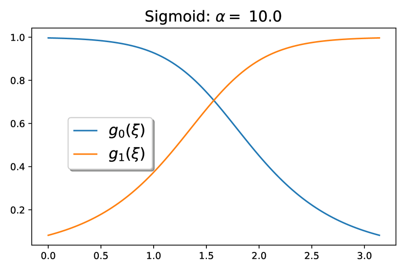
(a) Sigmoid modulation Functions ($\alpha=10$)

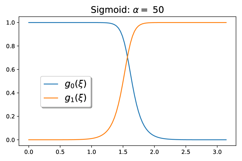
(b) Entropy modulation Functions ($\alpha=50$)

(c) Entropy modulation Functions ($\alpha=0.5$)

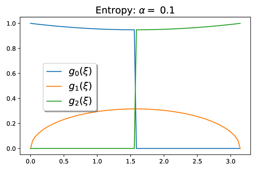
(d) Entropy modulation Functions ($\alpha=0.1$)

Figure 1: (a) and (b): examples of sigmoid modulation fucntions with (learnable) parameter $\alpha=10$ and with $\alpha=50$, respectively; (c) and (d): examples of entropy modulation functions with (learnable) parameter $\alpha=0.5$ and with $\alpha=0.1$, respectively.

Now consider an undirected (homogeneous) graph $\mathcal{G}=(\mathcal{V},\mathcal{E})$ and any graph signal $\mathbf{x}$ defined on its nodes. Suppose that $\mathbf{U}$ is the orthogonal spectral bases given by the normalized graph Laplacian $\mathbf{L}$ with its spectra $0\leq\lambda_{1}\leq\lambda_{2}\leq\cdots\leq\lambda_{N}$. To build an appropriate spectral transformation defined as (1), for a given set of quasi-framelet functions $\mathcal{F}=\{g_{0}(\xi),g_{1}(\xi),...,g_{K}(\xi)\}$ defined on $[0,\pi]$ and a given level $L$ ($\geq 0$), define the following quasi-framelet signal decomposition

$$\widehat{\mathbf{x}}=\mathcal{W}\mathbf{x}.$$ (4)

where the matrix operator $\mathcal{W}=[\mathcal{W}_{0,L};\mathcal{W}_{1,0};...;\mathcal{W}_{K,0};\mathcal{W}_{1,1};...,\mathcal{W}_{K,L}]$ is stacked from the following the signal transformation matrices

$$\mathcal{W}_{0,L} =\mathbf{U}g_{0}(\frac{\boldsymbol{\Lambda}}{2^{L+m}})\cdots g_{0}(\frac{\boldsymbol{\Lambda}}{2^{m}})\mathbf{U}^{T},$$ (5)

$$\mathcal{W}_{k,0} =\mathbf{U}g_{k}(\frac{\boldsymbol{\Lambda}}{2^{m}})\mathbf{U}^{T},\text{for }k=1,...,K,$$ (6)

$$\mathcal{W}_{k,l} =\mathbf{U}g_{k}(\frac{\boldsymbol{\Lambda}}{2^{m+l}})g_{0}(\frac{\boldsymbol{\Lambda}}{2^{m+l-1}})\cdots g_{0}(\frac{\boldsymbol{\Lambda}}{2^{m}})\mathbf{U}^{T},\text{for }k=1,...,K,l=1,...,L.$$ (7)

Note that in the above definition, $m$ is called the coarsest scale level which is the smallest $m$ satisfying $2^{-m}\lambda_{N}\leq\pi$. Then the quasi-framelet reconstruction can be implemented as

Theorem 1.

The quasi-framelet decomposition (4) admits a perfect reconstruction given by

$$\mathbf{x}=\mathcal{W}^{T}\widehat{\mathbf{x}}.$$ (8)

i.e. $\mathcal{W}^{T}\mathcal{W}=\mathbf{I}_{N}$.

Proof.

According to the definition of all signal transformation matrices, all $\mathcal{W}_{i,j}$ are symmetric. Hence we have

$$\mathcal{W}^{T}\mathcal{W}=\mathcal{W}^{T}_{0,L}\mathcal{W}_{0,L}+\sum^{L}_{l=0}\sum^{K}_{k=1}\mathcal{W}^{T}_{k,l}\mathcal{W}_{k,l}$$

$$= \mathcal{W}_{0,L}\mathcal{W}_{0,L}+\sum^{K}_{k=1}\mathcal{W}_{k,L}\mathcal{W}_{k,L}+\sum^{L-1}_{l=}\sum^{K}_{k=1}\mathcal{W}_{k,l}\mathcal{W}_{k,l}$$

$$= \mathbf{U}g^{2}_{0}(\frac{\boldsymbol{\Lambda}}{2^{L+m}})\cdots g^{2}_{0}(\frac{\boldsymbol{\Lambda}}{2^{m}})\mathbf{U}^{T}+\sum^{K}_{k=1}\mathbf{U}g^{2}_{k}(\frac{\boldsymbol{\Lambda}}{2^{m+L}})g^{2}_{0}(\frac{\boldsymbol{\Lambda}}{2^{m+L-1}})\cdots g^{2}_{0}(\frac{\boldsymbol{\Lambda}}{2^{m}})\mathbf{U}^{T}+\sum^{L-1}_{l=}\sum^{K}_{k=1}\mathcal{W}_{k,l}\mathcal{W}_{k,l}$$

$$= \mathbf{U}\left(g^{2}_{0}(\frac{\boldsymbol{\Lambda}}{2^{L+m}})+\sum^{K}_{k=1}g^{2}_{k}(\frac{\boldsymbol{\Lambda}}{2^{m+L}})\right)g^{2}_{0}(\frac{\boldsymbol{\Lambda}}{2^{m+L-1}})\cdots g^{2}_{0}(\frac{\boldsymbol{\Lambda}}{2^{m}})\mathbf{U}^{T}+\sum^{L-1}_{l=}\sum^{K}_{k=1}\mathcal{W}_{k,l}\mathcal{W}_{k,l}$$

$$= \mathbf{U}g^{2}_{0}(\frac{\boldsymbol{\Lambda}}{2^{m+L-1}})\cdots g^{2}_{0}(\frac{\boldsymbol{\Lambda}}{2^{m}})\mathbf{U}^{T}+\sum^{L-1}_{l=0}\sum^{K}_{k=1}\mathcal{W}_{k,l}\mathcal{W}_{k,l}$$

$$\vdots$$

$$= \mathbf{U}g^{2}_{0}(\frac{\boldsymbol{\Lambda}}{2^{m}})\mathbf{U}^{T}+\sum^{K}_{k=1}\mathbf{U}g^{2}_{k}(\frac{\boldsymbol{\Lambda}}{2^{m}})\mathbf{U}^{T}=\mathbf{U}(g^{2}_{0}(\frac{\boldsymbol{\Lambda}}{2^{m}})+\sum^{K}_{k=1}g^{2}_{k}(\frac{\boldsymbol{\Lambda}}{2^{m}}))\mathbf{U}^{T}=\mathbf{U}\mathbf{U}^{T}=\mathbf{I}_{N}.$$

where we have repeatedly used the condition (3). This completes the proof. ∎

3.2 Graph Quasi-Framelets

The quasi-framelet signal decomposition (4) gives the signal decomposition coefficient. To better understand how the signal was decomposed on the framelet bases, we can define the following graph quasi-framelets as follows which can be regarded the signals in the spatial space.

Suppose $\{(\lambda_{i},\mathbf{u}_{i})\}^{N}_{i=1}$ are the eigenvalue and eigenvector pairs for the noramlized Laplacian $\mathbf{L}$ of graph $\mathcal{G}$ with $N$ nodes. The quasi-framelets at scale level $\ell=1,...,L$ for graph $\mathcal{G}$ with a given set of modulation functions $\mathcal{F}=\{g_{0}(\xi),g_{1}(\xi),...,g_{K}(\xi)\}$ are defined, for $k=1,...,K$, by

$$\phi_{\ell,p}(v) =\sum^{N}_{i=1}g_{0}(\frac{\lambda_{i}}{2^{\ell}})\mathbf{u}_{i}(p)\mathbf{u}_{i}(v)$$ (9)

$$\psi^{k}_{\ell,p}(v) =\sum^{N}_{i=1}g_{k}(\frac{\lambda_{i}}{2^{\ell}})\mathbf{u}_{i}(p)\mathbf{u}_{i}(v)$$ (10)

for all nodes $u,p$ and $\phi_{\ell,p}$ or $\psi^{k}_{\ell,p}$ is the low-pass or high-pass framelet translated at node $p$, see [5].

It is clear that the low-pass and high-pass framelet coefficients for a signal $\mathbf{x}$ on graph $\mathcal{G}$ are $v_{\ell,p}$ and $w^{k}_{\ell,p}$, which are the projections $\langle\phi_{\ell,p},\mathbf{x}\rangle$ and $\langle\psi^{k}_{\ell,p},\mathbf{x}\rangle$ of the graph signal onto framelets at scale $\ell$ and node $p$.

Similar to the standard undecimated framelet system [5], we can define the quasi-framelet system BUFS as follows. For any two integers $L,L_{1}$ satisfying $L>L_{1}$, we define an quasi-framelet system $\text{BUFS}(\mathcal{F};\mathcal{G})$ (starting from a scale $J_{1}$) as a non-homogeneous, stationary affine system:

$$\text{BUFS}^{L}_{L_{1}}(\mathcal{F};\mathcal{G}):=\{\phi_{L_{1},p}:p\in\mathcal{V}\}\cup\{\psi^{k}_{\ell,p}:p\in\mathcal{V},\ell=L_{1},...,L\}^{K}_{k=1}$$ (11)

The system $\text{BUFS}^{L}_{L_{1}}(\mathcal{F};\mathcal{G})$ is then called a quasi-tight frame for graph signal space $L^{2}(\mathcal{G})$ and the elements in $\text{BUFS}^{L}_{L_{1}}(\mathcal{F};\mathcal{G})$ are called quasi tight framelets on $\mathcal{G}$, quasi-framelets for short.

All the theory about the quasi-framelet can be guaranteed in the following theorem.

Theorem 2 (Equivalence of Quasi-Framelet Tightness).

Let $\mathcal{G}=(\mathcal{V},\mathcal{E})$ be a graph and $\{(\lambda_{i},\mathbf{u}_{i})\}^{N}_{i=1}$ be the eigenvalue and eigenvector pairs for its noramlized Laplacian $\mathbf{L}$. Let $\mathcal{F}=\{g_{0}(\xi),g_{1}(\xi),...,g_{K}(\xi)\}$ be a set of quasi-framelet functions satisfying the identity condition (3). For $L>L_{1}$, $\text{BUFS}^{L}_{L_{1}}(\mathcal{F};\mathcal{G})$ is the quasi-framelet system given in (11). Then the following statements are equivalent.

1. For each $L_{1}=1,...,L$, the quasi-framelet system $\text{BUFS}^{L}_{L_{1}}(\mathcal{F};\mathcal{G})$ is a tight frame for $L^{2}(\mathcal{G})$, that is, $\forall\mathbf{x}\in L^{2}(\mathcal{G})$,

   $$\|\mathbf{x}\|^{2}=\sum_{p\in\mathcal{V}}|\langle\phi_{L_{1},p},\mathbf{x}\rangle|^{2}+\sum^{L}_{\ell=L_{1}}\sum^{K}_{k=1}\sum_{p\in\mathcal{V}}|\langle\psi^{k}_{\ell,p},\mathbf{x}\rangle|^{2}.$$

2. For all $\mathbf{x}\in L^{2}(\mathcal{G})$ and for $\ell=1,...,L-1$, the following identities hold

   $$\mathbf{x} =\sum_{p\in\mathcal{V}}\langle\phi_{L,p},\mathbf{x}\rangle\phi_{L,p}+\sum^{K}_{k=1}\sum_{p\in\mathcal{V}}\langle\psi^{k}_{L,p},\mathbf{x}\rangle\psi_{L,p}$$

   $$\sum_{p\in\mathcal{V}}\langle\phi_{\ell+1,p},\mathbf{x}\rangle\phi_{\ell+1,p} =\sum_{p\in\mathcal{V}}\langle\phi_{\ell,p},\mathbf{x}\rangle\phi_{\ell,p}+\sum^{K}_{k=1}\sum_{p\in\mathcal{V}}\langle\psi^{k}_{\ell,p},\mathbf{x}\rangle\psi_{\ell,p}$$

3. For all $\mathbf{x}\in L^{2}(\mathcal{G})$ and for $\ell=1,...,L-1$, the following identities hold

   $$\|\mathbf{x}\|^{2}=\sum_{p\in\mathcal{V}}|\langle\phi_{L,p},\mathbf{x}\rangle|^{2}+\sum^{K}_{k=1}\sum_{p\in\mathcal{V}}|\langle\psi^{k}_{L,p},\mathbf{x}\rangle|^{2}.$$

   $$\sum_{p\in\mathcal{V}}|\langle\phi_{\ell+1,p},\mathbf{x}\rangle|^{2}=\sum_{p\in\mathcal{V}}|\langle\phi_{\ell,p},\mathbf{x}\rangle|^{2}+\sum^{K}_{k=1}\sum_{p\in\mathcal{V}}|\langle\psi^{k}_{\ell,p},\mathbf{x}\rangle|^{2}$$

Proof.

A proof can be given by strictly following the proof of Theorem 1 in [32]. ∎

3.3 Fast Algorithm for the Quasi-Framelet Transform

Both the quasi-framelet signal decomposition and reconstruction (4) and (8) are the building-block for our quasi-framelet convolution. However in its current form, it is computationally prohibitive for a large graph, as it will cost $O(N^{3})$ to get the eigendecomposition of the Laplacian.

Similar to the standard spectral GNNs, we will adopt a polynomial approximation to each modulation function $g_{j}(\xi)$ ($j=0,1,...,K$). We approximate $g_{j}(\xi)$ by Chebyshev polynomials $\mathcal{T}^{n}_{j}(\xi)$ of a fixed degree $n$ where the integer $n$ is chosen such that the Chebyshev polynomial approximation is of high precision. In practice, $n=3$ is good enough. For simple notation, in the sequel, we use $\mathcal{T}_{j}(\xi)$ instead of $\mathcal{T}^{n}_{j}(\xi)$. Then the quasi-framelet transformation matrices defined in (5) - (7) can be approximated by

$$\mathcal{W}_{0,L} \approx\mathbf{U}\mathcal{T}_{0}(\frac{\boldsymbol{\Lambda}}{2^{L+m}})\cdots\mathcal{T}_{0}(\frac{\boldsymbol{\Lambda}}{2^{m}})\mathbf{U}^{T}=\mathcal{T}_{0}(\frac{1}{2^{L+m}}{\mathbf{L}})\cdots\mathcal{T}_{0}(\frac{1}{2^{m}}{\mathbf{L}}),$$ (12)

$$\mathcal{W}_{k,0} \approx\mathbf{U}\mathcal{T}_{k}(\frac{\boldsymbol{\Lambda}}{2^{m}})\mathbf{U}^{T}=\mathcal{T}_{k}(\frac{1}{2^{m}}\mathbf{L}),\;\;\;\text{for }k=1,...,K,$$ (13)

$$\mathcal{W}_{k,l} \approx\mathbf{U}\mathcal{T}_{k}(\frac{\boldsymbol{\Lambda}}{2^{m+l}})\mathcal{T}_{0}(\frac{\boldsymbol{\Lambda}}{2^{m+l-1}})\cdots\mathcal{T}_{0}(\frac{\boldsymbol{\Lambda}}{2^{m}})\mathbf{U}^{T}$$

$$=\mathcal{T}_{k}(\frac{1}{2^{m+l}}\mathbf{L})\mathcal{T}_{0}(\frac{1}{2^{m+l-1}}\mathbf{L})\cdots\mathcal{T}_{0}(\frac{1}{2^{m}}\mathbf{L}),\text{for }k=1,...,K,l=1,...,L.$$ (14)

As an example, we use heatmap in Figure 2 show these approximation matrices.

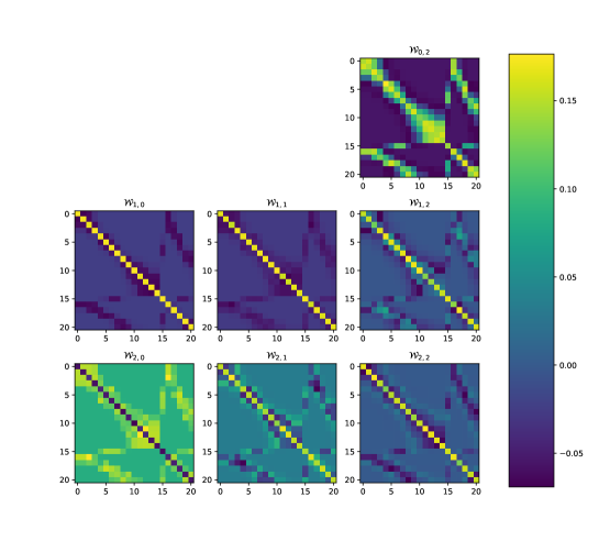
Figure 2: Quasi-framelet transformation matrices $\mathcal{W}_{k,l}$ at different scales from the left column $l=0$ to the right column $l=L=2$, for a graph with 21 nodes. The first row corresponds to the lowest frequency for the entropy modulation function $g_{0}(\xi)$, the middle row $g_{1}(\xi)$, and the third row $g_{2}(\xi)$, based on (12)-(14).

Hence the quasi-framelet transformation matrices are approximated by calculating the matrix power of the normalized Laplacian $\mathbf{L}$. Thus for a graph signal $\mathbf{x}$, its framelet $\text{BUFS}^{L}_{1}(\mathcal{F},;\mathcal{G})$ (see (11)) can be approximated calculated by the following iteration, which also gives the graph signal quasi-framelet decomposition (4),

Start with:

$$\Phi_{0,0}:=\mathcal{T}_{0}(\frac{1}{2^{m}}\mathbf{L})\mathbf{x};$$

$$\Psi_{k,0}:=\mathcal{T}_{k}(\frac{1}{2^{m}}\mathbf{L})\mathbf{x};\text{for }k=1,...,K$$

for $$\ell=1,...,L,\text{do: }$$

$$\Phi_{0,\ell}:=\mathcal{T}_{0}(\frac{1}{2^{\ell+m}}\mathbf{L})\Phi_{0,\ell-1};$$

$$\Psi_{k,\ell}:=\mathcal{T}_{k}(\frac{1}{2^{\ell+m}}\mathbf{L})\Phi_{0,\ell-1};\text{for }k=1,...,K$$

Similarly for any given quasi-framelet signal $\widehat{\mathbf{x}}$, represented by its framelet $\text{BUFS}^{L}_{1}(\mathcal{F},;\mathcal{G})$ i.e., in vector form $\{\Phi_{0,L}\}\cup\{\Psi_{k,\ell}\}^{K,L}_{k=1,\ell=1}$, the reconstruction (8) can be implemented in the following recursive algorithm:

for $$\ell=L,...,1,\text{do:}$$

$$\Phi_{0,\ell-1}:=\mathcal{T}_{0}(\frac{1}{2^{\ell+m}}\mathbf{L})\Phi_{0,\ell}+\sum^{K}_{k=1}\mathcal{T}_{k}(\frac{1}{2^{\ell+m}}\mathbf{L})\Psi_{k,\ell}$$

Then:

$$\mathbf{x}\approx\mathcal{T}_{0}(\frac{1}{2^{m}}\mathbf{L})\Phi_{0,0}+\sum^{K}_{k=1}\mathcal{T}_{k}(\frac{1}{2^{m}}\mathbf{L})\Psi_{k,0}.$$

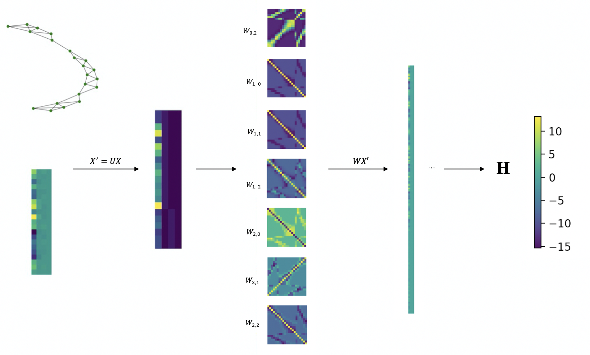
Figure 3: The framework of quasi-framelet convolution layer. The whole process is represented by a 21-node toy graph which has a 21 $\times$ 4 feature matrix. During the process, our model transforms graph signals ( transformed node features $\mathbf{X}^{\prime}$) first and apply the filter matrices $\mathcal{W}_{k,l}$ from high-pass frequency to the highest-pass frequency. Finally, graph signals will be reconstructed and node representation $\mathbf{H}$ will be obtained which will be sent to the next layer or the task-related objective.

3.4 Quasi-Framelet Convolution

Similar to classic spectral graph convolutions, we can easily define our quasi-framelet convolutions as shown in Figure 3. Suppose the input node feature $\mathbf{X}\in\mathbb{R}^{(N\times d)}$ of the graph $\mathcal{G}$, i.e., the signal is in $d$ channels. Then the graph quasi-framelet convolution can be represented as:

$$g_{\theta}\star\mathbf{X}=\sigma(\mathcal{W}^{T}g_{\theta}\circ(\mathcal{W}\mathbf{X}))$$ (15)

where the diagonal $g_{\theta}$ represents a learnable filter to be applied on the spectral coefficients of the signal and $\sigma$ is the layer activation function such as a ReLu activation. The diagonal operators further modulate the spectral coefficients from all $d$ signal channels. Moreover, using these diagonal operators reduces the number of parameters of a filter from $N\times d$ to $N$.

In the convolution $g_{\theta}\star\mathbf{X}$, the transforms $\mathcal{W}$ and $\mathcal{W}^{T}$ can be implemented by the fast decomposition and reconstruction algorithms introduced in the last subsection.

4 Experiments

Our main purpose is to demonstrate the proposed quasi-framelets (QUFG) are powerful in assisting graph learning. We will consider its comparison with the classic GCN [13], UFG [32] and GAT [25] in learning tasks for both homogeneous and heterogeneous graphs.

In this section, experiments on real-world networks are conducted to demonstrate the effectiveness and efficiency of the proposed Quasi-framelets model. Besides, our work also focuses on two applications of the Quasi-framelet Transform: denoising and representation on heterogeneous graphs. Relevant experiments are performed respectively on real homogeneous networks and heterogeneous networks.

Table 1: The Statistics of Graph Datasets

Homo-Data	Nodes	Edges	Feats	#Cls	Heter-Data	Nodes	Edges	Feats	#Cls
Cora	2708	5429	1433	7	DBLP	2708	5429	334	4
Citeseer	3327	4732	3703	6	IMDB	3327	4732	1232	3
Pubmed	19717	44338	500	3	ACM	19717	44338	1830	3

4.1 Experimental Settings

4.1.1 Datasets

We give a quick description on the datasets that we will use in our experiments

Citation networks. To evaluate the effectiveness of the proposed model QUFG, we conduct experiments on four citation networks in Table 1, including Cora, Citeseer , PubMed, will be used in node classification tasks.

Heterogeneous networks. To show the capability of our model applied in heterogeneous networks, three widely used heterogeneous graph datasets are adopted to evaluate the performance of the model and the detailed descriptions of these datasets are represented on the right columns of Table 1.

DBLP: A subset of DBLP which contains 14328 papers (P), 4057 authors (A), 20 conferences (C), 8789 terms (T). There are four working areas for authors: database, data mining, machine learning, information retrieval. Author features are the elements of a bag-of-words represented of keywords. Following the setting as [27], in our experiment, we use the meta-path set {APA, APCPA, APTPA} to define three homogeneous graphs to conduct quasi-framelet analysis.

ACM: Papers published in KDD, SIGMOD, SIGCOMM, MobiCOMM and VLDB are extracted, and the papers are categorized into three types: Database, Wireless Communication, Data Mining. This dataset offer a heterogeneous graph that consists of 3025 papers (P), 5835 authors (A) and 56 subjects (S). Still the bag-of-words are used as the paper features. Two constructed homogeneous graphs are with the meta-path types {PAP, PSP} to perform experiments. Here we label the papers according to the conference they published.

IMDB: This heterogenous graph contains 4780 movies (M), 5841 actors (A) and 2269 directors (D). We consider three types of the movies: Action, Comedy, Drama. Similarly the bag-of-words features for Movies are used. Our QUFG analysis is conducted on the homogeneous graphs of the meta-path set {MAM, MDM} to perform experiments.

4.1.2 Baseline Model/Methods and Experimental Settings

To evaluate the performances on homogeneous graphs and heterogeneous graphs separately, our model is compared with several baselines. 1) spectral GNN methods: SPECTRAL CNN [2], CHEBYSHEV [4], GWNN [28], LANCZOSNET [17], UFGCONV [32]; 2) spatial GNN methods: GCN [13], GAT [25], GraphSAGE [10]; 3) Heterogeneous GNN methods: DeepWalk [21], ESim [23], Metapath2 [6], HAN[27], UFGCONV on heterogeneous graphs.

For each experiment, we report the average results of 10 runs. Except for some default hyper-parameters, hyper-parameters, such as learning rates, number of hidden units, of all models are tuned based on the result on the validation set. Through the parameter tunning, for Cora and Citeseer datasets the number of hidden units is 32, learning rate is 0.01 and the number of iterations is 200 with early stopping on the validation set. For PubMed dataset, experiments are conducted with 64 hidden units , 0.005 learning rate and 250 iterations. For experiments on heterogeneous graphs, on IMDB and ACM datasets, the number of hidden units is 16, number of layers is 3, learning rate is 0.005 and number of epochs is 200. Besides, a similar set of parameters are used on DBLP dataset except for the number of hidden units which is 64.

4.2 The Synthetic Study

We design a number of tests on the deliberately noised Cora data for the node classification task. The network consists of two layers of quasi-framelet spectral convolution as defined in (15) and the extra soft thresholding strategy was used, see [32]. For model training, we fix the number of the hidden neuron at $16$ and the dropout ratio at $0.3$ for all the models, with Adam optimizer.

4.2.1 Experiment 1: dilation levels

In the first experimental test, we aim to test the performance of GCNs (15) when using both UFG and QUFG ($\alpha=0.1$) in denoising. As the UFG has been demonstrated as the best performer in [32], we only take the UFG as the benchmark for a comparison. We test denoising two types of noises: (1) spreading $bn=15\%$, $30\%$ and $50\%$ poison with random binary noise; (2) injecting Gaussian white noise with standard deviation at levels $nl=5.0$, 10.0 and 20.0 into all the features. The filters in UFG model and QUFG model are conducted and compared by scale $s=2.5$ and scale $s=1.1$ respectively.

Table 2: Denoising Results: Cora Node Classification Accuracy

NoiseType	NoiseLevel	scale $s=1.1$		scale $s=2.5$
		QUFG	UFG	QUFG	UFG
Binary	$bn=50\%$	62.66$\pm$0.0227	60.58$\pm$0.0274	60.09$\pm$0.0285	57.26$\pm$0.0288
	$bn=30\%$	67.91$\pm$1.47	66.40$\pm$1.29	65.35$\pm$1.28	61.82$\pm$1.54
	$bn=15\%$	71.62$\pm$0.90	70.56$\pm$0.72	67.89$\pm$0.48	69.64$\pm$0.64
Gaussian	$nl=20$	56.26$\pm$1.91	54.42$\pm$1.39	54.16$\pm$1.02	51.41$\pm$1.12
	$nl=10$	59.17$\pm$1.26	57.19$\pm$1.15	55.60$\pm$1.24	52.89$\pm$1.49
	$nl=5$	63.47$\pm$1.03	62.09$\pm$0.77	59.68$\pm$1.07	57.45$\pm$1.32

The results in Table 2 show that QUFG has better capacity in denoising data. The result shows that the new QUFG outperforms UFG in almost all scenarios for both Gaussian noises and binary poisoning noises.

4.2.2 Experiment 2: high frequency noise

In the second experimental test, we aim to demonstrate the capacity of the proposed QUFG in denoising relevant graph high frequency components against the state-of-the-art UFG framelets.

To simulate the high frequency noises, we will pick up the eigenvectors of the normalized Laplacian $\mathbf{L}$ corresponding to the larger eigenvalues. Assume that $\mathbf{L}=\mathbf{U}\boldsymbol{\Lambda}\mathbf{U}^{\top}$ where the eigenvalues $\boldsymbol{\Lambda}$ are in a decreasing order, then the noises to be injected into the node signal will be given

$$\mathbf{n}=\mathbf{U}[:,1:F]\mathbf{w}$$

where $F$ is the number of high frequency components with two choices ($F=100$ or $500$) and $\mathbf{w}$ in shape $[F,1]$ is the noise levels, randomly chosen from normal distribution with standard deviation levels $nl=5.0$, 10.0 and 20.0, respectively. We will use the benchmark parameters as [32], by setting two GCN layers, hidden feature $nhid=16$, Chebyshev order $n=3$ (we use this order for a more accurate Chebyshev approximation. In fact the results for $n=2$ demonstrate a similar pattern, see Appendix.), Soft threshold for denoising, weight decay 0.01 and learning rate 0.005 with epoch number 200.

We consider two high frequency components cut-off strategies: (a) PartialCutoff — in (15) setting $\mathcal{W}_{K,0}=0$ to remove the highest frequency; and (b) FullCutoff — in (15) setting $\mathcal{W}_{K,l}=0$ ($l=0,1,...,L$) to remove all the high frequencies.

Table 3: Denoising Results: Cora Node Classification Accuracy

NumFreq	NoiseLevel	PartialCutoff		FullCutoff
		QUFG	UFG	QUFG	UFG
$F=100$	$nl=20$	82.08$\pm$0.29	52.71$\pm$1.90	82.06$\pm$0.27	71.13$\pm$0.67
	$nl=10$	81.94$\pm$0.25	66.58$\pm$0.70	82.03$\pm$0.25	76.06$\pm$0.63
	$nl=5$	82.17$\pm$0.18	73.28$\pm$0.60	81.79$\pm$0.94	78.40$\pm$0.56
$F=500$	$nl=20$	80.43$\pm$0.78	26.81$\pm$0.70	80.45$\pm$0.50	29.05$\pm$1.47
	$nl=10$	80.68$\pm$0.63	28.45$\pm$1.05	80.95$\pm$0.63	32.78$\pm$0.90
	$nl=5$	81.50$\pm$0.82	32.13$\pm$0.64	81.62$\pm$0.83	43.54$\pm$0.97

Experimental results under both partial cutoff and full cutoff settings are demonstrated in Table 3. In both PartialCutoff and FullCutoff settings, with a group of entropy modulation functions, QUFG model demonstrates its performance of a very similar accuracy pattern in all the cases, while accuracy performance of UFG model looks significantly different for two cut-off strategies. This is because one of strengths of the Entropy framelet is its capability to fully cut off the high frequencies not matter at what noise scales, while as UFG framelet was designed from spatial domain, there is no control over what frequency components should be regulated for the UFG model. Furthermore, although UFG can denoise relevant high frequency components (in the case of $F=100$), it almost fails in identifying mild high frequencies components (in the case of $F=500$). As the entropy framelets were designed by clearly cutting off the relevant high frequency components through zero values of $g_{0}$ and $g_{2}$, the experiment results show that the entire frequency band is clearly separated by the QUFG model.

4.3 Empirical Study I: More Benchmark Comparisons On Denoising Effect

We use the QUFG graph convolution g to denoise node features X by $g_{\theta}\star\mathbf{X}$, which provides us the denoised features. On citation graph datasets, Cora and Citeseer, nodes represent documents and node features are bag-of-words representation of the documents. In details, one target node is a scientific publication described by a 0/1-valued word vector. In this node feature vector, 0 and 1 respectively indicates absence and presence of words in a dictionary which consists of 1433 unique words. For the purpose of illustrating the models’ capabilities in node feature denoising, we use binary noises and represent various noise magnitudes of nodes on a graph by different percentages of poisoned node’s features. Binary noises on node features can be seen as some words missing and some node features added in a paper. Meanwhile, node features in Pubmed dataset are described by a TF/IDF weighted word vector which is a set of float values between 0 and 1. The denoising setting for node classification tasks on Pubmed dataset will be Gaussian noises which are distributed with zero mean and various standard deviations to show the levels of noises.

Our QUFG model is designed to reduce perturbations on node features. In order to compare its superior ability with other spectral GNNs and spatial GCN baselines, node classification task is conducted and accuracy results are obtained. The experiment results show that all the spectral graph convolutions are largely affected by noises. In the denoising setting, QUFG model shows a superior performance compared with both spectral graph convolutions and spatial graph convolutions.

4.3.1 Node classification on graphs without noise.

Node classification performance of both spatial GCN, GAT and spectral GCN on semi-supervised learning for three basic graphs, Cora, CiteSeer and Pubmed has been represented in Table 4.

Table 4: Test Accuracy (%) for Citation Networks. Note: * indicates no published std available.

Method	Cora	Citeseer	Pubmed
Spectral [2]	73.3*	58.9*	73.9*
Chebyshev [4]	81.2*	69.8*	74.4*
GCN [13]	81.5*	70.3*	79.0*
GWNN [28]	82.8*	71.7*	79.1*
GAT [25]	83.0$\pm$0.7	72.5$\pm$0.7	79.0$\pm$0.3
GRAPHSAGE [10]	74.5$\pm$0.8	67.2$\pm$1.0	76.8$\pm$0.6
LANCZOSNET [17]	79.5$\pm$1.8	66.2$\pm$1.9	78.3$\pm$0.3
UFGCONV-S [32]	83.0$\pm$0.5	71.0$\pm$0.6	79.4$\pm$0.4
UFGCONV-R [32]	83.6$\pm$0.6	72.7$\pm$0.6	79.9$\pm$0.1
QUFGCONV-E (Ours)	83.9$\pm$0.79	73.4$\pm$0.62	80.6$\pm$0.78
QUFGCONV-S (Ours)	83.3$\pm$1.2	71.3$\pm$0.7	80.1$\pm$0.29

We report the accuracy scores in percentage and top one performance results have been highlighted. Besides, there are no standard deviation for test accuracies in first four results since they are not provided in their paper. Through comparisons with other models, our QUFG achieved the highest result. The QUGF-E model (with entropy modulation) outperformed the rest including QUGF-S (sigmoid modulation) on all these citation graphs since for the node level task, the model includes a learnable parameter in its modulation functions and is designed to separate true node features and noises precisely.

Meanwhile, we conduct a sensitive test on the learnable parameter alpha which is set in the learning filter. On different graphs, the optimal alphas for achieving the highest test accuracy varied. The optimal alphas are 0.78, 0.6, 0.3 for graphs Cora, CiteSeer and PubMed respectively. This indicates the high flexibility of QUFG-E convolution when graph data changes as demonstrated in Figure 4.

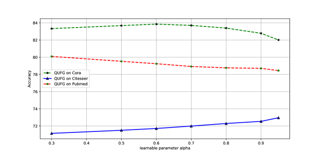
Figure 4: For datasets Cora, Citeseer and Pubmed, accuracy results of QUFG-E GNN model corresponding to various learnable parameter $\alpha$ in entropy modulation function ranging from 0.3 to 0.95.

4.3.2 Node classification on graphs with noise.

We measured the denoising capability of the QUFG-E GCN for node classification tasks by adding noises onto citation graphs. First, the denoising experiments on Cora and CiteSeer are performed by including binary noises on node features. Besides, PubMed will be employed to test the model’s capabilities in dealing with Gaussian noises.

Table 5: Accuracy (%) in Binary Noise Setting

Datasets	NoiseLevel (%)	5	15	25	50
Cora	Spectral [2]	26.03 $\pm$ 5.08	19.53 $\pm$ 4.12	15.23 $\pm$ 4.69	19.12 $\pm$ 6.89
	Chebyshev [4]	30.57 $\pm$ 4.43	30.92 $\pm$ 2.60	21.51 $\pm$ 7.59	18.07 $\pm$ 4.07
	GCN [13]	76.73 $\pm$ 0.77	67.78 $\pm$ 0.95	60.97 $\pm$ 0.85	54.46 $\pm$ 2.38
	GWNN [28]	43.46 $\pm$1.55	30.24 $\pm$ 0.90	23.57$\pm$ 1.34	20.06 $\pm$ 3.17
	UFG [32]	75.61 $\pm$ 0.81	70.56 $\pm$ 0.72	66.85 $\pm$ 1.67	60.58 $\pm$ 2.74
	QUFG (Ours)	79.1 $\pm$ 0.90	71.62 $\pm$ 1.18	68.2 $\pm$ 2.07	62.66 $\pm$ 2.05
Citeseer	Spectral [2]	18.99 $\pm$ 1.43	17.58 $\pm$ 3.87	17.97 $\pm$ 2.55	20.34 $\pm$ 4.54
	Chebyshev [4]	19.4 $\pm$ 1.81	17.29 $\pm$ 4.14	18.22 $\pm$ 2.73	17.2 $\pm$ 3.31
	GCN [13]	62.58 $\pm$ 0.84	47.30 $\pm$ 1.16	39.42 $\pm$ 1.05	31.88 $\pm$ 2.50
	GWNN [28]	49.43 $\pm$ 1.35	21.13 $\pm$ 0.26	21.28 $\pm$ 0.46	15.82 $\pm$ 06.92
	UFG [32]	61.64 $\pm$ 1.28	40.80 $\pm$ 6.96	25.97 $\pm$ 3.21	23.50 $\pm$ 2.72
	QUFG (Ours)	60.86 $\pm$ 1.76	47.38 $\pm$ 1.75	44.90 $\pm$ 2.34	42.44 $\pm$ 1.63

Table 5 reports the node classification results under the binary denoising settings: (1) binary noises with different binary noise levels which represents what percentage of nodes are poisoned by binary noises; (2) Gaussian noises with different levels represented by various standard deviations. The results show that QUFG model shows superior performance over the baseline models in most cases, which proves QUFG model’s denoising strength.

Table 6: Accuracy (%) in Gaussian Noise Setting

Dataset	NoiseLevel (%)	5	10	20
Pubmed	Spectral [2]	37.36 $\pm$ 3.50	36.68 $\pm$ 3.19	36.45 $\pm$ 3.07
	Chebyshev [4]	37.59 $\pm$ 3.30	35.69 $\pm$ 2.77	36.82 $\pm$ 2.99
	GCN [13]	44.13$\pm$ 1.40	42.59 $\pm$ 1.40	41.11 $\pm$ 2.69
	GWNN [13]	20.87$\pm$0.36	19.63$\pm$0.25	19.59 $\pm$ 0.22
	UFG [32]	43.3 $\pm$ 2.11	42.90 $\pm$ 1.48	41. 35 $\pm$ 1.87
	QUFG (Ours)	43.61 $\pm$ 2.97	43.83 $\pm$ 1.71	41.47 $\pm$ 2.24

Table 6 reports the accuracy performances of various GNN models conducting node classification tasks on Pubmed dataset under the Gaussian denoising settings. Gaussian noises are set with different levels represented by various standard deviations: 0.05, 0.1 and 0.2. The results show that QUFG model shows superior performance over the baseline models in nearly all the cases, which proves QUFG model’s denoising strength.

4.4 Empirical Study II: Applications in Heterogeneous Graph

The main purpose of this set of experiments is to show the potential of using quasi-framelet in hetereogeous embedding learning for node classification. We will use the HAN [27] as our benchmark for comparison. We are not accessing performance against some Heterogeneous GNN models like MAGNN [8] because MAGNN works in a totally different setting which conducts message passing on meta-path.

Given one input heterogeneous graph, we break the heterogeneous graph into a group of homogeneous graphs defined by meta-path based neigbourhood and construct a set of corresponding meta-path-based adjacency matrices where heterogeneity of both node types and edge types can be captured. Through applying the quasi-framelets on each meta-path, we obtain the node representations by aggregating information from meta-path based neighbors and then take a semantic information merging.

We conduct experiments on the ACM, IMDB and DBLP datasets to compare the performance of different models on the node classification task. The experiments for both UFG and QUFG GCNs are conducted based on 10 runs, with hidden unit number 32 (ACM) or 64 (the other two), scale 1.5. Other parameters setting are based on the experimental setting used in HAN [27], but the core component attention module in HAN has been simply replaced with our QUFGConv module. The other results are copied from [27] in which there is no standard deviation is available.

Table 7: Heterogeneous Graph Node Classification Accuracy (std in brackets)

Models	DBLP		ACM		IMDB
	Macro-F1	Micro-F1	Macro-F1	Micro-F1	Macro-F1	Micro-F1
DeepWalk [21]	77.43	79.37	77.25	76.92	40.72	46.38
ESim [23]	91.64	92.73	77.32	76.89	32.10	35.28
metapath2 [6]	90.16	91.53	65.09	65.00	41.16	45.65
HERcc [24]	91.68	92.69	66.17	66.03	41.65	45.81
GCN [13]	90.79	91.71	86.81	86.77	45.73	49.78
GAT [25]	90.97	91.96	86.23	86.01	49.44	55.28
HAN [27]	92.24	93.11	89.40	89.22	50.00	55.73
UFG [32]	90.55	91.78	91.45	91.42	54.96	56.75
	(1.08)	(0.97)	(0.29)	(0.28)	(1.17)	(1.57)
QUFG (ours)	91.67	92.76	92.72	92.70	55.69	58.56
	(0.64)	(0.56)	(0.38)	(0.38)	(0.76)	(1.02)

Here is a preliminary analysis over the results. It is quite interesting that almost all the models except for DeepWalk perform comparably, while HAN takes the first place, and our QUFG takes the second place for both metrics. However for both ACM and IMDB, our QUFG outperforms all the other models including its framelet family UFG (with linear framelet). It is our belief that the multiple explicit frequency component decomposition power given by QUFG does extract and regulate different frequency components hidden in the heterogeneous graphs. There is no need to use attention mechanism to extract such hidden relations.

5 Conclusion

From the spectral GCN perspective, we directly formulate filtering functions in the spectral domain. By introducitng the two sets of novel modulation functions, we define the QUFG convolution for GNNs, which shows flexibility and denoising capability in node classification task. Besides, instead of attention mechanism, QUFG convolution offers a graph representation which improves the performance of heterogeneous graph learning for node classification.

References

- [1] Muhammet Balcilar, Guillaume Renton, Pierre Héroux, Benoit Gaüzère, Sébastien Adam, and Paul Honeine. Analyzing the expressive power of graph neural networks in a spectral perspective. In International Conference on Learning Representations, 2020.
- [2] Joan Bruna, Wojciech Zaremba, Arthur Szlam, and Yann LeCun. Spectral networks and locally connected networks on graphs. arXiv preprint arXiv:1312.6203, 2013.
- [3] Heng Chang, Yu Rong, Tingyang Xu, Wenbing Huang, Somayeh Sojoudi, Junzhou Huang, and Wenwu Zhu. Spectral graph attention network with fast eigen-approximation. In KDD Workshop on Deep Learning on Graphs: Method and Applications (DLG-KDD21), 2021.
- [4] Michaël Defferrard, Xavier Bresson, and Pierre Vandergheynst. Convolutional neural networks on graphs with fast localized spectral filtering. Advances in neural information processing systems, 29:3844–3852, 2016.
- [5] Bin Dong. Sparse representation on graphs by tight wavelet frames and applications. Applied and Computational Harmonic Analysis, 42(3):452–479, 2017.
- [6] Yuxiao Dong, Nitesh V Chawla, and Ananthram Swami. metapath2vec: Scalable representation learning for heterogeneous networks. In Proceedings of the 23rd ACM SIGKDD international conference on knowledge discovery and data mining, pages 135–144, 2017.
- [7] David K Duvenaud, Dougal Maclaurin, Jorge Iparraguirre, Rafael Bombarell, Timothy Hirzel, Alan Aspuru-Guzik, and Ryan P Adams. Convolutional networks on graphs for learning molecular fingerprints. In C. Cortes, N. Lawrence, D. Lee, M. Sugiyama, and R. Garnett, editors, Advances in Neural Information Processing Systems, volume 28. Curran Associates, Inc., 2015.
- [8] Xinyu Fu, Jiani Zhang, Ziqiao Meng, and Irwin King. Magnn: Metapath aggregated graph neural network for heterogeneous graph embedding. In Proceedings of The Web Conference 2020, pages 2331–2341, 2020.
- [9] Will Hamilton, Zhitao Ying, and Jure Leskovec. Inductive representation learning on large graphs. In Advances in Neural Information Processing Systems, pages 1024–1034, 2017.
- [10] William L Hamilton, Rex Ying, and Jure Leskovec. Inductive representation learning on large graphs. In Proceedings of the 31st International Conference on Neural Information Processing Systems, pages 1025–1035, 2017.
- [11] David K. Hammond, Pierre Vandergheynst, and Rémi Gribonval. Wavelets on graphs via spectral graph theory. Applied and Computational Harmonic Analysis, 30(2):129–150, 2011.
- [12] Ziniu Hu, Yuxiao Dong, Kuansan Wang, and Yizhou Sun. Heterogeneous graph transformer. In Proceedings of The Web Conference 2020, pages 2704–2710, 2020.
- [13] Thomas N Kipf and Max Welling. Semi-supervised classification with graph convolutional networks. arXiv preprint arXiv:1609.02907, 2016.
- [14] Thomas N. Kipf and Max Welling. Semi-supervised classification with graph convolutional networks. In Proceedings of International Conference on Learning Representation, pages 1–14, 2017.
- [15] Johannes Klicpera, Aleksandar Bojchevski, and Stephan Günnemann. Predict then propagate: Graph neural networks meet personalized pageran. In Proceedings of ICLR, 2019.
- [16] Ming Li, Zheng Ma, Yu Guang Wang, and Xiaosheng Zhuang. Fast haar transforms for graph neural networks. Neural Networks, 128:188–198, 2020.
- [17] Renjie Liao, Zhizhen Zhao, Raquel Urtasun, and Richard S. Zemel. Lanczosnet: Multi-scale deep graph convolutional networks, 2019.
- [18] Stphane Mallat. A Wavelet Tour of Signal Processing, Third Edition: The Sparse Way. Academic Press, Inc., USA, 3rd edition, 2008.
- [19] Hoang NT and Takanori Maehara. Revisiting graph neural networks: All we have is low-pass filters. arXiv preprint:1905.09550, 2019.
- [20] Kenta Oono and Taiji Suzuki. Graph neural networks exponentially lose expressive power for node classification. In Porceedings of International Conference on Learning Representations (ICLR), 2020.
- [21] Bryan Perozzi, Rami Al-Rfou, and Steven Skiena. Deepwalk. Proceedings of the 20th ACM SIGKDD international conference on Knowledge discovery and data mining, Aug 2014.
- [22] Yusuf Yigit Pilavci and Nicolas Farrugia. Spectral graph wavelet transform as feature extractor for machine learning in neuroimaging. In Proceedings of IEEE International Conference on Acoustics, Speech and Signal Processing (ICASSP), pages 1140–1144, 2019.
- [23] Jingbo Shang, Meng Qu, Jialu Liu, Lance M Kaplan, Jiawei Han, and Jian Peng. Meta-path guided embedding for similarity search in large-scale heterogeneous information networks. arXiv preprint arXiv:1610.09769, 2016.
- [24] Chuan Shi, Binbin Hu, Wayne Xin Zhao, and S Yu Philip. Heterogeneous information network embedding for recommendation. IEEE Transactions on Knowledge and Data Engineering, 31(2):357–370, 2018.
- [25] Petar Veličković, Guillem Cucurull, Arantxa Casanova, Adriana Romero, Pietro Lio, and Yoshua Bengio. Graph attention networks. arXiv preprint arXiv:1710.10903, 2017.
- [26] Petar Velićković, William Fedus, William L, Hamilton, Pietro Lió, Yoshua Bengio, and R DevonHjelm. Deep graph infomax. In Proceedings of International Conference on Learning Representations (ICLR), 2019.
- [27] Xiao Wang, Houye Ji, Chuan Shi, Bai Wang, Yanfang Ye, Peng Cui, and Philip S Yu. Heterogeneous graph attention network. In The World Wide Web Conference, pages 2022–2032, 2019.
- [28] Bingbing Xu, Huawei Shen, Qi Cao, Yunqi Qiu, and Xueqi Cheng. Graph wavelet neural network. arXiv preprint arXiv:1904.07785, 2019.
- [29] Keyulu Xu, Weihua Hu, Jure Leskovec, and Stefanie Jegelka. How powerful are graph neural networks? In Proceedings of International Conference on Learning Representations (ICLR), 2019.
- [30] R. Ying, J. You, C. Morris, X. Ren, W. L. Hamilton, and J. Leskovec. Hierarchical graph representation learning with differentiable pooling. In Proceedings of the International Conference on Neural Information Processing Systems (NeuRIPS), pages 4805–4815. Curran Associates Inc., 2018.
- [31] Chuxu Zhang, Dongjin Song, Chao Huang, Ananthram Swami, and Nitesh V Chawla. Heterogeneous graph neural network. In Proceedings of the 25th ACM SIGKDD International Conference on Knowledge Discovery & Data Mining, pages 793–803, 2019.
- [32] Xuebin Zheng, Bingxin Zhou, Junbin Gao, Yuguang Wang, Pietro Lió, Ming Li, and Guido Montúfar. How framelets enhance graph neural networks. In Marina Meila and Tong Zhang, editors, Proceedings of the 38th International Conference on Machine Learning, ICML 2021, 18-24 July 2021, Virtual Event, volume 139 of Proceedings of Machine Learning Research, pages 12761–12771. PMLR, 2021.
- [33] Bingxin Zhou, Ruikun Li, Xuebin Zheng, Yu Guang Wang, and Junbin Gao. Graph denoising with framelet regularizer. arXiv: submitted to IEEE PAMI, 2021.
- [34] Zhihua Zhu, Xinxin Fan, Xiaokai Chu, and Jingping Bi. Hgcn: A heterogeneous graph convolutional network-based deep learning model toward collective classification. In Proceedings of the 26th ACM SIGKDD International Conference on Knowledge Discovery & Data Mining, pages 1161–1171, 2020.