Multiple Hypothesis Testing To Estimate The Number of Communities in Sparse Stochastic Block Models

Abstract

Network-based clustering methods frequently require the number of communities to be specified a priori. Moreover, most of the existing methods for estimating the number of communities assume the number of communities to be fixed and not scale with the network size $n$. The few methods that assume the number of communities to increase with the network size $n$ are only valid when the average degree $d$ of a network grows at least as fast as $O(n)$ (i.e., the dense case) or lies within a narrow range. This presents a challenge in clustering large-scale network data, particularly when the average degree $d$ of a network grows slower than the rate of $O(n)$ (i.e., the sparse case). To address this problem, we proposed a new sequential procedure utilizing multiple hypothesis tests and the spectral properties of Erdös Rényi graphs for estimating the number of communities in sparse stochastic block models (SBMs). We prove the consistency of our method for sparse SBMs for a broad range of the sparsity parameter. As a consequence, we discover that our method can estimate the number of communities $K^{(n)}_{\star}$ with $K^{(n)}_{\star}$ increasing at the rate as high as $O(n^{(1-3\gamma)/(4-3\gamma)})$, where $d=O(n^{1-\gamma})$. Moreover, we show that our method can be adapted as a stopping rule in estimating the number of communities in binary tree stochastic block models. We benchmark the performance of our method against other competing methods on six reference single-cell RNA sequencing datasets. Finally, we demonstrate the usefulness of our method through numerical simulations and by using it for clustering real single-cell RNA-sequencing datasets.

, , and

1 Introduction

1.1 Motivation

Network clustering or community detection methods have wide applicability in many areas of science. In particular, many community detection based methods are being used for clustering single-cell RNA sequencing (scRNA-seq) datasets, see Blondel et al. (2008), Lancichinetti and Fortunato (2009), Satija et al. (2015), Ding et al. (2016), and Kiselev et al. (2019) for a review. Single-cell technology collects sequencing data at the cellular level providing a higher resolution of the cellular differences (Eberwine et al. (2014)). Clustering of cells, based on scRNA-seq datasets, into a fewer number of cell clusters or communities can potentially inform us about each cluster’s functional role and biological relevance.

Moreover, in recent years, we are witnessing rapid advancement in the single-cell technology resulting in larger collections of scRNA-seq datasets at higher resolutions. As more and more cellular level data is collected, one would expect the number of communities of scRNA-seq datasets to potentially scale with the network size $n$. This is empirically supported by Figure 5 of Svensson et al. (2020), where they showed that the number of estimated cell clusters tend to increase with the total number of cells in a large number of studies. This problem of estimating a large number of communities is further amplified in the presence of sparsity, which are an ever-present feature of scRNA-seq datasets (Hou et al. (2020)). However, most of the existing methods for estimating the number of communities in sparse networks do not allow for the number of communities to increase with the network size $n$. Motivated by this problem, we proposed a new method for estimating the number of communities in stochastic block models.

1.2 Background

The stochastic block model (SBM), proposed by Holland et al. (1983), is a popular model for network data with the block or community structure. It assigns nodes into different communities and the edge probability between any pair of nodes is determined by their respective communities. Recently, many extensions and variants of the SBM were proposed. For instance, Airoldi et al. (2008) proposed the mixed membership stochastic block model allowing nodes to belong to multiple networks. Karrer and Newman (2011) proposed the degree-corrected stochastic block model (DCSBM) relaxing the assumption of homogeneity of nodes. Li et al. (2020) proposed a binary tree stochastic block model (BTSBM) allowing homogeneous blocks of SBMs to be arranged in a hierarchical network.

Currently, there are many existing methods for estimating the community structure of SBMs including modularity maximization (Newman and Girvan (2004)) approaches, Louvain modularity algorithm (Blondel et al. (2008)), likelihood-based approaches (Bickel and Chen (2009); Zhao et al. (2012); Choi et al. (2012);Amini et al. (2013)), spectral clustering methods (Rohe et al. (2011); Lei and Rinaldo (2015);Joseph and Yu (2016)) among others see Zhao (2017) for review. Several existing methods such as Newman and Girvan (2004); Bickel and Chen (2009); Zhao et al. (2012); Qin and Rohe (2013); Amini et al. (2013) have also been shown to be consistent for both sparse and dense DCSBMs. However, all of these existing community detection methods require the true number of communities a priori for estimating the community structure.

Fortunately, there are several existing methods for estimating the number of communities. These methods can be broadly classified into three categories: i) Likelihood-based methods, ii) Cross-validation-based methods, and ii) Spectral methods. The likelihood-based methods use the likelihood function or approximate pseudo-likelihood function for selecting the best model and thereby estimating the number of communities. In particular, Wang and Bickel (2017) and Ma et al. (2019) proposed a likelihood-based model selection (LRBIC) approach and a pseudo-likelihood-based (PL) approach, respectively, for estimating the number of communities in both dense and sparse DCSBMs. The cross-validation-based approaches use network resampling strategies to generate multiple copies of the network and subsequently use the cross-validation method to select the optimum number of communities. Specifically, Li et al. (2016) and Chen and Lei (2018) proposed an edge cross-validation (ECV) approach and a network cross-validation (NCV) approach, respectively, to estimate the number of communities for both dense and sparse DCSBMs. The spectral methods utilize the spectral properties of appropriately modified adjacency matrices for estimating the number of communities. In particular, Lei (2016) proposed a Goodness-of-fit (GoF) approach utilizing the spectral properties of the generalized Wigner matrices, whereas Lee and Levina (2015) proposed BHMC and NB approaches utilizing the spectral properties of the Bethe Hessian matrix and the Non-backtracking matrix, respectively.

In our view, the spectral methods have several distinct advantages over the non-spectral methods. In particular, the spectral methods allow for the number of communities to increase with the network size $n$, whereas the non-spectral methods assume the number of communities to be fixed. Moreover, the spectral methods tend to be robust to the likelihood-based assumptions, and are also computationally efficient for large networks. The latter is true because spectral methods only require computing few eigenvalues. The main drawback of the existing spectral methods is that they only provide theoretical guarantees (such as consistency) of their results when the average degree $d$ of the network grows at least with the rate of $O(n)$ (i.e., dense case) or lies within a specific range. For instance, in Erdös Rényi graphs, the BHMC and NB approaches of Lee and Levina (2015) are only valid when the average degree $d$ of the network satisfies $d<n^{2/13}$. Moreover, the GoF approach of Lei (2016) is not even applicable for sparse Erdös Rényi graphs.

Parallel to the above developments, several authors such as Clauset et al. (2008), Peel and Clauset (2015), Li et al. (2020) proposed hierarchical networks for modeling a large number of communities. In hierarchical networks, the number of communities increases at the rate of the order of the exponent of the depth (i.e., resolution) of the network. Recently, Li et al. (2020) proposed a special type of hierarchical network called binary tree stochastic block model (BTSBM), where the hierarchical network has a binary tree structure with Erdös Rényi graphs as its leaves. For retrieving the community structure in BTSBMs, Li et al. (2020) proposed recursively bipartitioning the network until a stopping criterion is reached, see Li et al. (2020). Popular methods for bipartitioning a network into sub-networks utilize either the sign of the second eigenvalues of the adjacency matrix or use spectral methods such as regularized spectral clustering method, see Balakrishnan et al. (2011), Gao et al. (2017), Amini et al. (2013), etc. On the other hand, the stopping criterion is used to determine whether further bipartitioning is required. Li et al. (2020) showed that the NB method of Lee and Levina (2015) can be used as a stopping rule. As we discuss, the above hierarchical methods do not fare better in comparison to our proposed method for estimating a large number of communities in SBMs.

Motivated by the challenges in clustering large and sparse single-cell RNA sequencing datasets, we proposed a new spectral approach for estimating the number of communities in sparse and dense SBMs. Our approach is based on the observation that a SBM consisting of $K$ blocks is equivalent to stating that a SBM consists of $K$ distinct Erdös Rényi blocks. To avoid any ambiguity in identifying Erdös Rényi blocks in a SBM, we require that the edge probability with which edges are formed within Erdös Rényi blocks be strictly greater than the edge probability with which edges are formed between a pair of different Erdös Rényi blocks. Then, it immediately follows that estimating the number of blocks in a SBM is equivalent to estimating the number of Erdös Rényi blocks within the SBM. We use this idea to estimate the number of blocks in a SBM. In particular for testing whether the SBM has $K_{0}$ Erdös Rényi blocks (i.e., $H_{0}$), we proposed a multiple hypothesis test simultaneously testing whether all $K_{0}$ distinct blocks within the SBM are Erdös Rényi. Subsequently, we use this test sequentially at every value of $K_{0}$ to determine whether a SBM has $K_{0}$ Erdös Rényi blocks (i.e., $H_{0}$), where $K_{0}$ is incremented by one (starting with $K_{0}=1$) until the test fails to reject $H_{0}$. As we discuss later, the above multiple hypothesis test utilizes Lee and Schnelli (2018) and their result on the second largest eigenvalue of an Erdös Rényi graph and is adapted for our use.

Our main contributions are as follows: i) We proposed a new sequential testing procedure (SMT) for estimating a large number of communities in sparse SBMs. ii) We proved that our estimator is consistent for estimating the true number of communities $K_{\star}^{(n)}$ while allowing for $K^{(n)}_{\star}$ to increase at a rate of $O(n^{(1-3\gamma)/(4-3\gamma)})$, where $\rho_{n}=O(n^{-\gamma})$ is the sparsity parameter of the network and $\gamma$ is a constant. iii) Moreover, we showed that our method can be used as a stopping rule for estimating the number of communities in BTSBMs. Although we have applied our approach for clustering scRNA-seq datasets, our approach is general and can be used for other datasets. The rest of the paper is organized as follows. Section 2 gives the necessary model and notational definitions and describes the preliminary set up for our analysis. Section 3 establishes the consistency result for SMT for sparse SBMs, and extends our method for hierarchical networks. Section 4 compares the performance of SMT against competing methods for small and large sparse network datasets. Moreover, Section 4 compares the hierarchical version against the competing methods on hierarchical networks. Section 5 benchmarks the performance of SMT by comparing its results on six reference single-cell datasets. Section 5 also uses SMT and the hierarchical variant of SMT for clustering of real scRNA-seq datasets. Section 6 concludes the paper with a discussion.

2 Preliminaries

2.1 Stochastic Block Model

A SBM for a network of $n$ nodes with $K^{(n)}_{\star}$ blocks is parametrized by a block membership vector $g=\{1,\cdots,K^{(n)}_{\star}\}^{n}$ and a symmetric block-wise edge probability matrix $G_{\rho_{n}}$, where $\rho_{n}=O(n^{-\gamma})$ is the sparsity parameter and $\gamma$ is a constant. The sparsity parameter $\rho_{n}$ dictates the average degree of the network of size $n$. With some foresight, $\delta_{0}$ be the maximum difference between within block probabilities and between block probabilities over $n$ nodes, i.e.,

$$\delta_{0}=\max_{1\leq i\leq K^{(n)}_{\star}}\{\max_{1\leq j\leq K^{(n)}_{\star}}(G_{\rho_{n}}(i,i)-G_{\rho_{n}}(i,j))\}.$$ (1)

A SBM assumes that the probability of an edge between any pair of nodes $i,j$ is given by the edge probability between their respective blocks $g_{i}$ and $g_{j}$. Thus, we have the following relation between the node-wise edge probability matrix $P$ and block-wise edge probability matrix $G_{\rho_{n}}$.

$$P((i,j)\mid g_{i}=k,g_{j}=k^{\prime})=G_{\rho_{n}}(k,k^{\prime}),1\leq i,j\leq n,1\leq k,k^{\prime}\leq K^{(n)}_{\star}.$$

Let $A=\{0,1\}^{n\times n}$ be the observed symmetric adjacency matrix with no self-loops, (i.e., $A_{ii}=0$), for $1\leq i\leq n$. Letting every edge given $(g,G_{\rho_{n}})$ (up to a symmetric constraint $A_{ij}=A_{ji}$) be an independent Bernoulli random variable, the probability mass function of the adjacency matrix $A$, given $(g,G_{\rho_{n}})$ is:

$$P_{g,G_{\rho_{n}}}(A)=\Pi_{1\leq i<j\leq n}(G_{\rho_{n}}(g_{i},g_{j}))^{A_{ij}}(1-G_{\rho_{n}}(g_{i},g_{j}))^{1-A_{ij}}.$$

2.2 Main Idea

Our approach is based on the observation that a SBM with $K^{(n)}_{\star}$ blocks consists of $K^{(n)}_{\star}$ distinct Erdös Rényi blocks. To avoid any ambiguity in identifying Erdös Rényi blocks in a SBM, we require that the edge probability with which edges are formed within Erdös Rényi blocks be strictly greater than the edge probabilities between nodes from different blocks. Then, it immediately follows that estimating the number of blocks of the SBM is equivalent to estimating the number of distinct Erdös Rényi blocks within the SBM. We use this insight to propose a sequential multiple testing (SMT) approach for estimating the number of blocks of a SBM.

Let $N_{i}$ be the total number of nodes belonging to $i^{th}$ block, i.e. $N_{i}=\{\sum_{j=1}^{n}g(j)=i\}$. Let $\{A^{(i)}_{\star}=\{0,1\}^{N_{i}\times N_{i}}\}_{i=1,\cdots,K^{(n)}_{\star}}$ denote $K^{(n)}_{\star}$ adjacency matrices corresponding to $K^{(n)}_{\star}$ Erdös Rényi blocks within the network. Let $\{p_{i}\}_{i=1}^{K}$ denote the common nodewise probability with which the edges are formed within the $K^{(n)}_{\star}$ Erdös Rényi blocks. Then, we define scaled adjacency matrices $\{M^{(i)}\}_{i=1}^{K^{(n)}_{\star}}$ as follows.

$$M^{(i)}(u,v)=\begin{cases}\frac{1}{\sqrt{N_{i}p_{i}(1-p_{i})}}&,\text{ if }A^{(i)}_{\star}(u,v)=1,u,v=1,\cdots,N_{i},\\ 0&,\text{ if }A^{(i)}_{\star}(u,v)=0,u,v=1,\cdots,N_{i},\end{cases}$$ (2)

where $i=1,\cdots,K^{(n)}_{\star}$, $K^{(n)}_{\star}$ denotes the total number of Erdös Rényi blocks.

2.2.1 Second Largest Eigenvalue of Erdös Rényi Graphs

Our approach uses the limiting distribution of the second eigenvalue of scaled adjacency matrices generated from Erdös Rényi graphs. To this end, we collect an important result concerning the second largest eigenvalue of such scaled adjacency matrices.

Theorem 2.1 (Lee and Schnelli (2018)).

Let $A^{(i)}_{\star}$ be the adjacency matrix generated from Erdös Rényi graph with $N_{i}$ nodes with $p_{i}$ denoting the common node-wise probability within the Erdös Rényi graph. Assume that for arbitrarily small $\epsilon>0$, $N_{i}$ and $p_{i}$ satisfy $N_{i}p_{i}\geq N_{i}^{1/3+\epsilon}$. Define $M^{(i)}$ as the scaled adjacency matrix in (2) and $\mu_{i}=N_{i}p_{i}$. Then, the second largest eigenvalue of $M^{(i)}$ obeys the Tracy-Widom distribution with a deterministic shift $\mu_{i}$, i.e.,

$$N_{i}^{2/3}(\lambda_{2}(M^{(i)})-2-1/\mu_{i})\xrightarrow{}TW_{1}(\cdot),$$ (3)

where $TW_{1}(\cdot)$ is the Tracy-Widom distribution with Dyson parameter one.

The above theorem characterizes Erdös Rényi graphs using the limiting distribution of the second largest eigenvalue of the scaled adjacency matrix. In particular, the above theorem is valid when the average degree $d$ of the network satisfies $d\geq\min_{i=1,\cdots,K}O(N_{i}^{1/3})$, where $N_{i}$ is the total number of nodes in the $i^{th}$ Erdös Rényi block. Unfortunately, Theorem 2.1 is given in terms of an unknown scaled adjacency matrix $M^{(i)}$ which is a function of an unknown parameter $G_{\rho_{n}}(i,i)$. We give an estimable version of Theorem 2.1 in Section 3. It is worth noting that we can estimate $G_{\rho_{n}}$ provided we have a consistent estimator of the community membership vector $g$ of the original observed adjacency matrix. Definition 2.2 gives a consistent estimator of the community membership vector $g$. In this regard, we know that for fixed $K_{\star}$, several methods can recover true communities, such as the profile likelihood method (Bickel and Chen, 2009) and the spectral clustering method (Lei and Zhu, ). For $K^{(n)}_{\star}$ increasing with $n$, some methods can recover true communities for some special cases such as planted partition models, see Chaudhuri et al. (2012), Amini and Levina (2018). Moreover, for sparse SBMs, community detection methods such as those of Newman and Girvan (2004), Bickel and Chen (2009), Zhao et al. (2012), and Amini et al. (2013) can also recover true communities.

Definition 2.2.

[Consistency of Community Detection] A sequence of stochastic block models, indexed by $\{(g^{(n)},G^{(n)}_{\rho_{n}}),n\geq 1\}$ with $K^{(n)}_{\star}$ communities, is said to have a consistent community membership estimator $\hat{g}(A,K^{(n)}_{\star})$ if:

$$\lim_{n\to\infty}P(\hat{g}=g^{(n)}\mid A\sim(g^{(n)},G^{(n)}_{\rho_{n}}))\to 1,$$

where $g^{(n)}$ and $G^{(n)}_{\rho_{n}}$ denote a sequence of community membership vector and blockwise edge probability matrix increasing with the network size $n$, respectively.

2.3 Sequential Test For Estimating Number of Communities

Based on the ideas discussed in the previous subsection, we give a new procedure for estimating a number of communities. Let $\{\hat{p}_{i}\}_{i=1}^{K}$ be the common node-wise probability for $K$ Erdös Rényi blocks. Then, we define the estimated scaled adjacency matrices corresponding to $M^{(i)}$ as follows

$$\hat{M}^{(i)}(u,v)=\begin{cases}\frac{1}{\sqrt{N_{i}\hat{p}_{i}(1-\hat{p}_{i})}}&,\text{ if }A^{(i)}_{\star}(u,v)=1,u,v=1,\cdots,N_{i},\\ 0&,\text{ if }A^{(i)}_{\star}(u,v)=0,u,v=1,\cdots,\{\sum_{j=1}^{n}\hat{g}(j)=i\},\end{cases}$$ (4)

where $i=1,\cdots,K$, $K$ denotes the total number of Erdös Rényi block, $\hat{g}$ denotes the community membership vector, and $N_{i}$ denotes the number of nodes in the $i^{th}$ Erdös Rényi block.

We test whether all $K$ blocks are Erdös Rényi sequentially in A to estimate the number of communities in a SBM. Our sequential procedure is given in Algorithm 1.

Algorithm 1 Sequential Multiple Test (SMT) Procedure for SBM

1:Initialize $\hat{K}=1$.

2:Use $\hat{K}$ to obtain an estimate of the community membership vector, $\hat{g}$.

3:Compute the estimated block-wise probability matrix $\hat{G}_{\rho_{n}}$ using $\hat{g}$, where $\hat{g}$ is computed under the assumption that $K=\hat{K}$.

4:Using $\hat{g}$, define adjacency matrices $A^{(i)}_{\star}$ for every Erdös Rényi block, where $i=1,\cdots,K$.

5:Using (4), define estimated scaled adjacency matrices $M^{(i)}$.

6:Compute $\hat{G}$ as follows

$$\hat{G}_{\rho_{n}}(k,k^{\prime})=\frac{\sum_{(s,t):\hat{g}(s)=k,\hat{g}(t)=k^{\prime}}A(s,t)}{\sum_{(s,t):\hat{g}(s)=k,\hat{g}(t)=k^{\prime}}1},1\leq k,k^{\prime}\leq K.$$ (5)

7:Compute the test statistic $T_{n,K}$ by estimating $\hat{G}_{\rho_{n}}$ in (5) as

$$T_{n,K}=\max_{i=1,\cdots,\hat{K}}N^{\frac{2}{3}}_{i}(\lambda_{2}(\hat{M}^{(i)})-2-\frac{1}{\mu_{i}}),$$ (6)

where $\mu_{i}=N_{i}*G_{\rho_{n}}(i,i)$ and $N_{i}$ is the number of nodes in the $i^{th}$ Erdös Rényi block, i.e. $\hat{g}$ satisfies $N_{i}=\sum_{j=1}^{n}1_{\hat{g}(j)=i}$.

8:For a specified nominal significance level $\alpha$, conduct the multiple comparison test

$$H_{0}:\text{ All $K$ blocks are Erd\"{o}s R\'{e}nyi}.$$ (7)

$$H_{1}:\text{$\exists$ at least one block that is not Erd\"{o}s R\'{e}nyi }.$$ (8)

9:Accept $K=\hat{K}$, when $T_{n,\hat{K}}\leq TW_{1}(1-\alpha)$, and stop.

10: If the test is rejected at the previous step, then increment $\hat{K}=\hat{K}+1$ and go to Step 2.

3 Main Results

3.1 Asymptotic Null Distribution

For obtaining an estimable version of Theorem 2.1 (given in terms of estimated second eigenvalue), we make use of Weyl’s inequality to bound the error incurred because of the estimation. Additionally, we assume the following.

1. (Balancedness) Assume that all the communities of a SBM are balanced, i.e., every community has a similar number of nodes belonging to it in the following sense

   $$O(N_{1})=\cdots=O(N_{i})=\cdots=O(N_{K_{\star}})=O(\frac{n}{K^{(n)}_{\star}}),$$

   where $N_{i}$ denotes the total number of nodes belonging to the $i^{th}$ block of the SBM, $K^{(n)}_{\star}$ is the total number of communities, and $n$ is the network size.

Theorem 3.1.

[Asymptotic Null Distribution]. Let A be an adjacency matrix generated from a SBM ($g$, $G_{\rho_{n}}$) with $K^{(n)}_{\star}$ satisfying assumption A.1, where $\rho_{n}=O(n^{-\gamma})$. Moreover, assume that $\hat{g}$ is a consistent estimate of $g$. Let $\{\hat{M}^{(i)}\}_{i=1}^{K^{(n)}_{\star}}$ denote $K^{(n)}_{\star}$ estimated scaled adjacency matrices corresponding to the adjacency matrices $\{A^{(i)}_{\star}\}_{i=1}^{K^{(n)}_{\star}}$, where each $A^{(i)}$ is the adjacency matrix corresponding to the $i^{th}$ Erdös Rényi block and $i=1,\cdots,K^{(n)}_{\star}$. Suppose $\min_{i}\{\hat{G}_{\rho_{n}}(i,i)\}\geq(n/K_{\star}^{(n)})^{-2/3}$, $K^{(n)}_{\star}\leq n^{\frac{1-3\gamma}{4-3\gamma}}$, then the second largest eigenvalue of the $\hat{M}^{(i)}$ converges to the Tracy-Widom distribution with a deterministic shift $\hat{\mu}_{i}$, i.e.,

$$(n/K_{\star}^{(n)})^{\frac{2}{3}}\left(\lambda_{2}(\hat{M}^{(i)})-2-\frac{1}{\hat{\mu}_{i}}\right)\xrightarrow{D}TW_{1},\forall i=1,\cdots,K_{\star},$$ (9)

where $\hat{\mu}_{i}=(n/K_{\star}^{(n)})\hat{G}_{\rho_{n}}(i,i)$ is the estimated deterministic shift and $\xrightarrow{D}$ denotes convergence in distribution.

Proof.

The proof is given in the Supplement. ∎

Like Theorem 2.1, Theorem 3.1 assumes that for the true number of communities $K^{(n)}_{\star}$ (i.e., under the null $H_{0}:K=K_{\star}^{(n)}$) we can consistently recover the true community structure, which is a common assumption in the literature, e.g., see Lei (2016), Wang and Bickel (2017), etc. Theorem 3.1 shows that the centered and scaled second eigenvalues of estimated scaled adjacency matrices corresponding to the $K_{\star}^{(n)}$ Erdös Rényi blocks converge to the Tracy-Widom distribution. The proof of the Theorem 3.1 follows from minimizing the total sum of committed errors in estimating $K_{\star}^{(n)}$ scaled adjacency matrices. This automatically gives us the condition on the maximum rate at which $K_{\star}^{(n)}$ increases with $n$. Meanwhile, the condition on $\hat{G}_{\rho_{n}}$ follows from Theorem 2.1. The downside of our approach is that it only covers the range for which $\min_{i}(\hat{G}_{\rho_{n}}(i,i))\geq(n/K_{\star}^{(n)})^{-2/3}$ and does not cover the ultra sparse case between $\{O(log(n/K_{\star}^{(n)}))$, $O((n/K_{\star}^{(n)})^{-2/3})\}$.

3.2 Asymptotic Power

Recall that the estimate of $K^{(n)}_{\star}$ is given as

$$\hat{K}=\inf_{k}\{k:k\in\mathcal{N}:T_{n,k}\leq t_{1-\alpha}\},$$ (10)

where $T_{n,k}$ is given in (6),$t_{1-\alpha}$ is Tracy-Widom distribution quantile at $(1-\alpha)$, and $\mathcal{N}$ is the set of natural numbers.

Recall that $\hat{K}$ in (10) is a sequential estimate which is incremented by one starting with $\hat{K}=1$. In the previous subsection, we showed that our estimate $\hat{K}$ under the null is consistent, i.e., $P_{H_{0}}(\hat{K}=K^{(n)}_{\star})\to 1.$ Therefore to prove the consistency of $\hat{K}$ in (10), it is sufficient to show that the power of the test when $K<K^{(n)}_{\star}$ (i.e., when SBM is under-fitted) asymptotically goes to one. Unlike Theorem 3.1, for proving the asymptotic power we do not make any assumption about the consistent recovery of communities and only require assumption A.1 about balanced block sizes.

Theorem 3.2.

The power of the hypothesis test in testing $H_{0}$ vs $H_{1}$ (7)-(8) when the true number of blocks $K<K_{\star}^{(n)}$ and the true within-block probabilities satisfy $\max_{1\leq i\leq K_{\star}}G_{\rho_{n,K_{\star}}}(i,i)\in(0,0.5]\cup(0.5+\max_{1\leq j\leq n}\delta_{0},1]$, asymptotically goes to one, i.e.

$$P_{H_{1}}(T_{n,K}\geq t_{1-\alpha})\to 1,$$ (11)

where $T_{n,K}$ is the test statistics in (6) and $\delta_{0}$ is the maximum difference between within block probabilities and between block probabilities over $n$ nodes defined in (1).

Proof.

The proof is given in the Supplement. ∎

The blind spot of the test statistic in (6) occurs when the within-block edge probability is greater than $1/2$ and less than $1/2+\delta_{0}$, where the asymptotic power does not go to one and our test procedure will not be consistent. This is expected because in this case, the between-block edge probabilities are too similar to within-blocks edge probabilities.

The proof of the above theorem uses the property of the eigenvalue rigidity, i.e., the bulk eigenvalues of generalized Wigner matrix are not far from the corresponding bulk eigenvalues of the Gaussian Orthogonal Ensembles. In particular, we use this eigenvalue rigidty property together with the balanced block sizes (A.1) and the fact that within-block probability is greater than the between block probability to show that the second eigenvalue of at least one candidate Erdös Rényi block for underfitted model is considerably greater than $2$. This essentially means that our test can detect at least one non-Erdös Rényi block when $K<K^{(n)}_{\star}$. And as $n$ increases, this signal becomes larger and therefore the asymptotic power of the tests (7)-(8) under the model is underfitted goes to one.

Corollary 3.3.

[Consistency of K]. The estimate obtained using the sequential procedure in Algorithm 1, given in (10), converges to the true number of communities (i.e., $K_{\star}^{(n)}$) provided the underlying SBM satisfies assumption A.1 and additionally satisfies the following conditions: i) $K^{(n)}_{\star}=O(n^{(1-3\gamma)/(4-3\gamma)})$ with the sparsity parameter satisfying $\rho_{n}=O(n^{-\gamma})$, ii) $\min_{1\leq K^{(n)}_{\star}}G_{\rho_{n,K_{\star}}}(i,i)\geq(n/K^{(n)}_{\star})^{-2/3}$, iii) $\max_{1\leq i\leq K^{(n)}_{\star}}G_{\rho_{n,K_{\star}}}(i,i)<1/2$, and $\max_{1\leq i\leq K^{(n)}_{\star}}G_{\rho_{n,K_{\star}}}(i,i)>1/2+\delta_{0}$ then $\hat{K}$ given in (10) is consistent, i.e.,

$$P(\hat{K}=K_{\star}^{(n)})\to 1,$$ (12)

as $\alpha\to 0$ and $\delta_{0}$ is given in (1).

Proof.

The proof is given in the Supplement. ∎

As discussed before, Corollary 3.3 guarantees the consistency of the estimate obatined from the sequential procedure in Algorithm 1, i.e., $\hat{K}$ in (10). For showing the consistency of $\hat{K}$ in (10), we had to show the following: i) The power of the sequential test in (7)-(8) when the model is underfitted (i.e., $K<K^{(n)}_{\star}$) goes to one, ii) The test statistics in (6) converges to the Tracy-Widom distribution under the null (i.e., $K=K^{(n)}_{\star}$). For showing the power converging to one, we use the eigenvalue rigidty property, the balanced block sizes (A.1), and the fact that within-block probability is greater than the between block probability to show that the second eigenvalue of at least one candidate Erdös Rényi block is considerably greater than $2$. Therefore, as $n$ increases the test statistics in (6) becomes large and the power goes to one. For showing the convergence of the test statistics in (6) under the null (i.e., $\hat{K}=K_{\star}^{(n)}$), we assume that $\hat{g}$ is consistent and can recover the true community structure as $n\to\infty$. Recall from Subsection 2.2.1 that we have several methods that can recover true community structure (i.e., $\hat{g}$ is consistent) when $\hat{K}=K^{(n)}_{\star}$ (i.e., under the null). In particular, the consistency of $\hat{g}$ under the null is a common assumption in the literature, which is used by many other methods such as Lei (2016) and Wang and Bickel (2017).

3.3 Comparison with existing methods

The main advantage of SMT over other existing methods is that it allows the number of communities to increase with a rate of $O(n^{(1-3\gamma)/(4-3\gamma)})$ in sparse SBMs, where $\rho_{n}=O(n^{-\gamma})$. Lei (2016) proved the consistency of their approach when the number of communities increased at the rate of $O(n^{1/6-\tau})$ for arbitrarily small $\tau>0$ in dense SBM/DCSBM cases. However, their method does not extend to the sparse SBMs. BHMC and NB methods of Lee and Levina (2015) allow the number of communities to depend on the network size $n$ but the rate at which the number of communities increases with the network size $n$ is not specified. Recall that Lee and Levina (2015)’s BHMC and NB methods are only valid for a narrow range of average degree $d$, e.g., for Erdós Rényi graphs the average degree $d$ has to satisfy $d<n^{2/13}$. In summary, the other spectral methods such as Lei (2016), Lee and Levina (2015) do not provide a broad theoretical guarantee for sparse SBMs compared to SMT. All the non-spectral methods assume the number of communities to be fixed.

Like other spectral methods, SMT is also computationally fast because it only requires computing the second eigenvalue of scaled adjacency matrices, which makes it convenient for estimating the number of communities in large networks, such as scRNA-seq datasets. Moreover, in numerical simulations, we observe that the performance of SMT is relatively better when the out-in ratio (i.e. the ratio of between-block probability to within-block probability) is rather large.

3.4 Model Selection

The basic idea of SMT is to test whether a given block is an Erdös Rényi block. Using this simple test, we proposed SMT for estimating the number of communities where the alternative is a finer composition of Erdös Rényi blocks. In general, our method can be adapted to detect a variety of compositions of multiple Erdös Rényi blocks against other alternative models, such as overfitted SBMs, DCSBMs, or mixed membership stochastic block models, where the overfited models refer to the models whose assumed number of communities accedes the true number of blocks. This flexibility is advantageous for our method because Erdös Rényi blocks (or SBMs) can act as a null model for a more complicated network structure, in such scenarios our method can be used for comparing two competing models. Table 1 compiles the rejection rate under SMT under the null or when the alternative is an overfitted SBM or a DCSBM. The rejection rate being near one in Table 1 for the two alternatives shows the usefulness of SMT as a model selection tool. However, for any model that is closer to the SBM model but not a SBM, the performance of SMT as a model selection tool will decrease.

Table 1: Power of SMT against overfitted SBMs and DCSBMs. We compiled the rejection rate for our method against the null (the true SBM), the overfitted SBM (a SBM with the number of communities as $K+1$ where $K$ is the true number of communities), and the DCSBM. All the models were generated with the network size and the average degree of the network fixed as $1000$ and $10$, respectively. The DCSBM was generated using $K$. The rejection rate for any scenario was computed by simulating adjacency matrices $100$ times under the null, the overfitted SBM, and the DCSBM.

True $K$	Null	Overfitted SBM	DCSBM
2	0.01	1	1
3	0	1	1
4	0	1	1

3.5 Extension to Hierarchical Community Detection

Hierarchical networks are popular because hierarchical networks go beyond simple clustering by explicitly including organization at all scales in the network, simultaneously (Clauset et al., 2008). This essentially means that the number of communities in a network depends on the scale, i.e., at a higher resolution or finer scale the number of communities would be greater compared to a lower resolution or coarser scale. Li et al. (2020) used this idea to estimate a large number of communities in a network. In particular, they proposed a binary tree stochastic block model (a special case of the hierarchical model discussed by Clauset et al. (2008)) that recursively splits the communities into two at every scale unless a stopping criterion is reached. Moreover, they argued that they can estimate a large number of communities in a network provided we have a consistent stopping rule for selecting the resolution level. In this section, we show that SMT can also be used as a consistent stopping rule in estimating a large number of communities in a hierarchical network. This is advantageous compared to using existing stopping criterion such as Lee and Levina (2015)’s NB method, which are only theoretically valid for a narrow range of the average degree $d$ of the network.

3.6 Binary Tree Stochastic Block Model

Following Li et al. (2020), let $S_{\omega}=\{0,1\}^{\omega}$ denote the set of all binary $\omega$ sequences. Then, every community is identified by a unique binary string in the set $S_{\omega}$. Moreover, the total number of communities is given by the cardinality of $S_{\omega}$, i.e., $K=|S_{\omega}|$. For any node $i\in\{1,\cdots,n\}$, let $c(i)\in S_{\omega}$ be the community label, and let $C_{x}=\{i:c(i)=x\}$ consist of all nodes in $\{1,\cdots,n\}$ that has the same community label $x$.

1. Let $G\in\mathbb{R}^{K\times K}$ be a matrix of probabilities defined by

   $$G(\mathcal{I}(x),\mathcal{I}(x^{\prime}))=q_{D(x,x^{\prime})},$$

   where $q_{0},\cdots,q_{\omega}$ are arbitrary $\omega+1$ parameters in $[0,1]$.

2. Let edges between all pairs of distinct nodes $i,j$ are independent Bernoulli with

   $$P(A(i,j)=1)=G(\mathcal{I}(c(i)),\mathcal{I}(c(j)))$$ (13)

   satisfying $Q=E(A)$.

Following Li et al. (2020), let $Z\in\mathbb{R}^{n\times K}$ be the membership matrix with the $i^{th}$ row $Z_{i}=e_{\mathcal{I}(c(i))}$, where $e_{\mathcal{I}(c(i))}$ is the $\mathcal{I}(c(i))^{th}$ canonical basis vector in $\mathbb{R}^{K}$. Then, the probability matrix can be given as

$$Q=ZGZ^{\top}-q_{0}I.$$ (14)

From (14), it is evident that $P$ is a matrix of rank $d$ that can be parametrized using $(q_{0},q_{1},\cdots,q_{d})$, where $q_{l}$ denotes the probability of forming an edge between any pair of nodes $i$ and $j$ depending on $l$ being the lowest level they share in the hierarchical network, where $0\leq l\leq d$. For instance node $i$ and $i$ belong to the $0^{th}$ level (the lowest possible level), therefore the self-loop for node $i$ is generated with probability $q_{0}$. Li et al. (2020) showed that when the network is balanced then the eigenvalues of $Q$ can be given in terms of block size and $(q_{0},\cdots,q_{i}\cdots,q_{d})$. The two most natural configurations arise where a hierarchy is meaningful are assortative communities satisfying $q_{0}>\cdots>q_{i}>\cdots>q_{d}$ or dis-assortative communities satisfying $q_{0}<\cdots<q_{i}<\cdots<q_{d}$. Also, $(q_{0},\cdots,q_{i},\cdots,q_{d})$ could be reparametrized as below

$$(q_{0},\cdots,q_{i},\cdots,q_{d})=\rho_{n}(1,a_{1},\cdots,a_{d}).$$ (15)

Several methods have been proposed for recovering the community structure in these settings. Essentially, these methods are each a composition of a partitioning algorithm and a stopping rule that is applied recursively. A partitioning algorithm partitions a network into sub-networks, whereas the stopping rule determines where the network should be partitioned or not. This process is recursively applied until all subnetworks cannot be further partitioned (i.e., the stopping rule rejects the further bipartition of any subnetworks). Following Li et al. (2020), we consider two bipartition algorithms, namely: Simple eigenvector sign check algorithm (SES) in Algorithm 2 and Regularized spectral clustering algorithm (RSC) in Algorithm 3.

Algorithm 2 Simple Eigenvector Sign Check (SES)

1:Given any adjacency matrix A, compute the eigenvalue $\hat{v}_{2}$ correspondng to the second largest eigenvalue

2:Let $\hat{c}(i)=0$ if $\hat{v}_{2}\geq 0$ and $\hat{c}(i)=1$ otherwise.

3:Return label $\hat{c}$.

Algorithm 3 Regularized Spectral Clustering (RSC)

1:Input any adjacency matrix $A$ and a regularization parameter $\tau$ with the default value of $0.1$.

2:Compute the regularized adjacency matrix as

$$A_{\tau}=A+\tau\frac{\bar{d}}{n}\boldsymbol{1}\boldsymbol{1}^{\top},$$

where $\bar{d}$ is the average degree of the network.

3:Let $D_{\tau}=diag(d_{\tau 1},\cdots,d_{\tau n})$, where $d_{\tau i}=\sum_{j}A_{\tau,ij}$. Then, the regularized Laplacian is given as below

$$L_{\tau}=D_{\tau}^{-1/2}A_{\tau}D_{\tau}^{-1/2}.$$

4:Compute the leading two eigenvalues of $L_{\tau}$ and arrange them in a $n\times 2$ matrix $U$, and then $K-means$ algorithm with $K=2$ gives the required two way partition.

Li et al. (2020) showed the above approach can result in the recovery of underlying community structure as long as the stopping rule is consistent. It is intuitive to see that the stopping rule is crucial for determining the correct depth (or resolution) of the hierarchical network and therefore inconsistent stopping rule may not yield in the recovery of true community structure. Li et al. (2020) gave the following definition of the consistency of the stopping rule.

Definition 3.4 (Stopping Rule).

A stopping rule for a network of size $n$ generated from an SBM with $K$ communities is consistent with the rate $\phi$ if $P(\psi(A)=1)\geq 1-n^{-\phi}$ when $K\geq 1$ and $P(\psi(A)=0)\geq 1-n^{-\phi}$ when $K=1$.

The stopping rule in the case of BTSBM determines whether a given subnetwork is a SBM with block size $K=1$ (i.e., an Erdös Rényi block). Li et al. (2020) recommended using NB method as the stopping rule. From the discussion in Section 3, it is evident that we can use SMT with a nominal significance level $\alpha$ for the stopping role (i.e., SMT for testing whether a network or a subnetwork is an Erdös Rényi block or not). The consistency of using SMT as a stopping rule follows directly from Corollary 3.3. Theoretically, SMT has a slight advantage over the NB method for being used as a stopping rule because SMT is consistent for a broader range of the sparsity parameter. Moreover, for associative and dis-associative hierarchy under the balanced assumption A.1, it follows from Li et al. (2020) (see Theorems $2$ and $3$) that a recursive bipartition method paired with any consistent stopping rule, such as SES with SMT (SES.SMT) can consistently recover true community structure of the BTSBM.

4 Numerical Experiments

We perform three separate numerical experiments to evaluate the performance of our method. The first and second numerical experiment compares the performance of SMT on SBMs with a small number of communities and a large number of communities, respectively. The third numerical experiment evaluates the performance of community extraction with SMT as stopping rule (SES.SMT) for binary tree stochastic block models.

For the first two experiments we generated adjacency matrices A according to the SBM model:

$$A_{ij}\mid(g_{i},g_{j})\sim Ber(1,\rho_{n}d+\rho_{n}s*I\{g_{i}=g_{j}\}),i=1,\cdots,n,g_{i}=1,\cdots,K,$$

where $g=(g_{1},\cdots,g_{n})$ is the community membership vector, $Ber(\cdot)$ denotes Bernoulli distribution, $I(\cdot)$ denote the indicator function, $s\rho_{n}$ denotes the between-block edge probability, $d\rho_{n}$ is the difference of within-block and between-block edge probabilities, the out-in ratio is the ratio of between-block probability to within-block probability (i.e. $\frac{d}{d+s}$), and $K$ is the true number of communities.

The first numerical experiment is conducted on a SBM of size $1000$ with a small number of communities. The methods that do well in this experiment are considered for the more computationally expensive second experiment. Therefore for the first experiment, we select parameters such that they are discriminating. In particular, we chose the out-in ratio as $0.4$ while we varied the true number of communities $K$ over $(3,8)$. Increasing the out-in ratio negatively affects all methods. For studying the performance of methods with increasing $K$, we keep the out-in ratio fixed at $0.4$. Moreover, the sparsity parameter for this experiment was $\rho_{n}=N^{-1/6}$ and the within block probability is varied over $(0.05,0.1,0.15,0.2)*\rho_{n}$. We evaluated every method using normalized mutual information (NMI) that compares the estimated cluster labels with the true cluster label with $NMI$ varying from $0$ to $1$. The higher values correspond to the better quality of clustering and the better accuracy of methods that estimate the number of communities. For every scenario, we generated the adjacency matrix $100$ times and then compiled the NMI of various methods in Figure 1. For SMT, NMI is fairly robust to the choice of significance level and so we kept the signifcance level as $0.05$.

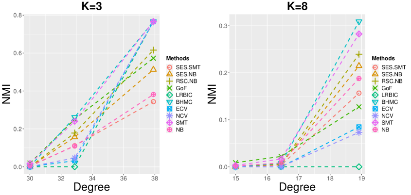
Figure 1: NMI comparison of methods for estimating the number of communities in SBMs at a high out-in ratio. We compiled normalized mutual information across different methods for estimating number of communities in SBMs of network size of $1000$ nodes with the true number of communities $K$ varying over $(3,8)$ while keeping out-in ratio as $0.40$.

Figure 1 suggests that BHMC and SMT are two stand-out methods in the first experiment. For small $K$, we observe that the performance of non-spectral methods are more sensitive to the changes in the degree compared to the non-spectral methods or even hierarchical methods. This is because the spectral methods utilize few eigenvalues to estimate the number of communities, which tend to be more robust with changes in degrees. For large $K$, we see that the performance of non-spectral methods is underwhelming even for higher degrees. This is expected because the non-spectral methods assume the number of communities to be fixed. Figure 1 also suggests that the hierarchical methods have somewhat middling performance.

For the second experiment, we compared the performance of SMT against BHMC and SES.NB, SES.SMT and RSC.NB. We chose hierarchical methods because they had somewhat better performance than the non-spectral methods for large $K$ and the ability of hierarchical methods to estimate a large number of communities, see Li et al. (2020). Like in the first experiment, we generated adjacency matrices $A$ from SBM using (4). In particular, we simulated multiple networks of size $n=5000$ with the fixed out-in ratio as $1/3$ and $0.4$ while we varied the true number of communities over $(10,20,30,60)$ and the degree over $(50,100,150,200)$. Like in the first experiment for every scenario, we generated $100$ copies of adjacency matrices from the SBM and then compiled the normalized mutual information (NMI) of various methods. As discussed before, we kept the significance level as $0.05$. Table 2 compiles the normalized mutual information (NMI) for all the four methods when the out-in ratio was $1/3$. It is immediate that as the true number of communities increases the performance of every method decreases. However, SMT has comparatively better performance in all scenarios. Table 2 in the Supplement gives a similar comparison of results when the out-in ratio was $0.4$. In this scenario too, SMT has a comparatively better performance than the rest of the methods. The slightly improved performance of SMT over BHMC in Table 2 compared to Figure 1 can be attributed to the improved power of SMT as the network size increases. Specifically, in underfitted models as the network size increases one of the candidate eigenvalues corresponding to the candidate Erdös Rényi blocks becomes large enough under the assumption of balanced block sizes (A.1).

Table 2: NMI comparison of methods for estimating the number of communities in SBMs. We compiled the normalized mutual information for estimating the number of communities in networks of size $5000$ for multiple scenarios with the true number of communities ($K$) varying over $(10,20,30,60)$ and the average degree varying over $(50,100,150,200)$ and the out-in ratio was $1/3$.

True $K$	d	SES.NB	RSC.NB	SMT	BHMC
10	50	0.242	0.641	0.946	0.848
20	50	0.082	0.11	0.316	0.193
30	50	0.006	0.006	0.028	0.007
60	50	0	0	0.004	0
10	100	0.384	0.921	0.996	0.935
20	100	0.169	0.524	0.954	0.440
30	100	0.089	0.145	0.477	0.185
60	100	0	0	0.006	0
10	150	0.472	0.972	0.996	0.940
20	150	0.229	0.791	0.980	0.51
30	150	0.135	0.352	0.922	0.290
60	150	0	0	0.042	0
10	200	0.522	0.984	0.995	0.938
20	200	0.273	0.883	0.979	0.528
30	200	0.169	0.606	0.976	0.343
60	200	0.018	0.024	0.153	0.011

For the third scenario, we generated adjacency matrix $A$ according to the BTSBM model in (3.6). For the third experiment, we compared the extension of SMT to hierarchical networks against competing methods for hierarchical networks. For this experiment, we generated adjacency matrices from BTSBM. In this experiement, we varied the depth of the network over $(2,4,6,8)$ while varying the average degree of the network. Moreover, we fixed hierarchical probabilities $(p_{0},\cdots,p_{d})=(a^{0},\cdots,a^{d})$. As discussed before, we used normalized mutual information (NMI) for comparing the performance of all the methods. Table 3 compiles the performance of our method. It is evident from Table 3 that SES.SMT has sub-par performance for small value of true number of communities $K$, but it catches up as the true number of communities $K$ increases to $256$. This is largely because the performance of other methods tapers off as the true number of communities increases.

Table 3: NMI comparison of methods for estimating the number of communities in BTSBM. We compiled the normalized mutual information for estimating the number of communities in networks of size $6400$ for multiple scenarios with the true number of communities ($K$) varying over $(4,16,64,256)$ and $a$ varying over $(0.2,0.4)$ .

True $K$	a	SES.SMT	SES.NB	RSC.NB
4	0.2	0.5	1.000	1.000
16	0.2	0.750	1	1
64	0.2	0.833	1.00	1.000
256	0.2	0.866	0.866	0.874
4	0.4	0.503	1.000	1.000
16	0.4	0.751	0.999	0.999
64	0.4	0.833	1.00	1.000
256	0.4	0.875	0.875	0.875

5 Real Data Analysis

In this subsection, we perform two types of real data analysis. First, we benchmark the performance of SMT against other competing methods on six benchmark scRNA-seq datasets for which the reference clusters are known. Second, we use SMT and HCD-SMT to estimate the clusters in a sparse scRNA-seq datasets.

5.1 Benchmark Data Analysis

For benchmark analysis, we run our comparison analysis on six scRNA-seq datasets that were considered gold-standard in Kiselev et al. (2017). The six reference datasets can be downloaded from Gene Expression Omnibus (GEO) Edgar et al. (2002) with their ascension given in Table 4. For comparison analysis, we run SMT, SC3 (Kiselev et al., 2017), SIMLR (Wang et al., 2018), and SEURAT (Satija et al., 2015) on the six reference datasets. Before running the comparison analysis, we first run data preprocessing steps on the six reference datasets. Subsequently, we processed the scRNA-seq data in line with the current best practices in the existing literature, see Luecken and Theis (2019), Kiselev et al. (2017). The data preprocessing steps were common for all the four methods. In the data preprocessing step, we discarded genes that have low variability. In particular, we kept genes whose variability is at least greater than the $50^{th}$ quantile. Then, we normalized the remaining single-cell data using the $log_{2}(1+x/10000)$ transformation. Subsequently, we ran the rest of the analyses for SC3, SEURAT, and SIMLR using the default parameter settings. Since the filtered benchmark data was fairly dense, therefore for running SMT we generated an adjacency matrix $A$ using the correlation matrix of transformed single-cell data with the $50^{th}$ quantile as the cut-off for forming an edge.

Table 4: Summary of six reference datasets. The following is the summary level information on six reference datasets along with their GEO ascension numbers and the original papers.

Datasets	Number	Number	Cell Resource	GEO ascension	Reference Paper
	of Cells	of Genes		number
Biase	49	25,737	2-cell and 4-cell	GSE57249	Biase et al. (2014)
			mouse embryos
Yan	124	22,687	Human preimplantation	GSE36552	Yan et al. (2013)
			embryos and
			embryonic stem cells
Goolam	124	41,480	4-cell mouse embryos	E-MTAB-3321	Goolam et al. (2016)
			embryos
Deng	268	22,457	Mammalian cells	GSE47519	Deng et al. (2014)
Pollen	301	23,730	Human cerebral cortex	SRP041736	Pollen et al. (2014)
Kolodziejczyk	704	38,653	Mouse embryonic	E-MTAB-2600	Kolodziejczyk et al. (2016)
			stem cells

Post preprocessing, we run SMT, SC3, SEURAT, and SIMLR on the six reference datasets to get estimated cell cluster labels for all the four methods. For SMT, we chose the significance level $\alpha=0.05$. Using the reference cell cluster labels for the six reference datasets and the estimated cell cluster labels, we compute adjusted rand index (ARI) for all four methods across six reference datasets (see Figure 2). Table 5 gives the estimated cell cluster across the six reference datasets along with the reference number of cell clusters.

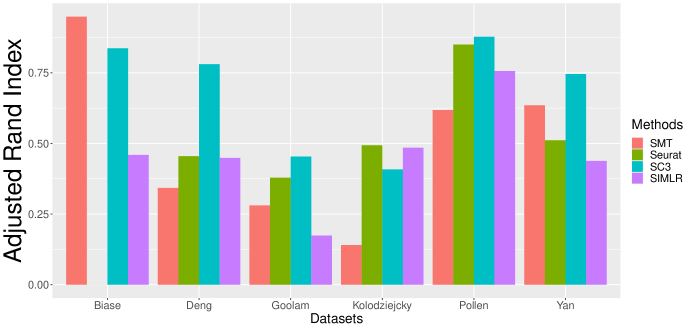
Figure 2: Visual representation of the adjusted rand index computed on reference single-cell datasets. First, we leave out genes whose variability is less than the $50^{th}$ quantile. Second, we normalize the single-cell data by dividing it by $1000$. Third, we transform the single cell data using $log(1+x)$ function. Fourth, we used SMT, Seurat, SC3, and SIMLR to obtain the estimated cell clusters of the six reference datasets, namely: Biase, Deng, Goolam, Kolodziejcky, Pollen, and Yan. Finally, we used original cell clusters (obtained by the respective authors) and the estimated cell clusters to obatin the adjusted rand index for all four methods.

Overall, Figure 2 suggests that SC3 performs well across the six reference datasets, while SMT has middling performance. Table 5 also suggests the same. The performance of SMT is sensitive to SBM assumptions and the choice of $50^{th}$ quantile in forming an edge in adjacency matrices. Selecting the $50^{th}$ quantile is akin to assuming that the network is dense. The rationale for dense network stems from the fact that our pre-processing has selected only the top half of most variable genes and therefore it is safer to assume that filtered scRNA-seq data have less sparsity. However, it is worth noting that increasing the cut-off would increase the sparsity and negatively impact the performance of SMT. Table in the Supplement compares the performance of SMT when the cut-off used is the $95^{th}$ quantile instead of the $50^{th}$ quantile.

Table 5: Comparison table for estimated number of communities for reference single cell datasets.

Datasets	Reference	SMT	SC3	SIMLR
Biase	3	3	3	7
Yan	7	3	6	12
Goolam	5	10	6	19
Deng	10	10	9	16
Pollen	11	11	11	15
Kolodziejcky	3	27	10	6

5.2 Sparse Single-cell Data Analysis

For the rest of the data analysis, we use scRNA-seq data generated from the retina cells of two healthy adult donors. The scRNA-seq data was generated from the retina cells of two healthy adult donors using the 10X Genomics Chromium^TM system. Detailed preprocessing and donor characteristics of our scRNA-seq data can be found in Lyu (2019) (see Supplementary Note 1). In total, 33694 genes were sequenced over 92385 cells. The sequencing data were initially analyzed with R package Seurat (Satija et al. (2015)) and every cell was identified as a particular cell type. Table 3 in the supplementary material gives the relative size of these cell types.

For sparse single-cell data analysis, we consider two types of data analysis: i) Composite data analysis, ii) Subgroup analysis of bipolar cells. In composite data analysis, we combine different single cells with classification known from Seurat and then we use SMT to retrieve the estimated number of cell clusters. The composite analysis aimed to see if we can recover the true number of cell clusters when the number of true cell clusters was well-known in advance. In the subgroup analysis, we use the hierarchical version of SMT (SES.SMT) for the clustering of bipolar cells. The rationale for clustering bipolar cells using SES.SMT is that the bipolar cells have multiple subgroups with the possibility of having a hierarchical structure.

For composite data analysis, we analyzed subsets of Ganglion, Endothelium, Cone, Bipolar, Horizontal, and Rod cell types. The composite network was obtained by combining equal samples of size $500$ from each of the above cell types. For the above network, we used correlations between cells to compute similarity between cells. Subsequently, we used the correlation matrix with $95^{th}$ quantile (of entries of the correlation matrix) as the cutoff to generate an adjacency matrix. Subsequently, we used SMT to estimate the number of communities. The rationale for running SMT was the composite data was artifically constructed as composition of six different cell types. SMT and BHMC estimated the number of communities as six whereas LRBIC, ECV, NCV estimated the number of communities as $25$, $29$, and $29$ respectively. It is evident that both SMT and BHMC recovered the true number of cell clusters in the composite network. Figure 3 gives the t-SNE plot for the estimated composite network.

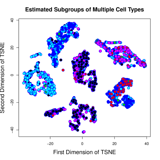
Figure 3: Visual representation of the estimated clusters of the composite scRNA-seq data of human retina cells in the t-SNE plot. The composite scRNA-seq data was obtained from the scRNA-seq data of human retina cells by selecting Seurat classified cell types namely: Ganglion, Endothelium, Cone, Bipolar, Horizontal, and Rod cells in an equal manner of roughly $500$ cells per cell type. The composite network data was generated by assigning the edge between a pair of cells whenever the correlation between the two cells was greater than the $(1-\rho_{n})^{th}$ quantile of the elements of the sample correlation matrix, where $\rho_{n}=0.05$. Subsequently, using SMT, we obtained the estimate of the number of communities in the composite network data as six. Also, we used the sample correlation matrix to generate the t-SNE plot. The estimated clusters are shown using different colors in the t-SNE plot.

Our scRNA-seq data of bipolar cells was given in a matrix form with genes denoting the rows and cells denoting the columns. In total, we had $33,694$ genes and $30,125$ cells. Subsequently, we processed the scRNA-seq data in line with the current best practices in the existing literature, see Luecken and Theis (2019), Kiselev et al. (2017). In particular, we filtered out genes whose variability was less than the $50^{th}$ quantile. And we filtered out cells whose total cell counts (across all genes) were less than $500$ and greater than $2500$. Subsequently, we normalized the data using $log_{2}(1+x/10000)$. Then, we computed the correlation matrix between the cells. Using the correlation matrix and the $95^{th}$ quantile of entries of the sample correlation matrix as the cutoff to generate the adjacency matrix. We used the cut-off $95^{th}$ quantile of the entries of the sample correlation matrix to keep the sparsity in the range of theoretical value of the sparsity parameter for which SMT holds. Then, we used the hiearchical version of SMT (i.e., SES.SMT) to estimate the number of communities. The rationale for selecting SES.SMT was that the bipolar cell types are believed have to number of subgroups with possiblly hiearchical structure. Figure 4 plots the estimated subgroups of single cells along the two dimensions of t-SNE. The estimated subgroups in the figure appear as clustered with a hierarchy. The comparison of highly expressed genes of the subgroups of bipolar cells of a healthy patient against the highly expressed genes of the subgroups of bipolar cells of a diseased patient can potentially help uncover driver genes (Myers et al., 2015).

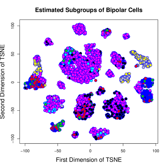
Figure 4: Visual representation of estimated subgroups of bipolar cell types of human retina single-cells in the t-SNE plot. The bipolar single cells from the original scRNA-seq of retina cells were selected using the Seurat classified cell types. The bipolar cells were then filtered and normalized using the general data manipulating strategies for scRNA-seq datasets. Subsequently, we computed the sample correlation matrix and the network data was generated by assigning an undirected edge between a pair of cells when the correlation between the two cells was greater than the $95^{th}$ quantile of the entries of the sample correlation matrix. Then, we used the hierarchical extension of SMT (i.e., SES.SMT) to estimate the number of communities. The estimated subgroups are denoted by different colors in the t-SNE plot.

6 Discussion

In summary, SMT is useful for estimating the number of communities in sparse and large SBMs. Moreover, SMT can be adapted as a stopping rule for BTSBMs. The main advantage of SMT over other competing approaches is it has broad theoretical guarantees for sparse SBMs while allowing the number of communities to increase with the network size. This has wider implications for application areas such as clustering of large scRNA-seq datasets where assuming a fixed number of communities could be limiting. Moreover, SMT can estimate the number of communities increasing at the order of $O(n^{1/4})$, which is much higher than the $O(n^{1/6})$ that the GoF method of Lei (2016) can estimate.

A drawback of SMT is that it does not automatically extend to the DCSBMs. The main argument behind this assertion is that SMT uses the fact that all but the top eigenvalues of appropriately scaled adjacency matrices under the null converges to the semi-circular distribution which is not necessarily true for the corresponding scaled adjacency matrices for the blocks/communities of DCSBMs. There is a possibility to have a SMT-like procedure for estimating the number of blocks in DCSBMs provided that we could characterize non-homogenous Erdös Rényi block in terms of its spectral properties.

Supplementary Materials The Supplement includes proofs and additional information related to real datasets used for the analysis.

References

- Airoldi et al. (2008) Airoldi, E. M., D. M. Blei, S. E. Fienberg, and E. P. Xing (2008). Mixed membership stochastic blockmodels. Journal of Machine Learning Research 9, 1981–2004.
- Amini et al. (2013) Amini, A. A., A. Chen, P. J. Bickel, and E. Levina (2013). Pseudo-likelihood methods for community detection in large sparse networks. Annals of Statistics 41(4).
- Amini and Levina (2018) Amini, A. A. and E. Levina (2018). On semidefinite relaxations for the block model. Annals of Statistics 46(1), 149–179.
- Balakrishnan et al. (2011) Balakrishnan, S., M. Xu, A. Krishnamurthy, and A. Singh (2011). Noise thresholds for spectral clustering. Advances in Neural Information Processing Systems, 954–962.
- Biase et al. (2014) Biase, F. H., X. Cao, and S. Zhong (2014). Cell fate inclination within 2-cell and 4-cell mouse embryos revealed by single-cell rna sequencing. Genome Res. 24, 1787–1796.
- Bickel and Chen (2009) Bickel, P. J. and A. Chen (2009). A nonparametric view of network models and newman-girvan and other modularities. Proceedings of the National Academy of Sciences of the United States of America 106(50), 21068–21073.
- Blondel et al. (2008) Blondel, V. D., J.-L. Guillaume, R. Lambiotte, and E. Lefebvre (2008). Fast unfolding of communities in large networks. Journal of Statistical Mechanics Theory and Experiment.
- Chaudhuri et al. (2012) Chaudhuri, K., F. Chung, and A. Tsiatas (2012). Spectral clustering of graphs with general degrees in the extended partition model. JMLR : Workshop and Conference Proceedings vol, 35.1–35.23.
- Chen and Lei (2018) Chen, K. and J. Lei (2018). Network cross-validation for determining the number of communities in network data. Journal of the American Statistical Association 113(521).
- Choi et al. (2012) Choi, D. S., P. J. Wolfe, and E. M. Airoldi (2012). Stochastic blockmodels with a growing number of classes. Biometrika 99(2), 273–284.
- Clauset et al. (2008) Clauset, A., C. Moore, and M. E. J. Newman (2008). Hierarchical structure and the prediction of missing links in networks. Nature 453, 98–101.
- Deng et al. (2014) Deng, Q., D. Ramsköld, B. Reinius, and R. Sandberg (2014). Single-cell rna-seq reveals dynamic, random monoallelic gene expression in mammalian cells. Science 343, 193–196.
- Ding et al. (2016) Ding, Z., X. Zhang, and B. Luo (2016). Overlapping community detection based on network decomposition. Scientific Reports 6(24115).
- Eberwine et al. (2014) Eberwine, J., S. Jai-Yoon, T. Bartfai, and J. Kim (2014). The promise of single cell sequencing. Nature Methods 11(1), 25–27.
- Edgar et al. (2002) Edgar, R., M. Domrachev, and L. A.E. (2002). Gene expression omnibus: Ncbi gene expression and hybridization array data repository. Nucleic Acids Res. 30(1), 207–210.
- Gao et al. (2017) Gao, C., Z. Ma, A. Y. Zhang, and H. H. Zhou (2017). Achieving optimal misclassification proportion in stochastic block models. The Journal of Machine Learning Research 18(1), 1980–2024.
- Goolam et al. (2016) Goolam, M., A. Scialdone, S. J. L. Graham, I. C. MacAulay, and A. Jedrusik (2016). Heterogeneity in oct4 and sox2 targets biases cell fate in 4-cell mouse embryos. Cell 165, 61–74.
- Holland et al. (1983) Holland, P. W., K. B. Laskey, and S. Leinhardt (1983). Stochastic block models: First steps. Social Networks 5, 109–137.
- Hou et al. (2020) Hou, W., Z. Ji, H. Ji, and S. Hicks (2020). A systematic evaluation of single-cell rna-sequencing imputation methods. Genome Biology 21(218).
- Joseph and Yu (2016) Joseph, A. and B. Yu (2016). Impact of regularization on spectral clustering. Annals of Statistics 44(4), 1765–1791.
- Karrer and Newman (2011) Karrer, B. and E. J. Newman (2011). Stochastic blockmodels and community structure in networks. Physics Review E 83(1).
- Kiselev et al. (2019) Kiselev, V. Y., T. S. Andrews, and M. Hemberg (2019). Chalenges in unsupervised clustering of single-cell rna-seq data. Nature Reviews Genetics 20, 273–282.
- Kiselev et al. (2017) Kiselev, V. Y., K. Kirschner, M. T. Schaub, T. Andrews, A. Yiu, T. Chandra, K. N. Natarajan, W. Reik, M. Barahona, A. R. Green, and M. Hemberg (2017). Sc3: consensus clustering of single-cell rna-seq data. Nature Methods 14, 483–486.
- Kiselev et al. (2017) Kiselev, V. Y., K. Kristina, M. T. Schaub, and T. e. a. Andrews (2017). Sc3- consensus clustering of single-cell rna-seq data. Nature Methods 14(5), 483–486.
- Kolodziejczyk et al. (2016) Kolodziejczyk, A. A., J. K. Kim, J. C. H. Tsang, T. Ilicic, and J. Henriksson (2016). Single cell rna-sequencing of pluripotent states unlocks modular transcriptional variation. Cell Stem Cell 17, 471–485.
- Lancichinetti and Fortunato (2009) Lancichinetti, A. and S. Fortunato (2009). Community detection algorithms : A comparative analysis.
- Lee and Levina (2015) Lee, C. M. and E. Levina (2015). Estimating the true number of communities in networks by spectral methods. arXiv, https://arxiv.org/pdf/1507.00827.pdf.
- Lee and Schnelli (2018) Lee, J. O. and K. Schnelli (2018). Local law and tracy-widom limit for sparse random matrices. Probability Theory and Related Fields 171, 543–616.
- Lei (2016) Lei, J. (2016). A goodness-of-fit test for stochastic block models. The Annals of Statistics 44(1), 401–424.
- Lei and Rinaldo (2015) Lei, J. and A. Rinaldo (2015). Consistency of spectral clustering in sparse stochastic block models. Annals of Statistics 43(1), 215–237.
- (31) Lei, J. and L. Zhu. A generic sample splitting approach for refined community recovery in stochastic block models. Preprint. Available at arXiv:1411.1469.
- Li et al. (2020) Li, T., L. Lei, S. Bhattacharya, K. V. d. Berge, P. Sarkar, P. J. Bickel, and E. Levina (2020). Hierarchical community detection by recursive partitioning. Journal of the American Statistical Association.
- Li et al. (2016) Li, T., E. Levina, and J. Zhu (2016). Network cross-validation by edge sampling. arXiv preprint arXiv:1612.04717.
- Luecken and Theis (2019) Luecken, M. D. and F. J. Theis (2019). Molecular Systems Biology 15(6).
- Lyu (2019) Lyu, Y. e. a. (2019). https://www.biorxiv.org/content/10.1101/768143v1.full;bioarXiv.
- Ma et al. (2019) Ma, S., L. Su, and Y. Zhang (2019). Determining the number of communities in degree-corrected stochastic block models. arXiv:https://arxiv.org/pdf/1809.01028.pdf.
- Myers et al. (2015) Myers, J., A. von Lersner, C. Robbins, and Q.-X. Sang (2015). Differentially expressed genes and signature pathways of human prostate cancer. PLoS One, 10:e0145322.
- Newman and Girvan (2004) Newman, M. E. J. and M. Girvan (2004). Finding and evaluating community structures in networks. Physical Review E 69, 026113.
- Peel and Clauset (2015) Peel, L. and A. Clauset (2015). Detecting change points in the large-scale structure of evolving networks. AAAI, 2914–2920.
- Pollen et al. (2014) Pollen, A. A., T. J. Nowaowski, J. Shuga, X. Wang, and A. A. Leyrat (2014). Low-coverage single-cell mrna sequencing reveals cellular heterogeneity and activating signalling pathways in developing cerebral cortex. Nat Biotechnology 32, 1053–1058.
- Qin and Rohe (2013) Qin, T. and K. Rohe (2013). Regularized spectral clustering under the degree-corrected stochastic blockmodel. NIPS.
- Rohe et al. (2011) Rohe, K., S. Chatterjee, and B. Yu (2011). Spectral clustering and the high-dimensional stochastic blockmodel. The Annals of Statistics 39(4), 1878–1915.
- Satija et al. (2015) Satija, R., J. A. Farrell, D. Gennert, A. F. Schier, and A. Regev (2015). Spatial reconstruction of single-cell gene expression data. Nature Biotechnology 33(5), 495–502.
- Svensson et al. (2020) Svensson, V., E. d. V. Beltrame, and L. Pachter (2020). A curated database reveals trends in single-cell transcriptomics. Database https://doi.org/10.1093/database/baaa073.
- Wang et al. (2018) Wang, B., D. Ramazzotti, L. D. Sano, J. Zhu, E. Pierson, and S. Batzoglou (2018). Simlr: A tool for large-scale genomic analyses by multi-kernel learning. Proteomics 10.1002/pmic.201700232 18(2).
- Wang and Bickel (2017) Wang, R. Y. X. and P. J. Bickel (2017). Likelihood-based model selection for stochastic block models. The Annals of Statistics 45(2), 500–528.
- Yan et al. (2013) Yan, L., M. Yang, H. Guo, L. Yang, and J. Wu (2013). Single-cell rna-seq profiling of human preimplantation embryos and embryonic stem cells. Nat Struct Mol Biol 20, 1131–1139.
- Zhao (2017) Zhao, Y. (2017). A survey on theoretical advances of community detection in networks. WIREs Comput Stat 9, c1403.
- Zhao et al. (2012) Zhao, Y., E. Levina, and J. Zhu (2012). Consistency of community detection in networks under degree-corrected stochastic block models. The Annals of Statistics 40(4), 2266–2292.