Nonabelian lattice theories: Consistent measures and strata

Abstract

The role of consistent measures in the rigorous construction of nonabelian lattice theories is analized. General conditions that measures must fulfill to insure consistency, positivity and a mass gap are obtained. The impact of nongeneric strata on the nature of the Hamiltonian lattice potential is also discussed.

1 Introduction

There are two ways to look at lattice theories. In one of them, to characterize a theory in the continuum one starts from a discretized spacetime, with a finite lattice of points and then, by successively decreasing the lattice spacing $a$ and increasing the total volume $V$ of the lattice, one approaches the continuum theory. At each step, taking an Euclidean point of view, the discrete approximation of theory rests defined by the choice of a measure. There is no need for these intermediate measures to have a well defined physical meaning. All that is required is that in the limit $a\rightarrow 0$ and $V\rightarrow\infty$ one obtains the desired continuum measure. Of course, because in the limit one is dealing with the delicate problem of measures in infinite dimensional spacetimes, the choice of the intermediate finite dimensional measures turns out to be important to insure the existence of the limit measure. However this is only a requirement of mathematical convenience.

An alternative way to look at lattice theories is to consider the lattice as an observational scaffold of some unknown theory which may or may not be defined in the continuum, either because it possesses some intrinsic validity cutoff or even because the spacetime manifold changes its nature at small distances [1] [2] [3]. In this latter case the definition of the lattice and its associate measure is much less arbitrary, because at each step one requires an exact description of the theory at the length scale of the lattice.

In both instances, whether as a device to approach the continuum limit or a scaffold to define the theory at all length scales, the mathematical notion of consistent measure (to be defined in the next subsection) is the appropriate tool. In the first case because it insures the existence of a limit measure and in the second because it insures probabilistic consistency in the description of the physical system at all length scales.

Another important point in the formulation of nonabelian gauge theories is the fact that in these theories the configuration space as well as the phase space are not manifolds but orbifolds with singular points corresponding to states of higher symmetry [4] [5]. Therefore the characterization of their strata is important in particular because they might correspond to a multiplicity of condensate backgrounds or potential minima. A multiplicity of backgrounds might lead to a multiplicity of solutions in the (Schwinger-Dyson) gap equation for fermion mass generation [6] [7]. The nature of the gauge strata in the nonabelian lattice theories will be analyzed. Because quantum wave functions naturally explore different strata, the impact of nongeneric strata on the backgrounds spectrum is related to the nature of the lattice potential associated to the measure.

1.1 Projective limits and consistent measures as tools to approach the continuum or to describe physical systems at all scales

The definition of consistent measures on a sequence of spaces (lattices in this case) requires that the sequence be defined in an appropriate way. This leads to the notion of:

Projective limit

Let $(I,\preceq)$ be a directed set and $\left\{X_{i};i\in I\right\}$ a family of topological separable spaces indexed by $I$. For every pair $i,j\in I$ with $i\preceq j$ there is a continuous map $\pi_{ij}:X_{j}\rightarrow X_{i}$ such that

$$\pi_{ij}\circ\pi_{jk}=\pi_{ik}\hskip 28.45274pt\text{for\hskip 28.45274pt}i\preceq j\preceq k$$ (1)

This is called a projective family of spaces.

The projective limit of the family is the subset $X$ of elements of the Cartesian product $\Pi_{i\in I}X_{i}$ such that its elements $x=\left(x_{i}\right)$ satisfy

$$x_{i}=\pi_{ij}x_{j}\hskip 28.45274pt\text{for\hskip 28.45274pt}i\preceq j$$ (2)

Furthermore there are mappings $\pi_{i}:X\rightarrow X_{i}$ such that

$$\pi_{i}=\pi_{ij}\circ\pi_{j}\hskip 28.45274pt\text{for\hskip 28.45274pt}i\preceq j$$ (3)

The projective limit $X$ is denoted

$$X=\underleftarrow{\lim}X_{i}$$ (4)

Consistent measures

Of special interest is the case where each space $X_{i}$ is equipped with a probability measure $\mu_{i}$. The family of measures $\left\{\mu_{i}\right\}$ is called a consistent family if for every measurable set $A$ in $X_{i}$

$$\mu_{i}\left(A\right)=\mu_{j}\left(\pi_{ij}^{-1}\left(A\right)\right)\hskip 28.45274pt\text{for\hskip 28.45274pt}i\preceq j$$ (5)

The measure on the projective limit

The next question is to know when, given a consistent family of measures, there is also a measure $\mu$ on the projective limit $X$. The most general requirement is probably the following [8] [9]:

For every $\varepsilon>0$ there is a compact subset $K\subset X$ such that

$$\mu_{i}\left(X_{i}\setminus\pi_{i}\left(K\right)\right)\leq\varepsilon\hskip 28.45274pt\text{for every }i\in I$$ (6)

and $\mu$ is denoted

$$\mu=\underleftarrow{\lim}\mu_{i}$$ (7)

The existence of an infinite-dimensional measure as a limit of consistent finite-dimensional measures is a powerful concept in the sense that the limit measure might even be of different nature from the finite-dimensional ones, for example not being absolutely continuous in relation to the reference measure of the finite-dimensional ones.

A classical illustration of these concepts is Kolmogorov’s construction of a stochastic process $\left\{X_{t}:t\in\mathbb{R}^{+}\right\}$ from its finite-dimensional distributions [10]:

Here $I=\mathbb{R}^{+}$, the $X_{i}$ spaces are discrete subsets $\left\{t_{1},t_{2},\cdots,t_{n}\right\}$ of $\mathbb{R}^{+}$ ordered by inclusion with measures $\mu_{t_{1},t_{2},\cdots,t_{n}}$ being the finite-dimensional probability distributions. The mappings $\pi_{ij}$ are simply the coordinate projections from the sets $\left\{t_{1},t_{2},\cdots,t_{n}\right\}$ to its subsets. One important point to notice in this construction is that the projective limit (a subset of the Cartesian product) is not simply the continuum limit of the stochastic process, instead it also contains, in a consistent manner, the description of the process at all levels of observation.

In this paper this framework will be applied to the description of physical systems extended in space-time, that is fields. Therefore it is natural to consider the directed set to be a space-time lattice that, by subdivision of its length elements, is successively refined and ordered by inclusion. Notice that there is no need to identify the lattice with the physical system, the lattice might simply be a observational scaffold of the physical system at successively smaller scales. There is also no need to assume that the physical systems are defined up to arbitrarily smaller scales. The directed set $I$ may very well stop at some nonzero scale. The definition of the sequence of spaces and their mappings is not particularly difficult. The important point is of course to find the consistent measures relevant to each physical system.

1.2 Heat kernels

Heat kernels are wonderful mathematical objects and, as has been pointed out before [11] [12], appear in all manner of places and disguises. But where does the wonderfulness of heat kernels come from?

Given the operator $-O_{x}+\frac{\partial}{\partial t}$ where the operator $O$ is an elliptic operator, in particular a Laplacian in $\mathbb{R}^{n}$, on a manifold or on a group manifold, the heat kernel is the solution of the equation

$$\left(-O_{x}+\frac{\partial}{\partial t}\right)K_{t}\left(x,y\right)=0$$ (8)

What makes the heat kernel a powerful gadget is the convolution approximating property

$$\lim_{n\rightarrow\infty}K_{\frac{1}{n}}\ast f=f$$ (9)

$f$ being a continuous and bounded function, as well as its representation as a theta series

$$K\left(t,x,y\right)=\sum_{k}\phi_{k}\left(x\right)\phi_{k}\left(y\right)e^{-\lambda_{k}t}$$ (10)

for a manifold, with the $\phi_{k}^{\prime}s$ being a complete orthonormal set of eigenvectors of the Laplacian and $\left\{\lambda_{k}\right\}$ the set of their eigenvalues or a similar expression for a group manifold with $x$ and $y$ group elements and the $\phi_{k}^{\prime}s$ representation characters. Another important property, which naturally follows from the evolution equation (8) is the convolution semigroup property

$$K_{t_{1}}\ast K_{t_{2}}=K_{t_{1}+t_{2}}$$ (11)

This property turns out to be of critical importance for the construction of consistent measures. Notice also that a large family of convolution semigroups of the heat kernel type do exist not only associated to Laplacians but also to other more general Lévy kernels [13].

1.3 A projective lattice family for spacetime fields

In $n$-dimensional spacetime consider a set $\left(\mathcal{L},\preceq\right)$ of successively finer hypercubic lattices ordered by inclusion. Starting from some initial hypercubic lattice $L_{0}$ with lattice spacing $a_{0}$, the successive elements $L_{i}\in\mathcal{L}$ in this ordered set are obtained both by regular subdivision of already existent plaquettes as well as by the addition of new square or rectangular plaquettes. For the purpose of definition of the mappings $\pi_{ij}:L_{j}\rightarrow L_{i}$ with $i\preceq j$ the elementary sets are the plaquettes, the plaquettes in $L_{j}$ being mapped on the corresponding plaquettes on $L_{i}$ or on the empty set when they are new plaquettes which do not correspond to a subdivision of the plaquettes in $L_{i}$. (this is analogous to the coordinate projections in the Kolmogorov construction). The property $\pi_{ij}\circ\pi_{jk}=\pi_{ik}$ for $i\preceq j\preceq k$ being verified, a projective family of lattices is obtained, with projective limit defined as the subset $L$ of elements of the Cartesian product $\Pi_{i\in I}L_{i}$ such that its elements $L=\left(L_{i}\right)$ satisfy

$$L_{i}=\pi_{ij}L_{j}\hskip 28.45274pt\text{for\hskip 28.45274pt}i\preceq j$$ (12)

It should be pointed out that the family of lattices may either be infinite if the lattice spacing $a_{n}\rightarrow 0$ and (or) the total volume $V\rightarrow\infty$ or finite for finite volume and finite cutoff $a_{c}$.

1.4 Strata [14], [15], [16]

Let $G$ be a compact Lie group acting on a manifold $\mathcal{M}$. The action of $G$ on $\mathcal{M}$ leads to a stratification of $\mathcal{M}$ corresponding to the classes of equivalent orbits $\left\{g\mathcal{M};g\in G\right\}$. Let $S_{x}$ denote the isotropy (or stabilizer) group of $x\in\mathcal{M}$

$$S_{x}=\left\{\gamma\in G:\gamma x=x\right\}$$ (13)

The stratum $\Sigma\left(x\right)$ of $x$ is the set of points having isotropy groups $G-$conjugated to that of $x$

$$\Sigma\left(x\right)=\left\{y\in\mathcal{M}:\exists\gamma\in G:S_{y}=\gamma S_{x}\gamma^{-1}\right\}$$ (14)

If $G$ is a symmetry group for a physical system with states in $\mathcal{M}$, the configuration space of the system is the quotient space $\mathcal{M}/G$ and a stratum is the set of points in $\mathcal{M}/G$ that corresponds to orbits with conjugated isotropy groups. The map that, to each orbit, assigns the conjugacy class of its isotropy group is called the type. The set of strata carries a partial ordering of types, $\Sigma_{x}\subseteq\Sigma_{x^{\prime}}$ if there are representatives $S_{x}$ and $S_{x^{\prime}}$ of the isotropy groups such that $S_{x}\supseteq S_{x^{\prime}}$. The maximal element in the ordering of types is the class of the center $Z(G)$ of $G$ and the minimal one is the class of $G$ itself.

In gauge theories, one deals with the strata of the connections, the strata being in one-to-one correspondence with the Howe subgroups of $G$, that is, the subgroups that are centralizers of some subset in $G$. Given an holonomy group $H_{\tau}$ associated to a connection $A$ of type $\tau$, the stratum of $A$ is classified by the conjugacy class of the isotropy group $S_{\tau}$, that is, the centralizer of $H_{\tau}$,

$$S_{\tau}=Z\left(H_{\tau}\right)$$ (15)

an important role being also played by the centralizer of the centralizer

$$H_{\tau}^{\prime}=Z\left(Z\left(H_{\tau}\right)\right)$$ (16)

that contains $H_{\tau}$ itself. If $H_{\tau}^{\prime}$ is a proper subgroup of $G$, the connection $A$ reduces locally to the subbundle $P_{\tau}=\left(\mathcal{M},H_{\tau}^{\prime}\right)$.  Whether or not all the strata types exist for the action of $G$ on $\mathcal{M}$ depends on the structure of $\mathcal{M}$ itself. Global reduction depends on the topology of $\mathcal{M}$, but it is always possible if $P=\left(\mathcal{M},G\right)$ is a trivial bundle. $H_{\tau}^{\prime}$ is the structure group of the maximal subbundle associated to type $\tau$. Therefore the types of strata are also in correspondence with types of reductions of the connections to subbundles. If $S_{\tau}$ is the center of $G$ the connection is called irreducible, all others are called reducible. The stratum of the irreducible connections is called the generic stratum. It is open and dense.

1.5 Summary of results

In Refs.[17] and [18], by using measures that satisfy a semigroup law, it was possible to check the consistency of the measures at the one-plaquette level. Here the construction is extended for plaquettes sharing common edges, which by induction implies the possibility to construct pure gauge consistent measures in finite or infinite lattices. This is the done in Section 2. The positivity of the transfer matrix and the existence of a mass gap is also established. Then Section 3 explores the construction of consistent measures when there are also fermion matter fields in the lattice. Consistency of a particular measure is checked, here however only at the one-plaquette level. Finally in Section 4 one discusses the role of non-generic strata in lattice theories.

2 Nonabelian pure gauge lattice theory: A review and some developments

Here I will draw and extend the results already obtained in Refs. [17] and [18] concerning the construction of a consistent measure, with also some new results concerning the positivity of the measures as well as an alternative discussion of the mass gap.

2.1 Consistent interacting measures

A state of the nonabelian theory corresponds to the assignment of an element $g$ of a nonabelian group $G$ to each edge of the lattice. As a reference measure, the Haar measure of the group $G$ is also associated to each edge. The set of independent Haar measures in the edges clearly establish a consistent family of measures in the lattice and therefore there also exists a reference Haar measure in the projective limit. In addition the theory is invariant under a direct product group

$$\mathcal{G}=\underset{vertices}{\Pi}G_{i}$$ (17)

that is, an independent copy of $G$ at each vertex which acts on the $ij$ edge group variable $g$ as

$$g\rightarrow g_{i}gg_{j}^{-1}$$ (18)

The next step is to find nontrivial measures, that is measures that couple the group elements in different edges, but that satisfy the consistency requirement along the projective lattice family. In particular one looks for densities that multiply the reference Haar measure. In [17] and [18] this was achieved by considering the construction of the projective family in such a way that at each step only one plaquette is subdivided, together with the adding of new plaquettes. However the procedure is much more general, with the same consistency condition being obtained for the measure densities. If the subdivided plaquettes have no edge in common the proof of the condition for consistency of the measure applies without any modification. The other possibility is when the plaquettes that are subdivided have a common edge. Here I will show that the measure consistency condition is unaltered. This is done by explicit calculation. Consider the two subdivided plaquettes in Fig.1

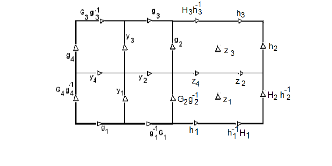
Figure 1: Subdivision of two contiguous plaquettes

The measure density associated to the plaquettes is a central function of the product of the group elements around the plaquettes and denote by $p\left(G_{1}G_{2}G_{3}^{-1}G_{4}^{-1}\right)$ and $p\left(H_{1}H_{2}H_{3}^{-1}G_{2}^{-1}\right)$ the densities associated to the large plaquettes and by $p^{\prime}$ the corresponding densities of the small plaquettes. Furthermore assume that the densities, in addition to being central functions, satisfy the following semigroup properties

$$\int p^{\prime}\left(G_{i}X\right)p^{\prime}\left(X^{-1}G_{j}\right)d\mu_{H}\left(X\right) = p^{\prime\prime}\left(G_{i}G_{j}\right)$$

$$\int p^{\prime\prime}\left(G_{i}X\right)p^{\prime\prime}\left(X^{-1}G_{j}\right)d\mu_{H}\left(X\right) = p\left(G_{i}G_{j}\right)$$ (19)

Then

$$\int p^{\prime}\left(g_{1}y_{1}y_{4}^{-1}g_{4}G_{4}^{-1}\right)p^{\prime}\left(g_{1}^{-1}G_{1}G_{2}g_{2}^{-1}y_{2}^{-1}y_{1}^{-1}\right)p^{\prime}\left(y_{4}y_{3}g_{3}G_{3}^{-1}g_{4}^{-1}\right)p^{\prime}\left(y_{2}g_{2}g_{3}^{-1}y_{3}^{-1}\right)$$ (20)

$$\times p^{\prime}\left(h_{1}z_{1}z_{4}^{-1}g_{2}G_{2}^{-1}\right)p^{\prime}\left(h_{1}^{-1}H_{1}H_{2}h_{2}^{-1}z_{2}^{-1}z_{1}^{-1}\right)p^{\prime}\left(z_{4}z_{3}h_{3}H_{3}^{-1}g_{2}^{-1}\right)p^{\prime}\left(z_{2}h_{2}h_{3}^{-1}z_{3}^{-1}\right)$$

$$\times\prod_{i=1,\cdots,4}d\mu_{H}\left(g_{i}\right)d\mu_{H}\left(y_{i}\right)d\mu_{H}\left(z_{i}\right)d\mu_{H}\left(G_{i}\right)\prod_{j=1,\cdots,3}d\mu_{H}\left(h_{j}\right)d\mu_{H}\left(H_{j}\right)$$

$$= \int p^{\prime}\left(X_{1}X_{4}^{-1}G_{4}^{-1}\right)p^{\prime}\left(X_{1}^{-1}G_{1}G_{2}X_{2}\right)p^{\prime}\left(X_{3}G_{3}^{-1}X_{4}\right)p^{\prime}\left(X_{2}^{-1}X_{3}^{-1}\right)$$

$$\times p^{\prime}\left(Y_{1}Y_{4}^{-1}G_{2}^{-1}\right)p^{\prime}\left(H_{1}H_{2}Y_{2}Y_{1}^{-1}\right)p^{\prime}\left(Y_{3}H_{3}^{-1}Y_{4}\right)p^{\prime}\left(Y_{2}^{-1}Y_{3}^{-1}\right)$$

$$\times\prod_{i=1,\cdots,4}d\mu_{H}\left(X_{i}\right)d\mu_{H}\left(Y_{i}\right)d\mu_{H}\left(G_{i}\right)\prod_{j=1,\cdots,3}d\mu_{H}\left(H_{j}\right)$$

$$= \int p^{\prime\prime}\left(X_{4}^{-1}G_{4}^{-1}G_{1}G_{2}X_{2}\right)p^{\prime\prime}\left(X_{2}^{-1}G_{3}^{-1}X_{4}\right)p^{\prime\prime}\left(H_{1}H_{2}Y_{2}Y_{4}^{-1}G_{2}^{-1}\right)p^{\prime\prime}\left(Y_{2}^{-1}H_{3}^{-1}Y_{4}\right)$$

$$\times d\mu_{H}\left(X_{1}\right)d\mu_{H}\left(X_{2}\right)d\mu_{H}\left(X_{4}\right)d\mu_{H}\left(Y_{2}\right)d\mu_{H}\left(Y_{4}\right)\prod_{i=1,\cdots,4}d\mu_{H}\left(G_{i}\right)\prod_{j=1,\cdots,3}d\mu_{H}\left(H_{j}\right)$$

$$= \int p\left(G_{3}^{-1}G_{4}^{-1}G_{1}G_{2}\right)p\left(H_{3}^{-1}G_{2}^{-1}H_{1}H_{2}\right)\prod_{i=1,\cdots,4}d\mu_{H}\left(G_{i}\right)\prod_{j=1,\cdots,3}d\mu_{H}\left(H_{j}\right)$$

The first step uses centrality, invariance of the Haar measure and the change of variables

$$X_{1} = g_{1}y_{1};X_{2}=g_{2}^{-1}y_{2}^{-1};X_{3}=y_{3}g_{3};X_{4}=g_{4}^{-1}y_{4}$$

$$Y_{1} = h_{1}z_{1};Y_{2}=h_{2}^{-1}z_{2}^{-1};Y_{3}=z_{3}h_{3};Y_{4}=g_{2}^{-1}z_{4}$$ (21)

and the second and the third the semigroup properties (19). This an explicit check of the consistency condition (5).

A quite similar construction holds if the new plaquette that is subdivided shares other edges with other already subdivided plaquettes. By induction, with the reasoning here and in Ref.[17] it is established that:

Proposition 1

Let $\mathcal{L}$ be a (finite or infinite)projective lattice family of compact nonabelian gauge theory with the product Haar measure as reference measure. Then a sufficient condition for the existence of a consistent measure in $\mathcal{L}$ is that the (plaquette) densities be central functions satisfying the semigroup conditions (19).

Notice that in (19) the equality sign might be simply replaced by ”proportional to”, with the scaling factor being absorbed by the measure normalization.

The choice of the semigroup defines the particular physical theory that is implemented (or observed) in the lattice. In [17] and [18] it has been checked that the heat kernel associated to the group $G$ , having the semigroup properties (11) it also approximates at small lattice spacing the formal measure associated to the Yang-Mills Lagrangian. It might therefore be used as a rigorous definition of this as yet undefined theory. In this case then, the measure density associated to each plaquette is the heat kernel $K\left(U_{\square},\beta\right)$.

From the consistency condition one sees that as the plaquettes are subdivided along the consistent family of lattices, one should replace the $\beta$ parameter in the heat kernel associated to each particular plaquette in the following way:

$$\beta \rightarrow \beta^{\prime}=\frac{\beta}{4}\hskip 28.45274pt\text{for subdivision of one }a-\text{plaquette into }4\text{ }a/2-\text{plaquettes}$$

$$\beta \rightarrow \beta^{\prime\prime}=\frac{\beta}{2}\hskip 28.45274pt\text{for subdivision of one }a-\text{plaquette into }2\text{ rectangular plaquettes}$$

Hence one has $\beta\sim a^{2}$. To obtain the relation of the $\beta$ parameter to the usual coupling constant $g$ in lattice theories one should compare the small $\beta$ limit of the heat kernel with, for example, the Wilson action e${}^{-S_{W}}$

$$S_{W}=-\frac{2}{g^{2}}\sum_{\square}\mathnormal{Re}Tr\left(U_{{}_{\square}}\right)$$ (23)

This comparison was performed in [17] for $SU\left(2\right)$ and $SU\left(3\right)$, the result being that heat kernel coefficient $\beta$ corresponds to the square of the coupling constant

$$\beta\sim g^{2}$$ (24)

Consistency of the measure is important not only to insure a correct matching of the description of the physical system at all length scales, but also to establish the existence of a continuous limit when $a\rightarrow 0$. Notice however than in the $\beta\rightarrow 0$ limit the heat kernel (the plaquette density) ceases to be a continuous function, meaning that the limit measure exists but is not absolutely continuous in relation to the product Haar measure. It is however easy to give a precise meaning to this limiting density in the framework of a gauge projective triplet (see [17] Sect.III).

Here I have been assuming uniformity of the lattice spacing $a$ at each length scale. However, sometimes it is useful, for example for the Hamiltonian formulation, to have a different size for one of the axis, which one may identify as time. Then one would have $\beta_{t}$ and $\beta_{s}$ corresponding respectively to the time and and space directions. When a plaquette is subdivided only in time direction with the space direction kept fixed, it is the second replacement in (LABEL:CM5a) that applies.

In addition to the Wilson measure, several modified lattice measures have been proposed in the past, either to avoid lattice artifacts or to improve the speed of convergence in numerical calculations. Most of these improved actions do not implement measures that are consistent in the sense considered here. An exception are the papers by Drouffe [19] and Menotti and Onofri [20] who also propose the use of the heat kernel measure, although they mostly emphasize a better convergence of the strong coupling expansion rather than its role as a consistent measure in a projective family. The heat kernel measure has also been used by Klimek and Kondracki in their construction of two-dimensional QCD [21]. Another advantage of the heat kernel measure is the positivity of the transfer matrix, as has already been pointed out in the past [22]. Because the explicit form of the transfer matrix is important for the Hamiltonian formulation, the transfer matrix and the proof of positivity will be briefly sketched in the next subsection.

2.2 Positivity of the transfer matrix

Given a lattice Euclidean measure, a condition for this measure to correspond to a physical theory, with an operator representation in Hilbert space, is the positivity of the transfer matrix. The transfer matrix propagates the system from one time to the next. In the Hilbert space formulation time translations are generated by the Hamiltonian. Therefore once the positivity is proved, the Hamiltonian may be obtained by taking the logarithm of the transfer matrix and identifying the negative of the term linear in the lattice time-spacing as the Hamiltonian.

In the $t=0$ hyperplane, the spatial group elements at each edge $U_{i}\left(0,\overrightarrow{x}\right)$ are the wave function coordinates for the Schrödinger picture, scalar products being defined with the Haar measure. It is also useful to restrict (or project) the Hilbert space to gauge-invariant functions. The transfer matrix $T$ is an operator defined from the partition function $Z$ by

$$Z=\lim_{N\rightarrow\infty}Tr\left[T^{N}\right]$$ (25)

$N$ being the number of lattice spacings along the time direction. Denoting by $U_{i}\left(na,\overrightarrow{x}\right)$ and $U_{0}\left(na,\overrightarrow{x}\right)$ the space-like and time-like group elements at time $na$, the partition function may be written

$$Z=\prod_{n}\int\prod_{i,\overrightarrow{x}}d\mu_{H}\left(U_{i}\left(na,\overrightarrow{x}\right)\right)d\mu_{H}\left(U_{0}\left(na,\overrightarrow{x}\right)\right)\prod_{j<l}K_{jl}\left(na,\overrightarrow{x},\beta_{s}\right)\prod_{l^{\prime}}K_{0l^{\prime}}\left(na,\overrightarrow{x},\beta_{t}\right)$$ (26)

$K_{\mu\nu}\left(na,\overrightarrow{x},\beta_{\bullet}\right)$ being the heat kernel associated to the $\mu\nu-$plaquette at $\overrightarrow{x}$, where different $\beta$ coefficients are associated to time and space directions. From (26) it follows that, denoting by $U^{(n)}$ a generic space configuration at time $na$, the matrix elements of the transfer matrix are

$$\left\langle U^{(n)}\left|T\right|U^{(n+1)}\right\rangle=\prod_{\overrightarrow{x}}\prod_{j<l}K_{jl}^{1/2}\left(na,\overrightarrow{x},\beta_{s}\right)\prod_{s}K_{0s}\left(na,\overrightarrow{x},\beta_{t}\right)\prod_{j^{\prime}<l^{\prime}}K_{j^{\prime}l^{\prime}}^{1/2}\left(\left(n+1\right)a,\overrightarrow{x},\beta_{s}\right)$$ (27)

The next step is to show the positivity of this operator

$$\left\langle\Psi\left(U\right)\left|T\right|\Psi\left(U\right)\right\rangle\geq 0$$ (28)

$\Psi\left(U\right)$ being gauge invariant states. From (27) it is seen that $T$ is the product of three operators

$$ABA$$

of which $A$ only involves elements at a fixed time and only $B$ connects different time hyperplanes. Therefore with $\Phi\left(U\right)=A\Psi\left(U\right)$ it suffices to prove positivity of the $B$ operator,

$$B=\prod_{\overrightarrow{x}}\prod_{s}K_{0s}\left(na,\overrightarrow{x},\beta_{t}\right)$$ (29)

which follows from the positivity of the heat kernel of compact Lie groups. Therefore, for a lattice theory associated to a compact Lie group G, the transfer matrix obtained from the heat kernel measure is a positive operator.

An alternative proof of the positivity of the transfer matrix might involve time-reflection positivity as in [23], by choosing the $t=0$ hyperplane at mid distance between two lattice space hyperplanes and a gauge where all the edges along the time direction are set to the group identity. Then one sees that the time-positive and time-negative parts of the $A$ operator are symmetric and that in the $B$ operator the only component that involves time-positive and time-negative edges does so in a symmetric way. This latter proof would however be more general, because it also applies to any positive linear combination of traces of plaquette operators, not only to the heat kernel.

From the logarithm of the positive transfer matrix, an Hamiltonian may be obtained as the negative of the term linear in the lattice spacing. In particular the potential term is

$$V=-\frac{1}{2\beta_{t}}\sum_{j<l}\ln K_{jl}\left(\overrightarrow{x},\beta_{s}\right)$$ (30)

$K_{jl}\left(\overrightarrow{x},\beta_{s}\right)$ denoting the heat kernel associated to the $jl-$spatial plaquette at $\overrightarrow{x}$.

3 Hamiltonian and the mass gap

Here one considers an Hamiltonian formulation of the lattice theory, letting the lattice size along the time direction tend to zero, $a_{t}\rightarrow 0$, and the one along the space directions $a_{s}$ kept fixed. Therefore also $\beta_{t}\rightarrow 0$ in the consistent measure. From the previous analysis [17] one already knows that for small $\beta$ one obtains the same limit as for the Wilson action. Therefore one may use for the kinetic term the same term as in Kogut-Susskind Hamiltonian [24] and for the potential term the function $V$ in (30)

$$H=c\sum\pi_{ij}^{\alpha}\pi_{ij}^{\alpha}+V$$ (31)

where $c$ is a positive constant related to the coupling constants or, in the case of an Hamiltonian constructed from the consistent measure, a function of $\beta_{t}$ and $\beta_{s}$. The operators $\pi_{ij}^{\alpha}$ act on the group element $U_{ij}$ of the $ij$ spatial edge by

$$\left[\pi_{ij}^{\alpha},U_{ij}\right]=-\xi^{\alpha}U_{ij}$$ (32)

$\xi^{\alpha}$ being an element of the Lie algebra and $\pi_{ij}^{\alpha}$ may be written as $i\frac{\partial}{\partial\theta_{ij}^{\alpha}}$ if $U_{ij}=e^{i\theta_{ij}^{\alpha}\xi^{\alpha}}$

To estimate a bound on the lowest nontrivial eigenvalue $\lambda_{1}$ one uses the bound on the Rayleigh quotient [25]

$$\lambda_{1}=\inf_{\psi\left(U\right)\neq 0}\frac{\int\left(\left|\pi\psi\left(U\right)\right|^{2}+V\left|\psi\left(U\right)\right|^{2}\right)d\mu\left(U\right)}{\int\left|\psi\left(U\right)\right|^{2}d\mu\left(U\right)}$$ (33)

Let $\psi\left(U\right)$ be normalized, $\left(\psi\left(U\right),\psi\left(U\right)\right)=1$. Then with $K$ an heat kernel

$$\left(\psi\left(U\right),K\psi\left(U\right)\right)\leq\left(\psi\left(U\right),\psi\left(U\right)\right)^{1/2}\left(K\psi\left(U\right),K\psi\left(U\right)\right)^{1/2}\leq 1$$ (34)

the second inequality following from the contractive semigroup property of the heat kernel. Then

$$\left(\psi\left(U\right),\ln K\psi\left(U\right)\right)\leq 0$$

and the potential $V$ in equation (30) is $\geq 0$. Therefore to prove that $\lambda_{1}>0$ it suffices to analyze the $V=0$ case. For the kinetic part of the Hamiltonian the lowest gauge invariant state corresponds to one excited plaquette. In the Hamiltonian formulation one chooses a gauge where all the edges along the time direction are set to the identity of the group. This is not a complete gauge, yet remaining to fix the gauge in the space slices. There one chooses a vertex $x_{0}$ of the plaquette to be excited and uses this point to establish a maximal tree gauge on the space-like edges. In this gauge the plaquettes nearest to the $x_{0}$ vertex have only one link that is not set to the identity. Therefore to excite the plaquette is the same as to excite this link. From the parametrization of the group elements

$$U=e^{i\theta^{\alpha}\xi^{\alpha}}$$ (35)

where $\theta^{\alpha}\in\left[0,2\pi\right)$ or $\left[0,\pi\right)$ for a compact group, it then follows that regularity of the compact boundary conditions implies

$$\lambda_{1}>0$$

In conclusion:

Proposition 2

At any spatial lattice spacing, the nonabelian lattice theory with heat kernel measure has a positive mass gap.

Compactness of the group and the contractive nature of the heat kernel semigroup are the main ingredients leading to this result.

In [18] a similar conclusion was reached using Wentzell-Freitlin estimates associated to the ground state stochastic process. However, because they rely on some hypotheses on the construction of the ground state, I think that the derivation above is simpler and more satisfactory.

4 Nonabelian lattice gauge theory with matter fields

In addition to the nonabelian gauge fields, physical theories also contain matter fields which conventionally are defined to live on the vertices of the lattice. For pure gauge theories the natural gauge invariant quantity is the plaquette product of group elements. With fermions however the basic element is $\overline{\psi}\gamma_{\mu}\left(\nabla_{\mu}+\nabla_{\mu}^{\ast}\right)\psi$ with $\nabla_{\mu}$ and $\nabla_{\mu}^{\ast}$ denoting the forward and backward covariant difference operators along the $\mu$ coordinate,

$$\nabla_{\mu}\psi\left(x\right) = \frac{1}{a}\left(U_{\mu}\left(x\right)\psi\left(x+a\widehat{\mu}\right)-\psi\left(x\right)\right)$$

$$\nabla_{\mu}^{\ast}\psi\left(x\right) = \frac{1}{a}\left(\psi\left(x\right)-U_{\mu}\left(x-a\widehat{\mu}\right)^{{\dagger}}\psi\left(x-a\widehat{\mu}\right)\right)$$ (36)

Therefore a fermion gauge measure density $\nu\left(U,\overline{\psi},\psi\right)$ might be a function

$$\nu\left(U,\overline{\psi},\psi\right)=f\left(\left\{\overline{\psi}\gamma_{\mu}\left(\nabla_{\mu}+\nabla_{\mu}^{\ast}\right)\psi\right\}\right)$$ (37)

$\left\{\overline{\psi}\gamma_{\mu}\left(\nabla_{\mu}+\nabla_{\mu}^{\ast}\right)\psi\right\}$ denoting the set of all fermion edge strings.

In these strings the fermions are entities defined in a product space

$$\overline{\psi} = \overline{\chi}\otimes\overline{\phi}\in V_{\overline{\chi}}\otimes V_{\overline{\phi}}$$

$$\psi = \chi\otimes\phi\in V_{\chi}\otimes V_{\phi}$$ (38)

$V_{\overline{\chi}}$ and $V_{\chi}$ being Grassman spaces and $V_{\overline{\phi}}$ and $V_{\phi}$ representation spaces of the gauge group. The density in (37) is to be multiplied by

$$\prod_{i\in\text{all sites}}d\overline{\psi}_{i}d\psi_{i}\prod_{j\in\text{all edges}}dU_{j}$$ (39)

Formally expanding (37) and by Berezin integration over the Grassman variables$\phi$

$$\prod_{j\in\text{all edges}}dU_{j}\sum_{P}(-1)^{P}\prod_{i=1\cdots N}\left.\partial_{P(\overline{\psi}_{i}}\partial_{\psi_{i})}f\left(\left\{\overline{\psi}\gamma_{\mu}\left(\nabla_{\mu}+\nabla_{\mu}^{\ast}\right)\psi\right\}\right)\right|_{\overline{\psi}=\psi=0}$$ (40)

$P$ being a permutation over all sites. The argument

$$\mu=\sum_{P}(-1)^{P}\prod_{i=1\cdots N}\left.\partial_{P(\overline{\psi}_{i}}\partial_{\psi_{i})}f\left(\left\{\overline{\psi}\gamma_{\mu}\left(\nabla_{\mu}+\nabla_{\mu}^{\ast}\right)\psi\right\}\right)\right|_{\overline{\psi}=\psi=0}$$ (41)

in (38) is a function only of the group elements in the sites and the edges. To obtain a consistent measure try the following ansatz

$$\mu=\mu\left(\prod_{plaquettes}\overline{\phi}_{i}U_{\mu}\phi_{i+\mu}\overline{\phi}_{i+\mu}U_{\nu}\phi_{i+\mu+\nu}\left(\overline{\phi}_{i+\nu}U_{\mu}\phi_{i+\nu+\mu}\right)^{{\dagger}}\left(\overline{\phi}_{i}U_{\nu}\phi_{i+\nu}\right)^{{\dagger}}\right)$$ (42)

that is, a product of plaquette-strings. Now the consistency and the choice of the function $\mu,$may be verified as before, here only at the single plaquette level. Consider the four group strings around a plaquette in Fig.2A. Subdividing this plaquette as in Fig.2B, and denoting by $\mu^{\prime}$ the new measure associated to the subdivided plaquette, the functional integral becomes

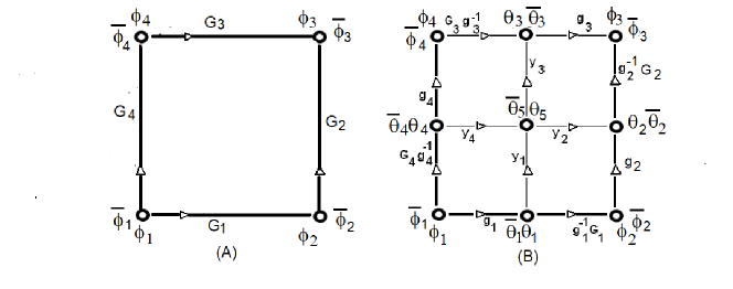
Figure 2: Subdivision of a plaquette with fermion fields

$$I = \int\mu^{\prime}\left(\overline{\phi}_{1}g_{1}\theta_{1}\overline{\theta}_{1}y_{1}\theta_{5}\left(\overline{\theta}_{4}y_{4}\theta_{5}\right)^{-1}\left(\overline{\phi}_{1}G_{4}g_{4}^{-1}\theta_{4}\right)^{-1}\right)\mu^{\prime}\left(\overline{\theta}_{1}g_{1}^{-1}G_{1}\phi_{2}\overline{\phi}_{2}g_{2}\theta_{2}\left(\overline{\theta}_{5}y_{2}\theta_{2}\right)^{-1}\left(\overline{\theta}_{1}y_{1}\theta_{5}\right)^{-1}\right)$$ (43)

$$\times\mu^{\prime}\left(\overline{\theta}_{4}y_{4}\theta_{5}\overline{\theta}_{5}y_{3}\theta_{3}\left(\overline{\phi}_{4}G_{3}g_{3}^{-1}\theta_{3}\right)^{-1}\left(\overline{\theta}_{4}g_{4}\phi_{4}\right)^{-1}\right)\mu^{\prime}\left(\overline{\theta}_{5}y_{2}\theta_{2}\overline{\theta}_{2}g_{2}^{-1}G_{2}\phi_{3}\left(\overline{\theta}_{3}g_{3}\phi_{3}\right)^{-1}\left(\overline{\theta}_{5}y_{3}\theta_{3}\right)^{-1}\right)$$

$$\times\prod_{i=1}^{5}d\mu_{H}\left(\overline{\theta}_{i}\right)d\mu_{H}\left(\theta_{i}\right)\prod_{j=1}^{4}d\mu_{H}\left(g_{j}\right)d\mu_{H}\left(y_{j}\right)$$

Let

$$g_{1}\theta_{1}\overline{\theta}_{1}y_{1}\theta_{5}=Y_{1};\;g_{2}\theta_{2}\overline{\theta}_{2}y_{2}^{-1}\theta_{5}=Y_{2};\;\overline{\theta}_{5}y_{3}\theta_{3}\overline{\theta}_{3}g_{3}=Y_{3}^{-1};\;\overline{\theta}_{5}y_{4}^{-1}\theta_{4}\overline{\theta}_{4}g_{4}=Y_{4}^{-1}$$ (44)

Then using centrality, invariance of the Haar measure and integrating over the remaining variables

$$I = \int\mu^{\prime}\left(\overline{\phi}_{1}Y_{1}Y_{4}^{-1}G_{4}^{-1}\phi_{1}\right)\mu^{\prime}\left(Y_{1}^{-1}G_{1}\phi_{2}\overline{\phi}_{2}Y_{2}\right)\mu^{\prime}\left(Y_{4}Y_{3}^{-1}G_{3}^{-1}\phi_{4}\overline{\phi}_{4}\right)\mu^{\prime}\left(Y_{2}^{-1}G_{2}\phi_{3}\overline{\phi}_{3}Y_{3}\right)$$

$$\times\prod_{i}^{4}d\mu_{H}\left(Y_{i}\right)$$

If there is a family of measures $\mu^{\prime}$, $\mu^{\prime\prime}$ and $\mu^{\prime\prime\prime}$ satisfying the semigroup property as discussed before (Eq.(19))

$$I = \int\mu^{\prime\prime}\left(Y_{4}^{-1}G_{4}^{-1}\phi_{1}\overline{\phi}_{1}G_{1}\phi_{2}\overline{\phi}_{2}Y_{2}\right)\mu^{\prime\prime}\left(G_{3}^{-1}\phi_{4}\overline{\phi}_{4}Y_{4}Y_{2}^{-1}G_{2}\phi_{3}\overline{\phi}_{3}\right)d\mu_{H}\left(Y_{2}\right)d\mu_{H}\left(Y_{4}\right)$$ (45)

$$= \int\mu^{\prime\prime}\left(G_{4}^{-1}\phi_{1}\overline{\phi}_{1}G_{1}\phi_{2}\overline{\phi}_{2}Y_{2}Y_{4}^{-1}\right)\mu^{\prime\prime}\left(Y_{4}Y_{2}^{-1}G_{2}\phi_{3}\overline{\phi}_{3}G_{3}^{-1}\phi_{4}\overline{\phi}_{4}\right)d\mu_{H}\left(Y_{2}\right)d\mu_{H}\left(Y_{4}\right)$$

$$= \mu\left(G_{4}^{-1}\phi_{1}\overline{\phi}_{1}G_{1}\phi_{2}\overline{\phi}_{2}G_{2}\phi_{3}\overline{\phi}_{3}G_{3}^{-1}\phi_{4}\overline{\phi}_{4}\right)$$

Hence the consistency condition on the measures may also be fulfilled with fermions on the lattice, by using central measures with the semigroup property. The consistency condition was verified after integration over the Grassman variables. The full measure in (41) is implicitly defined as the measure that by integration over the Grassman part of the fermion variables leads to (42).

So far, in the derivation leading to the consistency condition in Eq.(45), $G_{i},g_{i},y_{i},\phi_{i},\overline{\phi}_{i},\theta_{i},\overline{\theta}_{i}$ have been considered arbitrary group elements. However specification of a physical theory requires the choice of particular representations for these group elements. In $SU\left(n\right)$ non Abelian gauge theories is usual to choose the defining $n^{2}-1$ dimensional representation for the group elements associated to the edges of the lattice. Then to the group elements $\phi_{i},\overline{\phi}_{i},\theta_{i},\overline{\theta}_{i}$ at the vertices one may associate the fundamental $n$ and $\overline{n}$ representations. These elements always appear in the measure in the $\phi_{i}\overline{\phi}_{i}$ and $\theta_{i}\overline{\theta}_{i}$ combinations which will decompose into a scalar and a $n^{2}-1$ dimensional representation. Hence the same measure may contain both the pure gauge part and the matter fields.

5 Strata and the lattice potential

The measures, that have been discussed before, provide the probability of each particular group configuration in the lattice. In particular they provide the integration measure that controls the fluctuations around the ground state. Let us parametrize the group elements in the usual way

$$U_{\mu}\left(x\right)=e^{\int_{x}^{x+\widehat{\mu}}ds\tau_{a}A_{a}^{\mu}\left(s\right)}$$ (46)

Of particular interest are ground state configurations corresponding to condensates. Invariance of the measure implies that the fluctuations are around zero mean,

$$\left\langle A_{a}^{\mu}\right\rangle=\left\langle F_{a}^{\mu\nu}\right\rangle=0$$ (47)

$F_{a}^{\mu\nu}$ being the plaquette field, while quantities like $\left\langle A_{a}^{\mu}A_{a\mu}\right\rangle$ and $\left\langle F_{a}^{\mu\nu}F_{a\mu\nu}\right\rangle$ may be different from zero.

The multiplicity of backgrounds may be related to the strata of the gauge group operating in the lattice. The configuration space of a pure gauge lattice $L_{i}$ (associated to the group $G$) in the projective family $\mathcal{L}$ is

$$\mathcal{M=}G^{\otimes N}$$ (48)

$N$ being the number of edges in the lattice. On $\mathcal{M}$ acts the gauge group

$$\mathcal{G=}G^{\otimes N_{0}}$$ (49)

$N_{0}$ being the number of vertices in the lattice. The action of the group may be reduced from $G^{\otimes N_{0}}$ to $G$ by choosing a maximal tree gauge [27], connecting a particular vertex $x_{0}$ to all vertices in the lattice and assigning to the identity all group elements in the edges along the tree. The remaining edges not in the  tree have both vertices group-identified (more precisely, parallel transported) to the point $x_{0}$. Therefore the reduced system becomes

$$\mathcal{M}^{\prime}\mathcal{=}G^{\otimes M}$$ (50)

where in general $M<<N$ and in $\mathcal{M}^{\prime}$ acts the $G$ group by the conjugate action

$$\left(g_{1},g_{2},\cdots,g_{M}\right)\rightarrow\left(gg_{1}g^{-1},gg_{2}g^{-1},\cdots,gg_{M}g^{-1}\right)$$ (51)

$g\in G$. $\mathcal{M}^{\prime}$ is effectively a set of $M$ $\ x_{0}-$ based loops acted upon by $G$

The strata of the lattice configuration space are the strata of the action of $G$ on $G^{M}$. They are at most as many as the number of Howe subgroups of $G$ and for $G=SU\left(n\right)$ they were fully characterized by the authors of refs. [27] [28].

Let, for example, $G=SU\left(3\right)$. Let each orbit be characterized by the pair $\left(\lambda_{1},\lambda_{2}\right)$ of eigenvalues of the group elements (the two independent diagonal elements of the maximal torus) and $M\geq 2$. If the set $\left(g_{1},g_{2},\cdots,g_{M}\right)$ has no common eigenspace the stabilizer subgroup is the center of $SU\left(3\right)$ and this is the generic stratum. If there is one common eigenspace the stabilizer is $U\left(1\right)$. If there are three different common one-dimensional eigenspaces the stabilizer is $U\left(1\right)\times U\left(1\right)$ and if there is one common two-dimensional eigenspace the stabilizer is $U\left(2\right)$. Finally if there is a common three-dimensional eigenspace, meaning that all elements in $\left(g_{1},g_{2},\cdots,g_{M}\right)$ are the identity the stabilizer is $SU\left(3\right)$. Hence there are $5$ different strata.

Classical dynamics in the lattice takes place in the phase space, the cotangent bundle $T\mathcal{M}^{\prime\ast}=TG^{\otimes M\ast}$. If the initial condition lies in an orbit of a particular stratum, the classical system remains there for all its undisturbed classical evolution. Therefore for classical dynamics it makes sense to consider and classify dynamics in the different strata although, for random initial conditions, the generic strata will be almost surely chosen.

However for quantum mechanics, the situation is different because the wave function will surely explore different strata and, the generic stratum having full measure, it would seem that it is only the generic stratum that matters. Nevertheless, some authors [4] [5] have argued that in systems with gauge symmetry, where the configuration space is a orbifold with singularities corresponding to points of non-generic higher symmetry, one may find concentrations of the wave functions near the non-generic strata. This may depend on the form of the Hamiltonian used in the Schrödinger equation.

The role of the non-generic strata in the Hamiltonian formulation of the lattice theory may be analyzed with the Hamiltonian (31) and the potential (30). Let for definiteness $G=SU\left(3\right)$. The heat kernel that enters the potential (30) is a function of the two angles $\left(\theta_{1},\theta_{2}\right)$ in the maximal torus $diag\left\{\exp\left(i\theta_{1}\right),\exp\left(i\theta_{2}\right),\exp\left(-i\left(\theta_{1}+\theta_{2}\right)\right)\right\}$ of the group element associated to each plaquette. When the lattice is refined to small lattice spacing the heat kernel becomes [17]

$$K\left(\beta_{s}\right)\underset{\beta_{s}\rightarrow 0}{\longrightarrow}\exp\left\{-\frac{1}{2\beta_{s}}\left(\theta_{1}^{2}+\theta_{2}^{2}+\theta_{1}\theta_{2}\right)\right\}$$ (52)

that is, it contributes to the potential an harmonic term $\frac{1}{4\beta_{t}\beta_{s}}\left(\theta_{1}^{2}+\theta_{2}^{2}+\theta_{1}\theta_{2}\right)$.

Consider now a spatial lattice of dimension $N\times N\times N$. A maximal tree gauge starting for an upper corner is essentially equivalent to an axial gauge $A_{3}=0$ $\left(U_{3}=1\right)$. There are then $2\times N^{3}$ independent edge group elements, and $3\times N^{3}$ plaquette group elements, not all independent. Of these there are $2\times N^{3}$ plaquettes along the $3$ direction with two non-trivial edges each and $N^{3}$ plaquettes along the $1,2$ planes with four nontrivial edges.

After the gauge fixing each edge group element is still acted upon by the conjugate action as in (51) and the classification of the strata is as described before. Consider now the non-generic stratum with stabilizer $U\left(1\right)$. With a common eigenvalue in all independent links one obtains $\theta_{1}=0$ for all the plaquettes. Therefore for each fixed $\left\{\theta_{2}^{(ij)}\right\}$ configuration one obtains a minimum of the potential on this stratum. Likewise, in the strata with $SU\left(2\right)$ stabilizer one obtains $\theta_{1}=\theta_{2}=0$ for the plaquettes, another potential minimum. Hence, in the potential of this high dimensional Schrödinger problem there are multiple different local minima associated to the non-generic strata. It is intriguing to realize that this multiple minima situation is the one that might lead to a fast growing point spectrum for the gauge backgrounds, as shown in [29] using an inverse scattering argument.

References

• [1] R. Vilela Mendes; Deformations, stable theories and fundamental constants, J. Phys.A Math. Gen. 27 (1994) 8091-8104.
• [2] R. Vilela Mendes; Geometry, stochastic calculus, and quantum fields in a noncommutative space–time, J. Math. Phys. 41 (2000) 156-186.
• [3] R. Vilela Mendes; Commutative or noncommutative spacetime? Two length scales of noncommutativity, Physical Review D 99 (2019) 123006.
• [4] B. De Barros Cobra Damgaard and H. RΓΆmer; Quantum Gravity and SchrΓΆdinger Equations on Orbifolds, Letters in Mathematical Physics 13 (1987) 189-193.
• [5] C. Emmrich and H. RΓΆmer; Orbifolds as Configuration Spaces of Systems with Gauge Symmetries, Commun. Math. Phys. 129 (1990) 69-94.
• [6] G. Triantaphyllou; A New Paradigm for the Fermion Generations, Helvetica Physica Acta, 67 (1994)Β 660-682.
• [7] A. Blumhofer and M. Hutter; Family structure from periodic solutions of an improved gap equation; Nuclear Physics B 484 (1997) 80-96.
• [8] J. KisyΕ„ski; On the generation of tight measures, Studia Mathematica 30 (1968) 141-151.
• [9] K. Maurin; General Eigenfunction Expansions and Unitary Representations of Topological Groups, PWN - Polish Scientific Publishers, Warszawa 1968.
• [10] M. M. Rao; Stochastic Processes: General Theory, Springer, Dordrecht 1995.
• [11] J. Jorgenson and S. Lang; The ubiquitous heat kernel, in Mathematics Unlimited - 2001 and beyond, pp. 655-683, B. Engquist and W. Schmid (Eds.), Springer, Berlin 2001.
• [12] J. Jorgenson and Walling (Eds.); The Ubiquitous Heat Kernel, American Mathematical Society 2006.
• [13] K. Bogdan, P. Sztonyk and V. Knopova; Heat kernel of anisotropic nonlocal operators, arXiv:1704.03705.
• [14] L. Michel; Points critiques des fonctions invariants sur une G-variΓ©tΓ©, Comptes Rendus Acad. Sci. Paris 272-A (1971) 433–436.
• [15] G. Rudolph, M. Schmidt and I. P. Volobuev; On the gauge orbit space stratification: a review, J. Phys. A: Math. Gen. 35 (2002) R1–R50.
• [16] R. Vilela Mendes; Stratification of the orbit space in gauge theories: the role of nongeneric strata, J. Phys. A: Math. Gen. 37 (2004) 11485–11498.
• [17] R. Vilela Mendes; An infinite-dimensional calculus for generalized connections on hypercubic lattices, J. Mathematical Physics 52 (2011) 052304.
• [18] R. Vilela Mendes; A consistent measure for lattice Yang Mills, Int. J. Modern Physics A 32 (2017) 1750016.
• [19] J. M. Drouffe; Transitions and duality in gauge lattice systems, Phys. Rev. D 18 (1978) 1174-1183.
• [20] P. Menotti and E. Onofri; The action of SU(N) lattice gauge theory in terms of the heat kernel on the group manifold, Nuclear Physics B190[FS3] (1981) 288-300.
• [21] S. Klimek and W. Kondracki; A Construction of Two-Dimensional Quantum Chromodynamics, Commun. Math. Phys. 113 (1987) 389-402.
• [22] M. Creutz; Quarks, gluons and lattices, Cambridge Univ. Press, London 1983.
• [23] K. Osterwalder and E. Seiler; Gauge Field Theories on a Lattice, Annals of Physics 110 (1978) 440-471.
• [24] J. Kogut and L. Susskind; Hamiltonian formulation of Wilson’s lattice gauge theories, Phys. Rev. D 11 (1975) 395-408.
• [25] A. Henrot; Extremum problems for eigenvalues of elliptic operators, BirkhΓ€user Verlag, Berlin 2006.
• [26] L. Michel and L.Β A. Radicati; Geometry of the octet, Ann. Inst. Henri PoincarΓ© A18 (1973) 185.
• [27] S. Charzynskia, J. Kijowskia, G. Rudolph and M. Schmidt; On the stratified classical configuration space of lattice QCD, Journal of Geometry and Physics 55 (2005) 137–178.
• [28] G. Rudolph, M. Schmidt and I. P. Volobuev; Classification of Gauge Orbit Types for SU(n)-Gauge Theories, Mathematical Physics, Analysis and Geometry 5 (2002) 201–241.
• [29] R. Vilela Mendes; On potentials with fast growing point spectrum, Physics Letters B 155 (1985) 274-277.