BigDatasetGAN: Synthesizing ImageNet with Pixel-wise Annotations

Abstract

Annotating images with pixel-wise labels is a time-consuming and costly process. Recently, DatasetGAN [82] showcased a promising alternative – to synthesize a large labeled dataset via a generative adversarial network (GAN) by exploiting a small set of manually labeled, GAN-generated images. Here, we scale DatasetGAN to ImageNet scale of class diversity. We take image samples from the class-conditional generative model BigGAN [6] trained on ImageNet, and manually annotate only 5 images per class, for all 1k classes. By training an effective feature segmentation architecture on top of BigGAN, we turn BigGAN into a labeled dataset generator. We further show that VQGAN [19] can similarly serve as a dataset generator, leveraging the already annotated data. We create a new ImageNet benchmark by labeling an additional set of real images and evaluate segmentation performance in a variety of settings. Through an extensive ablation study, we show big gains in leveraging a large generated dataset to train different supervised and self-supervised backbone models on pixel-wise tasks. Furthermore, we demonstrate that using our synthesized datasets for pre-training leads to improvements over standard ImageNet pre-training on several downstream datasets, such as PASCAL-VOC, MS-COCO, Cityscapes and chest X-ray, as well as tasks (detection, segmentation). Our benchmark will be made public and maintain a leaderboard for this challenging task. Project Page: https://nv-tlabs.github.io/big-datasetgan/

1 Introduction

The ImageNet dataset [68] has served as a cornerstone of modern computer vision and deep learning. It is used as a testbed for innovating in the domain of large-scale classification, and has enabled incredible advancements over the years [44, 70, 30, 16]. Importantly, it has also been commonly used for pre-training backbone models, with either supervised or recently self-supervised pre-training, leading to almost guaranteed performance gains on a plethora of downstream datasets and tasks [25, 81]. ImageNet contains a million images with 1000-way classification labels. This huge class diversity is what makes pre-trained networks generalize well to a variety of downstream applications.

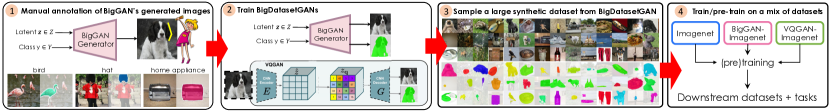
Figure 2: BigDatasetGAN overview: (1) We sample a few images per class from BigGAN and manually annotate them with masks. (2) We train a feature interpreter branch on top of BigGAN’s and VQGAN’s features on this data, turning these GANs into generators of labeled data. (3) We sample large synthetic datasets from BigGAN & VQGAN. (4) We use these datasets for training segmentation models.

In this paper, we aim to enhance ImageNet with pixel-wise labels, to enable large-scale multi-class segmentation challenges and offer opportunities for new pre-training strategies for dense downstream prediction tasks. However, instead of manually labeling masks for 1M images, which is time-consuming and costly, we instead synthesize high quality labeled data at a fraction of the cost.

We build on top of DatasetGAN [82], which introduced a simple idea: to manually annotate a very small set of GAN-generated images with pixel-wise labels, and add a shallow segmentation branch on top of the GAN’s feature maps which is trained on this small dataset. It was shown that the generator’s feature maps are incredibly powerful and semantically meaningful, and allow the segmentation branch to produce very accurate labels for new random samples from the GAN. This means that the GAN is successfully re-purposed into a dataset generator, producing samples in the form of images and their pixel-wise labels. The authors showed that synthesizing a large dataset and using it to train downstream segmentation networks leads to extremely high performance at only a fraction of the labeling cost. However, DatasetGAN utilized StyleGAN [39] as the generative model, which is limited to single class modeling.

In this paper, we scale DatasetGAN to the ImageNet scale, propose a novel pixel-wise ImageNet benchmark, and perform an extensive analysis of several existing methods on this benchmark. Specifically, we adopt the class-conditional generative model BigGAN [6], which has been shown to produce high quality image samples for the 1k ImageNet classes. By manually labeling a handful of sampled images per class using a single expert annotator to ensure consistency and accuracy, we are able to synthesize a high quality labeled synthetic dataset. We further show that VQGAN [19] can also serve as a dataset generator without the need for an additional annotation effort. We call a dataset generator for ImageNet obtained like that BigDatasetGAN. We show the benefits of leveraging synthesized datasets for a plethora of downstream dense prediction tasks and datasets. We demonstrate significant performance gains on PASCAL-VOC, MS-COCO, Cityscapes and chest X-ray for tasks such as object detection and instance segmentation, leveraging several different backbone models. Furthermore, we annotate a held-out subset of real ImageNet with pixel-wise labels and introduce a new semantic segmentation benchmark. We compare several supervised and self-supervised methods and show that when these utilize our synthetic datasets their performance is significantly improved. Our benchmark will be hosted online, maintaining a leaderboard for a suite of segmentation challenges.

2 Related Work

Reducing Annotation Cost

Reducing labeling costs can be achieved in a variety of ways, such as interactive human-in-the-loop annotation [67, 2, 56, 77, 53], nearest-neighbor mask transfer [54, 73, 66, 27], or using weak supervision in the form of cheaper labels such as object boxes [8, 45, 47], scribbles [50, 72] or very coarse masks [1]. A full review is out of scope of this paper. Most related to our goal are the existing efforts to label ImageNet with pixel-wise annotations. In [27], the authors label 10 images per class, for 500 ImageNet classes, and iteratively propagate these labels to other images. At each stage, they perform segmentation transfer to the most similar images, and define various potentials in a graphical model to derive the final segmentation. While they show promising segmentation propagation performance, they do not showcase the usefulness of the auto-labeled dataset, as we do in our work. Here, we also leverage modern deep learning techniques, GANs in particular, likely leading to higher quality datasets.

Synthetic Dataset Generation

The labeling cost can also be alleviated by relying on 3D graphics engines that render images along with perfect annotations. Several synthetic datasets with rich labels have been created in this way [59, 61, 23, 65, 64, 17]. However, these datasets typically exhibit a domain gap with respect to real-world datasets in terms of both appearance as well as content. A variety of methods translate the rendered images into more realistic ones using GAN-based techniques [33] to close the appearance gap. Recent works also propose to learn the parameters of the data generation pipeline to reduce the distribution gap [37, 15, 48]. Moreover, creating ImageNet-level of class and instance diversity via the graphics approach would require significant 3D content acquistion efforts.

Generative models of images can be considered as a neural rendering alternative to graphics engines. High fidelity images can now be generated by unconditional GANs such as StyleGAN [39, 40, 38], typically for a single class. Class-conditional generative models such as BigGAN [6] and VQGAN [19] have shown impressive modeling capabilities across multiple classes. The recent DatasetGAN [82] and similar methods [80] showed strong performance on pixel-wise segmentation when utilizing GANs to synthesize labeled data, requiring only a handful of GAN-generated images to be manually labeled. Works like [49, 24, 74] use an encoder to embed real images into a GAN’s latent space and train a segmentation branch on top of the GAN’s features to produce pixel-wise labeling of real images. These works mostly operate in a single-class regime, with an unconditional generative model like StyleGAN as backbone. In our work, we scale these ideas to the ImageNet scale, leveraging conditional generative models BigGAN and VQGAN, and provide extensive analysis in this setting.

Representation Learning

Pre-training followed by finetuning is an effective paradigm in training neural networks. Supervised classification pre-training on large-scale datasets such as ImageNet affords large performance boosts when fine-tuning on domain-specific tasks [25, 81]. Recently, self-supervised approaches such as contrastive learning (CL) [10, 11, 76, 60, 79] have become a widely used alternative to supervised pre-training. These methods do not require any labels, and in some cases lead to higher gains on dense downstream tasks than supervised pre-training [76]. Our effort here is complementary to this line of work, and we analyze the effectiveness of these methods when combined with our synthesized datasets.

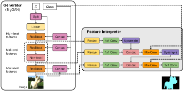
Figure 3: Architecture of BigDatasetGAN based on BigGAN [6].

3 BigDatasetGAN

We extend DatasetGAN [82] to synthesize ImageNet images with pixel-wise labels. In particular, we utilize the two ImageNet-pretrained conditional generative models BigGAN [6] and VQGAN [19], and enhance each with a segmentation branch, called a feature interpreter (Sec. 3.1). We choose these two models mainly as they represent widely-used and high-performance conditional generative models of images. We also wish to compare them since their architectures and training approaches are largely different: BigGAN has a fully convolutional architecture and is trained purely via standard adversarial objectives. VQGAN uses convolutional encoder and decoder networks, and also utilizes an autoregressive transformer on top of compressed and vector-quantized images in latent space.

We draw a handful of samples from BigGAN and manually label them with pixel-wise annotations, a procedure which we describe in Sec. 4. We choose to label BigGAN’s samples instead of VQGAN’s for a pragmatic reason: We find that VQGAN is able to embed real images (and BigGAN’s samples) with excellent reconstruction fidelity, and thus enables us to leverage annotated BigGAN samples. In contrast, no satisfactory encoders for BigGAN exist to date. Using the annotated BigGAN images, we then train feature interpreter branches to predict pixel-wise segmentation labels for both BigGAN and VQGAN, following a similar approach as the original DatasetGAN [82]. Finally, we synthesize two large datasets by drawing labeled samples from both BigGAN and VQGAN, using filtering steps to ensure high quality of the final datasets, as described in Sec. 3.2.

3.1 Generative Models of Datasets

Generative models learn a distribution over data, e.g., images. In the GAN framework, a generative model $\mathcal{G}$ is a function that maps latent variables $\mathbf{z}$, usually drawn from a Normal distribution $\mathbf{z}\sim\mathcal{N}(\mathbf{z};\mathbf{0},\textbf{I})$, to an image $\mathbf{x}$. Conditional GANs [6] include class information $y^{c}$ as input to the generator $\mathcal{G}(\mathbf{z},y^{c})$. The generator $\mathcal{G}$ is often a convolutional neural network with sub functions $g_{i}$ that operate at increasingly higher spatial resolutions. We can formally write $\mathcal{G}(\mathbf{z},y^{c})=g_{l-1}\circ g_{l-2}\circ\cdots\circ g_{0}(\mathbf{z},y^{c})$, where $l$ is the number of layers. If we define intermediate features $\mathbf{f}_{i}$ as the output of $g_{i}$, we obtain the set of GAN features $F_{\mathcal{G}}=\{\mathbf{f}_{0},\mathbf{f}_{1},\cdots,\mathbf{f}_{l-1}\}$ from the outputs of all the intermediate layers of $\mathcal{G}$.

We wish to learn a feature interpreter function $\mathcal{S}(F_{\mathcal{G}},y^{c})\rightarrow\mathbf{y}^{d}$ that takes a generator’s features $F_{\mathcal{G}}$ and a class label $y^{c}$ as input and outputs the set of all pixel-wise labels $\mathbf{y}^{d}$ for that class. $\mathcal{G}$ and $\mathcal{S}$ can be used together to generate a densely annotated dataset. We next discuss two different architectures, BigGAN and VQGAN, and introduce our feature interpreters’ architectures on top of them.

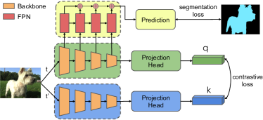
Figure 4: Simple architecture for adding a supervised segmentation branch to self-supervised representation learners.

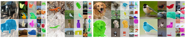
(a) Real-annotated

(b) Synthetic-annotated

(c) BigGAN-sim

(d) VQGAN-sim

Figure 5: Examples from our datasets: Real-annotated (real ImageNet subset labeled manually), Synthetic-annotated (BigGAN’s samples labeled manually), and synthetic BigGAN-sim, VQGAN-sim datasets. Notice the high quality of synthetic sampled labeled examples.

Figure 6: Mean shapes from our BigGAN-sim dataset. For our 100k BigGAN-sim dataset, each class has around 100 samples. We crop the mask from the segmentation label and run k-means with 5 clusters to extract the major modes of the selected ImageNet class shapes.

	Dataset Statistics					Image Quality		Label Quality		Geometry Analysis
Dataset	Size	IN	MI	BI	MB	FID $\downarrow$	KID $\downarrow$	FID $\downarrow$	KID $\downarrow$	PL	SC	SD
Real-annotated	8k	1.91	0.315	0.501	0.581	0.0	0.0	0.0	0.0	3.89	34.4	7.98
Synthetic-annotated	5k	1.15	0.314	0.449	0.665	17.91	1.84	20.69	6.33	3.77	28.1	6.13
BigGAN-sim	100k	1.33	0.261	0.403	0.606	19.45	3.47	44.88	25.22	3.65	33.9	6.67
VQGAN-sim	100k	1.52	0.375	0.615	0.583	21.21	11.10	48.55	33.28	3.81	30.8	5.13

Table 1: Dataset analysis. We report image & mask statistics across our datasets (naming explained in Fig. 5). We compute image and label quality using FID and KID and use Real-annotated dataset as reference. IN: instance count per image, MI: ratio of mask area over image area, BI: ratio of tight bounding box of the mask over image area, MB: ratio of mask area over area of its tight bounding box, PL: polygon length (polygon normalized to width and height of 1), SC: shape complexity measured by the number of points in a simplified polygon, SD: shape diversity measured by mean pair-wise Chamfer distance [22] per class and averaged across classes.

BigGAN

BigGAN [6] adopts a convolutional architecture, illustrated in Fig. 3 on the left-hand side. Given random noise $\mathbf{z}$ and a class label $y^{c}$, we obtain BigGAN’s generator features $F_{\textrm{BigGAN}}$ from different layers. We group features from different spatial resolutions into high-, mid- and low-level by their semantic meaning. Specifically, we group the first three ResBlocks into a high-level group with resolutions $8\times 8$ to $32\times 32$. We group the next three ResBlocks including one attention block together as a mid-level group with resolutions from $64\times 64$ to $128\times 128$. The last two ResBlocks before the image output layer are grouped into a low-level group with resolutions $256\times 256$ to $512\times 512$. Note that high-level features in lower layers have a very high feature dimensionality, i.e., $1536\times 8\times 8$.

DatasetGAN [82] resizes all features into the final resolution, resulting in a large memory cost. Due to the high memory consumption, they need to randomly sample pixel-wise features when learning the MLP-based interpreter, rather than using the entire feature map. We propose to first resize features in the same group into the highest resolution within the group, and then use 1x1conv to reduce feature dimensionality before upsampling all the features to the resolution in the next level. After upsample, features from lower layers are concatenated with the resized features from the current level following the same operations as described above. Features from two levels are then fused by a mix-conv operation which includes two 3x3conv operations with a residual connection and a conditional batchnorm operation with class information, similar to [6]. The same process is repeated in the low-level group, and a final 1x1conv is used to output the segmentation logits. Compared to DatasetGAN, this design greatly reduces the memory cost and can use contextual information in the mix-conv operation (see Fig. 3).

VQGAN

One notable difference between BigGAN and VQGAN [19] is that VQGAN incorporates an encoder that maps real images into a discrete latent space. In contrast to BigGAN, this ability allows VQGAN to exploit a labeled dataset of images that does not necessarily come from VQGAN sampling itself. In addition to the encoder, VQGAN has a learned class-conditional autoregressive transformer network that operates on the discrete indices of the output of the encoder. Specifically, this transformer is used to learn the discrete latent space distribution and allows a user to sample novel images from the model. A convolutional decoder is used on top of the discrete tokens to produce an image. For our feature interpreter, we found it to be critical to use the features of the transformer as they contain semantic knowledge about the input image. Specifically, we gather features from every fourth transormer layer for each spatial location $(16\times 16)$ of the encoder output. We also use all decoder feature layers. Combining everything yields the set of features $F_{\textrm{VQGAN}}$. We then follow the architecture design as for BigGAN to obtain output segmentation maps.

3.2 Synthesizing Labeled Data

We sample large datasets from BigGAN and VQGAN by using several filtering steps to ensure high quality of the synthesized images and their labels. Examples are shown in Fig. 5, with the dataset analysis provided in Sec. 5.1.

Filtering

For BigGAN, we use the Truncation Trick[6] where the noise $\mathbf{z}$ is sampled from a truncated Normal with truncation value $0.9$ to reduce noisy samples. Although lower truncation values will increase overall image fidelity and label quality as the samples are closer to the major modes of the data distribution, sample diversity is also important for downstream task performance. We further use rejection sampling [62], where a pre-trained image classifier is used to rank the samples by their confidence scores, to achieve finer control over the trade-off between sample diversity and quality. We use a rejection rate of $0.9$ in our experiments. Since only 5 images on average are annotated for each class, the segmentation branch is likely to overfit. In order to alleviate this issue, we follow [82] to train an ensemble model of 16 segmentation heads and use the Jensen-Shannon divergence as uncertainty measure to filter out the top 10% most uncertain images [57, 4, 46]. For VQGAN, we use top-200 filtering and nucleus sampling [32] with $p=0.92$ which samples from the top-$p$ portion of the probability mass, using only the top 200 out of 16k indices.

Offline vs Online Sampling

Synthesizing a static dataset incurs a one-time computational cost, and allows us to compare different segmentation methods on the same dataset. We also explore an online strategy, where our BigDatasetGAN is used to synthesize data online during training of a downstream segmentation model. This exposes the model to a much greater variety of data, as it never sees the same labeled examples twice during training. In our experiments, this strategy improves task performance by 1-2% for our ImageNet segmentation benchmark over using a static 100k-sized, sampled dataset. Compared to offline sampling, training with online sampling converges faster, as observed previously [58]. However, it is slower, as in each training iteration the generative model needs to be run. Therefore, we explore this approach only with the BigGAN-based model, as VQGAN sampling is particularly slow due to its autoregressive transformer component. Furthermore, we also drop expensive filtering methods like using an ensemble model in the interest of computational efficiency when performing online sampling. We provide an analysis of the online sampling strategy for one selected method in Tab. 2, denoted with BigGAN-off (offline generated dataset) and BigGAN-on (online sampling).Whenever not explicitly mentioned, our experiments use the offline sampling strategy.

4 Annotating ImageNet with Pixel-wise Labels

The first important choice to consider is what data to label manually to form the training set for our feature interpreters. While the GANs ensure that we can operate in the low-label regime, labeling all 1k ImageNet classes still incurs a cost, mainly in labeling time as we utilize a single annotator. Since BigGAN does not have the ability to encode images and thus utilize any labeled data – in contrast to VQGAN, which has an encoder – we opt to label BigGAN’s samples. Note that BigGAN’s samples are mostly very realistic and diverse. We highlight that BigGAN produces samples 150 times faster than VQGAN, and is thus more convenient for more massive-scale experiments.

From each category, we randomly selected 10 images for annotation from both the ImageNet, and BigGAN generated images. For each of the 1k categories, a single annotator segmented both the real and synthetic images. Both sets were annotated consecutively starting with the real images and then segmenting the BigGAN images to facilitate the recognition of the synthetic images. The annotator labeled 5 images per class and dataset on average, ignoring low quality images with unrecognizable objects. Out of the 1k categories, only for 3 categories the annotator could not identify any of the images generated by BigGAN.

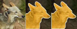
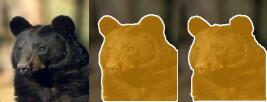
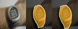
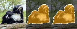
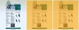
red wolf: 97.7/ 0.8	black bear: 97.5/ 1.0	watch: 95.8/ 1.0	terrier: 95.6/ 1.0	website: 95.4/ 1.0
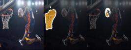
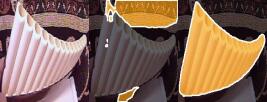
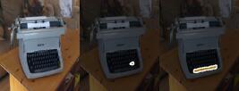
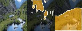
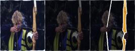
basketball: 0.1/1.0	pandean pipe: 1.8/1.0	space bar: 2.4/0.7	valley: 2.5/0.5	bow: 3.9/1.0

Figure 7: Top-5 analysis of ImageNet benchmark. Text below images indicates: Class name, FG/BG segmentation measured in mIoU, classification accuracy of a Resnet-50 pre-trained on ImageNet. Top Row: We visualize Top-5 best predictions of DeepLabv3 trained on BigGAN-sim dataset for the FG/BG task, compared to ground-truth annotations (third column). Bottom Row: We visualize Top-5 worst predictions. Typical failure cases include small objects or thin structures. Interestingly, classes the are hard to segment, such as baskeball and bow, are not necessarily hard to classify.

	Method	Dog	Bird	FG/BG	MC-16	MC-100	MC-128	MC-992	Mean
superv. pre-train.	Rand	56.4	35.7	44.7	13.9	4.0	3.6	2.3	22.9
2-10	Sup.IN	82.6	79.6	66.3	58.7	56.1	28.5	17.8	55.7
	+ BigGAN-off	85.8	81.2	67.5	64.6	62.3	29.3	22.8	59.0
	+ BigGAN-on	87.0	83.2	69.5	66.1	62.8	29.5	24.6	60.4
2-10	SupCon [41]	83.8	79.0	66.6	59.2	55.4	28.6	18.7	55.9
	SupSelfCon [35]	84.4	81.8	67.6	63.1	60.0	28.3	18.9	57.8
	+ BigGAN-sim	87.0	83.2	69.5	66.1	62.8	32.8	29.7	61.6
	+ VQGAN-sim	86.7	84.4	71.1	68.1	64.7	30.4	25.8	61.6
self-superv. pre-train.	SimCLR[10]	77.7	73.7	66.7	53.8	44.3	29.3	16.0	51.6
	MoCo-v2[11]	84.6	82.7	65.6	51.4	39.1	18.5	10.2	50.3
	BYOL[26]	78.0	72.9	68.5	55.4	45.8	27.7	16.1	52.1
	DINO[7]	77.8	72.7	66.1	50.5	41.2	23.2	12.7	49.2
2-10	DenseCL[76]	85.0	83.3	62.5	47.9	38.6	17.3	13.1	49.7
	+ BigGAN-sim	86.5	84.9	66.4	58.6	41.0	17.9	19.9	53.6
	+ VQGAN-sim	86.7	85.9	67.1	59.3	41.7	19.3	16.8	53.8
2-10	MoCo-v3[12]	77.2	71.5	67.4	54.0	49.7	30.1	17.4	52.5
	+ BigGAN-sim	83.3	76.7	71.1	64.8	58.1	38.9	30.8	60.5
	+ VQGAN-sim	83.8	80.9	71.7	66.5	61.2	41.5	33.5	62.7

Table 2: ImageNet pixel-wise benchmark. We compare various methods on several tasks, with supervised and self-supervised pre-training. We use Resnet-50 for all methods. We ablate the use of synthetic datasets for three methods. FG/BG evaluates binary segmentation across all classes; MC-N columns evaluate multi-class segmentation performance in setups with $N$ classes. Adding synthetic datasets improves performance by a large margin BigGAN-off and BigGAN-on compare offline & online sampling strategy.

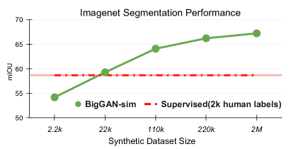
Figure 8: Ablating synthetic dataset size. Here we fix the model to the Resnet50 backbone and compare the performance when we increase the synthetic dataset size. The model trained using a 22k synthetic dataset outperforms the same model trained with 2k human-annotated dataset. Another 7 points is gained when further increasing the synthetic data size from 22k to 220k. Here, 2M is the total number of samples synthesized through our online sampling strategy (See Sec. 3.2).

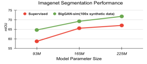
Figure 9: Ablating backbone size. We scale up the backbone from Resnet50 to Resnet101 and Resnet152. We supervise with 2k human-annotated labels (red), and with our BigGAN-sim dataset (green), which is 100x larger. BigGAN-sim dataset supervision leads to consistent improvements, especially for larger models.

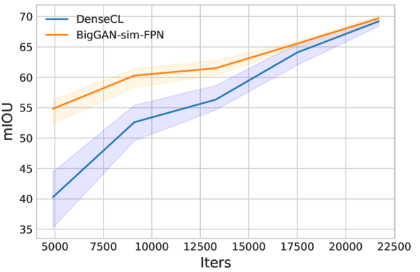
Figure 10: Convergence of segm. performance on Pascal-VOC. We evaluate val. set semantic segmentation at different training iterations. Backbone pre-trained using our synthetic dataset shows significantly faster convergence rates compared to training with contrastive learning alone. Colored area indicates variance over 5 trials.

5 Analysis and Experiments

In Sec. 5.1, we provide analyses of our synthesized datasets compared to the real annotated ImageNet samples and highlight new insights into ImageNet through segmentation. In Sec. 5.2, we evaluate several state-of-the-art supervised and self-supervised representation learning methods by competing on our (real) pixel-wise ImageNet benchmark and ablate the use of our synthetic datasets. Finally, in Sec. 5.3 we showcase the benefits of our synthesized data for pre-training of downstream models on various datasets. Further experiment details and analyses in Supp. Material.

5.1 Dataset Analysis

We first study our four different datasets in Table 1: (1) Real manually annotated dataset (size 8k), which is used as benchmark testing data. (2) Synthetic manually annotated BigGAN dataset (size 5k), which is used as benchmark training data. And two synthetic datasets (3) BigGAN-sim (size 100k) and (4) VQGAN-sim (size 100k) generated from BigGAN and VQGAN, respectively. We compare image and label quality in terms of distribution metrics using the real annotated dataset as reference. We also compare various label statistics and perform shape analysis on labeled polygons in terms of shape complexity and diversity.

Synthetic vs. real dataset

Compared to the Real-annotated dataset, the Synthetic-annotated dataset shows a distribution gap in terms of FID/KID [31, 5] on sampled images masked by segmentation labels (Table 1, also see Fig. 5 and Fig. 6). We compute metrics on masked images to avoid noisy backgrounds. Among the synthetic datasets, BigGAN-sim has better image and label quality in terms of FID/KID compared to VQGAN-sim ($19.45/3.47$ vs. $21.21/11.10$). However, VQGAN-sim contains on average 1.52 instances per image (IN) compared to BigGAN-sim (1.33). This indicates that VQGAN can better model multiple objects in individual images. Interestingly, BigGAN-sim labels have a higher Shape Complexity (SC) score compared to VQGAN-sim ($33.9$ vs. $30.8$) measured by the average number of points in polygons simplified by the Douglas-Peucker algorithm [18] with threshold 0.01. The Shape Diversity (SD) metric is also slightly better for BigGAN. Note that we may be seeing some of the effects of training VQGAN on BigGAN’s data.

5.2 ImageNet Segmentation Benchmark

We introduce a benchmark with a suite of segmentation challenges using our Synthetic-annotated dataset (5k) as training set and evaluate on our Real-annotated held-out dataset (8k); please refer to Table 1 for details. Specifically, we evaluate performance for (1) two individual classes (dog and bird), (2) foreground/background (FG/BG) segmentation evaluated across all 1k classes, and (3) multi-class semantic segmentation for various subsets of classes.

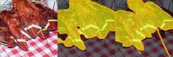
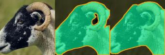
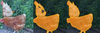
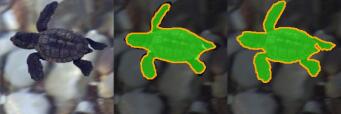
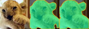
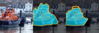
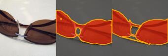
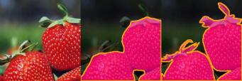
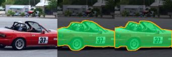
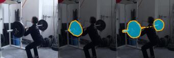
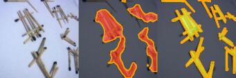
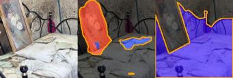
Figure 11: Qualitative results on MC-128. We visualize predictions (second column) of DeepLab trained on our BigGAN-sim dataset, compared to ground-truth annotations (third column). The final row shows typical failure cases, which include multiple parts, thin structures or complicated scenes.

Task setup

Dog and Bird evaluate binary segmentation. For Dog, we group 118 dog classes in ImageNet1k, resulting in 657 training images. For Bird, we group 59 bird classes, with 366 training images. The FG/BG task evaluates binary segmentation accuracy over all classes, while MC-16 is multi-class segmentation on a group of 16 common objects like boat, car and chair, similar to PASCAL VOC [21]. MC-100 is also multi-class segmentation over randomly selected 100 ImageNet1k classes. Task MC-128 uses top-down grouping based on WordNet [34], resulting in a long-tailed class distribution, suitable for testing class-imbalanced segmentation. MC-992 is a multi-class segmentation task on all 992 ImageNet1k classes, where we filtered out 8 classes that BigGAN cannot model well.

Evaluation

All segmentation methods we compare are based on DeepLabv3 [9] with Resnet-50 [30]. The evaluation metric is mean Intersection-over-Union (mIoU).

Comparisons

In Table 2, we compare state-of-the-art self-supervised learning (SSL) methods based on either contrastive learning or knowledge distillation. We also compare performance over supervised pre-training on ImageNet. Since SSL methods do not use class information, we also include the backbone pre-trained using Supervised Contrastive Learning (SupCon) [41] and MoCo-v2 jointly trained with classification (SupSelfCon) [35]. We observe that whenever a method is trained using our large synthetic datasets (in contrast to only using the manually labeled dataset) the task performance improves. Specifically, the MoCo-v3 pre-trained backbone trained using the VQGAN-sim dataset improves mean performance by 10.2 over the 7 tasks. In MC-16, the DenseCL [76] pre-trained backbone improves its performance by 11.4 with our synthetic dataset.

VQGAN-sim vs. BigGAN-sim

In our benchmark, VQGAN-sim and BigGAN-sim have the same dataset size of 100k labeled images. In terms of task performance, methods trained with VQGAN-sim achieve overall better performance. However, VQGAN is a massive model with 1.5B parameters including the transformer, while BigGAN has only 110M parameters. In terms of inference speed, since VQGAN samples autoregressively, it takes on average 15 sec. per image, whereas BigGAN’s inference speed is around 0.1 sec. per image. Sampling a 2M synthetic dataset would take almost an entire year for VQGAN vs. 55 hours for BigGAN on a single GPU. As discussed, this also makes it impractical to use the online sampling strategy with VQGAN during training of downstream task models.

Scaling up dataset size

A useful property of generative models is the ability to synthesize large amounts of data. In Fig. 10, we show that task performance increases when scaling up dataset size. A model trained with a 22k-sized synthetic dataset from BigGAN-sim outperforms the same model trained with 2k human-annotated labels. We observe another gain of 7 points when scaling dataset size from 22k to 220k. A further but less significant boost is seen at 2M.

Scaling up model size

We also analyze the effect of the model size. In Fig. 10, we compare a baseline model trained with 2k human-annotated labels with the same model trained with the 100x larger BigGAN-sim dataset. We see large performance gains at all model sizes when leveraging our large simulated dataset.

Classification vs. segmentation

Furthermore, we study whether shapes which are difficult to segment are also hard to classify. In Table 7, we show the Top-5 worse/best classes in terms of class-wise FG/BG segmentation. We find that classes with thin structures, like bow, as well as objects with heavy occlusions and no clear boundaries, are hard to segment but not necessarily difficult to classify.

pre-train	$AP^{bb}$	$AP^{bb}_{50}$	$AP^{bb}_{75}$	$AP^{mk}$	$AP^{mk}_{50}$	$AP^{mk}_{75}$
random init.	31.0	46.8	30.4	28.5	46.8	30.4
supervised	38.9	59.6	42.7	35.4	56.5	38.1
MoCo-v2[11]	38.9	59.2	42.4	35.4	56.2	37.8
DenseCL[76]	39.4	59.9	42.7	35.6	56.7	38.2
BigGAN-sim-FPN	39.8	60.4	43.7	35.9	57.3	38.2

(a) Mask R-CNN R50-FPN, 1× schedule

pre-train	$AP^{bb}$	$AP^{bb}_{50}$	$AP^{bb}_{75}$	$AP^{mk}$	$AP^{mk}_{50}$	$AP^{mk}_{75}$
random init.	36.7	56.7	40.0	33.7	53.8	35.9
supervised	40.6	61.3	44.4	36.8	58.1	39.5
MoCo-v2[11]	40.9	61.5	44.6	37.0	58.4	39.6
DenseCL[76]	41.2	61.9	45.1	37.3	58.9	40.1
BigGAN-sim-FPN	41.5	62.2	45.4	37.5	59.0	40.5

(b) Mask R-CNN R50-FPN, 2× schedule

Table 3: MS-COCO object detection & instance segmentation. Using our synthetic data during pre-training improves object detection performance by 0.4 $AP^{bb}$, and instance segmentation by 0.3 $AP^{mk}$ in $1\times$ training schedule. When training longer in the $2\times$ schedule, our synthetic data consistently helps improving the task performance by 0.3 $AP^{bb}$ and 0.2 $AP^{mk}$.

	Detection			Semantic seg.
pre-train	$AP$	$AP_{50}$	$AP_{75}$	mIoU
random init.	33.8	60.2	33.1	40.7
supervised	53.5	81.3	58.8	67.7
MoCo-v2[11]	57.0	82.4	63.6	67.5
DenseCL[76]	58.7	82.8	65.2	69.2
BigGAN-sim-FPN	58.2	83.0	65.5	69.7

Table 4: PASCAL VOC detection & semantic segmentation. For detection, we follow [28] and train on the trainval’07+12 set and evaluate on test07. For semantic segmentation, we train on train aug2012 [49] and evaluate on val2012. Results are average over 5 individual trials.

pre-train	$1\%$	$5\%$	$10\%$	$50\%$	$100\%$
supervised	49.6	47.8	54.1	57.6	63.6
DenseCL[76]	48.8	59.4	66.2	69.2	70.4
BigGAN-sim-FPN	67.6	70.8	71.2	74.7	75.3

Table 5: Semi-supervised chest X-ray segmentation with a frozen backbone. Performance numbers are mIoU. When using our synthetic dataset, we match the performance of the supervised and self-supervised pre-trained networks with only 1% and 5% of labels, respectively. We achieve a big gain using 100% of the data. Numbers are averaged over 3 independent trials.

	Instance seg.		Semantic seg.
pre-train	$AP^{mk}$	$AP^{mk}_{50}$	mIoU
random init.	25.4	51.1	63.5
supervised	32.9	59.6	73.7
MoCo-v2[11]	33.7	61.8	74.5
DenseCL[76]	34.5	62.1	75.7
BigGAN-sim-FPN	34.8	62.9	75.6

Table 6: Cityscapes instance and semantic segmentation. We train on train_fine set and evaluate on val set.

5.3 Transfer Learning

Here, we propose a simple architecture design to jointly train model backbones with contrastive learning and supervision from our synthetic datasets (Fig.5). We conduct experiments with SSL approaches for dense prediction tasks on MS-COCO[52], PASCAL-VOC[20], Cityscapes[14], as well as chest X-ray segmentation in the medical domain.

Pre-training with synthetic data

We build on top of state-of-the-art contrastive learning method DenseCL [76], which extends MoCo-v2 [11] with a dense contrastive loss. We design a shallow semantic segmentation decoder based on feature pyramid networks (FPN), similar to [43], to train a segmentation branch on our synthetic dataset (Fig. 4). We follow the same training and augmentation protocol as DenseCL and use the same hyperparameters for pre-training. To speed up pre-training, we start from the checkpoint trained on ImageNet after 150 epochs and then jointly train with the segmentation and contrastive losses for another 50 epochs. Thus, for fair comparison, we compare with baselines pre-trained for 200 epochs. We use Resnet-50 as backbone and BigGAN-sim 100k dataset to train segmentation branch in all SSL experiments. After pre-training, only the backbone is used on downstream tasks.

COCO object detection and instance segmentation

We use Mask R-CNN [29] with Resnet-50 FPN backbone. Only the pre-trained Resnet-50 backbone is used during fine-tuning. We follow the setup from [28] to fine-tune all the layers on train’17 and evaluate on val’17. We use the standard $1\times$ and $2\times$ training schedules implemented in Detectron2 [78]. For the $1\times$ schedule we improve $AP^{bb}$ by 0.4 points and $AP^{mk}$ by 0.3 points when trained with our BigGAN-sim dataset (Table 3). We see further performance improvements when training longer with the $2\times$ schedule, consistently improving over the baseline methods.

PASCAL VOC object detection and semantic segmentation

For object detection, we use Faster R-CNN [63] with R50-C4 [29] backbone implemented in Detectron2. For semantic segmentation, we follow [76] to train a FCN [55] model on train_aug’12 (10582 images) for 20k iterations and evaluate on val’12 implemented in MMSegmentation [13]. Compared to DenseCL in Table 4, our synthetic data for pre-training improves detection by 0.3 $AP_{75}$ and segmentation performance by 0.5% on mIoU. We also find significantly faster convergence rates compared to training with contrastive learning alone (Fig. 10).

Cityscapes instance segmentation and semantic segmentation

We use Mask R-CNN [29] with Resnet-50 FPN backbone trained on standard splits [14] for 90k iterations. In Table 6, training with our BigGAN-sim dataset improves $AP^{mk}$ by 0.3 points in the instance segmentation task over the baseline model. However, we do not see a significant performance boost for the semantic segmentation task.

Medical imaging with limited data

We construct the chest X-ray segmentation dataset by combining JSRT/SCR [69], NLM [36], Shenzhen[36] and NIH[71] datasets and split it into 735 train and 316 test images. To test the backbone’s transferability, we freeze the weights of the backbone including the batchnorm statistics and only fine-tune the FCN head. All methods are run using Resnet-50 with batchsize 8 for 30 epochs. Since the downstream task is binary segmentation, we pre-train the network to predict FG/BG on our synthetic dataset. In Table 5, we see the model trained using our data achieves $67.6$ mIoU vs. $48.8$ mIoU for the baseline method with only $1\%$ training data.

6 Conclusions

In this paper, we collected a new ImageNet benchmark targeting segmentation of all 1k classes. For scalability, we labeled a modestly sized dataset of images sampled from an ImageNet-trained BigGAN model. By enhancing this BigGAN and another ImageNet-trained VQGAN with segmentation branches we obtain high quality dataset generators, named BigDatasetGAN. Our BigDatasetGAN synthesize large-scale, densely labeled datasets, which we show are highly beneficial for a variety of downstream tasks when combined with different supervised or self-supervised pretrained backbone models. Due to the scalability of our approach, which affords a minimal labeling effort, we aim to extend our ImageNet annotation to include object parts and other dense labels, such as object keypoints, in the future.

BigDatasetGAN: Synthesizing ImageNet with Pixel-wise Annotations
Supplementary Material

Appendix A BigDatasetGAN Implementation Details

A.1 BigGAN

Training

When training the segmentation branch of BigGAN, we first load the pre-recorded latent codes of the annotated samples. We then pass the latent codes as well as the class information into the pre-trained BigGAN model (with resolution $512\times 512$) to extract the features. With BigGAN features and class information (input to BigGAN), we can train the segmentation branch with the binary cross-entropy loss on the human-annotated segmentation masks. Note that in this case we exploit the fact that only foreground object and background scene are annotated in each image and the class information is known. We use the Adam [42] optimizer with a learning rate $0.001$ and batch size of 8. We train the segmentation branch with 5k iterations.

Uncertainty Filtering

As mentioned in Sec 3.2 in the main paper, we apply uncertainty filtering on top of the truncation trick [6] and rejection sampling [62]. We train 16 segmentation heads, and follow [46] and [82] to use the Jensen-Shannon (JS) divergence as the uncertainty measure. Concretely, the JS divergence is defined as:

$$JS(P_{1},P_{2},...,P_{N})=H\left(\frac{1}{N}\sum_{i}^{N}P_{i}\right)-\frac{1}{N}\sum_{i}^{N}H(P_{i}),$$

where $N$ is the number of models, in our case is 16. $H$ is the entropy function and $P_{i}$ is the output distribution of model $i$. We record the uncertainty score for each sample and then follow [82] to filter out the $10\%$ most uncertain image samples.

A.2 VQGAN

Architecture Details

We use VQGAN [19] trained on ImageNet at $256\times 256$ resolution. VQGAN’s class-conditional transformer consists of 48 self-attention [75] layers, each with 1536 dimensions, operating on the $16\times 16$ codebook with the vocabulary size of 16384. We gather features from every fourth transformer layer for each spatial location ($16\times 16$) of the encoder output. Additionally, we gather features from the decoder layers at $16\times 16$ to $256\times 256$ resolutions. In total, $F_{\textrm{VQGAN}}$ consists of 12 transformer features and 7 decoder features. Similarly to BigGAN, we group features according to their spatial resolutions into a high-level group ($16\times 16$ to $32\times 32$), a mid-level group ($64\times 64$ to $128\times 128$), and a low-level group ($256\times 256$). We reduce the dimensionality of each feature to 128 using a 1x1conv operation and then upsample features within the same group into the highest resolution within the group. Features from two separate levels are fused by upsampling the features of the previous, higher level group to match the current layer’s spatial resolution and then concatenating the two levels, followed by a mix-conv operation which contains a 3x3conv layer. Finally, three 1x1conv layers are used to output the segmentation logits. We use layer normalization [3] between the 1x1conv layers.

Training

To train the segmentation branch for VQGAN, we leverage its encoder to encode the images that were previously obtained via BigGAN sampling (with resolution $256\times 256$). We can then extract the features as described above and obtain the segmentation logits. Additionally, the class-conditional transformer takes in the class label as input. We use the same binary cross-entropy loss for the foreground and background segmentation as in BigGAN training. We use the Adam [42] optimizer with a learning rate of 0.001 and batch size of 8.

Appendix B ImageNet Segmentation Benchmark Details

	Dog	Bird	FG/BG	MC-16	MC-100	MC-128	MC-992
train	657	366	5294	1268	540	5294	5294
test	1040	512	8316	1967	798	8316	8316

Table 7: ImageNet Segmentation Benchmark Splits. The training set is based on Synthetic-annotated (Images sampled from BigGAN), while the testing set consists of images from Real-annotated.

B.1 Dataset Statistics

Table 7 provides the dataset split details for the 7 tasks in the benchmark. Please refer to Sec 5.1 in the main paper for the dataset details and Sec 5.2 for details about benchmark tasks. We plan to provide a detailed class mapping when launching the public benchmark.

B.2 Training Setup

For all the baselines and our methods, we use DeepLab-v3 [9] with Resnet-50 [30] as the image backbone model. We use the SGD optimizer with learning rate $0.01$, momentum $0.9$ and weight-decay $0.0001$. We use polynomial learning rate decay with power $0.9$. We use batch size 64 for all tasks and train for 200 epochs. For augmentation, we use random resize with scales from $0.5-2.0$. random crop and random horizontal filp. We use resolution 224 for both training and testing. When training with our synthetic dataset, we use the same training schedule and augmentation policy as described here.

As objective, we use the cross-entropy loss function for all tasks except for MC-992. The task MC-992 needs to segment over 992 classes, where the object pixel distribution is varying greatly between different classes. This corresponds to an imbalanced training setup, which makes learning the model difficult. We found that training did not converge well using the standard cross-entropy loss. In order to mitigate this issue, we use the focal loss [51] for all the methods in task MC-992.

	Method	Dog	Bird	FG/BG	MC-16	MC-100	MC-128	MC-992	Mean
superv. pre-train.	Rand	56.4	35.7	44.7	13.9	4.0	3.6	2.3	22.9
2-10	Sup.IN	82.6	79.6	66.3	58.7	56.1	28.5	17.8	55.7
	+ BigGAN-off	85.8	81.2	67.5	64.6	62.3	29.3	22.8	59.0
	+ BigGAN-on	87.0	83.2	69.5	66.1	62.8	29.5	24.6	60.4
2-10	SupCon [41]	83.8	79.0	66.6	59.2	55.4	28.6	18.7	55.9
	SupSelfCon [35]	84.4	81.8	67.6	63.1	60.0	28.3	18.9	57.8
	+ BigGAN-sim	87.0	83.2	69.5	66.1	62.8	32.8	29.7	61.6
	+ VQGAN-sim	86.7	84.4	71.1	68.1	64.7	30.4	25.8	61.6

Table 8: ImageNet pixel-wise benchmark. Here, we include supervised pre-training results for our benchmark, similar to Table 2 in the main paper. We only updated the results for the BigGAN-on method on task MC-992, since the number reported in the main paper corresponds to a not fully converged training run.

B.3 Long-time Training with Online Sampling

Since the online sampling strategy needs to do a forward pass through the generative model to sample labeled examples at each iteration, the training is slower compared to offline sampling. Because of that, the result reported in Table 2 in the main paper for BigGAN-on on the MC-992 task corresponds to a training run that is not fully converged. Here, we report updated results for BigGAN-on in Table 8.

Appendix C Dataset Analysis Details

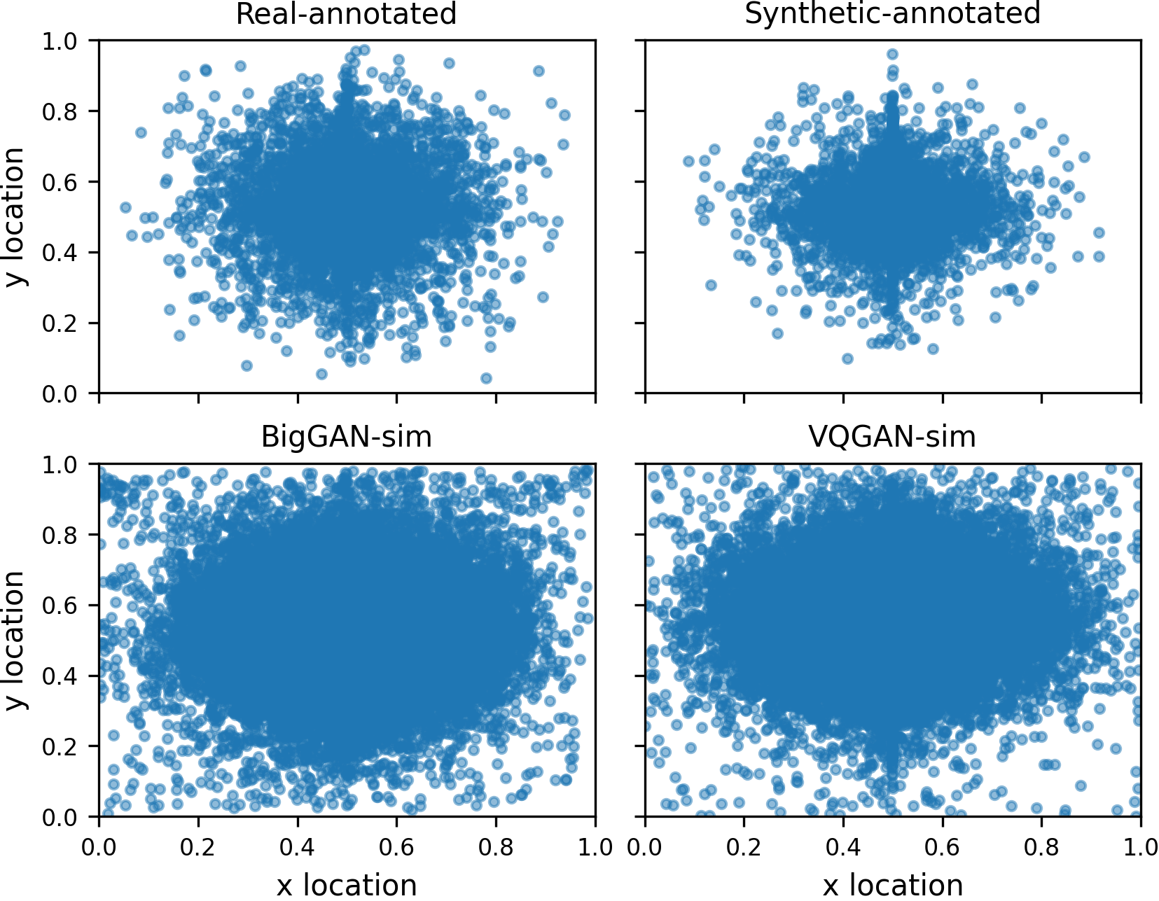
Figure 12: Object center scatter plots. We visualize center positions of the tight bounding box of pixel-wise labels for the Real-annotated, Synthetic-annotated, BigGAN-sim and VQGAN-sim datasets. The box center is normalized with respect to the original image size.

C.1 Center Distributions

We visualize scatter plots of object center locations for the Real-annotated, Synthetic-annotated, BigGAN-sim and VQGAN-sim datasets in Figure 12. We fit a tight bounding box over the segmentation mask and use the center of the bounding box as the center location. Note that the location is normalized with respect to the original image size. We see that most of the object centers are biased towards the image center for all datasets. Compared to the human-annotated datasets, BigGAN-sim and VQGAN-sim show noisier center distributions, in particular towards the image corners.

C.2 Geometry Metrics

In Table 1 in the main paper, we compute geometry metrics to measure shape complexity (SC) and shape diversity (SD) of the human-annotated dataset as well as the synthetic dataset. Here, we provide the corresponding implementation details.

Implementation.

We first filter out masks with a total number of pixels below 100 to avoid noisy labels. We then calculate the connected components in the mask and only use the largest connected component in our measurement. We further use OpenCV’s findContours function with the CHAIN_APPROX_SIMPLE flag which compresses horizontal, vertical, and diagonal segments and leaves only their end points to extract a simplified polygon. Note that the simplification happens in pixel space and the extracted polygons do not have the same scales. In order to overcome such scaling issues, we normalize the extracted polygon to a unit square by $p_{i}=(p_{i}-p_{min})/(p_{max}-p_{min})$ (this operation is applied separately for both horizontal and vertical directions in an image), where $p_{i}$ is the point in the extracted polygon, and $p_{min}$ and $p_{max}$ are the minimum and maximum point coordinates (for either horizontal or vertical direction) over the set of points for a given polygon. We further apply the Douglas-Peucker algorithm [18] with a threshold of $0.01$ to remove redundant points.

Shape Complexity

After applying the pre-processing steps mentioned above, the shape complexity (SC) is calculated as the number of points of the normalized simplified polygon. We also measure polygon length (PL) in Table 1 from the main paper.

Shape Diversity

We calculate the shape diversity by mean pair-wise Chamfer distance [22] per class and average across classes. Specifically, Chamfer distance is defined as

$$d_{\textrm{CD}}(S_{1},S_{2})=\sum_{\mathbf{x}\in S_{1}}\min_{\mathbf{y}\in S_{2}}||\mathbf{x}-\mathbf{y}||^{2}_{2}+\sum_{\mathbf{y}\in S_{s}}\min_{\mathbf{x}\in S_{1}}||\mathbf{x}-\mathbf{y}||^{2}_{2}$$

where $S_{1}$ and $S_{2}$ are sets of points corresponding to different polygons. In our case, we calculate average pair-wise $d_{\textrm{CD}}$ between all polygons within each class. Then, we compute the shape diversity (SD) metric as the average distance over all classes.

Appendix D Transfer Learning Experiments

D.1 Pre-training Implementation

We closely follow the pre-training setup of DenseCL [76], and use SGD as the optimizer with weight decay and momentum set to $0.0001$ and $0.9$, respectively. The dictionary size is set to 65536 and the momentum update rate of the encoder is set to 0.999. We also adopt its augmentation policy with $224\times 224$ random resized cropping, random color jittering, random gray-scale conversion, Gaussian blurring and random horizontal flips for contrastive learning. Note that since texture and color are important hints for semantic segmentation, we only use random resized cropping with resolution 224 $\times$ 224 and random horizontal flip when training the segmentation branch with our synthetic dataset. The batch size is 256, and we train on 8 GPUs with a cosine learning rate decay schedule. We pre-train the backbone on ImageNet using the original contrastive losses for 150 epochs and then jointly train the segmentation branch using the cross-entropy loss for another 50 epochs.

D.2 Downstream Task Details

Benchmark Implementation

For object detection and instance segmentation tasks on Pascal VOC, MS-COCO and Cityscapes, we use standard benchmark configurations from OpenSelfSup. The model is trained using Detectron2 [78]. For semantic segmentation tasks on Pascal VOC and Cityscapes, we use configurations from DenseCL implemented in MMSegmentation [13].

Appendix E Qualitative Results

We show random samples from the human-annotated and synthetic datasets. See Figure 13 for dataset samples from the Real-annotated dataset where annotation is done on real images. Figure 14 shows dataset samples from the Synthetic-annotated dataset where human annotation is on BigGAN generated images. For our synthetic dataset BigGAN-sim generated by BigGAN, see Figure 15, and for the VQGAN-sim dataset generated by VQGAN, see Figure 16. Compared to the synthetic dataset, Real-annotated images have more complex backgrounds and structure. However, we also see that the synthetic datasets generated by BigGAN and VQGAN include photo-realistic and diverse images as well as high quality labels.

We also show per-class samples where images in the same row are from the same class. For BigGAN-sim per-class samples, please see Figure 17. For VQGAN-sim per-class samples, see Figure 18. Note that we select the same classes for both BigGAN-sim and VQGAN-sim for easy comparison. Comparing to BigGAN-sim, the VQGAN-sim dataset samples are more diverse in terms of object scale, pose as well as background. However, we see BigGAN-sim has better label quality than VQGAN-sim where in some cases the labels have holes and are noisy.

We also include mean shape visualizations for different classes from the BigGAN-sim dataset (see Figure 19). We first use a tight bounding box to fit the segmentation, and then crop and resize the segmentation into resolution $32\times 32$. We use k-means clustering with $k=5$ for each class to calculate the major modes of the resized segmentation mask. In Figure 19, we randomly select 500 classes and for each class we randomly select one cluster out of the 5 clusters and visualize the mean shape. We see diverse shapes with different poses especially for classes related to animals. Some classes do not have clear shapes. This might be because the randomly selected mode is potentially not the most meaningful mode.

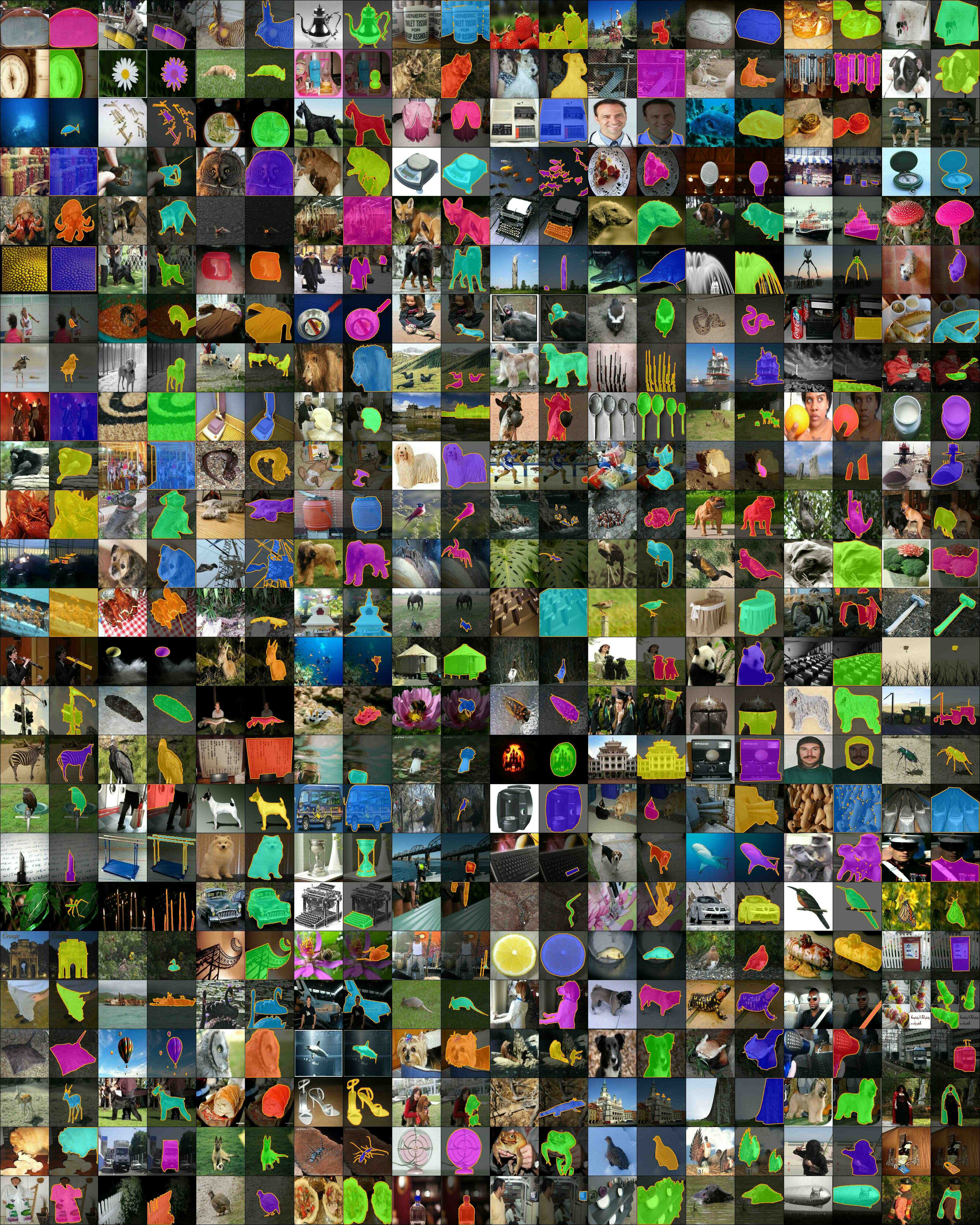
Figure 13: Examples from the Real-annotated dataset. We visualize both the segmentation masks as well as the boundary polygons.

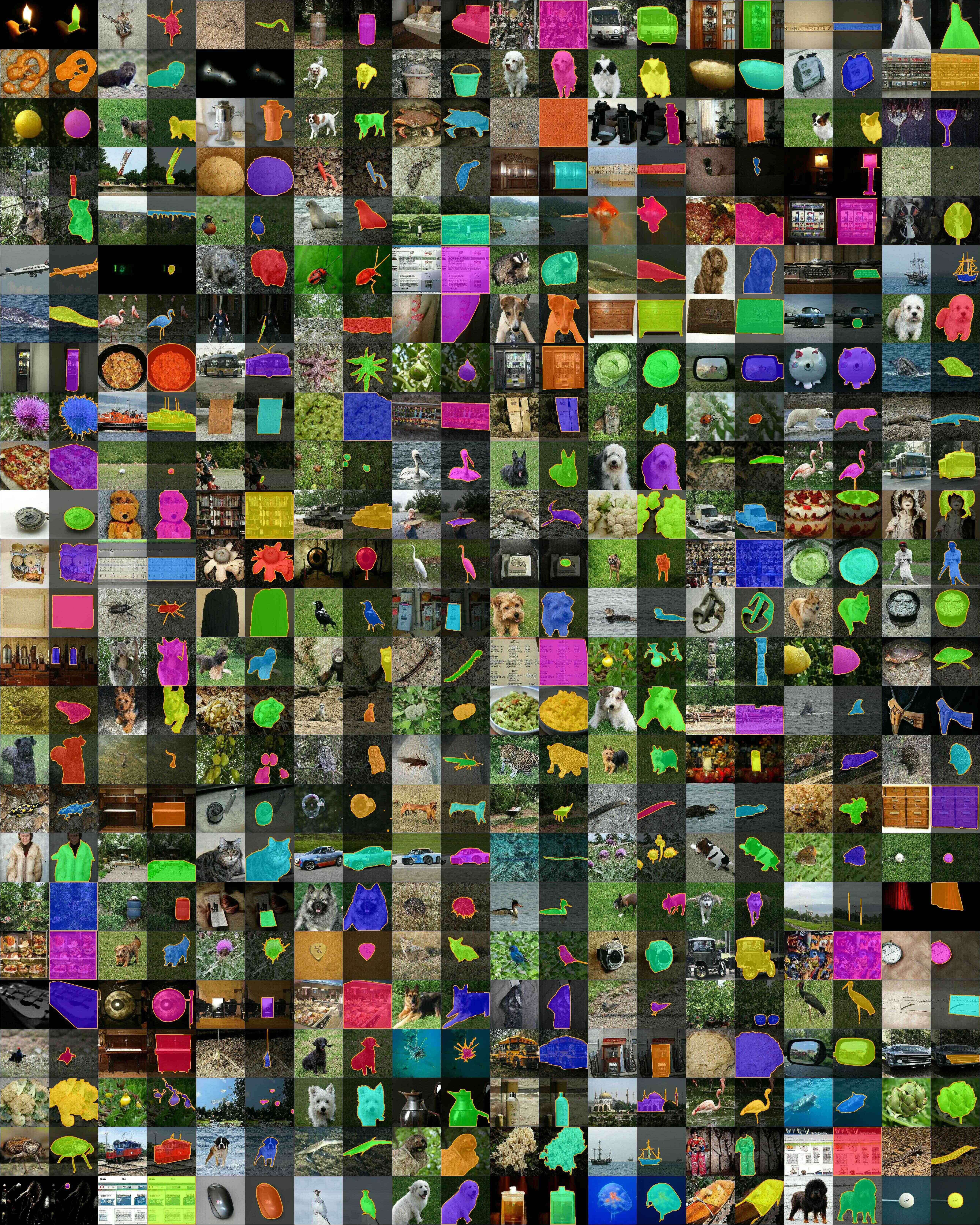
Figure 14: Examples from the Synthetic-annotated dataset. We visualize both the segmentation masks as well as the boundary polygons.

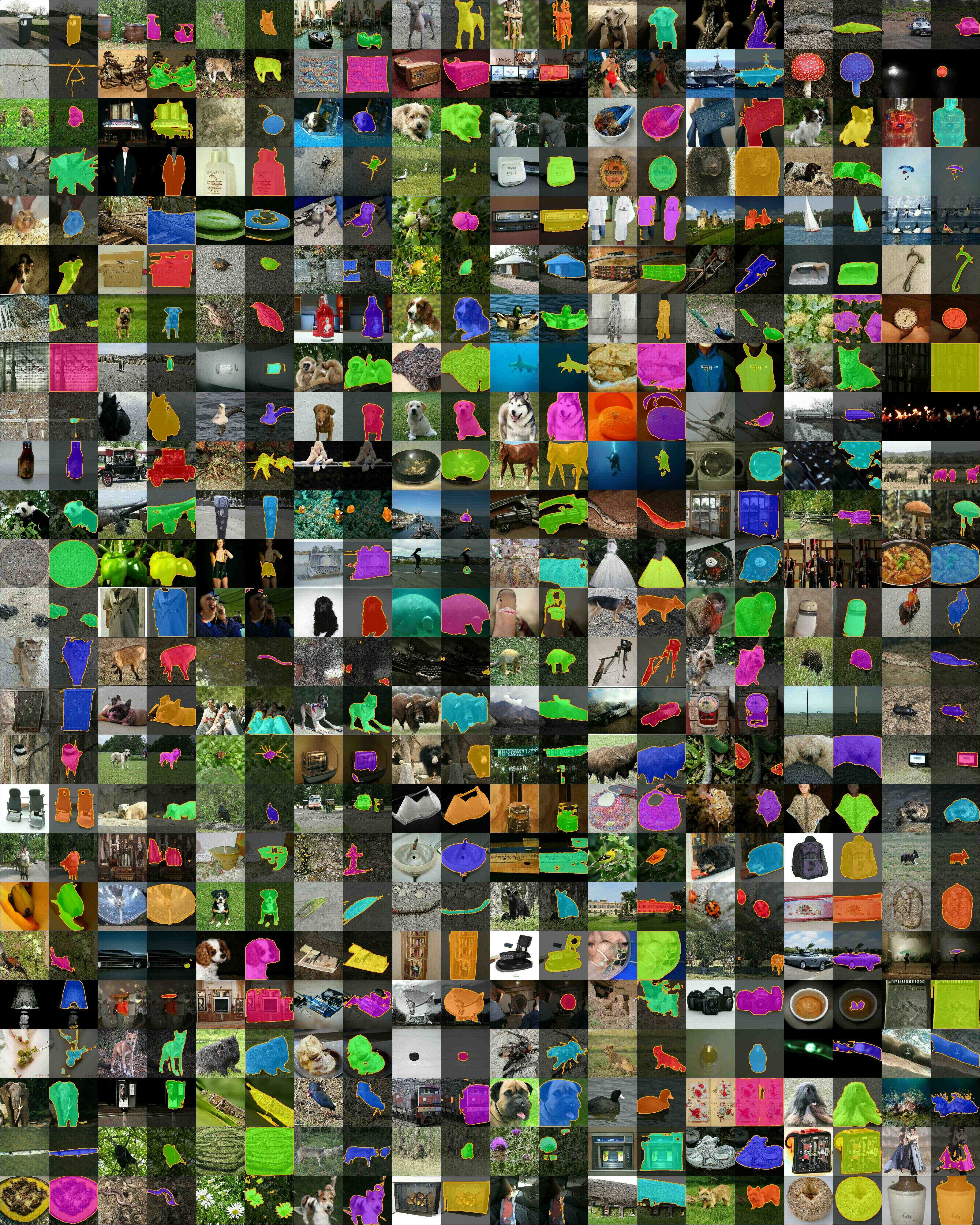
Figure 15: BigGAN-sim random samples. We visualize both the segmentation masks as well as the boundary polygons.

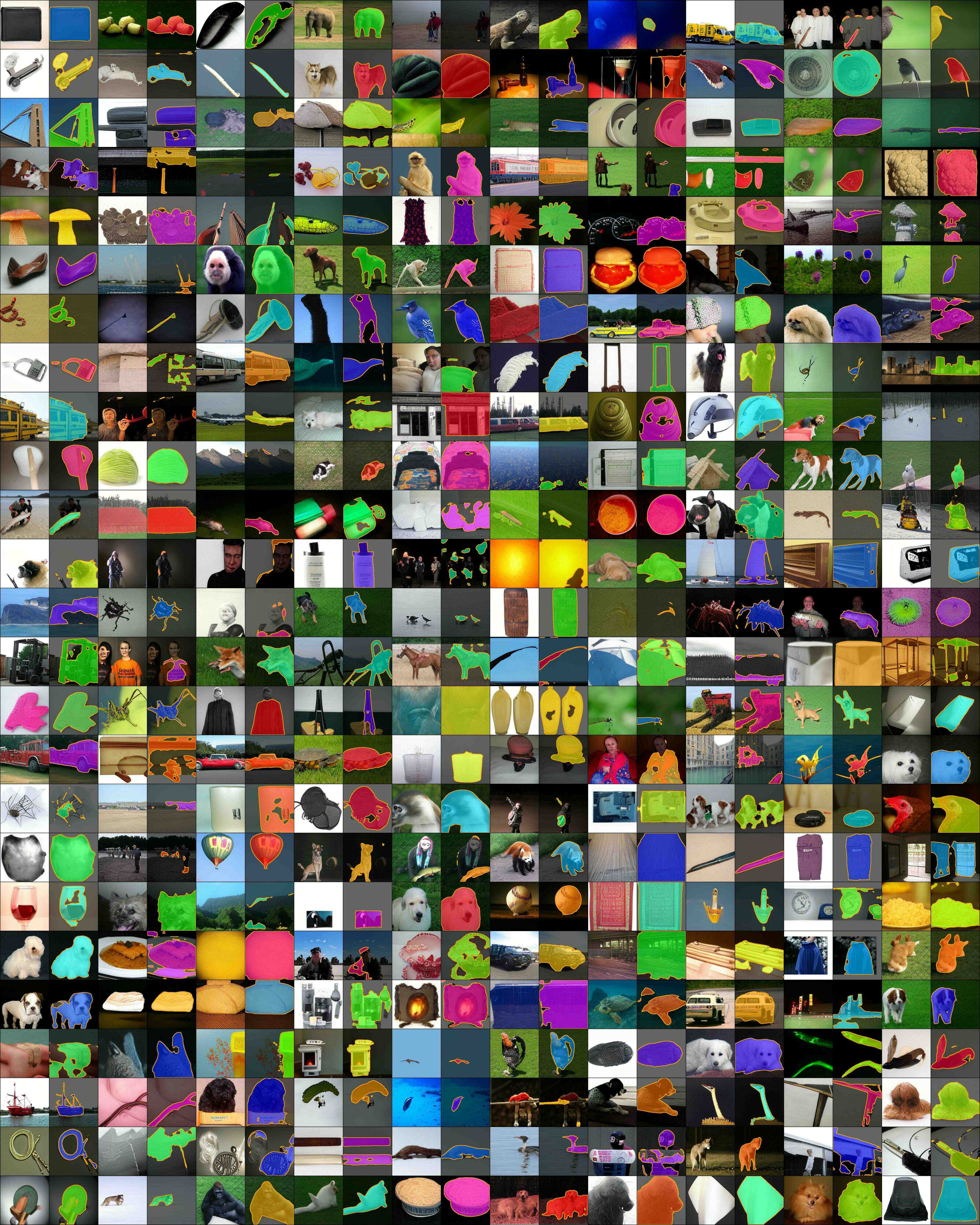
Figure 16: VQGAN-sim random samples. We visualize both the segmentation masks as well as the boundary polygons.

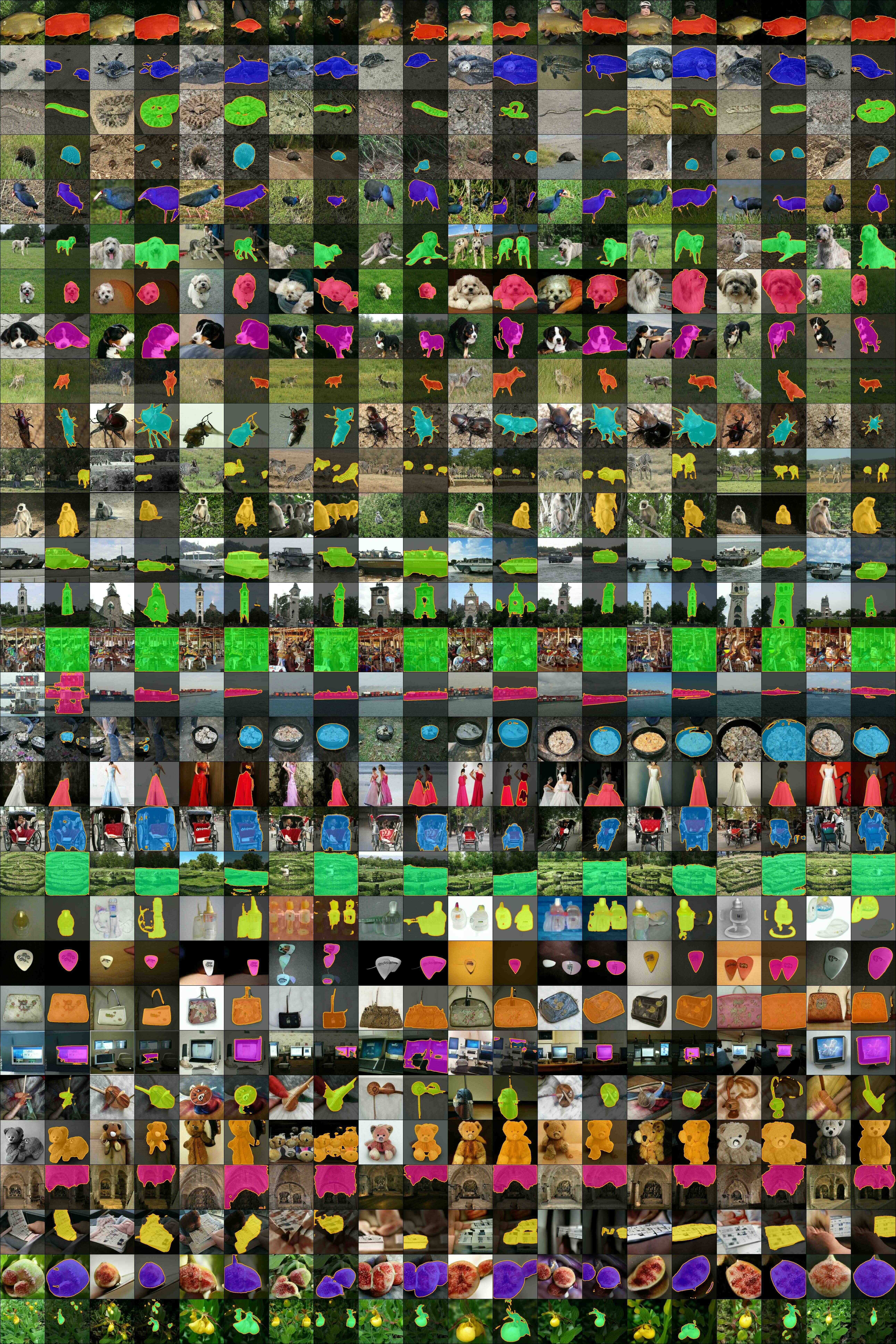
Figure 17: BigGAN-sim per-class samples. We visualize both the segmentation masks as well as the boundary polygons.

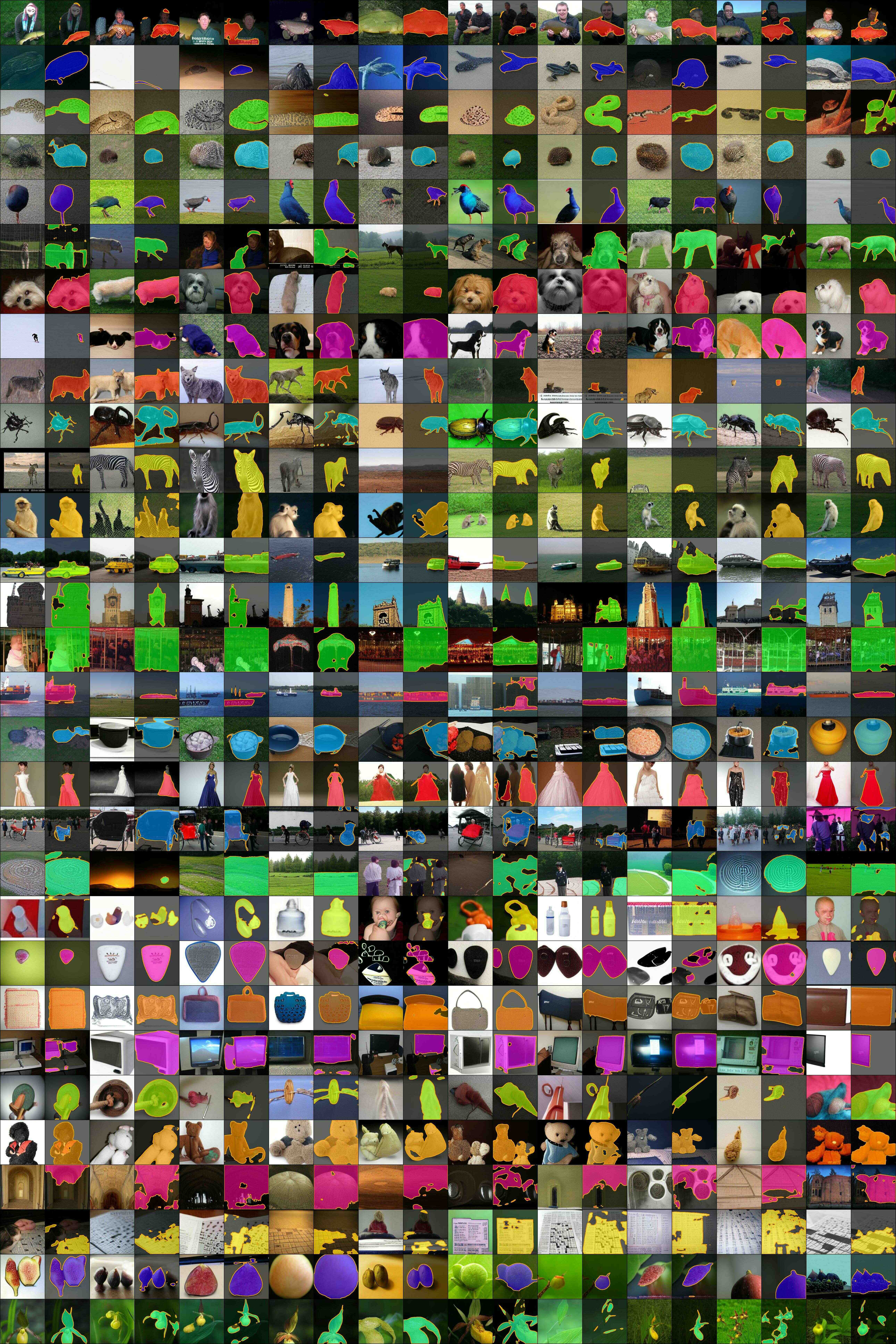
Figure 18: VQGAN-sim per-class samples. We visualize both the segmentation masks as well as the boundary polygons.

Figure 19: BigGAN-sim mean shapes. Mean shapes are calculated using k-means clustering over normalized segmentation masks.

References

- [1] David Acuna, Amlan Kar, and Sanja Fidler. Devil is in the edges: Learning semantic boundaries from noisy annotations. In CVPR, 2019.
- [2] David Acuna, Huan Ling, Amlan Kar, and Sanja Fidler. Efficient annotation of segmentation datasets with polygon-rnn++. In CVPR, 2018.
- [3] Jimmy Lei Ba, Jamie Ryan Kiros, and Geoffrey E Hinton. Layer normalization. arXiv preprint arXiv:1607.06450, 2016.
- [4] William H. Beluch, Tim Genewein, Andreas Nurnberger, and Jan M. Kohler. The power of ensembles for active learning in image classification. In 2018 IEEE/CVF Conference on Computer Vision and Pattern Recognition, pages 9368–9377, 2018.
- [5] Mikołaj Bińkowski, Danica J. Sutherland, Michael Arbel, and Arthur Gretton. Demystifying MMD GANs. In International Conference on Learning Representations, 2018.
- [6] Andrew Brock, Jeff Donahue, and Karen Simonyan. Large scale gan training for high fidelity natural image synthesis, 2019.
- [7] Mathilde Caron, Hugo Touvron, Ishan Misra, Hervé Jégou, Julien Mairal, Piotr Bojanowski, and Armand Joulin. Emerging properties in self-supervised vision transformers, 2021.
- [8] Liang-Chieh Chen, Sanja Fidler, Alan Yuille, and Raquel Urtasun. Beat the mturkers: Automatic image labeling from weak 3d supervision. In CVPR, 2014.
- [9] Liang-Chieh Chen, George Papandreou, Florian Schroff, and Hartwig Adam. Rethinking atrous convolution for semantic image segmentation. arXiv:1706.05587, 2017.
- [10] Ting Chen, Simon Kornblith, Mohammad Norouzi, and Geoffrey Hinton. A simple framework for contrastive learning of visual representations, 2020.
- [11] Xinlei Chen, Haoqi Fan, Ross Girshick, and Kaiming He. Improved baselines with momentum contrastive learning, 2020.
- [12] Xinlei Chen, Saining Xie, and Kaiming He. An empirical study of training self-supervised vision transformers, 2021.
- [13] MMSegmentation Contributors. MMSegmentation: Openmmlab semantic segmentation toolbox and benchmark. https://github.com/open-mmlab/mmsegmentation, 2020.
- [14] Marius Cordts, Mohamed Omran, Sebastian Ramos, Timo Rehfeld, Markus Enzweiler, Rodrigo Benenson, Uwe Franke, Stefan Roth, and Bernt Schiele. The cityscapes dataset for semantic urban scene understanding, 2016.
- [15] Jeevan Devaranjan, Amlan Kar, and Sanja Fidler. Meta-sim2: Unsupervised learning of scene structure for synthetic data generation. In ECCV, 2020.
- [16] Alexey Dosovitskiy, Lucas Beyer, Alexander Kolesnikov, Dirk Weissenborn, Xiaohua Zhai, Thomas Unterthiner, Mostafa Dehghani, Matthias Minderer, Georg Heigold, Sylvain Gelly, Jakob Uszkoreit, and Neil Houlsby. An image is worth 16x16 words: Transformers for image recognition at scale. ICLR, 2021.
- [17] Alexey Dosovitskiy, Germán Ros, Felipe Codevilla, Antonio M. López, and Vladlen Koltun. CARLA: an open urban driving simulator. CoRR, abs/1711.03938, 2017.
- [18] David H Douglas and Thomas K Peucker. Algorithms for the reduction of the number of points required to represent a digitized line or its caricature. Cartographica: the international journal for geographic information and geovisualization, 10(2):112–122, 1973.
- [19] Patrick Esser, Robin Rombach, and Björn Ommer. Taming transformers for high-resolution image synthesis, 2020.
- [20] Mark Everingham, Luc Van Gool, Christopher KI Williams, John Winn, and Andrew Zisserman. The pascal visual object classes (voc) challenge. International journal of computer vision, 88(2):303–338, 2010.
- [21] M. Everingham, L. Van Gool, C. K. I. Williams, J. Winn, and A. Zisserman. The pascal visual object classes (voc) challenge. International Journal of Computer Vision, 88(2):303–338, June 2010.
- [22] Haoqiang Fan, Hao Su, and Leonidas Guibas. A point set generation network for 3d object reconstruction from a single image, 2016.
- [23] Adrien Gaidon, Qiao Wang, Yohann Cabon, and Eleonora Vig. Virtual worlds as proxy for multi-object tracking analysis. In Proceedings of the IEEE conference on computer vision and pattern recognition, pages 4340–4349, 2016.
- [24] Danil Galeev, Konstantin Sofiiuk, Danila Rukhovich, Mikhail Romanov, Olga Barinova, and Anton Konushin. Learning high-resolution domain-specific representations with a gan generator, 2020.
- [25] R. Girshick, J. Donahue, T. Darrell, and J. Malik. Rich feature hierarchies for accurate object detection and semantic segmentation. In CVPR, pages 580–587, 2014.
- [26] Jean-Bastien Grill, Florian Strub, Florent Altché, Corentin Tallec, Pierre H. Richemond, Elena Buchatskaya, Carl Doersch, Bernardo Avila Pires, Zhaohan Daniel Guo, Mohammad Gheshlaghi Azar, Bilal Piot, Koray Kavukcuoglu, Rémi Munos, and Michal Valko. Bootstrap your own latent: A new approach to self-supervised learning, 2020.
- [27] Matthieu Guillaumin, Daniel Küttel, and Vittorio Ferrari. Imagenet auto-annotation with segmentation propagation. International Journal of Computer Vision, 110(3):328–348, 2014.
- [28] Kaiming He, Haoqi Fan, Yuxin Wu, Saining Xie, and Ross Girshick. Momentum contrast for unsupervised visual representation learning, 2020.
- [29] Kaiming He, Georgia Gkioxari, Piotr Dollár, and Ross Girshick. Mask r-cnn. In 2017 IEEE International Conference on Computer Vision (ICCV), pages 2980–2988, 2017.
- [30] Kaiming He, Xiangyu Zhang, Shaoqing Ren, and Jian Sun. Deep residual learning for image recognition. arXiv preprint arXiv:1512.03385, 2015.
- [31] Martin Heusel, Hubert Ramsauer, Thomas Unterthiner, Bernhard Nessler, and Sepp Hochreiter. Gans trained by a two time-scale update rule converge to a local nash equilibrium. In Advances in Neural Information Processing Systems 30, 2017.
- [32] Ari Holtzman, Jan Buys, Li Du, Maxwell Forbes, and Yejin Choi. The curious case of neural text degeneration. arXiv preprint arXiv:1904.09751, 2019.
- [33] Xun Huang, Ming-Yu Liu, Serge J. Belongie, and Jan Kautz. Multimodal unsupervised image-to-image translation. CoRR, abs/1804.04732, 2018.
- [34] Minyoung Huh, Pulkit Agrawal, and Alexei A. Efros. What makes imagenet good for transfer learning?, 2016.
- [35] Ashraful Islam, Chun-Fu Chen, Rameswar Panda, Leonid Karlinsky, Richard Radke, and Rogerio Feris. A broad study on the transferability of visual representations with contrastive learning, 2021.
- [36] Stefan Jaeger, Sema Candemir, Sameer Antani, Yì-Xiáng J Wáng, Pu-Xuan Lu, and George Thoma. Two public chest x-ray datasets for computer-aided screening of pulmonary diseases. Quantitative imaging in medicine and surgery, 4(6):475, 2014.
- [37] Amlan Kar, Aayush Prakash, Ming-Yu Liu, Eric Cameracci, Justin Yuan, Matt Rusiniak, David Acuna, Antonio Torralba, and Sanja Fidler. Meta-sim: Learning to generate synthetic datasets. In ICCV, 2019.
- [38] Tero Karras, Miika Aittala, Samuli Laine, Erik Härkönen, Janne Hellsten, Jaakko Lehtinen, and Timo Aila. Alias-free generative adversarial networks, 2021.
- [39] Tero Karras, Samuli Laine, and Timo Aila. A style-based generator architecture for generative adversarial networks. In Proceedings of the IEEE/CVF Conference on Computer Vision and Pattern Recognition, pages 4401–4410, 2019.
- [40] Tero Karras, Samuli Laine, Miika Aittala, Janne Hellsten, Jaakko Lehtinen, and Timo Aila. Analyzing and improving the image quality of stylegan, 2020.
- [41] Prannay Khosla, Piotr Teterwak, Chen Wang, Aaron Sarna, Yonglong Tian, Phillip Isola, Aaron Maschinot, Ce Liu, and Dilip Krishnan. Supervised contrastive learning, 2021.
- [42] Diederik P. Kingma and Jimmy Ba. Adam: A method for stochastic optimization, 2017.
- [43] Alexander Kirillov, Ross Girshick, Kaiming He, and Piotr Dollár. Panoptic feature pyramid networks, 2019.
- [44] Alex Krizhevsky, Ilya Sutskever, and Geoffrey E. Hinton. Imagenet classification with deep convolutional neural networks. In Advances in Neural Information Processing Systems, pages 1097–1105. 2012.
- [45] Viveka Kulharia, Siddhartha Chandra, Amit Agrawal, Philip Torr, and Ambrish Tyagi. Box2seg: Attention weighted loss and discriminative feature learning for weakly supervised segmentation. In ECCV, 2020.
- [46] Weicheng Kuo, Christian Häne, Esther Yuh, Pratik Mukherjee, and Jitendra Malik. Cost-sensitive active learning for intracranial hemorrhage detection. In MICCAI, 2018.
- [47] Shiyi Lan, Zhiding Yu, Christopher Bongsoo Choy, Subhashree Radhakrishnan, Guilin Liu, Yuke Zhu, Larry Davis, and Anima Anandkumar. Discobox: Weakly supervised instance segmentation and semantic correspondence from box supervision. ArXiv, abs/2105.06464, 2021.
- [48] Daiqing Li, Amlan Kar, Nishant Ravikumar, Alejandro F Frangi, and Sanja Fidler. Federated simulation for medical imaging. In MICCAI, 2020.
- [49] Daiqing Li, Junlin Yang, Karsten Kreis, Antonio Torralba, and Sanja Fidler. Semantic segmentation with generative models: Semi-supervised learning and strong out-of-domain generalization, 2021.
- [50] Di Lin, Jifeng Dai, Jiaya Jia, Kaiming He, and Jian Sun. Scribblesup: Scribble-supervised convolutional networks for semantic segmentation. In CVPR, 2016.
- [51] Tsung-Yi Lin, Priya Goyal, Ross Girshick, Kaiming He, and Piotr Dollár. Focal loss for dense object detection, 2018.
- [52] Tsung-Yi Lin, Michael Maire, Serge Belongie, Lubomir Bourdev, Ross Girshick, James Hays, Pietro Perona, Deva Ramanan, C. Lawrence Zitnick, and Piotr Dollár. Microsoft coco: Common objects in context, 2015.
- [53] Huan Ling, Jun Gao, Amlan Kar, Wenzheng Chen, and Sanja Fidler. Fast interactive object annotation with curve-gcn. In CVPR, 2019.
- [54] Ce Liu, Jenny Yuen, and Antonio Torralba. Nonparametric scene parsing: Label transfer via dense scene alignment. In 2009 IEEE Conference on Computer Vision and Pattern Recognition, pages 1972–1979. IEEE, 2009.
- [55] Jonathan Long, Evan Shelhamer, and Trevor Darrell. Fully convolutional networks for semantic segmentation, 2015.
- [56] K.K. Maninis, S. Caelles, J. Pont-Tuset, and L. Van Gool. Deep extreme cut: From extreme points to object segmentation. In Computer Vision and Pattern Recognition (CVPR), 2018.
- [57] Prem Melville, Stewart M. Yang, Maytal Saar-Tsechansky, and Raymond Mooney. Active learning for probability estimation using jensen-shannon divergence. In João Gama, Rui Camacho, Pavel B. Brazdil, Alípio Mário Jorge, and Luís Torgo, editors, Machine Learning: ECML 2005, pages 268–279, Berlin, Heidelberg, 2005. Springer Berlin Heidelberg.
- [58] Preetum Nakkiran, Behnam Neyshabur, and Hanie Sedghi. The deep bootstrap framework: Good online learners are good offline generalizers, 2021.
- [59] Xingchao Peng, Ben Usman, Neela Kaushik, Judy Hoffman, Dequan Wang, and Kate Saenko. Visda: The visual domain adaptation challenge. arXiv preprint arXiv:1710.06924, 2017.
- [60] Pedro O. Pinheiro, Amjad Almahairi, Ryan Y. Benmalek, Florian Golemo, and Aaron Courville. Unsupervised learning of dense visual representations, 2020.
- [61] Xavier Puig, Kevin Ra, Marko Boben, Jiaman Li, Tingwu Wang, Sanja Fidler, and Antonio Torralba. Virtualhome: Simulating household activities via programs. In CVPR, 2018.
- [62] Ali Razavi, Aaron van den Oord, and Oriol Vinyals. Generating diverse high-fidelity images with vq-vae-2, 2019.
- [63] Shaoqing Ren, Kaiming He, Ross B. Girshick, and Jian Sun. Faster r-cnn: Towards real-time object detection with region proposal networks. In NIPS, pages 91–99, 2015.
- [64] Stephan R Richter, Vibhav Vineet, Stefan Roth, and Vladlen Koltun. Playing for data: Ground truth from computer games. In European conference on computer vision, pages 102–118. Springer, 2016.
- [65] German Ros, Laura Sellart, Joanna Materzynska, David Vazquez, and Antonio M Lopez. The synthia dataset: A large collection of synthetic images for semantic segmentation of urban scenes. In Proceedings of the IEEE conference on computer vision and pattern recognition, pages 3234–3243, 2016.
- [66] A. Rosenfeld and D. Weinshall. Extracting foreground masks towards object recognition. In ICCV, 2021.
- [67] Carsten Rother, Vladimir Kolmogorov, and Andrew Blake. ” grabcut” interactive foreground extraction using iterated graph cuts. ACM transactions on graphics (TOG), 23(3):309–314, 2004.
- [68] Olga Russakovsky, Jia Deng, Hao Su, Jonathan Krause, Sanjeev Satheesh, Sean Ma, Zhiheng Huang, Andrej Karpathy, Aditya Khosla, Michael Bernstein, Alexander C. Berg, and Li Fei-Fei. Imagenet large scale visual recognition challenge, 2015.
- [69] Junji Shiraishi, Shigehiko Katsuragawa, Junpei Ikezoe, Tsuneo Matsumoto, Takeshi Kobayashi, Ken-ichi Komatsu, Mitate Matsui, Hiroshi Fujita, Yoshie Kodera, and Kunio Doi. Development of a digital image database for chest radiographs with and without a lung nodule: receiver operating characteristic analysis of radiologists’ detection of pulmonary nodules. American Journal of Roentgenology, 174(1):71–74, 2000.
- [70] Karen Simonyan and Andrew Zisserman. Very deep convolutional networks for large-scale image recognition. arXiv preprint arXiv:1409.1556, 2014.
- [71] Sergii Stirenko, Yuriy Kochura, Oleg Alienin, Oleksandr Rokovyi, Yuri Gordienko, Peng Gang, and Wei Zeng. Chest x-ray analysis of tuberculosis by deep learning with segmentation and augmentation. In 2018 IEEE 38th International Conference on Electronics and Nanotechnology (ELNANO), pages 422–428. IEEE, 2018.
- [72] Meng Tang, Abdelaziz Djelouah, Federico Perazzi, Yuri Boykov, and Christopher Schroers. Normalized cut loss for weakly-supervised cnn segmentation. In CVPR, 2018.
- [73] J. Tighe and S. Lazebnik. Superparsing: Scalable nonparametric image parsing with superpixels. In ECCV, 2010.
- [74] Nontawat Tritrong, Pitchaporn Rewatbowornwong, and Supasorn Suwajanakorn. Repurposing gans for one-shot semantic part segmentation, 2021.
- [75] Ashish Vaswani, Noam Shazeer, Niki Parmar, Jakob Uszkoreit, Llion Jones, Aidan N Gomez, Łukasz Kaiser, and Illia Polosukhin. Attention is all you need. In Advances in neural information processing systems, pages 5998–6008, 2017.
- [76] Xinlong Wang, Rufeng Zhang, Chunhua Shen, Tao Kong, and Lei Li. Dense contrastive learning for self-supervised visual pre-training, 2021.
- [77] Zian Wang, David Acuna, Huan Ling, Amlan Kar, and Sanja Fidler. Object instance annotation with deep extreme level set evolution. In CVPR, 2019.
- [78] Yuxin Wu, Alexander Kirillov, Francisco Massa, Wan-Yen Lo, and Ross Girshick. Detectron2. https://github.com/facebookresearch/detectron2, 2019.
- [79] Tete Xiao, Colorado J Reed, Xiaolong Wang, Kurt Keutzer, and Trevor Darrell. Region similarity representation learning, 2021.
- [80] Jianjin Xu and Changxi Zheng. Linear semantics in generative adversarial networks. In Proceedings of the IEEE/CVF Conference on Computer Vision and Pattern Recognition, pages 9351–9360, 2021.
- [81] Matthew D. Zeiler and Rob Fergus. Visualizing and understanding convolutional networks. arxiv, 1311.2901, 2013.
- [82] Yuxuan Zhang, Huan Ling, Jun Gao, Kangxue Yin, Jean-Francois Lafleche, Adela Barriuso, Antonio Torralba, and Sanja Fidler. Datasetgan: Efficient labeled data factory with minimal human effort. In CVPR, 2021.