Combined full shape analysis of BOSS galaxies and eBOSS quasars using an iterative emulator

Abstract

Standard full-shape clustering analyses in Fourier space rely on a fixed power spectrum template, defined at the fiducial cosmology used to convert redshifts into distances, and compress the cosmological information into the Alcock-Paczynski parameters and the linear growth rate of structure. In this paper, we propose an analysis method that operates directly in the cosmology parameter space and varies the power spectrum template accordingly at each tested point. Predictions for the power spectrum multipoles from the TNS model are computed at different cosmologies in the framework of $\Lambda\rm{CDM}$. Applied to the final eBOSS QSO and LRG samples together with the low-z DR12 BOSS galaxy sample, our analysis results in a set of constraints on the cosmological parameters $\Omega_{\rm cdm}$, $H_{0}$, $\sigma_{8}$, $\Omega_{\rm b}$ and $n_{s}$. To reduce the number of computed models, we construct an iterative process to sample the likelihood surface, where each iteration consists of a Gaussian process regression. This method is validated with mocks from N-body simulations. From the combined analysis of the (e)BOSS data, we obtain the following constraints: $\sigma_{8}=0.877\pm 0.049$ and $\Omega_{\rm m}=0.304^{+0.016}_{-0.010}$ without any external prior. The eBOSS quasar sample alone shows a $3.1\sigma$ discrepancy compared to the Planck prediction.

1 Introduction

Large scale structures (LSS) bring essential information on how the Universe evolved through the last $10~{}\mathrm{Gyr}$. The current spectroscopic surveys allow the construction of 3D maps of the Universe using biased tracers of matter (e.g. galaxies or quasars). In standard clustering analyses, the information encoded in the power spectrum of the tracer distribution in redshift space is compressed into three parameters: the Alcock-Paczynski parameters ($\alpha_{\parallel}$ and $\alpha_{\perp}$) that constrain the cosmological distances through the position of the baryon acoustic oscillations features (BAO) and the amplitude of velocity fluctuations $f\sigma_{8}$ measured from the clustering power as a function of the angle with respect to the line-of-sight.

This compression is accurate but not exact as the information from the shape of the power spectrum is ignored (Brieden et al., 2021). In standard analyses, a fiducial cosmology is chosen to compute both the distances from object redshifts and the model power spectrum. In this case, the cosmological constraints extracted from the data present a dependency in the fiducial cosmology that requires to be treated as a systematic error (Smith et al., 2020).

Recently, the eBOSS collaboration performed BAO and full shape (BAO+RSD) analyses at different epochs of the Universe evolution, from $z=0.6$ to $z=2.2$, in Fourier and configuration spaces (Gil-Marín et al., 2020; Bautista et al., 2021; de Mattia et al., 2021; Tamone et al., 2020; Neveux et al., 2020; Hou et al., 2021). The information from each tracer was compressed into a radial distance, a transverse distance and the growth rate of structures at each effective redshift. The eBOSS cosmological analysis (eBOSS Collaboration et al., 2020) was performed by fitting cosmological parameters onto these compressed quantities and showed that the inferred bias from the dependency in the fiducial cosmology was low enough regarding eBOSS statistical power but has to be considered for next-generation surveys like DESI (Collaboration et al., 2016) or Euclid (Amendola et al., 2018). Besides, different techniques have been used to take into account the full shape of the power spectrum, avoiding the compression step to directly constraint base cosmological parameters and accounting for the full shape of the power spectrum (Sánchez et al., 2017; Grieb et al., 2017; Tröster et al., 2020; Semenaite et al., 2021), and more recently, using the Effective Field Theory approach (Ivanov et al., 2020; d’ Amico et al., 2020; Colas et al., 2020; Chen et al., 2021; Zhang & Cai, 2021).

In the present analysis, we use a given cosmology to convert redshifts into distances to compute the data power spectrum. On the other hand, we evaluate the model power spectrum for different cosmologies in the $\Lambda$CDM framework and compare the measured power spectrum to each model, letting nuisance parameters free while the informative parameters ($\alpha_{\parallel}$, $\alpha_{\perp}$ and $f\sigma_{8}$) take their values as predicted in each considered cosmology. In this way, we are able to reconstruct the likelihood surface directly in the cosmological parameter space. We use the TNS model (Taruya et al., 2010) where calculation are done in the RegPT framework with correction computed at two loops (Taruya et al., 2012). Computing the model takes around 300 cpu hour per point, which is too expensive to be used in a Monte Carlo Markov Chain algorithm. To circumvent this problem, we construct an iterative emulator based on the algorithm presented in Pellejero-Ibañez et al. (2020). Emulation has been gaining a lot of interest, as it allows to speed up the analysis by reducing the number of expensive function evaluations required by allowing to interpolate between model predictions at a set of points in the parameter space. This method has been used in a number of galaxy clustering analyses to directly emulate observables such as galaxy power spectrum (Kwan et al., 2015) and correlation function (Zhai et al., 2019) or model ingredients such as the redshift space power spectrum of halos (Kobayashi et al., 2021). Nevertheless, when building an emulator one must consider how theory model uncertainty might propagate to the cosmological parameter space which is non-trivial and needs to be validated for each new statistic or range of scales employed. The algorithm presented by Pellejero-Ibañez et al. (2020) aims at dealing this challenge by emulating the likelihood function directly, which additionally simplifies the process of building the emulator by reducing the dimensions of the emulated quantity. It allows us to compute 100-1000 fewer models to span the cosmological parameter space and interpolate the whole likelihood surface by running a Gaussian process regression at each iteration.

In section 2, we present the surveys we analysed as well as the mocks used to test our pipeline, section 3 presents the method, and section 4 lists the results obtained on mocks and on the (e)BOSS data.

2 Catalogues and mocks

In this section, we present the BOSS and eBOSS data sets used in this work and describe the mocks built from the OuterRim N-body simulations used to test the analysis.

2.1 Data power spectrum

We analyse hereafter three samples of the SDSS collaboration (Blanton et al., 2017); the QSO and LRG sample of the extended Baryon Oscillation Spectroscopic Survey (eBOSS; Dawson et al. (2016)) and the low-z galaxy sample of BOSS (Dawson et al., 2013). Those data have been taken using the optical spectrograph of BOSS (Smee et al., 2013) in the 2.5m Sloan Foundation Telescope (Gunn et al., 2006). The quasars and galaxies target selections are presented in Myers et al. (2015) and Prakash et al. (2016), respectively. We summarise, here, the statistic of those samples:

• the eBOSS DR16 low-z quasar sample ($0.8<z<2.2$) including $343\,708$ objects,

• the eBOSS DR16 LRG sample ($0.6<z<1.0$) including $377\,458$ objects,

• the BOSS DR12 low-z LRG sample ($0.2<z<0.5$) including $604\,002$ objects.

Our study is performed in Fourier space, and for the data part, we profit from all the results provided by the SDSS collaboration (Beutler et al., 2017; Gil-Marín et al., 2020; Neveux et al., 2020). This includes power spectrum multipole measurements, window functions and fast mock power spectra used to compute the covariance matrix. The three samples are divided into northern (NGC) and southern (SGC) galactic caps. The k-ranges used in this work are the same as those used in each of the standard analyses and are summarised in table 1. Notice that the window functions are normalised following the normalisation of the power spectrum to ensure the consistency of the analysis (de Mattia & Ruhlmann-Kleider, 2019).

Table 1: $k$-range used for the 3 (e)BOSS surveys.

Survey	Multipole	$k$-range $\rm~{}[h\cdot Mpc^{-1}]$
QSO DR16	$[0,2,4]$	$[0.02,0.30]$
LRG DR16	$[0,2,4]$	$[0.02,0.15]$
low-z galaxies DR12	$[0,2]$	$[0.02,0.15]$
	$[4]$	$[0.02,0.1]$

The eBOSS LRG and quasar samples slightly overlap at redshift $0.8<z<1.0$. However, it consists of a relatively small part of the LRG sample. Following eBOSS analysis, the correlation has been estimated to be less than 0.1 and is neglected. For BOSS DR12, we use only the low-z part of the sample since the highest redshift part is included in the eBOSS DR16 sample. For the sake of simplifying the analysis, the BOSS galaxies within $0.5<z<0.6$ are ignored.

We use the fast mock power spectra provided with each sample to compute the covariance matrices for the individual likelihood computations, consistently with the individual analyses. Those power spectra are computed assuming the same redshift to distance relation as the data power spectrum.

2.2 QSO mocks

To test the analysis, we make use of mocks constructed from the OuterRim N-body simulation (Habib et al., 2016). This simulation contains $10\,240^{3}$ dark matter particles of mass $m=1.85.10^{9}~{}\mathrm{M_{\sun}h^{-1}}$ in a box of length $L=3h^{-1}Gpc$ with periodic boundary conditions. It was produced with a flat $\Lambda\mathrm{CDM}$ cosmology:

$$\begin{split}h=0.71,\,\,\Omega_{\rm cdm}\mathrm{h}^{2}=0.1109,\,\,\Omega_{\rm b}\mathrm{h}^{2}=0.02258,\\ \sigma_{8}=0.8,\,\,\mathrm{n_{s}}=0.963.\qquad\end{split}$$ (1)

We use QSO mocks built from one snapshot at $z=1.433$ of the OuterRim simulation as explained in Smith et al. (2020). We use a halo occupation distribution (HOD) that is a function of the halo mass, composed by a top hat function to populate halos with central quasars and a power law for satellites. This HOD is used as our baseline in the following and is described in more details in Smith et al. (2020) where it is called "mock2". It was chosen as it is very well fit by the TNS model described in Sec 3.3. Therefore, we ensure that a difference in the cosmological inference of the present analysis would be due to our technique and not to the response of the TNS model to this particular HOD. We average the power spectra over 100 realisations for this particular HOD.

The covariance matrix is rescaled considering that these 100 realisations are independent. As all realisations come from a unique dark matter distribution and so are not strictly independent, errors may be underestimated.

From the same snapshot, we also use alternative mocks built with a different HOD, called "mock4" in Smith et al. (2020). This HOD combines a smooth step function for central quasars and a power law for satellites that corresponds to a more physical HOD for quasars.

3 Analysis method

We present here the general pipeline based on Pellejero-Ibañez et al. (2020) and explain the different steps in more detail in the following subsections.

1. We compute the data power spectrum for a given fiducial cosmology.

2. We create a Latin Hypercube sampling (LHS) to span the cosmological parameter space efficiently.

3. We compute all cosmology-dependent terms of the model power spectrum for each point of the LHS and each effective redshift of the data using the 2-loop correction TNS model.

4. For each point of the LHS, we fit the full model power spectrum to the data, minimizing only over nuisance parameters (as informative parameters are set to their true value in each model). Therefore, we obtain a likelihood value at each point.

5. We use a Gaussian process to interpolate the likelihood surface in the cosmological parameter space.

6. We select new points in the cosmological parameter space using the acquisition function to compute new power spectrum models.

7. We fit those new model power spectra to the data, minimizing over nuisance parameters, and again run a Gaussian process.

8. The two last points are iterated up to the convergence of the estimate likelihood distribution.

3.1 Data power spectrum

We use the data power spectra provided by the SDSS collaboration which have been all computed within the fiducial cosmology:

$$\begin{split}h=0.676,\,\,\Omega_{m}=0.31,\,\,\Omega_{b}h^{2}=0.022,\\ \sigma_{8}=0.8,\,\,n_{s}=0.97\qquad\end{split}$$ (2)

3.2 Latin Hypercube Sampling

To span the cosmological parameter space efficiently, we use a 5D Latin Hypercube sampling (LHS). Assuming $n$ is the number of cosmological parameters, the LHS technique consists of dividing each dimension of the parameter space into $n$ intervals. Then, for each parameter, the $n$ intervals are filled only once, thereby enforcing minimal distance between points compared to a random Poisson sampling.

The cosmological parameter space chosen for this work encompasses large variations in order to avoid biasing the analysis:

$$\begin{split}\Omega_{\rm cdm}=[0.05,0.9],\sigma_{8}=[0.65,1.5],\Omega_{\rm b}=[0.015,0.066],\\ n_{s}=[0.8,1.15],H_{0}=[61,76].\end{split}$$ (3)

Those ranges can be seen as a set of wide flat priors.

3.3 Model power spectrum

To model the power spectrum, we use the RegPT treatment of the TNS model (Taruya et al., 2012). In this framework, the redshift space tracer power spectrum is given by

$$P_{\mathrm{t}}(k,\mu) =D(k,\mu,\sigma_{v},a_{\rm vir})\left[P_{\mathrm{t},\delta\delta}(k)+2f\mu^{2}P_{\mathrm{t},\delta\theta}(k)\right.$$

$$\left.+f^{2}\mu^{4}P_{\theta\theta}(k)+b_{1}^{3}A(k,\mu,f/b_{1})+b_{1}^{4}B(k,\mu,f/b_{1})\right],$$ (4)

where the wavenumber $k$ is the norm of the wavevector $\mathbf{k}$ and $\mu$ its cosine angle with respect to the line-of-sight. $f$ is the linear growth rate of structure.

Here, $P_{\mathrm{t},\delta\delta}(k)$ and $P_{\mathrm{t},\delta\theta}(k)$ are the tracer-tracer and tracer-velocity power spectra, respectively, and are given by:

$$P_{\mathrm{t},\delta\delta}(k) =b_{1}^{2}P_{\delta\delta}(k)+2b_{2}b_{1}P_{b2,\delta}(k)+2b_{s2}b_{1}P_{bs2,\delta}(k)$$

$$+2b_{3\mathrm{nl}}b_{1}\sigma_{3}^{2}(k)P_{\mathrm{m}}^{\mathrm{lin}}(k)+b_{2}^{2}P_{b22}(k)$$

$$+2b_{2}b_{s2}P_{b2s2}(k)+b_{s2}^{2}P_{bs22}(k)+N_{g},$$ (5)

and:

$$P_{\mathrm{t},\delta\theta}(k) =b_{1}P_{\delta\theta}(k)+b_{2}P_{b2,\theta}(k)$$

$$+b_{s2}P_{bs2,\theta}(k)+b_{3\mathrm{nl}}\sigma_{3}^{2}(k)P_{\mathrm{m}}^{\mathrm{lin}}(k),$$ (6)

where $b_{1}$ is the linear bias, $b_{2}$ the second order local bias, $b_{s2}$ the second order non-local bias, $b_{3nl}$ the third order non local bias and $N_{g}$ the constant stochastic term. Assuming local Lagrangian bias, and following Saito et al. (2014), we set the non-local biases to:

$$b_{s2} =-\frac{4}{7}\left(b_{1}-1\right),$$ (7)

$$b_{3\mathrm{nl}} =\frac{32}{315}\left(b_{1}-1\right).$$ (8)

We also assume no velocity bias, $P_{t,\theta\theta}=P_{\theta\theta}$.

In this work, at each point in the cosmological parameter space we compute the linear matter power spectrum with CLASS and evaluate the non-linear matter power spectra $P_{\delta\delta}$,$P_{\delta\theta}$ and $P_{\theta\theta}$, as well as RSD correction terms $A(k,\mu,f/b_{1})$ and $B(k,\mu,f/b_{1})$ at the 2-loop order, these last terms taking most of the computing time. The $1$-loop bias terms $P_{b2,\delta}(k)$, $P_{bs2,\delta}(k)$, $\sigma_{3}^{2}(k)$, $P_{b2,\theta}(k)$ and $P_{bs2,\theta}(k)$ are provided in Beutler et al. (2017).

Finally, to account for non-linear effects, we include an overall damping function,

$$D(k,\mu,\sigma_{v},a_{\rm vir})=\frac{1}{\sqrt{1+(k\mu a_{\rm vir})^{2}}}\exp{\left[-\frac{(k\mu\sigma_{v})^{2}}{1+(k\mu a_{\rm vir})^{2}}\right]}.$$ (9)

As explained in Neveux et al. (2020), this prescription allows to dissociate the Gaussian and the non-Gaussian part of the small scale non-linear effects, through the parameters $\sigma_{v}$ and $a_{\rm vir}$, respectively. This damping term stands for the Finger-of-God effect as well as the redshift uncertainty. This damping term is based on the Finger-of-God of Sánchez et al. (2017), where we removed the $f$-dependency. Such an empirical term has been shown to correctly model various redshift smearing schemes in the eBOSS mock quasar challenge (Smith et al., 2020). Altogether, the model power spectrum is thus described by 5 nuisance parameters ($b_{1}$, $b_{2}$, $N_{g}$, $\sigma_{v}$ and $a_{\rm vir}$).

We make use of the model implementation of de Mattia et al. (2021), which has been tested against mocks as part of the eBOSS mock challenge (Alam et al., 2020; Smith et al., 2020) for redshifts $z=0.859$ and $z=1.433$. Those tests state that the main systematic error arises when using a template model cosmology different from the truth. Considering the tests when cosmologies match, the mock challenge indicates errors smaller than 3% for $f\sigma_{8}$ and 0.5% for the $\alpha$ at both redshifts. Note that the model power spectrum requires to include the survey window function which is computed with the same fiducial cosmology as that used to estimate the data power spectrum.

3.4 Scaling the power spectrum

In standard clustering analyses, the same cosmology is used for the fiducial cosmology and the power spectrum model, and the scale factors are left free in the fitting procedure to recover the underlying cosmology. In this work, each template power spectrum model is evaluated in a cosmology that is different from the fiducial cosmology used to convert redshifts into distances. This difference produces geometrical distortions evaluated through the Alcock-Paczynski (AP) test (Alcock & Paczynski, 1979) that are exactly accounted for by introducing two scaling factors:

$$\alpha_{\parallel}=\frac{D_{\rm H}^{\rm true}(z)}{D_{\rm M}^{\rm fid}(z)},\qquad\alpha_{\perp}=\frac{D_{\rm M}^{\rm true}(z)}{D_{\rm M}^{\rm fid}(z)},$$ (10)

for the line-of-sight and the transverse components, respectively, with distances evaluated in $\rm Mpc$. Then, the wavenumber observed with the fiducial cosmology $k$ and the true wavenumber $k^{\prime}$ are related by $k_{\|}^{\prime}=k_{\|}/\alpha_{\|}$ and $k_{\perp}^{\prime}=k_{\perp}/\alpha_{\perp}$. Transferring this into $k=\sqrt{k_{\|}^{2}+k_{\perp}^{2}}$ and $\mu$ the cosine with the line-of-sight leads to:

$$\begin{split}k&{}^{\prime}=\frac{k}{\alpha_{\perp}}\left[1+\mu^{2}\left(\left(\frac{\alpha_{\perp}}{\alpha_{\|}}\right)^{2}-1\right)\right]^{1/2}\\ \mu^{\prime}&=\mu{\frac{\alpha_{\perp}}{\alpha_{\|}}}\left[1+\mu^{2}\left(\left(\frac{\alpha_{\perp}}{\alpha_{\|}}\right)^{2}-1\right)\right]^{-1/2}.\\ \end{split}$$ (11)

The above $(k,\mu)\rightarrow(k^{\prime},\mu^{\prime})$ mapping must be used together with Equation 4 to include the AP effect in the model power spectrum to be compared to data (see Equation 19 of de Mattia et al. (2021)).

In this work, we operate directly in the $\Lambda\mathrm{CDM}$ framework and the likelihood surface we build is expressed as a function of 5 cosmological parameters, $\Omega_{\rm cdm},\sigma_{8},n_{s},\Omega_{\rm b}$ and $H_{0}$, where $\sigma_{8}$ is the normalisation of the linear power spectrum at redshift $z=0$. Values of the standard parameters $\alpha_{\perp,\parallel}$ and $f\sigma_{8}(z)$ at any redshift of interest can be inferred from those of the cosmological parameters, using equation 10 for the dilation scales and taken from CLASS for the linear growth rate of structure $f$.

3.5 Fit of nuisance parameters

For each model under test and for each galactic cap of each tracer, we find the best-fit nuisance parameters by maximizing the likelihood function,

$$L\propto e^{-\chi^{2}/2},$$ (12)

with

$$\chi^{2}=(P_{\rm data}-P_{\rm model}(\theta))^{t}W(\rm P_{data}-P_{\rm model}(\theta)),$$ (13)

where $P_{\rm data}$ is the data vector of power spectrum multipoles and $P_{\rm model}$ is the corresponding vector for the model that is a function of the parameters. We perform the $\chi^{2}$ minimisation using the code MINUIT. The inverse of the covariance matrix, $W$, is computed from mocks and corrected for the finite number of mocks following the Hartlap et al. (2007) prescription:

$$W=\frac{N-n-2}{N-1}C^{-1},$$ (14)

with $N$ the number of mocks used in the construction of the covariance matrix and $n$ the size of the data vector. Following Percival et al. (2014) and in line with standard analyses, we apply an additional scaling on the cosmological parameter covariance that results in an increase of the errors of the order of a few per cent.

Then, for each point of the parameter space under consideration, the final data likelihood is obtained by taking the product of likelihoods for each tracer (QSO, LRG) and galactic caps (NGC, SGC), maximising its value over the five free nuisance parameters of the model (see section 3.3) for each tracer.

3.6 Gaussian process

To interpolate the likelihood surface in the 5-dimensional cosmological parameter space, we use a non-parametric technique that gives us the expected likelihood value at every point of the parameter space and the error on this interpolation. Two hypotheses must be verified to perform an efficient Gaussian process. The interpolated points have to be within the convex hull formed by the computed points. We use the approximation of restricting the interpolation interval by 5% for all parameters. The second hypothesis is that the surface to interpolate must be smooth enough; a small deviation in the hyper-parameter space must induce a small deviation in the function. We expect the log-likelihood surface to follow this statement.

We use a Gaussian process to estimate the value of the logarithm of the likelihood at a point (in the cosmological parameter space) $\boldsymbol{y}$, $f_{y}={\rm log}L(\boldsymbol{y})$, knowing the value of the likelihood on a set of points $X~{}=~{}\{\boldsymbol{x}_{1},\boldsymbol{x}_{2},...,\boldsymbol{x}_{N}\}$, $\boldsymbol{f}_{X}={\rm log}L(X)$. We must evaluate the probability distribution of $f_{y}$ knowing $\boldsymbol{f}_{X}$; $p(f_{y}|\boldsymbol{f}_{X},X,y)$. Assuming that the joint distribution of $\boldsymbol{f}_{X}$ and $f_{y}$ is Gaussian,

$$p(\boldsymbol{f}_{X},f_{y})=\mathcal{N}\begin{pmatrix}\begin{pmatrix}\boldsymbol{\mu}_{x}\\ \mu_{y}\end{pmatrix},\begin{pmatrix}K_{X}&K_{Xy}\\ K_{Xy}^{T}&K_{y}.\end{pmatrix}\end{pmatrix}$$ (15)

As in a standard Gaussian emulator analysis, we assume the central values of the multivariate Gaussian distribution to be $\mu_{x}=\mu_{y}=0$. The interpolation is entirely governed by the covariance terms, $K_{X}$ referring to the covariance of $\boldsymbol{f}_{X}$, $K_{y}$ the (scalar) covariance of $f_{y}$, and $K_{Xy}$ the (vector) covariance between $\boldsymbol{f}_{X}$ and $f_{y}$.

From $p(\boldsymbol{f}_{X},f_{y})$ and using the multivariate normal theorem we may calculate the conditional probability distribution as

$$p(f_{y}|\boldsymbol{f}_{x})=\mathcal{N}\left(\boldsymbol{\mu}_{\rm interp},K_{\rm interp}\right)$$ (16)

with

$$\boldsymbol{\mu}_{\rm interp}=K_{Xy}K_{y}^{-1}\boldsymbol{f}_{X}$$ (17)

$$K_{\rm interp}=K_{X}-K_{Xy}K_{y}^{-1}K_{Xy}^{T}$$ (18)

In these expressions, $\boldsymbol{f}_{X}$ is known and we need to choose a form for the covariances. For this analysis where we expect the interpolated surface to vary smoothly, we choose the covariance (also called kernel) $K$ to be a linear combination of a squared exponential (or radial basis function) and a linear kernel:

$$K_{i,j}=\sigma_{\rm rbf}e^{-\frac{(\boldsymbol{x}_{i}-\boldsymbol{x}_{j})^{2}}{l_{\rm rbf}}}+\delta_{D}(i-j)\sigma_{\rm fit},$$ (19)

where $K_{i,j}$ is the covariance between point $\boldsymbol{x}_{i}$ and $\boldsymbol{x}_{j}$, $\sigma_{\rm rbf}$ represents the amplitude of the variance, $l_{\rm rbf}$ the characteristic interpolation length-scale and $\sigma_{\rm fit}$, the possible error in the determination of $\boldsymbol{f}_{X}$.

In the Gaussian Process package that we use (GPy, 2012), these three hyper-parameters are common to the five cosmological parameters, therefore we scale parameters by the standard deviation of current points X. The hyper-parameters are let free and fitted by maximizing the marginal log-likelihood of the probability function of the known points (Rasmussen & Williams, 2005):

$$\log p(\boldsymbol{f}_{X}|X,K)=-\frac{1}{2}\boldsymbol{f}_{X}^{T}K^{-1}\boldsymbol{f}_{X}-\frac{1}{2}\log|K|-\frac{N}{2}\log(2\pi),$$ (20)

with $N$, the number of points of the training sample.

In a five-dimensional parameter space, even an algorithm as fast as the Gaussian process interpolation would take too long to run on a dense grid spanning the parameter space, therefore we run a Markov Chain Monte Carlo (MCMC) to obtain the interpolated log-likelihood hypersurface at each iteration step.

One may further include additional priors when performing such sampling of the Gaussian process interpolation. In this analysis (see section 4.2), we study the impact of Gaussian priors: a prior on $\omega_{b}=0.0222\pm 0.0005$ inspired by the Big Bang Nucleosynthesis (BBN) analysis, and a prior on $n_{s}=0.96\pm 0.02$, which are the minimal priors used in eBOSS Collaboration et al. (2020).

3.7 New iteration and convergence

To check that the Gaussian process prediction has converged, we calculate new model power spectra. The choice of new points is done using an acquisition function $A(\boldsymbol{x})$ that, in the general case, accounts for the interpolated log-likelihood and the error on the interpolation, $\sigma$:

$$A(\boldsymbol{x})=\log L_{\rm interp}(\boldsymbol{x})+\alpha\sigma_{\log L_{\rm interp}}(\boldsymbol{x}))$$ (21)

where $\alpha$ is a free parameter that we set to 0 in our standard analysis. This gives an acquisition function that just accounts for the value of the interpolated likelihood to maximize the time spent to refine the region of space with high likelihood. Tests performed with a non-zero value of $\alpha$ did not show any improvement.

The likelihood is computed at 10 points sampled from $A(\boldsymbol{x})$, which we add to previously computed points for a new Gaussian process regression; such procedure is repeated until convergence. This is tested by computing the Kullback-Leibler divergence between the estimated likelihood distributions at iterations $i$ and $i-1$, namely:

$$\begin{split}&D_{\rm KL}(\log L_{\rm interp,i}||\log L_{\rm interp,i-1})=\\ &\frac{1}{2}\left[\log\frac{|C_{i-1}|}{|C_{i}|}-d+tr(C_{i-1}^{-1}C_{i})+(\mu_{i-1}-\mu_{i})^{T}C_{i-1}^{-1}(\mu_{i-1}-\mu_{i})\right]\end{split}$$ (22)

where $d$ is the dimension of the parameter space. Consistently with Pellejero-Ibañez et al. (2020), we require the condition $D_{\rm KL}<0.1$ to be fulfilled to stop the iterative procedure.

4 Results

In this section, we first study the efficiency of our analysis on mocks. The accuracy of the TNS model as well as the impact of observational systematics were evaluated in Beutler et al. (2017); Gil-Marín et al. (2020); Neveux et al. (2020) and are not repeated here. Then, we present the results on BOSS and eBOSS data.

4.1 Results on QSO mocks

Our pipeline was tested on the mocks of section 2.2 to evaluate the performance of our full 5-D cosmological parameter space analysis.

4.1.1 Impact of the fiducial cosmology

Although the power spectrum template is varied throughout the cosmological parameter space, we check the dependence of the cosmological constraints with the fiducial cosmology chosen to convert redshifts to distances. Different tests were run to study this dependence, with results summarized in Table 2 and figure 1. We first take the OuterRim simulation cosmology (equation 1) as the fiducial cosmology. Note that the window function is also determined using that cosmology. The Latin hypercube performs a sampling of the cosmological parameter space with 100 initial points. For each new iteration, 10 points are drawn using the acquisition function presented in section 3.7. The results of the process are presented in blue in figure 1. The posteriors encompass the parameter expected values, even for $H_{0}$, $\Omega_{\rm b}$ or $n_{s}$ which are not usually constrained by a clustering analysis. Moreover the $\Omega_{\rm cdm}$ and $\sigma_{8}$ parameters appear to be constrained with good accuracy and precision.

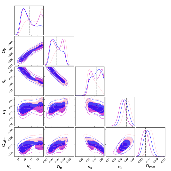
Figure 1: Constraints on cosmological parameters from fits to baseline QSO mocks. The blue contours represent the posteriors when the OuterRim cosmology is taken as the fiducial one, the purple contours (resp. pink) are the posteriors with the BOSS cosmology as the fiducial one, with (resp. without) updating the $k$-range.

Table 2: Constraints on the cosmological parameters in the QSO mock analysis for different configurations. The errors are the 68% marginalized confidence intervals. For $H_{0}$ we report the 95$\%$ lower bound in the last three lines since the error interval reaches the flat prior boundaries we set in the fits. In the line "$\rm C_{fid}=C_{BOSS}~{}\&~{}k=[0.0209,0.3134]~{}\rm h\cdot Mpc^{-1}$", the results are presented as 95$\%$ confidence intervals for the $n_{s}$ and $\Omega_{\rm b}$ parameters because of their bi-modal posteriors.

Configuration	$\Omega_{\rm cdm}$	$\sigma_{8}$	$n_{s}$	$\Omega_{\rm b}$	$H_{0}$
OuterRim cosmology input values	0.2200	0.800	0.963	0.0447	71.00
$\rm Cosmo_{fid}=Cosmo_{OR}$ (baseline)	$0.2234\pm 0.0072$	$0.794\pm 0.012$	$0.986^{+0.016}_{-0.067}$	$0.0412^{+0.0082}_{-0.0012}$	$66.98^{+8.4}_{-0.87}$
$\rm Cosmo_{fid}=Cosmo_{BOSS}$	$0.2297\pm 0.0061$	$0.803\pm 0.011$	$0.9095^{+0.061}_{-0.0099}$	$0.05157^{+0.00060}_{-0.0079}$	$>66.48(95\%)$
$\rm C_{fid}=C_{BOSS}~{}\&~{}k=[0.0209,0.3134]~{}\rm h\cdot Mpc^{-1}$	$0.2183\pm 0.0066$	$0.787\pm 0.011$	$0.898<n_{s}^{\rm fit}<1.020~{}(95\%)$	$0.0374<\Omega_{\rm b}^{\rm fit}<0.0522~{}(95\%)$	$>65.40(95\%)$
alternative mock $\rm C_{fid}=C_{OR}$	$0.226\pm 0.0067$	$0.803^{+0.0089}_{-0.014}$	$0.929^{+0.064}_{-0.011}$	$0.0501^{+0.00064}_{-0.0081}$	$>66.09(95\%)$

Secondly, we perform the same analysis using the BOSS cosmology as the fiducial one (equation 2). This choice is extreme as the BOSS cosmology ($\Omega_{\ rmm}^{\rm BOSS}=0.31$) is significantly different (around 7 times the Planck error on that parameter (Planck Collaboration et al., 2018)) from that of the OuterRim simulation ($\Omega_{\rm m}^{\rm OR}=0.2648$), which induces a dilation of $6.4\%$ and $3.5\%$, of the parallel and perpendicular to the line of sight distances, respectively. In the general case, power spectrum analyses are performed on a specified $k$ range. In different cosmologies, this implies that different physical modes enter the $k$ range under consideration. To overcome this issue, we modify the initial $k$ range (see Table 1) by scaling the limits of the range by a factor that depends on the isotropic distance scales as:

$$k^{\rm BOSS}=k^{\rm OR}\frac{D_{\rm V}^{\rm OR}}{D_{\rm V}^{\rm BOSS}}$$ (23)

where the distances are in $\rm[h^{-1}\cdot Mpc]$ to also account for the different values of $H_{0}$ between the two cosmologies. In the present case, the rescaled range is therefore $k\in[0.0209,0.3134]~{}\rm h\cdot Mpc^{-1}$.

The purple contours and posteriors in figure 1 show the results using the BOSS cosmology and the rescaled $k$-range. For all parameters, the results agree reasonably well with those obtained with the true cosmology of the simulation. The marginalized contour in the $\sigma_{8}-\Omega_{\rm cdm}$ plane shows a slight drift along the line of degeneracy, equivalent to $0.9\%$ and $2.3\%$ shifts for $\sigma_{8}$ and $\Omega_{\rm cdm}$, respectively. This is to be compared to $1.1\%$ and $2.8\%$ without updating the $k$-range. For the other three parameters, $H_{0}$, $\Omega_{\rm b}$ and $n_{s}$, we note that the posteriors are bi-modal. This is likely to be due to the fact that our covariance matrix is approximate since it is based on 100 non-independent realisations. Regardless of this issue, the marginalized 2-dimensional contours of the two analyses nicely overlap for these three parameters and their 68 and 95$\%$ constraints are in agreement.

We also performed this mock analysis using the BOSS cosmology as the fiducial one but with the initial range, $k\in[0.02,0.3]~{}\rm h\cdot Mpc^{-1}$. The pink contours in figure 1 show the corresponding constraints. For $\sigma_{8}$ and $\Omega_{\rm cdm}$, the difference in contours and posteriors due to different $k$ ranges is larger than that due to different fiducial cosmologies. This tends to prove that taking into account the same physical modes is of prime importance to obtain similar constraints. For the other parameters, the updating $k$-range makes the contours and the likelihood profiles closer to those obtained with the true cosmology. Finally, the choice of the fiduciary cosmology may amount to a choice of range in $k$, which should be marginalised in a real data analysis.

4.1.2 Test using different HOD realizations

In previous section, we use the mock2. We test, here, with another HOD prescription called mock4 analysed in the same way, with the OuterRim cosmology as the fiducial one. Results are given in figure 2 and table 2. As for the baseline mocks, the posteriors for mock4 encompass the parameter values expected from the simulation cosmology. As in the previous section, posteriors obtained from the two mocks are in good agreement, especially when considering that the covariance matrix used in the cosmological fit only encompasses noise in the galaxy - halo connection and not cosmic variance (see Section 2.2). For $\sigma_{8}$ and $\Omega_{\rm cdm}$, we note a slight shift of the contour along the degeneracy line, which results in a difference of $1.1\%$ and $1.2\%$ on the two parameter best fit values, respectively.

Summarising, these mock studies demonstrate that the technique proposed here allows to recover the baseline cosmological parameters at $1.5\%$ for $\sigma_{8}$ and $3\%$ for $\Omega_{\rm cdm}$ independently of the chosen fiducial cosmology.

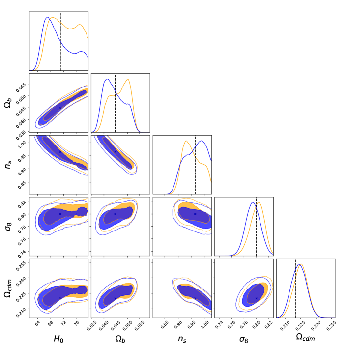
Figure 2: Constraints on cosmological parameters from fits to QSO mocks. The blue (resp. orange) contours represent the analysis posteriors for the baseline (resp. alternative) mocks. The difference being the HOD prescription. All contours assume the OuterRim cosmology as the fiducial one.

4.2 Results on data

The three data samples of section 2.1 were analysed in the same way as mocks. Our main results are shown in figures 3 and 6 and summarised in table 3. We present hereafter combined results as well as results from the individual samples and discuss the impact of priors from external probes.

4.2.1 Combined survey analysis

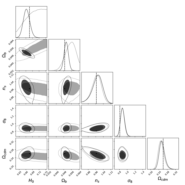
Figure 3: Constraints on the cosmological parameters for the three (e)BOSS surveys used in this analysis. The gray contours represent the posteriors without any external prior, while the black contours assume a prior on $\omega_{b}$ from BBN. The dashed line represents the $\Lambda$CDM Planck best fit.

Table 3: Constraints on cosmological parameters from the analysis of BOSS low-z galaxies, and eBOSS LRG and QSO samples. The errors are the 68% marginalized confidence intervals. $\Omega_{\rm m}$ is a derived parameter.

Data	Priors	$\Omega_{\rm cdm}$	$\sigma_{8}$	$n_{s}$	$\Omega_{\rm b}$	$H_{0}$	$\Omega_{\rm m}$
3 surveys		$0.249^{+0.017}_{-0.011}$	$0.877\pm 0.049$	$0.973\pm 0.054$	$0.0566^{+0.0040}_{-0.0074}$		$0.304^{+0.016}_{-0.010}$
3 surveys	$\omega_{\rm b}$	$0.253^{+0.017}_{-0.010}$	$0.877\pm 0.051$	$0.983\pm 0.056$	$0.0506\pm 0.0022$	$66.1\pm 1.5$	$0.304^{+0.016}_{-0.010}$
3 surveys	$\omega_{\rm b}~{}\&~{}n_{s}$	$0.256\pm 0.010$	$0.869\pm 0.046$	$0.963\pm 0.020$	$0.0503\pm 0.0020$	$66.4\pm 1.4$	$0.308\pm 0.010$
LRG eBOSS + galaxies low-z BOSS		$0.285\pm 0.021$	$0.721^{+0.060}_{-0.028}$	$<0.978(95\%)$	$0.0423^{+0.0090}_{-0.0047}$		$0.328\pm 0.018$
LRG eBOSS + galaxies low-z BOSS	$\omega_{\rm b}$	$0.277\pm 0.018$	$0.738^{+0.056}_{-0.031}$	$<0.988(95\%)$	$0.0483\pm 0.0025$	$67.9\pm 1.8$	$0.324\pm 0.017$
LRG eBOSS + galaxies low-z BOSS	$\omega_{\rm b}~{}\&~{}n_{s}$	$0.265\pm 0.013$	$0.763\pm 0.046$	$0.953\pm 0.019$	$0.0490\pm 0.0024$	$66.9\pm 1.9$	$0.315\pm 0.013$
QSO eBOSS		$0.243^{+0.027}_{-0.014}$	$1.15\pm 0.10$	$1.043^{+0.033}_{-0.075}$	$>0.0472(95\%)$		$0.304^{+0.025}_{-0.015}$
QSO eBOSS	$\omega_{\rm b}$	$0.252^{+0.032}_{-0.014}$	$1.13\pm 0.11$	$1.003^{+0.046}_{-0.100}$	$0.0527\pm 0.0033$	$64.6\pm 2.0$	$0.306^{+0.030}_{-0.015}$
QSO eBOSS	$\omega_{\rm b}~{}\&~{}n_{s}$	$0.267\pm 0.016$	$1.12\pm 0.10$	$0.967\pm 0.021$	$0.0520\pm 0.0031$	$65.1\pm 1.9$	$0.321\pm 0.016$

As shown in figure 3, when no external priors are used (grey contours), we find that $H_{0}$ is very little constrained, as expected in a galaxy clustering analysis. Constraints can be set on $\Omega_{\rm b}$ and $n_{s}$, namely $\Omega_{\rm b}=0.0566^{+0.0040}_{-0.0074}$ and $n_{s}=0.973\pm 0.054$. The uncertainty is an order of magnitude larger than that of the Planck CMB analysis (Planck Collaboration et al., 2018), $\Omega_{\rm b}^{\rm Planck}=0.0493\pm 0.0003$ and $n_{s}^{\rm Planck}=0.965\pm 0.004$. However, galaxy clustering analyses do not usually report any constraint on these parameters. The value of $\Omega_{\rm cdm}=0.249^{+0.017}_{-0.011}$ is within $1\sigma$ of the Planck value. This is true also for the other parameters, except $\sigma_{8}=0.877\pm 0.049$ whose value is $1.4\sigma$ above that of Planck.

Including a prior from the BBN (see section 3.6) on the value of $\omega_{\rm b}=\Omega_{\rm b}\cdot\rm h^{2}$ (black contours), the constraints improve on $H_{0}=66.1\pm 1.5~{}\rm km.s^{-1}.Mpc^{-1}$ and $\Omega_{\rm b}=0.0506\pm 0.0022$. It is however interesting to note that this prior has very little impact on the other constraints e.g. $\Omega_{\rm cdm}=0.253^{+0.017}_{-0.010}$ and $n_{s}=0.983\pm 0.056$ or no impact at all, e.g. $\sigma_{8}=0.877\pm 0.051$ and $\Omega_{\rm m}=0.304^{+0.016}_{-0.010}$.The matter density is identical, only its share between baryons and cold dark matter has varied.

Adding a prior on $n_{s}$ (see section 3.6) to the previous analysis (black contours in figure 6) induces a slight change which remains very small with respect to the statistical error. Altogether, the weak impact of the priors shows that robust cosmological constraints on $\Omega_{\rm m}$ and $\sigma_{8}$ can be obtained without any additional information from external probes on parameters not constrained by galaxy clustering analyses like $n_{s}$ and $\omega_{\rm b}$.

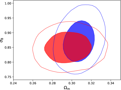
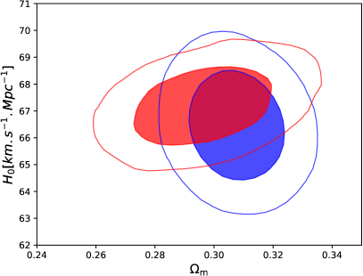
Figure 4: Constraints on the cosmological parameters from this study in blue and from the standard cosmological analysis of (eBOSS Collaboration et al., 2020) in red. In both cases, the same priors are used on $\omega_{\rm b}$ and $n_{s}$. However, it is important to note that we use the eBOSS QSO and LRG surveys as well as the BOSS low-z galaxy survey, while the standard analysis uses all SDSS surveys, which adds the MGS sample, the BOSS high-z galaxies and the eBOSS ELG and Lyman-$\alpha$ surveys. The left-hand plot shows the $\sigma_{8}-\Omega_{\rm m}$ plane, that on the right the $H_{0}-\Omega_{\rm m}$ plane.

In figure 4, we compare our results with those presented in eBOSS Collaboration et al. (2020) based on standard clustering analysis techniques and the $\Lambda$CDM framework. This comparison is done under the same assumptions, i.e. including the same priors on $\omega_{\rm b}$ and $n_{s}$. The contours have similar areas but different orientations and the constraints projected onto $\sigma_{8}$ and $H_{0}$ are stronger with the standard analysis, most probably because of the more extended range in redshift of the extra samples that it includes, as detailed below. The present analysis allows a better constraint on $\Omega_{\rm m}$ despite the differences in terms of number of objects and effective volume. This stronger constraint illustrates the significant gain in precision allowed by a varying template analysis with no compression of the information. To emphasize this, we recall that the present analysis is composed of three samples (BOSS low-z galaxies, eBOSS LRGs and quasars) while the standard analysis is composed, in addition, of the MGS sample, BOSS high-z galaxies, and eBOSS ELG and Lyman-$\alpha$ samples. Therefore, the complete SDSS survey contains 2.5 million objects over a redshift range of $0.07<z<4$ while this analysis includes 1.3 million objects over $0.2<z<2.2$. In addition, the standard analysis uses a consensus between the correlation function and power spectrum analyses, which usually improves errors by $~{}10\%$, while the present study is only carried out in Fourier space.

On the other hand, in this analysis, we do not include errors related to systematic effects. Nevertheless, systematic observational errors have been investigated in individual power spectrum analyses for the informative parameters ($\alpha_{\perp,\parallel}$ and $f\sigma_{8}$) and remain small compared to the statistical error (e.g. $\sigma^{\rm obs}/\sigma^{\rm stat}\sim 0.1$ for quasars). Their addition in quadrature is therefore negligible. Considering the error due to the power spectrum modelling, we remind that the dominant source of error in eBOSS analyses comes from the specification of the cosmology for the model computation. Taking the difference between our mock results obtained with the two different fiducial cosmologies (due to different effective $k$-ranges) as model systematic error leads to $\sigma^{\rm mod}_{\sigma_{8}}=0.012$ and $\sigma^{\rm mod}_{\Omega_{\rm cdm}}=0.007$, which corresponds to $25\%$ and $44\%$ of the statistical error, respectively.

In addition to the present analysis, the full shape two point correlation function of the eBOSS QSO and BOSS DR12 galaxy samples sample were analysed by Semenaite et al. (2021). In their work, they directly constrain the cosmological parameters in configuration space by fitting their modelled two-point correlation function to the data and focus on $h$-independent parameters $\omega_{\rm m}$, $\omega_{\rm DE}$ and $\sigma_{12}$ as proposed by Sánchez (2020). In figure 5, we compare their results with the ones obtained in this work. The three parameters that are recovered from both analyses ($\sigma_{8}$, $\Omega_{\rm m}$ and $n_{s}$) are found to be compatible at the 1 $\sigma$ level, although the samples considered in both analyses are not exactly the same (our work includes the eBOSS LRG sample which is not used in Semenaite et al. (2021) who, however, additionally analyse the measurements from BOSS DR12 high-z sample). In addition to this, there are also differences in modelling the non-linear tracer power spectrum, in particular, Semenaite et al. (2021) use a different model for non-linear clustering predictions as well as a different bias prescription. Finally, the two analyses differ in the choice of priors - firstly, in terms of parameters on which a flat prior is imposed and secondly, in the use of the BBN prior with this analysis employing (when applicable) a significantly tighter Gaussian prior instead of the wider flat informative prior used in Semenaite et al. (2021).

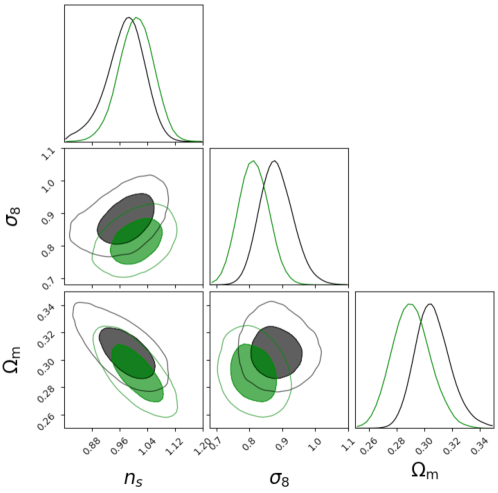
Figure 5: Cosmological constraints on $Omega_{\rm m}$, $\sigma_{8}$ and $n_{s}$. Comparison of our analysis with the BBN-inspired $\omega_{\rm b}$ prior (black contours) to the constraints obtained with an other full shape eBOSS analysis (Semenaite et al., 2021) (green contours).

4.2.2 Single tracer analysis

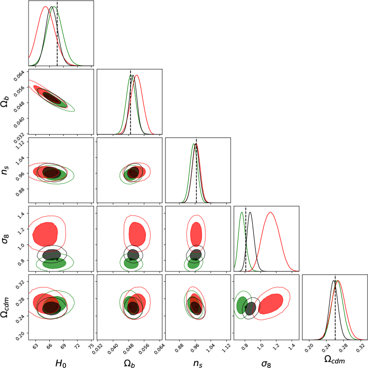
Figure 6: Constraints on the cosmological parameters for the three BOSS surveys by separating the constraints of quasars (in red), and galaxies (in green). The black contours represent the combined posterior of the three surveys. A prior on $\omega_{b}$ and $n_{s}$ have been taken into account. The dashed line represents Planck’s best fit.

In this section, we analyse the low redshift samples (BOSS galaxies and eBOSS LRGs) and the high redshift sample (eBOSS quasars) separately. Figure 6 presents the different contours when including the same priors on $\omega_{\rm b}$ and $n_{s}$ as for the combined analysis. Indeed, as written in table 3, without these priors, $n_{s}$ (resp. $\omega_{b}$) is not constrained better than its range of variation used in the fit to the galaxy (resp. quasar) sample. This may be due to the lower sample size and to the loss of leverage between high and low redshifts in individual analyses compared to the combined one. Including priors in the individual analyses has thus a more important impact than on the combined one. However, this difference is still smaller than the statistical uncertainty.

The posteriors of the low and high redshift analyses agree on $\Omega_{\rm cdm}$ and show a small but not negligible difference on $H_{0}$, $\Omega_{\rm b}$ and $n_{s}$, corresponding to deviations of $0.9\sigma$, $1\sigma$ and $0.7\sigma$, respectively. The constraints on these parameters are also in agreement with Plank results, and so do our derived $\Omega_{\rm m}$ results. On the other hand, the galaxy and quasar analyses differ by $3.6\sigma$ on $\sigma_{8}$. The constraint from the galaxy sample agrees with Planck result ($1.6\sigma$ lower) while that from the quasar sample is $3.1\sigma$ higher. A $2\sigma$ bias with respect to Planck is also visible in the standard analysis (Neveux et al., 2020), when fixing the linear growth rate of structure to the GR expectation. Nevertheless, this discrepancy is reinforced in the present study.

This notably high $\sigma_{8}$ value from high redshift quasars constitutes an unexplained tension with the other data sets used here. This may be due to an unknown or poorly understood systematic effect, physics not explained by the $\Lambda$CDM model, or simply a statistical fluctuation. We did a few tests to check the robustness of this difference. In our framework, we constrain $\sigma_{8}(z=0)$ from the measurement of $f\sigma_{8}(z)$ at $f$ fixed to the value predicted by general relativity at each point of the cosmological parameter space. However, the $\sigma_{8}$ parameter also appears in the amplitude of the power spectrum monopole through the product $b_{1}\sigma_{8}(z)$ (in linear theory).

In figure 7, we show the power spectrum multipoles for the NGC part of the quasar sample (the SGC shows a similar behavior) along with the best fit model for the cases where all tracers (dotted line) or only the quasar sample (solid line) are considered (no external priors). For both fits, there is no constraining power on the value of $h$ and we have set it to $h=0.7$ for the sake of comparison. The monopole is unaffected as a consequence of the $b_{1}\sigma_{8}$ degeneracy previously mentioned. On the other hand, the amplitude of the best fit model for the quadrupole at large scales depends upon the samples considered. Therefore, the difference in $\sigma_{8}$ between the galaxy and quasar fits stems mostly from the amplitude of the quadrupole measured with the eBOSS quasar sample. More data from upcoming surveys should help settle this issue. We verified that the updated scheme to mitigate photometric systematics using the neural network approach proposed by Rezaie et al. (2021) and used in the $f_{\mathrm{NL}}$ analysis of Mueller et al. (2021) had no effect on the power spectrum multipoles in the $k$-range of interest of this work and cannot account for the high value of $\sigma_{8}$. The study presented in Semenaite et al. (2021) also considers the quasar sample alone and their results differ from ours by 1.6 and 1$\sigma$ for $\sigma_{8}$ and $\Omega_{\rm m}$ respectively, which differences in the analysis may explain.

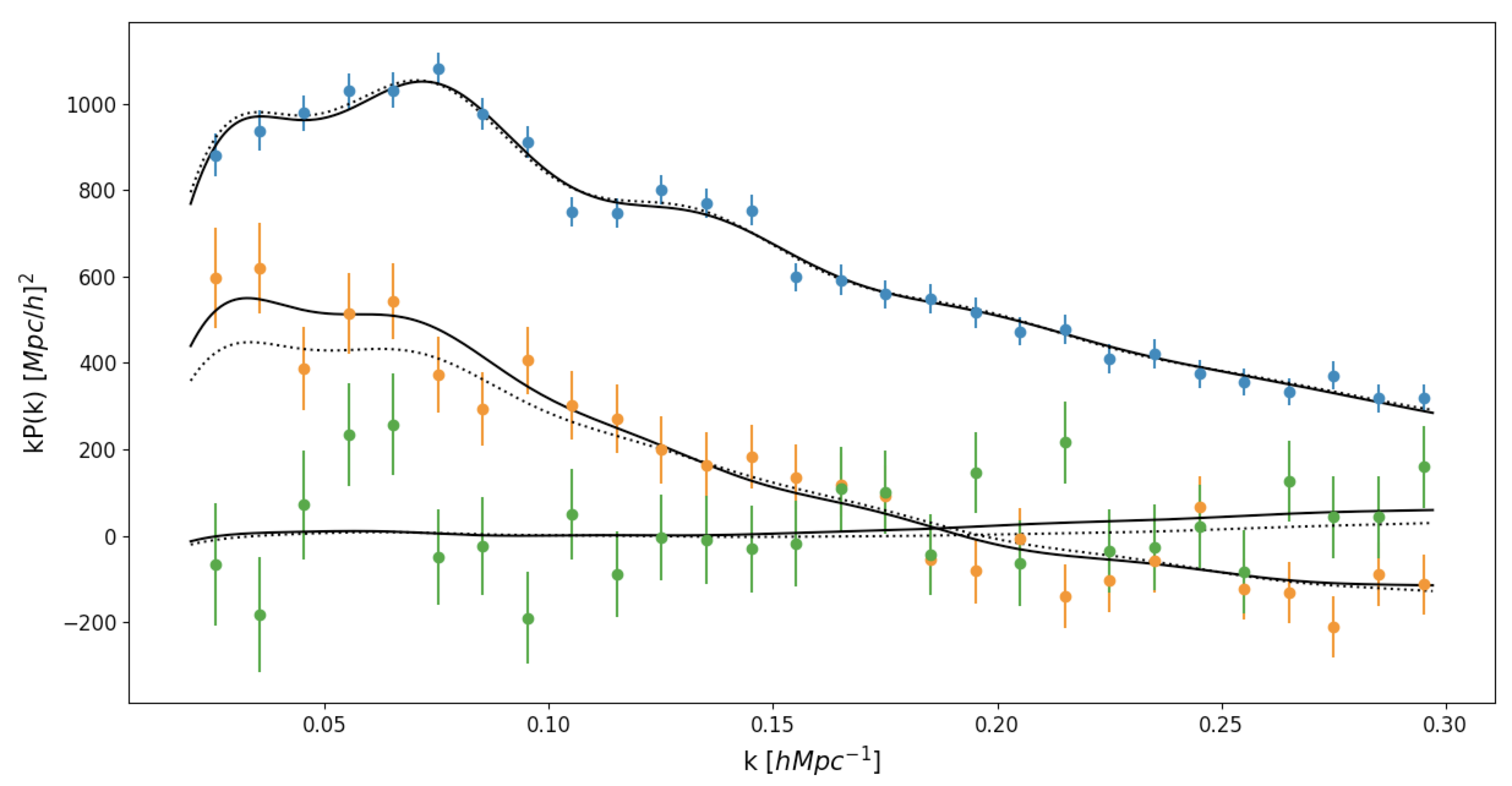
Figure 7: Comparison of the eBOSS NGC data quasar power spectrum multipoles with best fit predictions from the eBOSS quasar sample analysis (solid line) and from the combined analysis (dotted line), both with no external priors. The corresponding best fit cosmologies are $h=0.7,\,\,\Omega_{\rm cdm}=0.252,\,\,\Omega_{b}=0.0640,\,\,\sigma_{8}=1.150,\,\,n_{s}=1.043$ for the solid line and $h=0.7,\,\,\Omega_{\rm cdm}=0.249,\,\,\Omega_{b}=0.0566,\,\,\sigma_{8}=0.877,\,\,n_{s}=0.973$ for the dotted line.

5 Conclusions

We analysed the power spectrum of a subsample of the BOSS and eBOSS data using a TNS model with 2-loop RegPT correction terms. To avoid the fiducial cosmology dependency of the clustering analysis, we built an iterative emulator of the analysis likelihood surface by varying the cosmology of the template model. We fit model power spectra for different cosmologies to the data power spectrum, fixing the dilation scales and the growth rate of structure to their values expected in each tested cosmology and letting the nuisance parameters vary freely. Then, we reconstruct the full likelihood surface in the 5D cosmological parameter space using a Gaussian process algorithm. This technique allows us to fit the cosmological parameters without the standard compression in $f\sigma_{8}$ and scaling parameters $\alpha_{\parallel}$ and $\alpha\perp$ and with minimal power spectrum model computation.

We tested this pipeline on mocks built from the OuterRim N-body simulation and efficiently recovered the five cosmological parameters with good accuracy and precision. Then, we analysed three samples of the SDSS spectroscopic surveys both individually and jointly, namely the BOSS low-z galaxy sample and the eBOSS LRG and QSO samples. The analysis of the QSO sample leads to a $\sigma_{8}$ value significantly different from that predicted from the Planck constraints (Planck Collaboration et al., 2018). This bias is also visible in the standard analysis (Neveux et al., 2020), with a $2\sigma$ deviation from the Planck analysis when fixing the linear growth rate of structure to the GR expectation. Nevertheless, this discrepancy is reinforced in the present study and reaches a $3.1\sigma$ significance. All other parameters are in good agreement with the constraints from the CMB analysis.

The combined likelihood of the three samples allows us to fit $\Omega_{\rm b}$, $n_{s}$, $\Omega_{\rm m}$ and $\sigma_{8}$ without any external prior. We compare our final results with the cosmological analysis of the full SDSS survey; we obtain similar constraints on the $H_{0}$, $\sigma_{8}$ and $\Omega_{\rm m}$ parameters using data sample twice as small. The $\Omega_{\rm m}$ parameter is even better constrained due to the information loss in the compression step in the standard analysis. Such a pipeline that removes the dependence in the fiducial cosmology at all stages of the analysis could be used in future spectroscopic surveys such as DESI or Euclid to reduce the systematic and statistical errors on the cosmological parameters.

Data Availability

The power spectrum, covariance matrices, and resulting likelihoods for cosmological parameters are available via the SDSS Science Archive Server (https://sas.sdss.org/)

References

- Alam et al. (2020) Alam S., et al., 2020, arXiv e-prints, p. arXiv:2007.09004
- Alcock & Paczynski (1979) Alcock C., Paczynski B., 1979, Nature, 281, 358
- Amendola et al. (2018) Amendola L., et al., 2018, Living Reviews in Relativity, 21
- Bautista et al. (2021) Bautista J. E., et al., 2021, MNRAS, 500, 736
- Beutler et al. (2017) Beutler F., et al., 2017, MNRAS, 464, 3409
- Blanton et al. (2017) Blanton M. R., et al., 2017, AJ, 154, 28
- Brieden et al. (2021) Brieden S., Gil-Marín H., Verde L., 2021, ShapeFit: Extracting the power spectrum shape information in galaxy surveys beyond BAO and RSD (arXiv:2106.07641)
- Chen et al. (2021) Chen S.-F., Vlah Z., White M., 2021, A new analysis of the BOSS survey, including full-shape information and post-reconstruction BAO (arXiv:2110.05530)
- Colas et al. (2020) Colas T., d’ Amico G., Senatore L., Zhang P., Beutler F., 2020, Journal of Cosmology and Astroparticle Physics, 2020, 001–001
- Collaboration et al. (2016) Collaboration D., et al., 2016, The DESI Experiment Part I: Science,Targeting, and Survey Design (arXiv:1611.00036)
- Dawson et al. (2013) Dawson K. S., et al., 2013, AJ, 145, 10
- Dawson et al. (2016) Dawson K. S., et al., 2016, AJ, 151, 44
- GPy (2012) GPy since 2012, GPy: A Gaussian process framework in python, http://github.com/SheffieldML/GPy
- Gil-Marín et al. (2020) Gil-Marín H., et al., 2020, MNRAS, 498, 2492
- Grieb et al. (2017) Grieb J. N., et al., 2017, MNRAS, 467, 2085
- Gunn et al. (2006) Gunn J. E., et al., 2006, AJ, 131, 2332
- Habib et al. (2016) Habib S., et al., 2016, New Astron., 42, 49
- Hartlap et al. (2007) Hartlap J., Simon P., Schneider P., 2007, A&A, 464, 399
- Hou et al. (2021) Hou J., et al., 2021, MNRAS, 500, 1201
- Ivanov et al. (2020) Ivanov M. M., Simonović M., Zaldarriaga M., 2020, Journal of Cosmology and Astroparticle Physics, 2020, 042–042
- Kobayashi et al. (2021) Kobayashi Y., Nishimichi T., Takada M., Miyatake H., 2021, arXiv e-prints, p. arXiv:2110.06969
- Kwan et al. (2015) Kwan J., Heitmann K., Habib S., Padmanabhan N., Lawrence E., Finkel H., Frontiere N., Pope A., 2015, ApJ, 810, 35
- Mueller et al. (2021) Mueller E.-M., et al., 2021, arXiv e-prints, p. arXiv:2106.13725
- Myers et al. (2015) Myers A. D., et al., 2015, ApJS, 221, 27
- Neveux et al. (2020) Neveux R., et al., 2020, MNRAS, 499, 210
- Pellejero-Ibañez et al. (2020) Pellejero-Ibañez M., Angulo R. E., Aricó G., Zennaro M., Contreras S., Stücker J., 2020, MNRAS, 499, 5257
- Percival et al. (2014) Percival W. J., et al., 2014, MNRAS, 439, 2531
- Planck Collaboration et al. (2018) Planck Collaboration et al., 2018, arXiv e-prints, p. arXiv:1807.06209
- Prakash et al. (2016) Prakash A., et al., 2016, ApJS, 224, 34
- Rasmussen & Williams (2005) Rasmussen C. E., Williams C. K. I., 2005, Gaussian Processes for Machine Learning (Adaptive Computation and Machine Learning). The MIT Press
- Rezaie et al. (2021) Rezaie M., et al., 2021, MNRAS, 506, 3439
- Saito et al. (2014) Saito S., Baldauf T., Vlah Z., Seljak U., Okumura T., McDonald P., 2014, Phys. Rev. D, 90, 123522
- Sánchez (2020) Sánchez A. G., 2020, Phys. Rev. D, 102, 123511
- Sánchez et al. (2017) Sánchez A. G., et al., 2017, MNRAS, 464, 1640
- Semenaite et al. (2021) Semenaite A., et al., 2021, arXiv e-prints, p. arXiv:2111.03156
- Smee et al. (2013) Smee S. A., et al., 2013, AJ, 146, 32
- Smith et al. (2020) Smith A., et al., 2020, MNRAS, 499, 269
- Tamone et al. (2020) Tamone A., et al., 2020, MNRAS, 499, 5527
- Taruya et al. (2010) Taruya A., Nishimichi T., Saito S., 2010, Phys. Rev. D, 82, 063522
- Taruya et al. (2012) Taruya A., Bernardeau F., Nishimichi T., Codis S., 2012, Physical Review D, 86
- Tröster et al. (2020) Tröster T., et al., 2020, A&A, 633, L10
- Zhai et al. (2019) Zhai Z., et al., 2019, ApJ, 874, 95
- Zhang & Cai (2021) Zhang P., Cai Y., 2021, BOSS full-shape analysis from the EFTofLSS with exact time dependence (arXiv:2111.05739)
- de Mattia & Ruhlmann-Kleider (2019) de Mattia A., Ruhlmann-Kleider V., 2019, J. Cosmology Astropart. Phys., 2019, 036
- de Mattia et al. (2021) de Mattia A., et al., 2021, MNRAS, 501, 5616
- d’ Amico et al. (2020) d’ Amico G., Gleyzes J., Kokron N., Markovic K., Senatore L., Zhang P., Beutler F., Gil-Marín H., 2020, Journal of Cosmology and Astroparticle Physics, 2020, 005–005
- eBOSS Collaboration et al. (2020) eBOSS Collaboration et al., 2020, arXiv e-prints, p. arXiv:2007.08991