Photodissociation dynamics of N${}_{3}^{+}$

Abstract

The photodissociation dynamics of N${}_{3}^{+}$ excited from its ${}^{3}\Sigma_{\rm g}^{-}$ ground to the first excited singlet and triplet states is investigated. Three dimensional potential energy surfaces for the ¹A^′, ¹A^′′, and ³A^′ electronic states, correlating with the ${}^{1}\Delta_{\rm g}$ and ${}^{3}\Pi_{\rm u}$ states in linear geometry, for N${}_{3}^{+}$ are constructed using high level electronic structure calculations and represented as reproducing kernels. The reference ab initio energies are calculated at the MRCI+Q/aug-cc-pVTZ level of theory. For following the photodissociation dynamics in the excited states, rotational and vibrational distributions $P(v^{\prime})$ and $P(j^{\prime})$ for the N₂ product are determined from vertically excited ground state distributions. Due to the different shapes of the ground state ³A${}^{{}^{\prime\prime}}$ PES and the excited states, appreciable angular momentum $j^{\prime}\sim 60$ is generated in the diatomic fragments. The lifetimes in the excited states extend to at least 50 ps. Notably, results from sampling initial conditions from a thermal ensemble and from the Wigner distribution of the ground state wavefunction are comparable.

I Introduction

Many important processes occurring in the earth’s atmosphere involve nitrogen-containing species as it is the most abundant element in the medium. Among these are charge transfer processes such as N(⁴S) + N${}_{2}^{+}$(X${}^{2}\Sigma_{\rm g}^{+}$) $\leftrightarrow$ N⁺(³P) + N₂(X${}^{1}\Sigma_{\rm g}^{+}$) that proceed via the formation of the N${}_{3}^{+}$ radical cation. An early study utilized the complete active space self-consistent field (CASSCF) approach and multireference configuration interaction method (MRCI) to calculate vertical excitation energies and specify the collinear dissociation paths of the electronically excited states of the N${}_{3}^{+}$ ion.Bennett et al. (1996) Given its importance in a variety of atmospheric reactions, the photodissociation dynamics of the $\textrm{N}_{3}^{+}$ ion warrants a detailed investigation.

Reactions involving N${}_{3}^{+}$ are relevant in air plasmas at elevated temperatures. Under such conditions, N${}_{3}^{+}$ can serve as an N⁺ donor to species such as NO, O₂, SO₂, N₂O, CO₂, or CO.de Petris et al. (2006); Midey, Miller, and Viggiano (2004); Dunkin et al. (1971); Popovic et al. (2004) Thus, decomposition of N${}_{3}^{+}$ into N⁺ + N₂ is of particular relevance in view of the general reaction scheme N${}_{3}^{+}$ + M $\rightarrow$ NM⁺ + N₂ with subsequent decomposition of NM⁺. Species of particular importance that are formed through N⁺ transfer reactions are NCO⁺ (N${}_{3}^{+}$ + CO $\rightarrow$ NCO⁺ + N₂) and NCO${}_{2}^{+}$ (N${}_{3}^{+}$ + CO₂ $\rightarrow$ NCO${}_{2}^{+}$ + N₂).de Petris et al. (2006) Furthermore, N${}_{3}^{+}$ together with N${}_{4}^{+}$ have been suggested to be the most abundant nitrogen-containing ions in the lower atmosphere of Titan where the N${}_{3}^{+}$ ion drives several reactions involving CH₄, C₂H₂ or C₂H₄ through N⁺ atom transfer.Anicich et al. (2000)

Photodissociation reactions are induced by the absorption of one or more photons by a chemical species which can then disintegrate to form products. In a typical photolytic reaction, a reactant ABC with internal energy $E_{\rm int}$ absorbs a photon with energy $h\nu$ to form a transient activated complex [ABC]* which can undergo several types of primary photochemical processes followed by secondary processes. One possible outcome is the subsequent dissociation of [ABC]* into A+[BC]* where the product BC molecule is formed in a variety of excited quantum states whose population depends on the available energy and the dynamical details of the dissociation process

$${\rm ABC}\overset{h\nu}{\rightarrow}{\rm[ABC]}^{*}\rightarrow{\rm A+[BC]*}$$ (1)

A dynamics study for a chemical reaction usually begins with the generation of an accurate potential energy surface (PES) for the species. For the system of interest, 1- and 2-dimensional sections through the 3-dimensional PESs for the ground and electronically excited states have been previously determined at different levels of theory.Chambaud et al. (1994); Bennett et al. (1996); Tarroni and Tosi (2004) In addition, one- and 3-dimensional PESs for cyclic-N${}_{3}^{+}$ were determined,Dillon and Yarkony (2007); Babikov, Mozhayskiy, and Krylov (2006); Mozhayskiy, Babikov, and Krylov (2006) and the vibrational levels up to $\sim 2$ eV were computed.Babikov, Mozhayskiy, and Krylov (2006); Mozhayskiy, Babikov, and Krylov (2006) Finally, ab initio MD simulations for the vibrational spectroscopy of linear and cyclic N${}_{3}^{+}$ have been carried out.Jolibois, Maron, and Ramirez-Solis (2009) These studies were concerned with the electronic spectroscopy and the lower vibrational states on the ground state PES. However, a full-dimensional PES for the electronic ground state has only become available recently.Koner et al. (2020)

The construction of high-dimensional PESs is a challenging problem for which machine learning-based approaches like neural networks or kernel-based methods have found wide applicability in recent times.Unke and Meuwly (2017); Manzhos and Carrington (2021); Unke et al. (2021); Meuwly (2021) One such method, rooted in the theory of reproducing kernel Hilbert spaces (RKHSs),Ho and Rabitz (1996) is suitable for obtaining reliable PESs. For this, a training set of data is generated using electronic structure calculations which is then used to "train" the algorithm to produce a continuous surface by interpolating smoothly between the data points. Here this ’training set’ constitutes the total electronic energy evaluated at various configurations using high-level electronic structure calculations. This method was utilized in previous work for the construction of an accurate PES for the ground state of $\textrm{N}_{3}^{+}$ at the multi reference configuration interaction (MRCI) level of theory.Koner et al. (2020) A similar methodology has been followed for the construction of high quality PESs for other triatomic species such as the [CNO] system,Koner, Bemish, and Meuwly (2018) N${}_{3}^{-}$,Salehi, Koner, and Meuwly (2019) and NO₂.San Vicente Veliz et al. (2020) In the current work the focus is on those excited states of the N${}_{3}^{+}$ cation which are expected to be accessible during photoexcitation. Photodissociation reactions of the N${}_{3}^{+}$ ion involve transitions between the ${}^{3}\Sigma_{\rm g}^{-}$ (³A^′′ in bent geometry) ground state and energetically accessible excited states. The ¹A^′, ¹A^′′ and ³A^′ excited states of N${}_{3}^{+}$ are expected to play a role in dynamical processes owing to their energetic proximity to the ground state (${}^{3}\Sigma_{\rm g}^{-}$).

The present work is structured as follows. First, the methods are presented. Next, the quality of the PESs is discussed and the results from the dynamics simulations for photoexcitation to the ³A${}^{{}^{\prime}}$ and the two singlet states are reported. Next, simulations starting from sampling the Wigner distribution of the ground state wavefunction are compared with the more conventional thermal initial conditions. Finally, the results are discussed and conclusions are drawn.

II Methods

First, the methods for generating and representing the potential energy surfaces are summarized. Following this, the QCT and quantum simulations for studying N${}_{3}^{+}$$\rightarrow$N₂+N⁺ photodissociation are described.

II.1 The N${}_{3}^{+}$ Potential Energy Surfaces

The 3-dimensional PESs for the ¹A^′, ¹A^′′, and ³A^′ states of N${}_{3}^{+}$ were computed at the MRCISDWerner and Knowles (1988); Knowles and Werner (1988)/aug-cc-pVTZDunning (1989) level of theory with the Davidson quadruples correctionLanghoff and Davidson (1974) (MRCISD+Q) based on a CASSCFWerner and Knowles (1985); Knowles and Werner (1985); Werner and Meyer (1980); Kreplin, Knowles, and Werner (2019) reference wave function. Also, the 2d-PES at $r_{\rm NN}=2.25$ a₀ (see below) for the $2^{3}$A${}^{{}^{\prime\prime}}$ state was determined. All electronic structure calculations were carried out using the Molpro 2019.1 program.Werner et al. (2012, 2019) The active space for CASSCF included the full valence space. State-averaged (SA) calculations were carried out using 8 states in total, including the two lowest states of the ³A^′′ (ground state), ¹A^′, ¹A^′′, and ³A^′ symmetries, respectively.

For the electronic structure calculations, the grid was defined in Jacobi coordinates $(R,r,\theta)$ whereby $r$ is the separation between nitrogen N1 and N2, $R$ is the distance between N3 and the center of mass of N1 and N2, and $\theta$ is the angle between $\vec{r}$ and $\vec{R}$; see Figure 2. The grid includes distances $r\in[1.55,4.00]$ a₀, $R\in[1.5,10.0]$ a₀, and $\theta\in[0,180^{\circ}]$ from a $7$-point Legendre quadrature. The products of the photodissociation reaction of N${}_{3}^{+}$ are N₂ and N⁺. Thus, the energy of the system for $E(R\rightarrow\infty,r)$ is the sum of the energies of the dissociation products. In the following, the "zero" of energy is set to this value according to $V(R,r,\theta)=E(R,r,\theta)-E(R\rightarrow\infty,r)$.

For the dynamics simulations the energies on the grid are most conveniently represented in a way that allows evaluation of energies and analytical gradients for arbitrary conformations. Here, a reproducing kernel Hilbert space (RKHS) representation is employed.Ho and Rabitz (1996); Unke and Meuwly (2017) According to the representer theoremSchölkopf, Herbrich, and Smola (2001), a function $f(\mathbf{x})$ for which values $f(\mathbf{x_{i}})$ are given for arguments $\mathbf{x}$, can always be approximated as a linear combination

$$f(\mathbf{x})\approx\widetilde{f}(\mathbf{x})=\sum_{i=1}^{N}\alpha_{i}K(\mathbf{x},\mathbf{x}_{i}).$$ (2)

Here, $K(\mathbf{x},\mathbf{x^{\prime}})$ is a kernel function and $\alpha_{i}$ are coefficients to be determined from matrix inversion. If the inner product $\langle\phi(\mathbf{x}),\phi(\mathbf{x^{\prime}})\rangle$ can be written as $K(\mathbf{x},\mathbf{x^{\prime}})$, the function is called a reproducing kernel of a Hilbert space $\mathcal{H}$.Berlinet and Thomas-Agnan (2011)

Here, reciprocal power decay kernel polynomials are used for the radial coordinates. For the $R-$coordinate kernel functions ($k^{[n,m]}$) with smoothness $n=2$ and asymptotic decay $m=4$

$$k^{[2,4]}(x,x^{\prime})=\frac{2}{15}\frac{1}{x^{5}_{>}}-\frac{2}{21}\frac{x_{<}}{x^{6}_{>}},$$ (3)

are employed, while $n=2$ and $m=6$ is used for the $r$ dimension

$$k^{[2,6]}(x,x^{\prime})=\frac{1}{14}\frac{1}{x^{7}_{>}}-\frac{1}{18}\frac{x_{<}}{x^{8}_{>}},$$ (4)

In both expressions, $x_{>}$ and $x_{<}$ are the larger and smaller values of $x$ and $x^{\prime}$, respectively. Such a kernel smoothly decays to zero giving the correct long-range behavior for atom-diatom type interactions. For the angle $\theta$ a Taylor spline kernel is used:

$$k^{[2]}(z,z^{\prime})=1+z_{<}z_{>}+2z^{2}_{<}z_{>}-\frac{2}{3}z^{3}_{<},$$ (5)

Here, $z_{>}$ and $z_{<}$ are the larger and smaller values of $z$ and $z^{\prime}$, respectively, and $z$ is defined as

$$z=\frac{1-{\rm cos}\theta}{2},$$ (6)

with $z\in[0,1]$. Combination of the three 1-dimensional kernels leads to

$$K({\bf{x}},{\bf{x}}^{\prime})=k^{[2,4]}(R,R^{\prime})k^{[2,6]}(r,r^{\prime})k^{[2]}(z,z^{\prime}),$$ (7)

where, ${\bf{x}},{\bf{x}}^{\prime}$ are $(R,r,z)$ and $(R^{\prime},r^{\prime},z^{\prime})$, respectively. The coefficients $\alpha_{i}$ and the RKHS representation of the PES are evaluated by using a computationally efficient toolkit.Unke and Meuwly (2017)

The global reactive PES for each excited electronic state is constructed by smoothly connecting the three PESs for the three symmetry-equivalent reaction channels using a switching function,

$$V(\mathbf{r})=\sum_{j=1}^{3}\omega_{j}(r_{j})V_{j}(\mathbf{r})$$ (8)

where the switching function $\omega_{j}$ has an exponential form,

$$\omega_{i}(r)=\frac{e^{-(r_{i}/\rho_{j})^{2}}}{\sum_{j=1}^{3}e^{-(r_{j}/\rho_{j})^{2}}}$$ (9)

Such a mixing using normalized weights is akin to that used in multi surface reactive MD.Nagy, Yosa Reyes, and Meuwly (2014); Schmid et al. (2018) The mixing parameters $\rho_{j}$ for each channel are obtained using least squares fitting. For the ³A${}^{{}^{\prime\prime}}$ ground state of $\textrm{N}_{3}^{+}$, the switching parameters are $\rho=(0.65,0.65,0.65)$ a₀.Koner et al. (2020) The root mean squared error between the two sets of data is $\sim 0.8$ kcal/mol (0.034 eV) over the entire range of reference energies considered. Similarly, reactive PESs were constructed for the ¹A${}^{{}^{\prime}}$, ¹A${}^{{}^{\prime\prime}}$ and ³A${}^{{}^{\prime}}$ excited states. For the ¹A${}^{{}^{\prime}}$ state, the switching parameters are $\rho=(1.0,1.0,1.0)$ a₀ with an RMSE of $\sim 0.6$ kcal/mol (0.026 eV). For the ¹A${}^{{}^{\prime\prime}}$ state, the switching parameter was $\rho=(1.03,1.03,1.03)$ a₀ with an RMSE of $\sim 0.6$ kcal/mol (0.026 eV) and for the ³A${}^{{}^{\prime}}$ state, a switching parameter of $\rho=(0.75,0.75,0.75)$ a₀ yielded an RMSE of $\sim 0.06$ kcal/mol (0.003 eV) for the global reactive PES.

II.2 Quasi-Classical Trajectory Simulations

The QCT simulations used in the present work have been extensively described in the literature.Truhlar and Muckerman (1979); Henriksen and Hansen (2011); Koner et al. (2016); Koner, Bemish, and Meuwly (2018) Here, Hamilton’s equations of motion are solved using a fourth-order Runge-Kutta numerical method. The time step was $\Delta t=0.05$ fs which guarantees conservation of the total energy and angular momentum.

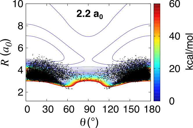
Figure S1: 500000 configurations generated on the ${}^{3}\textrm{A}^{{}^{\prime\prime}}$ (ground) state at 1000 K are projected on the ${}^{3}\textrm{A}^{{}^{\prime}}$ PES of $\textrm{N}_{3}^{+}$. This set of phase space points are used as initial conditions for photodissociation. See text for discussion.

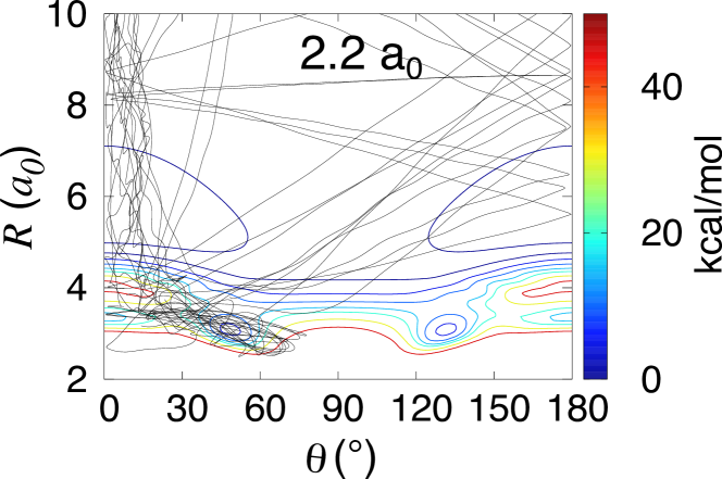
Figure S2: Photodissociating trajectories on the ${}^{3}\textrm{A}^{{}^{\prime}}$ excited state of $\textrm{N}_{3}^{+}$ at 1000 K. Initial conditions generated on the ${}^{3}\textrm{A}^{{}^{\prime\prime}}$ (ground) state at 1000 K are vertically excited to the ${}^{3}\textrm{A}^{{}^{\prime}}$ state PES and propagated up to a final time of 50 ps. The N–N diatomic separation is fixed at $r=2.2$ a₀ for the underlying PES in the graph.

For the photodissociation simulations, structures in the vicinity of the ³A^′′ ground state PES and velocities were generated by drawing from a Maxwell-Boltzmann distribution at temperatures between 500 K and 3000 K. Each of the 500000 initial conditions was propagated for 50 ps on the ground state PES and the final positions and velocities were saved. For a view of the ensemble of structures; see Figure S1. Following this, the entire population is projected vertically to the excited state PESs. Trajectories on the excited states are run until dissociation into products occurs or for a maximum of 50 ps. Configurations initially located around the ground state minima land in the vicinity of a potential well when projected onto the ${}^{3}\textrm{A}^{{}^{\prime}}$ PES. Subsequent trajectories are initially confined in the region around the minima before dissociating into products. Examples for photodissociating trajectories from initial velocities generated at 1000 K on the ${}^{3}\textrm{A}^{{}^{\prime}}$ PES are shown in Figure S2.

The product ro-vibrational states are determined following semiclassical quantization. Since the ro-vibrational states of the product diatom are continuous numbers, the states need to be assigned to integer quantum numbers for which a Gaussian binning (GB) scheme was used. For this, Gaussian weights centered around the integer values with a full width at half maximum of 0.1 were used.Bonnet and Rayez (1997, 2004); Koner et al. (2016) It is noted that using histogram binning (HB) was found to give comparable results for a similar system.Koner, Bemish, and Meuwly (2018)

II.3 Bound Vibrational States for Electronically Excited States of N${}_{3}^{+}$

The vibrational energy levels supported by the singlet excited state PESs are computed using the DVR3D suite of codes.Tennyson et al. (2004) For this, the nuclear time-independent Schrödinger equation is solved over a discrete grid in Jacobi coordinates $(R,r,\theta)$. In this method, the three internal coordinates are treated in a discrete variable representation (DVR). The angular coordinate is represented as a 56-point DVR based on Gauss-Legendre quadrature and the radial coordinates utilise a DVR based on Gauss-Laguerre quadratures with 72 points along $R$ and 48 points along $r$. The angular basis functions are Legendre polynomials and the radial basis functions are Laguerre polynomials. For the ³A${}^{{}^{\prime}}$ PES, the states predissociate due to the double-well structure of the surface; see Figure 1.

The optimized Morse parameters for the grid in $r$ for the ¹A^′ state are $r_{e}=2.50$ a₀, $D_{e}=0.32$ $E_{\rm h}$ and $\omega_{e}=0.006$ $E_{\rm h}$, and $R_{e}=3.4$ a₀, $D_{e}=0.15$ $E_{\rm h}$ and $\omega_{e}=0.0015$ $E_{\rm h}$ for $R$. With these parameters the $r$ grid for ¹A^′ extends from 1.49 to 3.46 a₀ while the $R$ grid ranges from 1.20 to 5.51 a₀. The corresponding Morse parameters for the ¹A^′′ state are $r_{e}=2.45$ a₀, $D_{e}=0.32$ $E_{\rm h}$ and $\omega_{e}=0.0065$ $E_{\rm h}$ along $r$ and $R_{e}=3.5$ a₀, $D_{e}=0.15$ $E_{\rm h}$ and $\omega_{e}=0.0015$ $E_{\rm h}$ for $R$. The $r$ grid is from 1.48 to 3.36 a₀ while the $R$ grid spans 1.30 to 5.61 a₀. For determination of the rotational levels, the body-fixed $z-$axis is oriented along $R$. The corresponding vibrational wave functions obtained as amplitudes over a discrete grid in Jacobi coordinates are transformed to symmetric $(R_{\rm N1N2}+R_{\rm N2N3})/\sqrt{2}$), asymmetric $(R_{\rm N1N2}-R_{\rm N2N3})/\sqrt{2}$) and bending coordinates $\angle$ N1N2N3 using a Gaussian kernel-based interpolation method. Here, the triatomic is denoted as N1–N2–N3. This transformation allows the approximate assignment of the wavefunctions using quantum numbers obtained by counting the nodal planes along each coordinate.

III Results

III.1 The Potential Energy Surfaces of the Excited States

In the following the quality and topology of the excited state PESs determined in the present work is described. The $1^{3}$A${}^{{}^{\prime\prime}}$ ground state PES, correlating with the ${}^{3}\Sigma_{\rm g}^{-}$ state in linear geometry and dissociating to N${}^{+}(^{3}{\rm P})$+N${}_{2}({\rm X}^{1}\Sigma_{\rm g}^{+})$, was already discussed in earlier work.Koner et al. (2020) Next up in energy are the ¹A${}^{{}^{\prime}}$ and ¹A${}^{{}^{\prime\prime}}$ states (see left panel in Figure 1), which are degenerate for $\theta=0$, correlate with the ${}^{1}\Delta_{\rm g}$ state and dissociate to N${}^{+}(^{1}{\rm D})$+N${}_{2}({\rm X}^{1}\Sigma_{\rm g}^{+})$. Upon bending away from the linear structure the degeneracy is lifted and two states - ¹A${}^{{}^{\prime}}$ and ¹A${}^{{}^{\prime\prime}}$ - emerge as is shown in Figure 1 middle and right panels. The overall shapes of the two PESs for the ¹A states follow that of the ³A${}^{{}^{\prime\prime}}$ ground state PES.

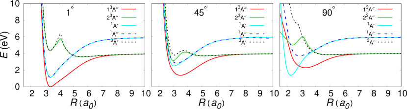
Figure 1: One dimensional sections of the three dimensional PESs of the ground and excited states of N${}_{3}^{+}$. All cuts are taken at $r=2.25$ $a_{0}$ and the values of the angle $\theta$ are indicated at the top of each plot. For linear N${}_{3}^{+}$ ($\theta=0$) the ground state (³A${}^{{}^{\prime\prime}}$) correlates with the ${}^{3}\Sigma_{\rm g}^{-}$ state, the two ¹A states (¹A${}^{{}^{\prime}}$ and ¹A${}^{{}^{\prime\prime}}$, degenerate in linear geometry) with the ${}^{1}\Sigma_{\rm g}^{+}$ state, and ³A${}^{{}^{\prime}}$ and $2^{3}$A${}^{{}^{\prime\prime}}$ correlate with the ${}^{3}\Pi_{\rm u}$ state.

At yet higher energy and most relevant for the photodissociation dynamics considered later, are the ³A${}^{{}^{\prime}}$ and $2^{3}$A${}^{{}^{\prime\prime}}$ states which correlate with the ${}^{3}\Pi_{\rm u}$ state in linear geometry. Both states dissociate to N${}^{+}(^{3}{\rm P})$+N${}_{2}({\rm X}^{1}\Sigma_{\rm g}^{+})$, i.e. they have the same asymptote as the $1^{3}$A${}^{{}^{\prime\prime}}$ (${}^{3}\Sigma_{\rm g}^{-}$) ground state. The ³A${}^{{}^{\prime}}$ state has a double minimum PES with a first minimum at $R=3.365$ a₀ which is higher in energy than the corresponding N₂(${}^{1}\Sigma_{\rm g}^{+}$)+N⁺(³P) asymptote by 0.328 eV and separated from it by a barrier of 2.351 eV in the linear configuration; see Figure 1. This double well structure of the PES disappears upon bending of the N${}_{3}^{+}$ molecule and leads to a repulsive PES for a T-shaped structure, see right hand panel in Figure 1. Thus, ${}^{3}\Pi_{\rm u}$ $\leftarrow$ ${}^{3}\Sigma_{\rm g}^{-}$ excitation of linear N${}_{3}^{+}$ from the ground to the excited state is expected to lead to pronounced angular dynamics, also because the structure with $\theta=45^{\circ}$ in the region of the excitation ($R\in[3\cdots 4]$ a₀) is lower in energy than for the linear conformation, see middle panel Figure 1. For the $2^{3}$A${}^{{}^{\prime\prime}}$ state the 1d-cuts resemble the ³A${}^{{}^{\prime}}$ state for the linear and $\theta=45^{\circ}$ geometries. For the T-shaped conformation there is a local minimum at $R=2.384$ a₀. For $R>3$ a₀ the ³A${}^{{}^{\prime}}$ and $2^{3}$A${}^{{}^{\prime\prime}}$ states overlap again. Because the geometry of the ³A${}^{{}^{\prime\prime}}$ ground state is linear, photoexcitation to the triplet states is expected to primarily populate regions around $\theta=0$.

The vertical excitation energies for the ${}^{1}\Delta_{\rm g}$$\leftarrow$${}^{3}\Sigma_{\rm g}^{-}$ and the ${}^{3}\Pi_{\rm u}$$\leftarrow$${}^{3}\Sigma_{\rm g}^{-}$ transitions have been determined or estimated from experiments.Dyke et al. (1982) For the ${}^{1}\Delta_{\rm g}$$\leftarrow$${}^{3}\Sigma_{\rm g}^{-}$ transition the excitation energy estimated from photoelectron spectroscopy is 1.13 eV, and for the ${}^{3}\Pi_{\rm u}$$\leftarrow$${}^{3}\Sigma_{\rm g}^{-}$ transition a laser spectroscopy study yielded an excitation energy of 4.54 eV.Friedmann et al. (1994) From the present calculations and for the linear configuration with $r=2.25$ a₀, these two excitation energies are 1.13 eV and 4.35 eV, respectively; see Figure 1. These results agree favourably with experiments. Earlier MRCI calculations reported transition energies of 1.30 eV and 4.48 eV and 1.13 eV and 4.28 eV when Davidson corrections are included.Bennett et al. (1996)

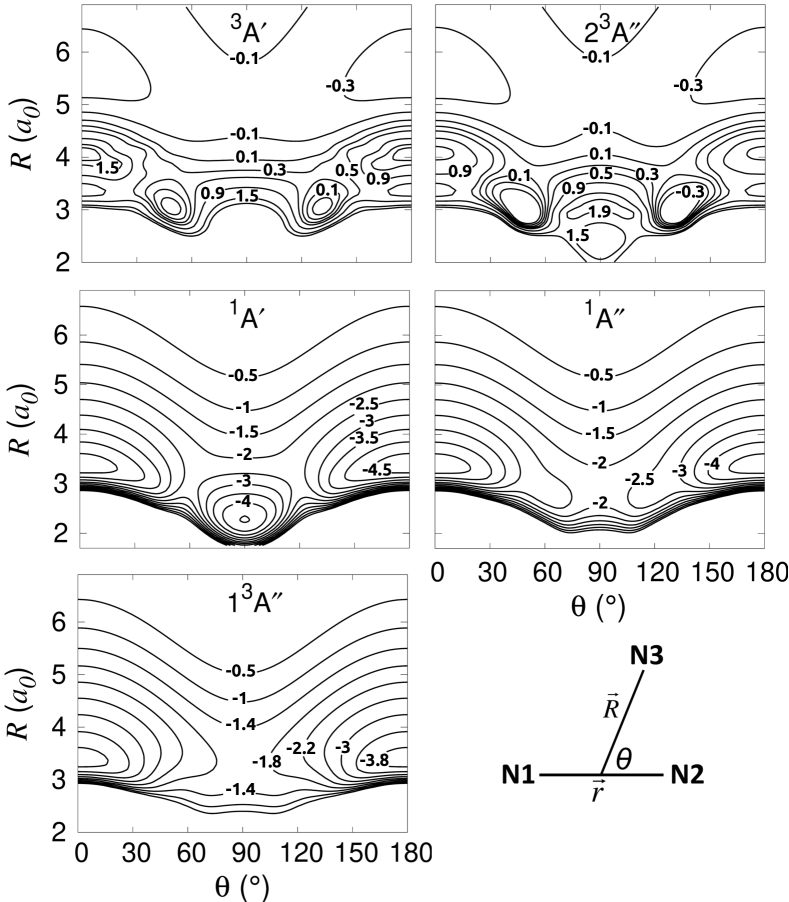
Figure 2: Two-dimensional contour plots for the PESs of the $1^{3}$A${}^{{}^{\prime\prime}}$ ground state (${}^{3}\Sigma_{\rm g}^{-}$ for linear N${}_{3}^{+}$, lower left), the two ¹A states (¹A${}^{{}^{\prime}}$, middle left and ¹A${}^{{}^{\prime\prime}}$ middle right) corresponding to the ${}^{1}\Delta_{\rm g}$ state in the linear structure, and the two ³A states (³A${}^{{}^{\prime}}$ middle left and $2^{3}$A${}^{{}^{\prime\prime}}$ middle right) correlating with the ${}^{3}\Pi_{\rm u}$ state. In all panels the N1–N2 diatomic separation is fixed at $r=2.25$ a₀. The asymptote for the triplet states is $E_{\rm N_{2}}+E_{\rm N^{+}(^{3}P)}$ and for the singlet states it is $E_{\rm N_{2}}+E_{\rm N^{+}(^{1}D)}$. All energies are reported in eV. The bottom right panel shows the Jacobi coordinates $(R,r,\theta)$ used for describing the 3-dimensional PESs for N${}_{3}^{+}$. The vector $\vec{r}$ is the N1–N2 separation, $\vec{R}$ is the separation between N3 and the center of mass of N1–N2, and $\theta$ is the angle between the two distance vectors.

The RKHS representations for the four electronically excited states are provided in Figure 2. The minimum energy structure of the ³A${}^{{}^{\prime\prime}}$ ground state (Figure 2 bottom left) is 3.99 eV below the N₂(${}^{1}\Sigma_{\rm g}^{+}$)+N⁺(³P) limit with a barrier of $2.28$ eV for interconversion between the two equivalent linear minima. The ³A${}^{{}^{\prime}}$ state (Figure 2 upper left) has minima at $\theta=49.8^{\circ}(130.8^{\circ})$, 0.493 eV above the N₂(${}^{1}\Sigma_{\rm g}^{+}$)+N⁺(³P) dissociation limit and local minima at $\theta=0^{\circ}(180^{\circ})$, 0.328 eV above the same asymptote. It also contains local maxima at $\theta=0^{\circ}(180^{\circ})$ with height 2.351 eV above the same asymptote. For the $2^{3}$A${}^{{}^{\prime\prime}}$ state, a 2-dimensional PES at fixed N1-N2 separation $r_{\rm NN}=2.25$ a₀ was determined on the same $(R,\theta)$ grid as for all other states. The RKHS representation is illustrated in the upper right panel of Figure 2. For the linear geometry $\theta=0^{\circ}$ the ³A${}^{{}^{\prime}}$ and $2^{3}$A${}^{{}^{\prime\prime}}$ PESs are degenerate and associated with the ${}^{3}\Pi_{\rm u}$ state (see Figure 1), with a slight difference around $R\sim 4$ a₀. For nonlinear geometries the two states split as was already found in earlier electronic structure calculations.Tarroni and Tosi (2004) Overall, the topography of the ³A${}^{{}^{\prime}}$ and $2^{3}$A${}^{{}^{\prime\prime}}$ states which both derive from the ${}^{3}\Pi_{\rm u}$ state of linear N${}_{3}^{+}$ are similar except for a local minimum in the T-shaped geometry for the $2^{3}$A${}^{{}^{\prime\prime}}$ state. This minimum is separated by a barrier of $\sim 1.6$ eV from the minimum at $\theta\sim 45^{\circ}$. As the ³A${}^{{}^{\prime}}$ and $2^{3}$A${}^{{}^{\prime\prime}}$ PESs are similar for $\theta\lesssim 45^{\circ}$ and photoexcitation from the ground state primarily populates this region of the PES, the photodissociation dynamics on the ³A${}^{{}^{\prime}}$ and $2^{3}$A${}^{{}^{\prime\prime}}$ surfaces are expected to be comparable. Sampling of the local minimum around $\theta\sim 90^{\circ}$ on the $2^{3}$A${}^{{}^{\prime\prime}}$ state following photoexcitation is unlikely as this local, T-shaped minimum is separated by a barrier exceeding 1 eV from the region with $\theta\leq 45^{\circ}$.

The ¹A${}^{{}^{\prime}}$ and ¹A${}^{{}^{\prime\prime}}$ states derive from the ${}^{1}\Delta_{\rm g}$ state of linear, centrosymmetric N${}_{3}^{+}$. The ¹A${}^{{}^{\prime}}$ state (Figure 2 middle left) has two minima, a local one at $\theta=0^{\circ}(180^{\circ})$, 4.824 eV below the N₂(${}^{1}\Sigma_{\rm g}^{+}$)+N⁺(¹D) asymptote and the global one at $\theta=90^{\circ}$ which is 5.090 eV below the same asymptote. The barrier between the two minima is 2.425 eV above the respective asymptote. The ¹A${}^{{}^{\prime\prime}}$ state (Figure 2 middle right) features a minimum at linear positions 4.824 eV below the N₂(${}^{1}\Sigma_{\rm g}^{+}$)+N⁺(¹D) asymptote. The barrier between the two symmetrical minima is 2.229 eV above the respective asymptote. The locations and energies of all the critical points are summarized in Table 1.

Table 1: Minima and transition states for the 3-dimensional ground and excited PESs of N${}_{3}^{+}$ considered in the present work. The PESs are represented in Jacobi coordinates. All interatomic distances are in Bohr ($a_{0}$) and angles are in degree. Energies are reported in eV with respect to the $\textrm{N}+\textrm{N}+\textrm{N}^{+}(^{3}\textrm{P})$ asymptote for the triplet states and $\textrm{N}+\textrm{N}+\textrm{N}^{+}(^{1}\textrm{D})$ asymptote for the singlet states. The electronic states are labelled for both, ${\rm D}_{\infty\rm h}$ and ${\rm C_{s}}$ symmetries. Results for the $2^{3}$A^′′ state are not reported because only a 2-dimensional PES was determined.

		$R$	$r$	$\theta$	$E$
	MIN1	3.38	2.25	0.0	-13.05
${}^{3}\Sigma_{\rm g}^{-}$/3A′′	MIN2	3.38	2.25	180.0	-13.05
	TS1	3.37	2.14	90.0	-10.90
	MIN1	2.18	2.51	90.0	-14.10
	MIN2	3.38	2.25	0.0	-13.83
${}^{1}\Delta_{\rm g}$/1A′	MIN3	3.38	2.25	180.0	-13.83
	TS1	2.84	2.34	61.0	-11.35
	TS2	2.84	2.34	119.0	-11.35
	MIN1	3.38	2.25	0.0	-13.83
${}^{1}\Delta_{\rm g}$/1A′′	MIN2	3.38	2.25	180.0	-13.83
	TS1	2.97	2.18	90.0	-11.27
	MIN1	3.01	2.41	49.2	–9.50
	MIN2	3.01	2.41	130.8	–9.50
	MIN3	3.36	2.24	0.0	–8.69
${}^{3}\Pi_{\rm u}$/3A′	MIN4	3.36	2.24	180.0	–8.69
	TS1	3.36	2.32	21.0	–8.51
	TS2	3.36	2.32	159.0	–8.51
	TS3	5.06	2.09	90.0	–9.56

As a verification for the quality of the RKHS representation, electronic energies at additional grid points, which are not part of the training set, are evaluated from ab initio calculations and evaluation of the RKHS. The correlation between the reference MRCI+Q energies and their representation as a RKHS is given in Figure 3. For the ¹A${}^{{}^{\prime}}$ state, energies at 400 additional grid points are calculated and a correlation coefficient of 0.99969 is obtained, demonstrating the high accuracy of the RKHS-represented PESs. Similarly, validation sets of 530 and 315 grid points for the ¹A${}^{{}^{\prime\prime}}$ and ³A${}^{{}^{\prime}}$ states yield correlation coefficients 0.99998 and 0.99978, respectively.

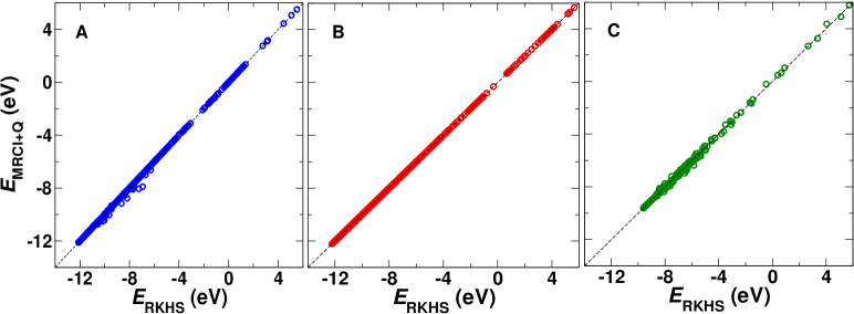
Figure 3: Correlation between ab initio and RKHS energies for the ¹A${}^{{}^{\prime}}$ (panel A), ¹A${}^{{}^{\prime\prime}}$ (panel B), and ³A${}^{{}^{\prime}}$ (panel C) excited states of N${}_{3}^{+}$. The respective correlation coefficients for the three PES are $R^{2}=0.99969$ for ¹A${}^{{}^{\prime}}$, $R^{2}=0.99998$ for ¹A${}^{{}^{\prime\prime}}$ and $R^{2}=0.99978$ for the ³A${}^{{}^{\prime}}$ state.

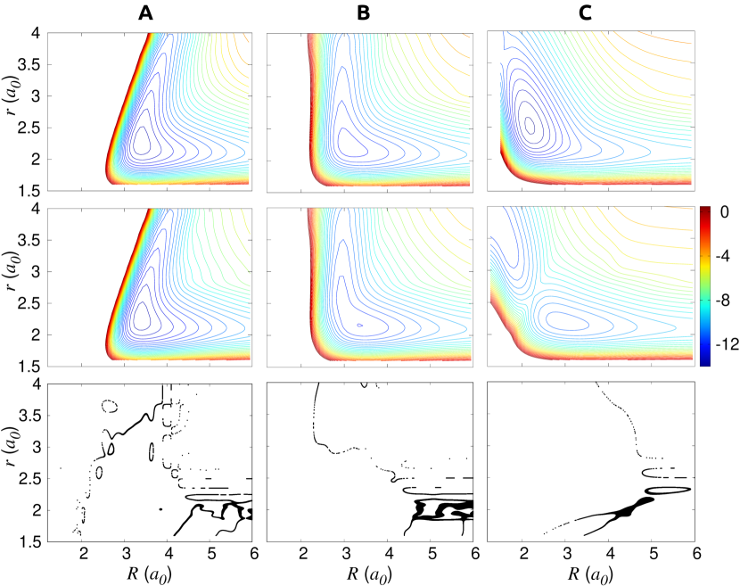
Figure S3: Contour plots $V(R,r)$ for the singlet excited states of N${}_{3}^{+}$ and the crossing points between them. Configurations are considered on the crossing seam if the energy difference between the two PESs is within $10^{-5}$ eV. The surfaces are shown for three different values of the Jacobi angle $\theta=0.01^{\circ}$ (panel A), $\theta=45^{\circ}$ (panel B), and $\theta=90^{\circ}$ (panel C). The top and middle rows show the ¹A${}^{{}^{\prime}}$ and ¹A${}^{{}^{\prime\prime}}$ PESs respectively while the bottom row shows the points at which the respective PESs cross each other. All energies are in eV.

The crossing seams between the two singlet electronic states, which are degenerate in the linear configuration, are reported in Figure S3. The geometries at which the two states cross were stored whenever the energy difference between the ¹A${}^{{}^{\prime}}$ and ¹A${}^{{}^{\prime\prime}}$ states was smaller than $10^{-5}$ eV for a given geometry. Crossing seams are shown for three different values of the angle $\theta$. Thus, for the excited vibrational states, there is a possibility of nonadiabatic transitions between the ¹A${}^{{}^{\prime}}$ and ¹A${}^{{}^{\prime\prime}}$ states.

III.2 ${}^{3}\Pi_{\rm u}$$\leftarrow$${}^{3}\Sigma_{\rm g}^{-}$ Photodissociation Dynamics

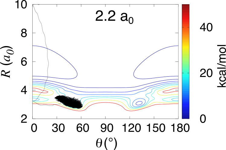
Figure S4: A trajectory with an excited state lifetime of $\sim 17$ ps projected on the ${}^{3}\textrm{A}^{{}^{\prime}}$ PES. The simulations were carried out at 1000 K. The 2d-PES is shown for $r=2.2$ a₀.

The photodissociation dynamics on the excited ³A^′ state is studied by evaluating the vibrational and rotational state distributions of the products. The product final state distributions from initial conditions generated at the different temperatures are shown in Figure 4. Vertical photoexcitation of a thermalized ensemble of molecules on the ground electronic state results in their promotion to the lowest energy vibrational level of the excited state. As temperature increases higher $v^{\prime}$ values become populated gradually with $v^{\prime}_{\rm max}=4$. In Figure 4 the final rotational distributions at all temperatures are also shown. Only the results for the most populated $v^{\prime}=0$ state are presented. The excited state population is distributed over a wide range of rotational states with the peak of the distribution shifting to higher values as temperature increases. Examples for photodissociating trajectories at 1000 K on the ${}^{3}\textrm{A}^{{}^{\prime}}$ PES are shown in Figure S2. Configurations initially located around the ground state minima land in the vicinity of a potential well when projected onto the ${}^{3}\textrm{A}^{{}^{\prime}}$ PES. Several of these trajectories are confined in the region around the minima for a few vibrational periods before dissociating into products. Several trajectories also arrive at the potential barrier near $\theta\sim 0^{\circ}$ and undergo dissociation immediately. Note that only trajectories resulting from initial conditions with $\theta=0^{\circ}$ to $90^{\circ}$ are shown in the figure. Trajectories initialized from $\theta=90^{\circ}$ to $180^{\circ}$ follow similar dynamical paths on account of the symmetry of the PES. The distribution of lifetimes $P(\tau)$ of the $\textrm{N}_{3}^{+}$ complex in Figure 4 indicates that a large fraction of the trajectories leads to photodissociation within 5 ps after excitation. However, there is also a number of trajectories with considerably longer lifetimes. Figure S4 shows one such trajectory at 1000 K with a lifetime of 17 ps.

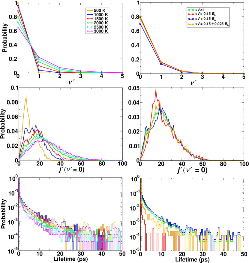
Figure 4: Photodissociation dynamics on the ³A^′ PES. Left column: Product vibrational (top) and rotational (middle) state distributions and lifetime distributions (bottom) from simulations started with velocities from Maxwell-Boltzmann distributions at different temperatures on the ground state PES and vertical excitation to the excited state. Right column: Product vibrational and rotational state distributions and lifetime distributions from simulations started with velocities from Maxwell-Boltzmann distributions at 2000 K on the ground state PES. The analysis is carried out for different criteria for $\Delta V=V_{\rm es}-V_{\rm gs}$ as specified in the figure legend and in the text. For comparison, the product state distributions when all initial conformations undergo photoexcitation are shown in blue. In all cases, the resulting trajectories are propagated for a maximum time of 50 ps or until dissociation, whichever is earlier.

Up to this point the entire ground state population was projected onto the excited state PES and the dynamics was followed. In other words, it was assumed that the resonance condition, $h\nu=E_{\rm photon}=E_{\rm es}-E_{\rm gs}=\Delta V$, is always fulfilled. Here, $h\nu$ is the energy of the incoming photon and $E_{\rm gs}$ and $E_{\rm es}$ are the energies of the molecule in the ground and excited states, respectively. However, experimentally typically only a fraction of the population is promoted from the lower to the upper state. Such processes constitute a subset of the trajectories discussed so far and are discussed next. An examination of the PESs corresponding to $\theta\approx 0^{\circ}$ in Figure 1 reveals that the difference in energies between the respective minima on the ³A${}^{{}^{\prime}}$ and ³A${}^{{}^{\prime\prime}}$ states is $\Delta V\approx 4$ eV indicating that with initial conditions in the vicinity of the ground state minimum, molecules would require $\sim 4$ eV energy for the transition to the excited state. Hence, the following different cases are considered : (1) $\Delta V>0.15E_{\rm h}$ ($\approx 4$ eV), (2) $\Delta V<0.15$ $E_{\rm h}$, and (3) $\Delta V=0.15\pm 0.025$ $E_{\rm h}$. The results for the ensuing dynamics from trajectories sampled from initial conditions at 2000 K are shown in Figure 4 (right hand column). The respective distributions when all trajectories are photoexcited are also shown on the same graphs for comparison. The energy difference for Case (1) corresponds to a photon wavelength $\lambda<310$ nm.

If only the low-energy part of the distribution is promoted to the excited state ($\Delta V<0.15$ $E_{\rm h}$) the population of the vibrationally excited state in the product state is slightly smaller than for the other three cases. Conversely, excitation with $\Delta V>0.15$ $E_{\rm h}$ leads to a maximum value $j_{\rm max}^{\prime}$ which is somewhat lower than for the remaining cases. The most pronounced differences arise for the lifetimes on the excited state, which depend on what fraction of the ground state distribution is excited. For high energy excitation ($\Delta V>0.15$ $E_{\rm h}$) lifetimes are strongly clustered on the picosecond time scales with a maximum lifetime of 20 ps. For near-resonant excitation ($\Delta V=0.15\pm 0.025$ $E_{\rm h}$) lifetimes on the several 10 ps time scale are more probable, extending out to 50 ps. Excitation of the low-energy part of the ensemble (green) leads to a higher probability for longer lifetimes but the shape of the distribution is similar to that for exciting the entire ground state population (blue).

III.3 ${}^{1}\Delta_{\rm g}$$\leftarrow$${}^{3}\Sigma_{\rm g}^{-}$ Photodissociation Dynamics

Formally, the ³A^′ $\rightarrow$ ¹A^′ and ³A^′ $\rightarrow$ ¹A^′′ transitions involve a change of multiplicity and are forbidden, and therefore expected to be weak. Nevertheless, it is of interest to consider how the final state distributions depend on the different topographies of the underlying PESs by comparing final state distributions from transitions to the ³A^′′, ¹A^′, and ¹A^′′ states, respectively; see Figure 2.

For the linear geometry the ¹A${}^{{}^{\prime}}$ and ¹A${}^{{}^{\prime\prime}}$ PESs are degenerate. As the middle row of Figure 2 shows, the most notable difference between the two singlet states is the presence of a potential well near $\theta=90^{\circ}$ for the ¹A${}^{{}^{\prime}}$ state. Thus, a trajectory starting with $\theta\approx 0^{\circ}$ or $180^{\circ}$ on the ¹A${}^{{}^{\prime\prime}}$ state remains confined in the neighbourhood of the potential wells until sufficient energy has accumulated along the dissociative coordinate(s) to decompose whereas a trajectory with similar initial conditions but propagating on the ¹A${}^{{}^{\prime}}$ state PES may potentially travel towards $\theta=90^{\circ}$ on account of the presence of a minimum at this position. However, the barrier to reach this minimum is $\sim 2.75$ eV (see Table 1) which is too high to be overcome at the conditions studied here. Nevertheless, away from the global minimum the shapes of the two singlet PESs differ somewhat.

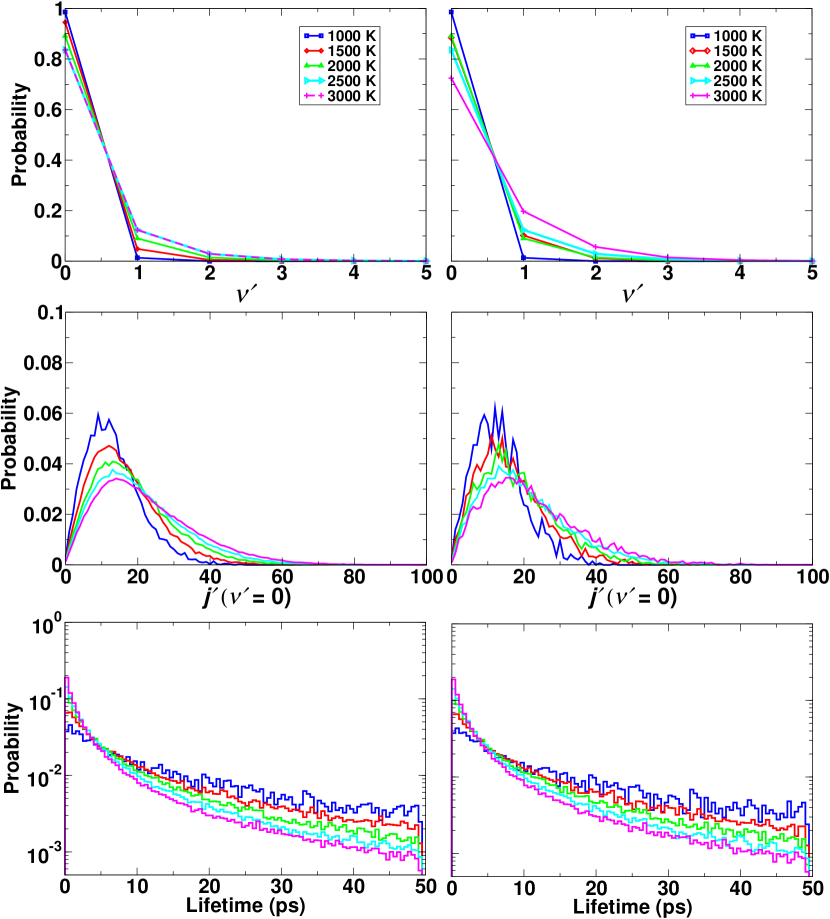
Figure 5: Photodissociation dynamics for the singlet excited state PESs of $\textrm{N}_{3}^{+}$. Product vibrational and rotational state distributions and lifetime distributions at different temperatures for photodissociation of N${}_{3}^{+}$ on the ${}^{1}\textrm{A}^{{}^{\prime}}$ (left column) and ${}^{1}\textrm{A}^{{}^{\prime\prime}}$ (right column) excited states. Thermalized initial conditions are generated on the ground state at the respective temperatures and propagated on the excited state PES. In all cases, the resulting trajectories are propagated for a maximum time of 50 ps or until dissociation, whichever is earlier.

The final state vibrational distributions from dynamics on the ¹A${}^{{}^{\prime}}$ PES are dominated by population of $v^{\prime}=0$ with maximum population of $v^{\prime}=1$ at higher temperatures only reaching $\sim 10$ %, see left column in Figure 5. For the rotational state distributions $P(j^{\prime})$ corresponding to $v^{\prime}=0$ the maxima occur between $j^{\prime}=10$ and $j^{\prime}=13$, depending on temperature. Short lifetimes ($\sim 1$ ps) on the excited state PES before dissociation are about one order of magnitude more probable than lifetimes of $\sim 50$ ps at 1000 K. This changes to a difference of 2 orders of magnitudes at 3000 K with short lifetimes beoming much more probable.

For photodissociation from the ¹A${}^{{}^{\prime\prime}}$ state (Figure 5 right column) excitation of $v^{\prime}=1$ reaches up to 20 % for higher temperatures. This is a clear difference compared with vibrational products dissociating from the ¹A${}^{{}^{\prime}}$ state. For the rotational distributions corresponding to $v^{\prime}=0$ the maxima also shift progressively to higher $j^{\prime}$ values with increasing temperature but the maxima occur at somewhat higher rotational quantum numbers compared with dissociation by populating the ¹A${}^{{}^{\prime}}$ state. Finally, for the ¹A${}^{{}^{\prime\prime}}$ state at $T\sim 1000$ K, short lifetimes are about one order of magnitude more probable than long lifetimes. Short lifetimes become even more probable as temperature increases. These aspects are similar for dynamics on the ¹A${}^{{}^{\prime}}$ state.

Overall, photodissociation on the two singlet states follows comparable patterns although details in the final state rotational distributions indicate that the anisotropy of the ¹A${}^{{}^{\prime\prime}}$ state PES differs somewhat from that of the ¹A${}^{{}^{\prime}}$ PES, see middle row of Figure 2. Conversely, photodissociation from the ³A^′ state leads to more pronounced population of vibrationally excited states $v^{\prime}>0$, in particular at higher temperatures, and the rotational distributions $P(j^{\prime};v^{\prime}=0)$ appear broader with the maxima of the distributions shifted to higher values of $j^{\prime}$ compared with photodissociation from the two singlet states. This can be related to the flatter PES along the angular coordinate in the ³A^′ state compared with the two singlet states which leads to sampling of larger angular distortions and to increased torque upon photodissociation.

IV Discussion and Conclusion

So far, the photodissociation dynamics of the N${}_{3}^{+}$ ion in the lowest singlet and triplet excited states was followed based on QCT simulations. Consistent with the shape differences between the ${}^{3}\Sigma_{\rm g}^{-}$ ground state PES and the three electronically excited PESs high rotational excitations in $j^{\prime}$ after photodissociation are found. To further corroborate this finding, simulations starting from sampling the Wigner distributionWigner (1932); Weinbub and Ferry (2018) of the ${}^{3}\Sigma_{\rm g}^{-}$ ground state wavefunction were also carried out. The Wigner function $f_{W}(\Gamma)$ related to a three dimensional wavefunction in Jacobi coordinates $\Psi(R,r,\theta)$ is

$$f_{W}(\Gamma)=(\pi\hbar)^{-3}\int ds_{R}ds_{r}ds_{\theta}\quad e^{2i(Ps_{R}+ps_{r}+Ps_{\theta})/\hbar}\\ \times\Psi^{*}(R+s_{R},r+s_{r},\theta+s_{\theta})\times\Psi(R-s_{R},r-s_{r},\theta-s_{\theta})$$ (10)

with $\Gamma=(R,r,\theta,P,p,P_{\theta})$. Initial conditions for photodissociation are generated by sampling the probability distribution $f_{W}(\Gamma)$ in Eq.10 using Metropolis Monte Carlo importance sampling. Here, $\Psi(R,r,\theta)$ is the ground state wavefunction for the ${}^{3}\textrm{A}^{{}^{\prime\prime}}$ PES. The collection of initial conditions generated on the ground state PES in this manner represent the quantum wavepacket which is then projected onto the excited state as before and the dynamics is followed from QCT simulations.

The resulting final state distributions are shown in Figure 6. The quantum ground state is 1421 cm^-1 above the minimum energy of the PES, corresponding to 2000 K. Final state distributions from classical trajectories sampled from the Wigner distribution follow closely those from classical simulations with initial conditions at low temperature (500 K). Since “temperature” is not a meaningful physical quantity for such small systems,Boltachev and Schmelzer (2010) $T$ is rather more a label to distinguish how initial conditions were generated for ensembles which are increasingly energized. Given this, it is encouraging to see that final state distributions from classical trajectories starting from two very different strategies to generate initial conditions are consistent with one another.

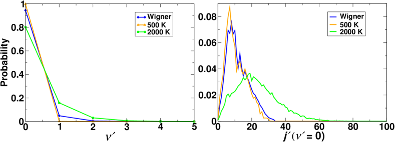
Figure 6: Photodissociation dynamics for the ${}^{3}\textrm{A}^{{}^{\prime}}$ excited state of N${}^{+}_{3}$ with trajectories started from configurations obtained by sampling the Wigner distribution (blue) corresponding to the quantum ground state on the ${}^{3}\Sigma_{\rm g}^{-}$ state and from QCT simulations at 500 K (orange) and 2000 K (green), respectively. Final vibrational (left) and rotational (right) state distributions are shown. The results are for vertical excitation from the ground to the ${}^{3}\Pi_{\rm u}$/${}^{3}\textrm{A}^{{}^{\prime}}$ excited state.

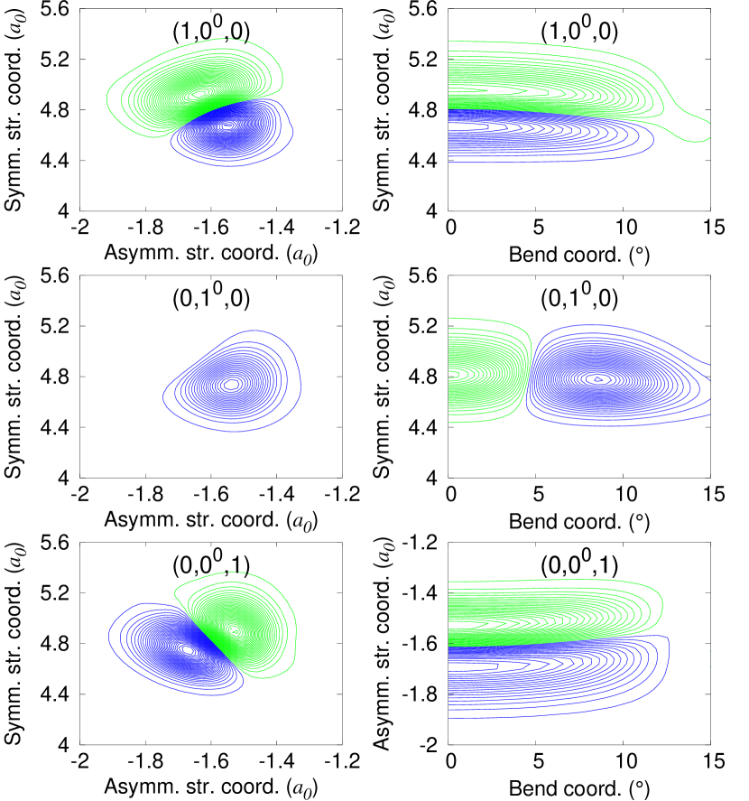
Figure S6: Wave functions for the fundamentals of ${}^{1}\textrm{A}^{{}^{\prime\prime}}$ excited state of $\textrm{N}_{3}^{+}$ from DVR3D calculations. The states are indicated by the labels ($\nu_{1}\nu_{2}^{l}\nu_{3}$).

To corroborate the pronounced coupling of the intermolecular modes it is also useful to consider the lower quantum bound states for the different PESs. For this, the 3-dimensional time-independent Schrödinger equation was solved for the lowest bound vibrational states on the the two lowest singlet electronically excited PESs, neglecting Renner-Teller coupling. The zero point vibrational energies for the ¹A${}^{{}^{\prime}}$ and ¹A${}^{{}^{\prime\prime}}$ PESs are 1809 cm^-1 and 1707 cm^-1, respectively. Fundamentals are at 1019 cm^-1 and 1281 cm^-1 for the $v_{3}$ antisymmetric stretch, at 1496 cm^-1 and 1241 cm^-1 for the $v_{1}$ symmetric stretch, and at 1041 cm^-1 and 814 cm^-1 for the $v_{2}$ bending vibration. This compares with fundamentals at 1096 cm^-1, 774 cm^-1, and 395 cm^-1 for the $v_{1}$, $v_{3}$, and $v_{2}$ vibrations on the ${}^{3}\Sigma_{\rm g}^{-}$ ground state PES. The higher vibrational states (combination bands and overtones) are approximately assigned using vibrational quantum numbers based on node counting; the results are reported in Table 2. It must be noted that the assignments are rather approximate due to the anharmonicities and strong couplings prevalent among the vibrational levels of the excited states. This can also be seen for the representative wavefunctions for lower energy levels of the ¹A${}^{{}^{\prime}}$ and ¹A${}^{{}^{\prime\prime}}$ states shown in Figures S5 and Figure S6 respectively. Similar calculations for the triplet state ³A${}^{{}^{\prime}}$ were not performed as it predissociates and requires full scattering calculations, which are outside the scope of the present work.

Table 2: Lower bound states (in cm^-1 above the ground state) for the singlet electronically excited states of N${}^{+}_{3}$. The bound states are assigned to vibrational quantum numbers $v_{1}$ (symmetric stretch), $v_{2}$ (bend), and $v_{3}$ (antisymmetric stretch) by node-counting; see Figures S5 and S6 for examples. The labels are only approximate due to strong coupling. The angular momentum quantum number is $l$.

$v_{1}v_{2}^{l}v_{3}$	${}^{1}\textrm{A}^{\prime}$	$v_{1}v_{2}^{l}v_{3}$	${}^{1}\textrm{A}^{\prime\prime}$
0 $0^{0}$ 1	1018.8	0 $1^{1}$ 0	813.6
0 $1^{1}$ 0	1040.9	1 $0^{0}$ 0	1241.2
1 $0^{0}$ 0	1496.1	0 $0^{0}$ 1	1281.1
0 $0^{0}$ 2	2033.1	0 $2^{0}$ 0	1627.4
0 $1^{1}$ 1	2048.9	1 $1^{1}$ 0	2064.1
0 $2^{0}$ 0	2063.3	0 $1^{1}$ 1	2068.3
1 $1^{1}$ 0	2490.8	0 $0^{0}$ 2	2435.7
1 $0^{0}$ 1	2492.7	0 $3^{1}$ 0	2446.8
2 $1^{1}$ 1	2512.8	2 $0^{0}$ 0	2455.3
2 $2^{0}$ 0	2825.9	1 $0^{0}$ 1	2601.5
2 $0^{0}$ 0	2979.7	0 $2^{0}$ 1	2853.4
0 $0^{0}$ 3	3041.1	1 $2^{0}$ 0	2885.1
1 $0^{0}$ 3	3481.9	2 $1^{1}$ 0	3242.4

The current work investigates the photodissociation dynamics of the N${}_{3}^{+}$ ion for the three lowest electronically excited states. For this, an ensemble of initial conditions is generated on the ground state PES and projected onto each of the excited states. For the ³A${}^{{}^{\prime}}$ PES, it is found that $P(v^{\prime})$ essentially does not depend on how the excitation takes place. Excitation of the entire ground state population gives a similar $P(v^{\prime})$ compared with near-resonant excitation or when only the high-energy part of the ground state distribution is excited. This is somewhat different for $P(j^{\prime})$ for which excitation of the high-energy population yields slightly lower $j_{\rm max}^{\prime}$ compared with the other three excitation schemes. Using initial conditions sampled from the Wigner distribution of the ground state wavefunction to initiate the dynamics on the ³A${}^{{}^{\prime}}$ excited state leads to comparable final state distributions $P(v^{\prime})$ and $P(j^{\prime})$ as do simulations started from initial conditions generated at 500 K. Product state distributions for the $2^{3}$A${}^{{}^{\prime\prime}}$ state are expected to be similar to those from excitation to the ³A${}^{{}^{\prime}}$ state due to the similar shape of the PES for $\theta\leq 45^{\circ}$. Even for larger bending angles the two PESs are quite similar except for a high-lying T-shaped minimum for short $R-$separations which is, however, energetically inaccessible.

The present work reports testable results for experiments from classical and semiclassical dynamics on accurate, high-level potential energy surfaces for this important ion. It is hoped that the predictions spur experimental efforts to better characterize the photodissociation dynamics of N${}_{3}^{+}$. This will be of particular relevance to atmospheric and interstellar chemistry.

Supporting Information

The supporting information reports the initial conditions on the ground state PES, individual photodissociating trajectories, the crossing seams between the singlet PES, and wavefunctions for the fundamentals on the two singlet PESs.

Data Availability Statement

All information necessary to construct the potential energy surfaces is available at https://github.com/MMunibas/N3p_PESs.

Supporting Information: Photodissociation Dynamics of N${}_{3}^{+}$

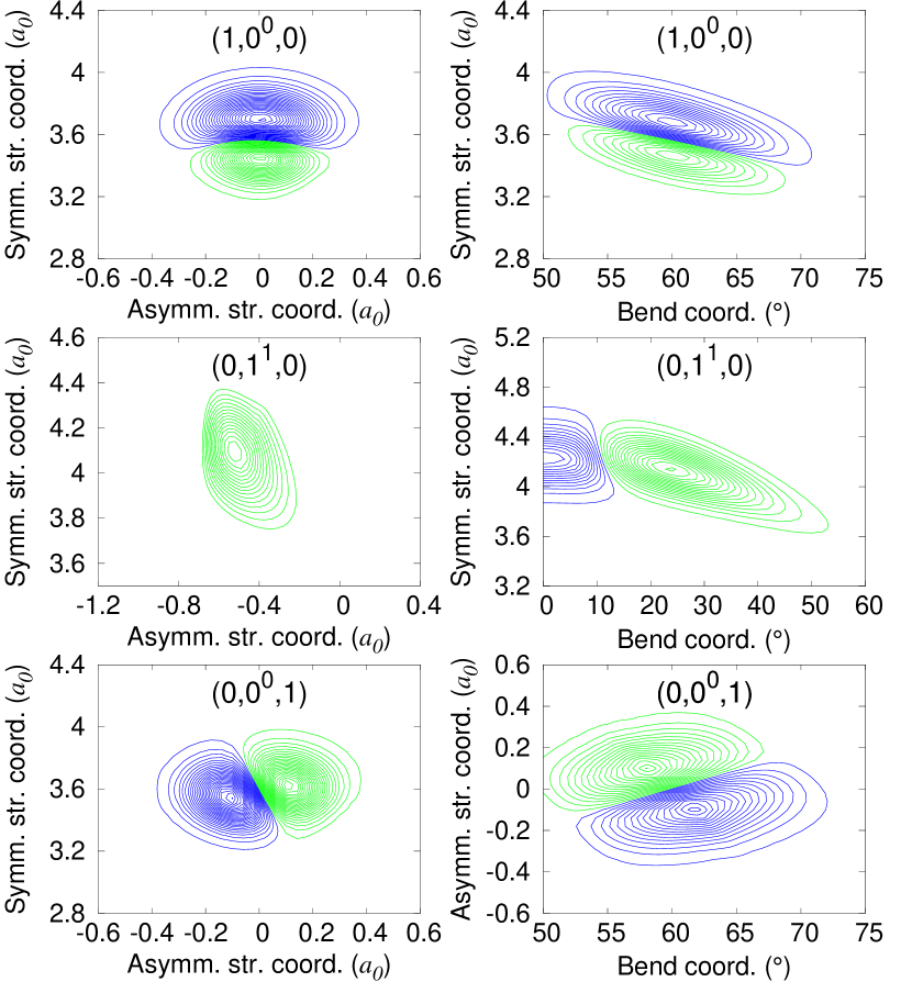
Figure S5: Wave functions for the fundamentals of ${}^{1}\textrm{A}^{{}^{\prime}}$ excited state of $\textrm{N}_{3}^{+}$ from DVR3D calculations. The states are indicated by the labels ($\nu_{1}\nu_{2}^{l}\nu_{3}$).

References

- Bennett et al. (1996) F. R. Bennett, J. P. Maier, G. Chambaud, and P. Rosmus, Chem. Phys. 209, 275 (1996).
- de Petris et al. (2006) G. de Petris, A. Cartoni, G. Angelini, O. Ursini, A. Bottoni, and M. Calvaresi, ChemPhysChem 7, 2105 (2006).
- Midey, Miller, and Viggiano (2004) A. Midey, T. Miller, and A. Viggiano, J. Chem. Phys. 121, 6822 (2004).
- Dunkin et al. (1971) D. Dunkin, F. Fehsenfeld, A. Schmeltekopf, and E. Ferguson, J. Chem. Phys. 54, 3817 (1971).
- Popovic et al. (2004) S. Popovic, A. J. Midey, S. Williams, A. I. Fernandez, A. Viggiano, P. Zhang, and K. Morokuma, J. Chem. Phys. 121, 9481 (2004).
- Anicich et al. (2000) V. Anicich, D. Milligan, D. Fairley, and M. McEwan, Icarus 146, 118 (2000).
- Chambaud et al. (1994) G. Chambaud, P. Rosmus, F. Bennett, J. Maier, and A. Spielfiedel, Chem. Phys. Lett. 231, 9 (1994).
- Tarroni and Tosi (2004) R. Tarroni and P. Tosi, Chem. Phys. Lett. 389, 274 (2004).
- Dillon and Yarkony (2007) J. J. Dillon and D. R. Yarkony, J. Chem. Phys. 126, 124113 (2007).
- Babikov, Mozhayskiy, and Krylov (2006) D. Babikov, V. A. Mozhayskiy, and A. I. Krylov, J. Chem. Phys. 125, 084306 (2006).
- Mozhayskiy, Babikov, and Krylov (2006) V. A. Mozhayskiy, D. Babikov, and A. I. Krylov, J. Chem. Phys. 124, 224309 (2006).
- Jolibois, Maron, and Ramirez-Solis (2009) F. Jolibois, L. Maron, and A. Ramirez-Solis, J. Mol. Struc.-THEOCHEM 899, 9 (2009).
- Koner et al. (2020) D. Koner, M. Schwilk, S. Patra, E. J. Bieske, and M. Meuwly, J. Chem. Phys. 153, 044302 (2020).
- Unke and Meuwly (2017) O. T. Unke and M. Meuwly, J. Chem. Inf. Model. 57, 1923 (2017).
- Manzhos and Carrington (2021) S. Manzhos and T. Carrington, Chem. Rev. 121, 10187 (2021).
- Unke et al. (2021) O. T. Unke, S. Chmiela, H. E. Sauceda, M. Gastegger, I. Poltavsky, K. T. Schütt, A. Tkatchenko, and K.-R. Müller, Chem. Rev. 121, 10142 (2021).
- Meuwly (2021) M. Meuwly, Chem. Rev. 121, 10218 (2021).
- Ho and Rabitz (1996) T.-S. Ho and H. Rabitz, J. Chem. Phys. 104, 2584 (1996).
- Koner, Bemish, and Meuwly (2018) D. Koner, R. J. Bemish, and M. Meuwly, J. Chem. Phys. 149, 094305 (2018).
- Salehi, Koner, and Meuwly (2019) S. M. Salehi, D. Koner, and M. Meuwly, J. Phys. Chem. B 123, 3282 (2019).
- San Vicente Veliz et al. (2020) J. C. San Vicente Veliz, D. Koner, M. Schwilk, R. J. Bemish, and M. Meuwly, Phys. Chem. Chem. Phys. 22, 3927 (2020).
- Werner and Knowles (1988) H.-J. Werner and P. J. Knowles, J. Chem. Phys. 89, 5803 (1988).
- Knowles and Werner (1988) P. J. Knowles and H.-J. Werner, Chem. Phys. Lett. 145, 514 (1988).
- Dunning (1989) T. H. Dunning, J. Chem. Phys. 90, 1007 (1989).
- Langhoff and Davidson (1974) S. Langhoff and E. Davidson, Int. J. Quant. Chem. 8, 61 (1974).
- Werner and Knowles (1985) H.-J. Werner and P. J. Knowles, J. Chem. Phys. 82, 5053 (1985).
- Knowles and Werner (1985) P. J. Knowles and H.-J. Werner, Chem. Phys. Lett. 115, 259 (1985).
- Werner and Meyer (1980) H.-J. Werner and W. Meyer, J. Chem. Phys. 73, 2342 (1980).
- Kreplin, Knowles, and Werner (2019) D. A. Kreplin, P. J. Knowles, and H.-J. Werner, J. Chem. Phys. 150 (2019).
- Werner et al. (2012) H.-J. Werner, P. J. Knowles, G. Knizia, F. R. Manby, and M. Schütz, WIREs Comput. Mol. Sci. 2, 242 (2012).
- Werner et al. (2019) H.-J. Werner, P. J. Knowles, G. Knizia, F. R. Manby, and M. S. et al., “Molpro, version 2019.1, a package of ab initio programs,” (2019).
- Schölkopf, Herbrich, and Smola (2001) B. Schölkopf, R. Herbrich, and A. J. Smola, in International Conference on Computational Learning Theory (Springer Berlin Heidelberg, 2001) pp. 416–426.
- Berlinet and Thomas-Agnan (2011) A. Berlinet and C. Thomas-Agnan, Reproducing Kernel Hilbert Spaces in Probability and Statistics (Springer Science & Business Media Dordrecht, 2011).
- Nagy, Yosa Reyes, and Meuwly (2014) T. Nagy, J. Yosa Reyes, and M. Meuwly, J. Chem. Theory Comput. 10, 1366 (2014).
- Schmid et al. (2018) M. H. Schmid, A. K. Das, C. R. Landis, and M. Meuwly, J. Chem. Theory Comput. 14, 3565 (2018).
- Truhlar and Muckerman (1979) D. G. Truhlar and J. T. Muckerman, in Atom - Molecule Collision Theory, edited by R. B. Bernstein (Springer US, 1979) pp. 505–566.
- Henriksen and Hansen (2011) N. E. Henriksen and F. Y. Hansen, Theories of Molecular Reaction Dynamics (Oxford University Press, 2011).
- Koner et al. (2016) D. Koner, L. Barrios, T. González-Lezana, and A. N. Panda, J. Phys. Chem. A 120, 4731 (2016).
- Bonnet and Rayez (1997) L. Bonnet and J.-C. Rayez, Chem. Phys. Lett. 277, 183 (1997).
- Bonnet and Rayez (2004) L. Bonnet and J.-C. Rayez, Chem. Phys. Lett. 397, 106 (2004).
- Tennyson et al. (2004) J. Tennyson, M. A. Kostin, P. Barletta, G. J. Harris, O. L. Polyansky, J. Ramanlal, and N. F. Zobov, Comput. Phys. Commun. 163, 85 (2004).
- Dyke et al. (1982) J. Dyke, N. Jonathan, A. Lewis, and A. Morris, Mol. Phys. 47, 1231 (1982).
- Friedmann et al. (1994) A. Friedmann, A. Soliva, S. Nizkorodov, E. Bieske, and J. Maier, J. Phys. Chem. 98, 8896 (1994).
- Wigner (1932) E. Wigner, Phys. Rev. 40, 749 (1932).
- Weinbub and Ferry (2018) J. Weinbub and D. Ferry, App. Phs. Rev. 5, 041104 (2018).
- Boltachev and Schmelzer (2010) G. S. Boltachev and J. W. Schmelzer, J. Chem. Phys. 133, 134509 (2010).