OGLE-2016-BLG-1093Lb: A Sub-Jupiter-mass Spitzer Planet Located in Galactic Bulge

Abstract

OGLE-2016-BLG-1093 is a planetary microlensing event that is part of the statistical Spitzer microlens parallax sample. The precise measurement of the microlens parallax effect for this event, combined with the measurement of finite source effects, leads to a direct measurement of the lens masses and system distance: $M_{\rm host}=0.38$–$0.57\,M_{\odot}$, $m_{p}=0.59$–$0.87\,M_{\rm Jup}$, and the system is located at the Galactic bulge ($D_{L}\sim 8.1$ kpc). Because this was a high-magnification event, we are also able to empirically show that the “cheap-space parallax” concept (Gould & Yee, 2012) produces well-constrained (and consistent) results for $|\pi_{{\rm E}}|$. This demonstrates that this concept can be extended to many two-body lenses. Finally, we briefly explore systematics in the Spitzer light curve in this event and show that their potential impact is strongly mitigated by the color-constraint.

1 Introduction

The effect of the Bulge environment on planet formation has yet to be determined. A few early studies, such as Gonzalez et al. (2001) and Lineweaver et al. (2004), investigated how various properties that vary throughout the Galaxy, such as metallicity and supernova rate, might impact planet formation. These issues were subsequently revisited in Gowanlock et al. (2011). Later, Thompson (2013) suggested the ambient temperature of the Bulge could inhibit the formation of ices, and thus, of giant planets. Because of its ability to find planets in both the Disk and the Bulge of the Galaxy, microlensing is the best technique for directly measuring the frequency of Bulge planets.

Two statistical studies have attempted to address the relative frequency of Disk and Bulge planets. Penny et al. (2016) compared the distances (some measured and some estimated with a Bayesian analysis) of $31$ known microlensing planets with the expected distribution from a Galactic model for a range of relative Disk/Bulge planet frequencies. Their limit on the relative planet frequency suggests fewer or no planets in the Bulge relative to the Disk. Then, Koshimoto et al. (2021) published an analysis comparing the observed lens-source relative proper motion, $\mu_{\rm rel}$, and Einstein timescale, $t_{\rm E}$, distributions with the expectations from a Galactic model. They find the distribution is consistent with no dependence on Galactocentric radius, but with large uncertainties. Part of the reason their result is so imprecise is that $\mu_{\rm rel}$ and $t_{\rm E}$ only provide a mass-distance relation for each object in the sample.

By contrast to these previous two studies, the Spitzer microlensing parallax program was undertaken to directly measure distances to planets in order to infer the relative frequency of planets in the Disk and the Bulge (Calchi Novati et al., 2015; Yee et al., 2015; Zhu et al., 2017). In this paper, we present the analysis of OGLE-2016-BLG-1093, the eighth planet in the statistical sample of Spitzer planets. We begin with an overview of the observations in Section 2. The analysis of the ground-based light curve is presented in Section 3. In Section, 4, we fit the Spitzer data for the satellite microlens parallax effect. We discuss various tests of the Spitzer parallax and low-level systematics in the Spitzer light curve in Section 5. We derive the physical properties of the lens in Section 6 and verify membership in the Spitzer sample in Section 7. Finally, we give our conclusions in Section 8.

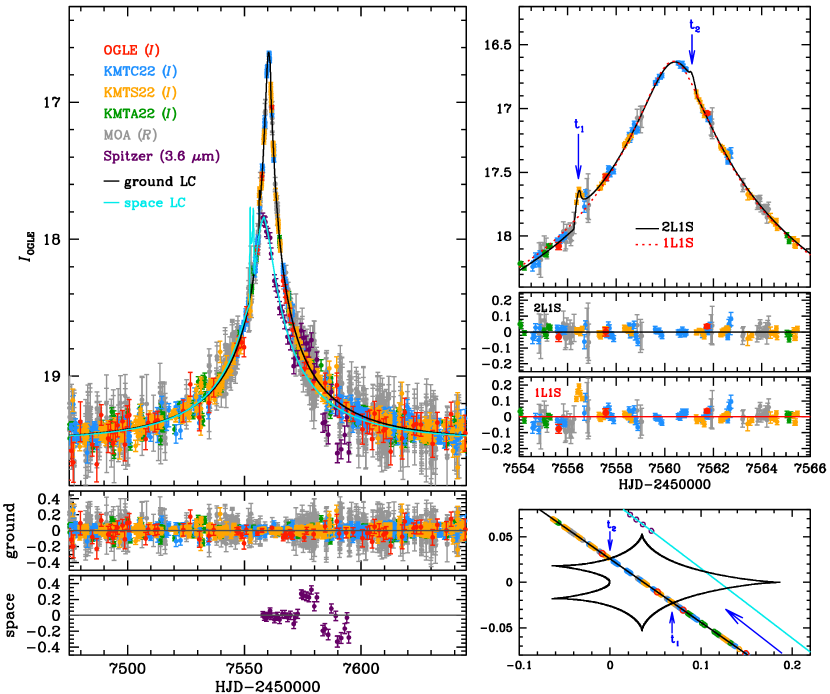
Figure 1: Light curve with the best-fit model (see Table 2). The left panels show the full view of the light curve from both the ground and Spitzer. The upper-right panels show just the ground-based data for the the anomaly part of the light curve (caustic crossings at $t_{1}$ and $t_{2}$), which is induced by the planetary system. For comparison, we present the 1L1S model light curve (dashed red line) with residuals. The lower-right panel presents the caustic geometry of the event.

2 Observations

The microlensing event occurred on a background star (i.e., source) located at $(\alpha,\delta)=(17^{h}56^{m}01^{s}.03,\,-32^{\circ}42{{}^{\prime}}48{{}^{\prime\prime}}.5)$ in equatorial coordinates, which corresponds to $(\ell,b)=(-2^{\circ}.108,\,-3^{\circ}.848)$ in Galactic coordinates. This event was first announced by the Early Warning System (EWS; Udalski et al., 1994; Udalski, 2003) of the Optical Gravitational Lensing Experiment survey (OGLE-IV; Udalski et al., 2015) on 2016 June 11. Thus, this event is designated OGLE-2016-BLG-1093. The event was observed using the $1.3\,m$ Warsaw telescope ($1.4\,{\rm deg}^{2}$ science camera) located at Las Campanas Observatory in Chile.

Two other microlensing surveys independently discovered this event. The Microlensing Observations in Astrophysics (MOA; Bond et al., 2001; Sumi et al., 2003) detected this event on June $24$, $2016$, using the $1.8\,m$ telescope located at the University of Canterbury Mount John Observatory in New Zealand. The Korea Microlensing Telescope Network (KMTNet; Kim et al., 2016) also detected this event using a telescope network consisting of three identical $1.6\,m$ telescopes ($4\,{\rm deg}^{2}$ science cameras) located at the Cerro Tololo Inter-American Observatory in Chile (KMTC), the South African Astronomical Observatory in South Africa (KMTS), and the Siding Spring Observatory in Australia (KMTA). As a result, the light curve of OGLE-2016-BLG-1093 is well covered by five ground-based observatories (see Figure 1).

In addition, this event was chosen as a target of the Spitzer Microlensing Campaign (see Yee et al. 2015 for the details of target selection criteria) and observed using the Spitzer Space Telescope with the $3.6\,{\mu m}$ channel of the IRAC camera. The event was initially selected as a “potentially good” target (i.e., as a “subjective, secret” event) on 2016 June 12 so that observations would be taken during the first week of the Spitzer campaign, i.e., starting 2016 June 18. We announced the event as a “subjective, immediate” event on 2016 June 18 at UT 16:34 (HJD${}^{\prime}=7558.19$), just after the start of the Spitzer observations. We discuss the implications of the selection in Section 7.

Table 1: Best-fit parameters of ground-based models

	1L1S	2L1S			1L2S
Parameter		STD	APRX ($u_{0}<0$)	APRX ($u_{0}>0$)	Parameter
$\chi^{2}_{\rm ground}/{\rm N_{data}}$	$11151.00/10692$	$10688.11/10692$	$10684.919/10692$	$10684.597/10692$	$\chi^{2}_{\rm ground}/{\rm N_{data}}$	$10879.919/10692$
$t_{0}$ [${\rm HJD^{\prime}}$]	$7560.354\pm 0.006$	$7560.317\pm 0.007$	$7560.316\pm 0.007$	$7560.315\pm 0.007$	$t_{0,{S_{1}}}$ $[{\rm HJD^{\prime}}]$	$7560.378\pm 0.006$
$u_{0}$	$0.022\pm 0.001$	$0.021\pm 0.001$	$-0.021\pm 0.001$	$0.021\pm 0.001$	$t_{0,{S_{2}}}$ $[{\rm HJD^{\prime}}]$	$7556.494\pm 0.012$
$t_{\rm E}$ [days]	$54.563\pm 1.164$	$55.395\pm 1.214$	$56.222\pm 1.185$	$56.832\pm 1.312$	$u_{0,{S_{1}}}$	$0.021\pm 0.001$
$s$	$\cdots$	$1.018\pm 0.001$	$1.017\pm 0.001$	$1.017\pm 0.001$	$u_{0,{S_{2}}}$ ($\times 10^{-3}$)	$0.039\pm 0.376$
$q$ ($\times 10^{-3}$)	$\cdots$	$1.536\pm 0.104$	$1.463\pm 0.104$	$1.432\pm 0.109$	$t_{\rm E}$ [days]	$56.815\pm 1.279$
$\alpha$ [rad]	$\cdots$	$2.528\pm 0.026$	$-2.537\pm 0.027$	$2.543\pm 0.027$	$q_{\rm flux}$	$0.003\pm 0.001$
$\rho_{\ast}$ ($\times 10^{-3}$)	$\cdots$	$2.123\pm 0.305$	$2.170\pm 0.293$	$1.883\pm 0.297$	$\rho_{\ast,{S_{1}}}$	$\cdots$
$\pi_{{\rm E},N}$	$\cdots$	$\cdots$	$-0.104\pm 0.102$	$-0.131\pm 0.097$	$\rho_{\ast,{S_{1}}}$ ($\times 10^{-3}$)	$0.921\pm 0.257$
$\pi_{{\rm E},E}$	$\cdots$	$\cdots$	$0.256\pm 0.147$	$0.271\pm 0.149$	$\cdots$	$\cdots$

Note. — ${\rm HJD^{\prime}=HJD-2450000.0}$. For the 1L2S model, the angular radius of the first source ($\rho_{\ast,{S_{1}}}$) is not measured.

3 Ground-based Light Curve Analysis

The light curve of OGLE-2016-BLG-1093 is shown in Figure 1. The event increases in brightness by $\sim 3$ magnitudes suggesting a possible high-magnification event. There is a small perturbation at $t_{\rm pl}=7556.5$. The best-fit point-source/point-lens (1L1S) model has $t_{0}=7560.3$, $t_{\rm E}=55$ days, $u_{0}=0.022$, where $t_{0}$ is the time at the peak of the light curve, $t_{\rm E}$ is the timescale that the source travels the angular Einstein ring radius ($\theta_{\rm E}$), and $u_{0}$ is the separation in units of $\theta_{\rm E}$ at $t_{0}$.

To find the best-fit solution of the binary-lens and single-finite-source (2L1S) model to describe the observed light curve, we first conduct a grid search over the parameters $s$ and $q$. Here, $s$ is the projected separation between binary components, and $q\equiv M_{\rm pl}/M_{\rm h}$ is the mass ratio of binary components, where $M_{\rm pl}$ is the mass of a planet and $M_{\rm h}$ is the mass of a host star. The parameters $s$ and $q$ are related to the caustic morphology. Thus, we set them as grid parameters. For five other parameters of the static 2L1S model (STD), we minimize $\chi^{2}$ using the Markov Chain Monte Carlo algorithm (Dunkley et al., 2005). These five parameters are $t_{0}$, $u_{0}$, $t_{\rm E}$, $\alpha$, and $\rho_{\ast}$. The set of $[t_{0},u_{0},t_{\rm E}]$ are the same as in the 1L1S case, $\alpha$ is the angle of the source trajectory with respect to the binary axis, while $\rho_{\ast}$ is the angular source radius ($\theta_{\ast}$) in units of $\theta_{\rm E}$.

We set a wide range for the $q$ parameter, $\log(q)\in[-5.5,1.0]$. For the $s$ parameter, the grid range is $\log_{10}(s)\in[-1.0,1.0]$. Once we find local minima from the grid search, we use a finer grid to search for localized minima. For competitive solutions found from the grid search, we refine models by allowing all parameters to vary. The best-fit solution has $s\sim 1$ and $q\sim 1.5\times 10^{-3}$. The detailed parameters of this model are presented as the 2L1S STD solution in Table 1.

We find that the light curve of OGLE-2016-BLG-1093 is qualitatively similar to that of KMT-2019-BLG-0842Lb (Jung et al., 2020) or OGLE-2019-BLG-0960Lb (Yee et al., 2021), both of which have much smaller mass ratios ($q<10^{-4}$) than our best-fit solution. Following the formalism of Gaudi & Gould (1997), we estimate the properties of such a solution. Because the planetary perturbation occurs at $u_{\rm pl}\equiv\sqrt{u_{0}^{2}+\tau_{\rm pl}^{2}}=0.074$, where $\tau_{\rm pl}\equiv(t_{\rm pl}-t_{0})/t_{\rm E}=0.069$, this line of reasoning would imply $s=\left[\sqrt{\left(u_{\rm pl}^{2}+4\right)}+u_{\rm pl}\right]/2=1.04$ and $\alpha=\tan^{-1}(u_{0}/\tau_{\rm pl})=162^{\circ}$ (2.83 radians). Such a trajectory would be very similar to those of KMT-2019-BLG-0842Lb and OGLE-2019-BLG-0960Lb. Hence, one might expect that OGLE-2016-BLG-1093 may also contain a planet with a very small mass ratio. Thus, we explicitly search for small mass-ratio solutions similar to KMT-2019-BLG-0842Lb and OGLE-2019-BLG-0960Lb, but find that those solutions are disfavored by $\Delta\chi^{2}\sim 180$ compared to the $(s,q)\sim(1,1.5\times 10^{-3})$ solution.

3.1 Annual Microlens Parallax (APRX)

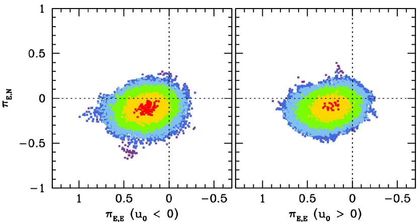
Figure 2: The ($\mbox{$\pi_{{\rm E},E}$},\,\mbox{$\pi_{{\rm E},N}$}$) contours of the APRX models. Each color indicates $\Delta\chi^{2}_{\rm(chain-best)}\leq n^{2}$, where $n=1$ (red), $2$ (yellow), $3$ (green), $4$ (light blue), $5$ (blue), and $6$ (purple), respectively.

The ground-based light curve analysis shows that the timescale of this event is $\sim 55.4$ days. This is long enough ($t_{\rm E}>15$ days) to check the effect caused by the annual microlens parallax (APRX; Gould, 1992) on the light curve. Thus, we try to check the APRX effect by introducing the microlens-parallax parameters: ($\pi_{{\rm E},N}$, $\pi_{{\rm E},E}$), which indicate the north and east directions of the microlens-parallax vector ($\mbox{\boldmath$\pi$}_{\rm E}$), respectively.

In Table 1, we present the best-fit parameters of APRX models. From the APRX modeling, we find $\chi^{2}$ improvements of $\Delta\chi^{2}=3.2$ and $\Delta\chi^{2}=3.5$ for ($u_{0}<0$) and ($u_{0}>0$) cases, respectively. These improvements are too minor to claim that the APRX measurements can be used to determine the lens properties.

However, we find that the APRX contours do not represent a complete non-detection of the APRX effect. The contours are well converged as shown in Figure 2, which gives strong upper limits on the parallax.

3.2 Lens-orbital Effect

Because the orbital motion of the binary components can affect the APRX (Batista et al., 2011), we also check the lens-orbital (OBT) only model by introducing the lens-orbital parameters: $(ds/dt,\,d\alpha/dt)$ where $ds/dt$ is the variation of the binary separation as a function of time and $d\alpha/dt$ is the variation of the source trajectory angle as a function of time.

We find a negligible $\chi^{2}$ improvement (i.e., $\Delta\chi^{2}_{\rm(STD-OBT)}=1.67$) when the lens-orbital effect is considered. Also, we find that this very small improvement comes from outside the region of the caustic-crossing. In general, the lens-orbital effect is most sensitive to the caustic-crossing parts of the light curve (that are mostly covered by KMTC and KMTS). Thus, we can conclude that there is no significant lens-orbital effect for this event.

3.3 2L1S/1L2S Degeneracy

As Gaudi (1998) pointed out, the single-lens/binary-source (1L2S) interpretation can mimic planetary anomalies. Also, Shin et al. (2019) shows that this 2L1S/1L2S degeneracy can appear in wider ranges of cases, especially, the degeneracy appears in cases having non-optimal observational coverage.

For this event, there is a gap in the observational coverage of the second bump. Thus, we check the 2L1S/1L2S degeneracy. For the 1L2S model, we adopt parameters described in Shin et al. (2019) (A-type, see Appendix of the reference) shown in Table 1. We find that the $\chi^{2}$ difference between the 1L2S and 2L1S models is $\sim 192$, which is enough to resolve the degeneracy. In particular, the 1L2S cannot properly describe the caustic-crossing feature of the first bump. Thus, we conclude that this event does not suffer from the 2L1S/1L2S degeneracy.

4 Spitzer Parallax

4.1 Joint Spitzer$~{}+$ Ground

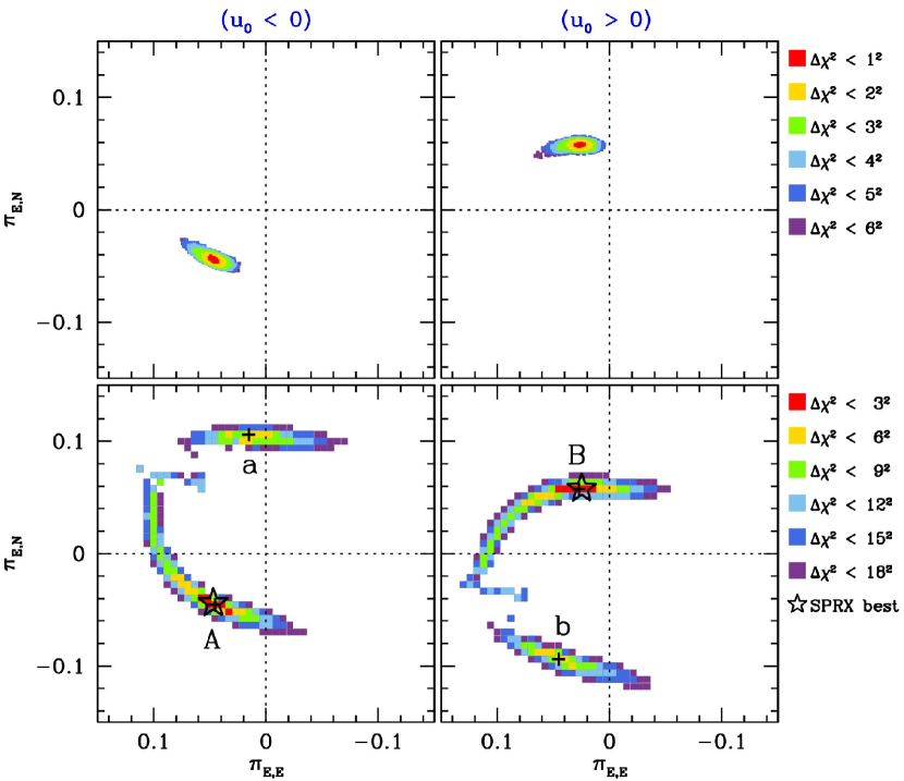
Figure 3: The ($\pi_{{\rm E},E}$, $\pi_{{\rm E},N}$) contours of SPRX models. Top panels show SPRX contours of Joint Spitzer$~{}+$ Ground cases. Bottom panels show SPRX contours of Spitzer-“only” cases. Right and left panels present ($u_{0}<0$) and ($u_{0}>0$) cases, respectively. The black stars indicate the best-fit ($\pi_{{\rm E},E}$, $\pi_{{\rm E},N}$) values of Joint Spitzer$+$ Ground cases. The labeled black $+$’s indicate the ($\pi_{{\rm E},N}$, $\pi_{{\rm E},N}$) locations of the four minima shown in Figure 4

To measure the microlens parallax effect using Spitzer data, we jointly fit the Spitzer and ground-based light curves. This fit is constrained by a color-color relation constructed from nearby stars:

$$(I-L)_{\rm pyDIA}=-5.505\pm 0.025.$$ (1)

We note that the color constraint for modeling is $(I-L)_{\rm pySIS}=2.218\pm 0.025$ (allowed $2\sigma$ ranges). The value of this color constraint is different from the value shown in Equation 1. Because the Spitzer zero point of the color constraint shown in Equation 1 is $25$ magnitude. However, for our modeling scheme, we use an $18$ magnitude as the zero point. Thus, we convert the magnitude system from $25$th to $18$th by adding $7$ magnitudes. In addition, we use the “pySIS” photometry of KMTC for modeling to use the best quality of photometry. While, we use the “pyDIA” photometry for the source color estimation (the “pyDIA” photometry is optimized to obtain $V$-band light curve and the color-magnitude diagrams). These two datasets have different zero points. For this event, the relation between them is $I_{\rm pySIS}-I_{\rm pyDIA}=0.723\pm 0.002$. Thus, the final color constraint for the modeling is that $(I-L)_{\rm pySIS}=(I-L)_{\rm pyDIA}+7+0.723=2.218\pm 0.025$. We apply the color constraint on the models using an additional $\chi^{2}$ (i.e., $\chi^{2}_{\rm penalty}$) that is weighted by the different amount of the source color. The details of $\chi^{2}_{\rm penalty}$ are described in Shin et al. (2017).

The top panels of Figure 3 show that the resulting constraints on the parallax are very tight for the both $(u_{0}<0)$ and $(u_{0}>0)$ solutions. These panels show two well-constrained minima at $\mbox{\boldmath$\pi$}_{\rm E}(N,E)=(-0.044,0.047)$ and $(0.058,0.025)$ for the $(u_{0}<0)$ and $(u_{0}>0)$ solutions, respectively. This is in contrast to the “usual” situation for point lens events, which typically show a four-fold degeneracy (Refsdal, 1966; Gould, 1994) or an arc (often seen for partial light-curves like this one; Gould, 2019). We revisit this degeneracy in the next section. These minima imply parallax values of $\pi_{\rm E}=0.064$ and $0.063$, respectively. They are also consistent with the broad constraints on the parallax from the annual parallax effect (see Figure 2). The full fits are given in Table 2.

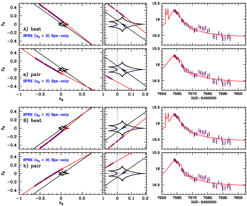
Figure 4: Four solutions from Spitzer-“only” fitting. Left panels show the trajectories of the source as seen from the ground (black line with arrow) and Spitzer (red line with arrows) over the full span of the observations from Spitzer (epochs of observations shown as purple circles). The caustics are shown as a black, closed curve. Center panels show a zoom of the caustic region. Right panels show the Spitzer light curve (purple points) with the best-fit model light curve (red line) for each solution. The “a” and “b” solutions are disfavored relative to the “A” and “B” solutions; lettering corresponds to the minima indicated in Figure 3.

Table 2: Best-fit parameters of SPRX Tests with the ($I-L$) color constraint

	SPRX		Cheap-SPRX
Parameter	($u_{0}<0$)	($u_{0}>0$)	($u_{0}<0$)	($u_{0}>0$)
$\chi^{2}_{\rm Total}$	$10735.013$	$10737.220$	$10687.513$	$10686.936$
$\chi^{2}_{\rm ground}/{\rm N_{data}}$	$10686.57/10692$	$10689.34/10692$	$10686.55/10692$	$10686.07/10692$
$\chi^{2}_{\rm Spitzer}/{\rm N_{data}}$	$48.28/36$	$47.70/36$	$0.84/4$	$0.84/4$
$\chi^{2}_{\rm penalty}$	$0.164$	$0.125$	$0.121$	$0.030$
$t_{0}$ [${\rm HJD^{\prime}}$]	$7560.318\pm 0.007$	$7560.319\pm 0.007$	$7560.315\pm 0.007$	$7560.318\pm 0.007$
$u_{0}$	$-0.021\pm 0.001$	$0.021\pm 0.001$	$-0.021\pm 0.001$	$0.021\pm 0.001$
$t_{\rm E}$ [days]	$56.355\pm 1.168$	$56.311\pm 1.242$	$55.401\pm 1.241$	$56.370\pm 1.241$
$s$	$1.017\pm 0.001$	$1.017\pm 0.001$	$1.018\pm 0.001$	$1.018\pm 0.001$
$q$ ($\times 10^{-3}$)	$1.473\pm 0.099$	$1.470\pm 0.102$	$1.523\pm 0.105$	$1.469\pm 0.104$
$\alpha$ [rad]	$-2.532\pm 0.026$	$2.535\pm 0.025$	$-2.532\pm 0.026$	$2.531\pm 0.026$
$\rho_{\ast}$ ($\times 10^{-3}$)	$2.142\pm 0.303$	$2.103\pm 0.309$	$2.216\pm 0.312$	$2.185\pm 0.312$
$\pi_{{\rm E},N}$	$-0.044\pm 0.003$	$0.058\pm 0.002$	$\cdots$	$\cdots$
$\pi_{{\rm E},E}$	$0.047\pm 0.006$	$0.025\pm 0.006$	$\cdots$	$\cdots$
$|\pi_{{\rm E}}|$	$0.064\pm 0.003$	$0.063\pm 0.003$	$0.066_{-0.010}^{+0.013}$	$0.088_{-0.027}^{+0.007}$
$f_{\rm S,KMTC\,{\it(I)}}$	$0.044\pm 0.001$	$0.044\pm 0.001$	$0.045\pm 0.001$	$0.044\pm 0.001$
$f_{\rm S,Spitzer,{\it(L)}}$	$0.341\pm 0.011$	$0.341\pm 0.011$	$0.341\pm 0.011$	$0.339\pm 0.011$
$(I-L)_{\rm pySIS}$	$2.223\pm 0.043$	$2.223\pm 0.043$	$2.209\pm 0.043$	$2.223\pm 0.043$

4.2 Spitzer-“only”

As a check, we also conduct the Spitzer-“only” test for the full Spitzer dataset. We conduct this Spitzer-“only” analysis following the formalism laid out in Gould et al. (2020) but using a full planet model as in Zang et al. (2020). Specifically, we fix the seven parameters of the model ($t_{0}$, $u_{0}$, $t_{E}$, $\rho$, $\alpha$, $s$, $q$) to their ground-based values, vary $\pi_{E,N}$ and $\pi_{E,E}$ on a grid, and fit only the Spitzer data with the color-constraint applied. The resulting parallax constraints shown in the bottom panels of Figure 3 are more extended arcs compared to the constraints from the full, joint fit. In fact, they show four local minima as might be expected from the four-fold degeneracy discussed above. Nevertheless, the four-fold degeneracy is broken because the caustic structure induces additional structure to the light curve (see Figure 4), and the Spitzer-“only” fits ultimately recover the same global minimum in each case ($u_{0}>0$ and $u_{0}<0$). Then, comparing the top and bottom panels in Figure 3 shows that the joint fitting further suppresses these alternate minima leaving a two-fold degeneracy rather than a four-fold degeneracy.

5 Tests of the Spitzer Parallax

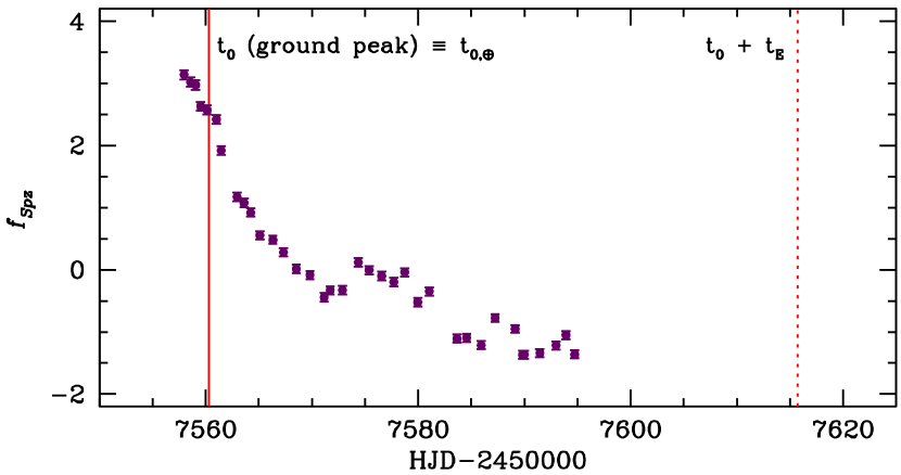
Figure 5: Spitzer light curve in instrumental flux units. The solid vertical line indicates the peak of the light curve as observed from Earth ($t_{0}\equiv t_{0,\oplus}$) and the dotted vertical line is $+t_{\rm E}$ away.

Koshimoto & Bennett (2020) have suggested that systematics in the Spitzer light curve may bias the resulting parallax measurements. Such systematics have been seen at the level of 1–2 instrumental flux units (Gould et al., 2020; Hirao et al., 2020; Zang et al., 2020), and so are most likely to play a significant role in events with small changes in flux as measured by Spitzer. Figure 5 shows the Spitzer light curve of OGLE-2016-BLG-1093 in instrumental flux units and illustrates that it is in this regime. However, because OGLE-2016-BLG-1093 is in the high-magnification regime, this permits several tests that can be used to verify the parallax signal, which we describe below.

5.1 Heuristic Analysis

First, overall, the Spitzer light curve appears to decline during the Spitzer observation window, suggesting that the event peaked earlier as seen from the ground. Because Spitzer was separated from Earth by $D_{\perp}=1.021$ au (as projected on the sky), this suggests $\pi_{\rm E}>\Delta\tau\,({\rm AU}/D_{\perp})$ where $\tau=(t_{0,\oplus}-t_{\rm start,Spz})/t_{\rm E}=0.043$, so $\pi_{\rm E}>0.042$, which is consistent with the values derived from the full-fit.

Second, the characteristics of OGLE-2016-BLG-1093 are similar to the criteria set out by Gould & Yee (2012) for “cheap-space parallaxes”. Specifically, the event is in the high-magnification regime ($A_{\rm peak}\sim 50$), the Spitzer observations start before the ground-based peak ($t_{\rm start,Spz}=7558.0<t_{0,\oplus}=7560.3$), and, as we show below, was observed by Spitzer close to baseline. The basic logic is that if Spitzer observes at the peak as seen from the ground, then $u_{\oplus}\sim 0$ and

$$\pi_{\rm E}\sim\frac{{\rm AU}}{D_{\perp}}u_{\rm Spz}.$$ (2)

In this case, we observe $\Delta f_{\rm Spz}\sim 4$ flux units (between $t_{0,\oplus}$ and $t_{\rm last,Spz}$), and we can estimate $f_{\rm source,Spz}$ from the color-color relation in Equation 1. Given $I_{\rm source}=20.9$, this implies $f_{\rm source,Spz}=0.274$. The last Spitzer observation is taken at HJD${}^{\prime}=7589.1$ when the event is magnified by $A_{\oplus}=2.1$ as seen from Earth. Because we know the event peaked earlier from Spitzer, we know that $A_{\rm last,Spz}<2.1$. Then,

$$\begin{split}\Delta f_{\rm Spz}&=f_{\rm Spz}(t_{0,\oplus})-f_{\rm Spz}(7589.1)\\ &=f_{\rm source,Spz}[A_{\rm Spz}(t_{0,\oplus})-A_{\rm last,Spz}],\end{split}$$ (3)

Hence, $15.6<A_{\rm Spz}(t_{0,\oplus})<16.7$. This yields $0.060<u_{\rm Spz}(t_{0,\oplus})<0.064$ and an estimate of the parallax: $0.059<\pi_{\rm E}<0.063$ (for $D_{\perp}=1.021$ au), although the parallax could be somewhat larger for $u_{\oplus}>0$.

An additional caveat is that the “cheap-space parallaxes” formalism was developed for point lenses, whereas OGLE-2016-BLG-1093 contains a large resonant caustic structure. This caustic structure has the potential to cause this formalism to break down. At the same time, we can already see that the measured values of the parallax are in good agreement with this simplified heuristic analysis.

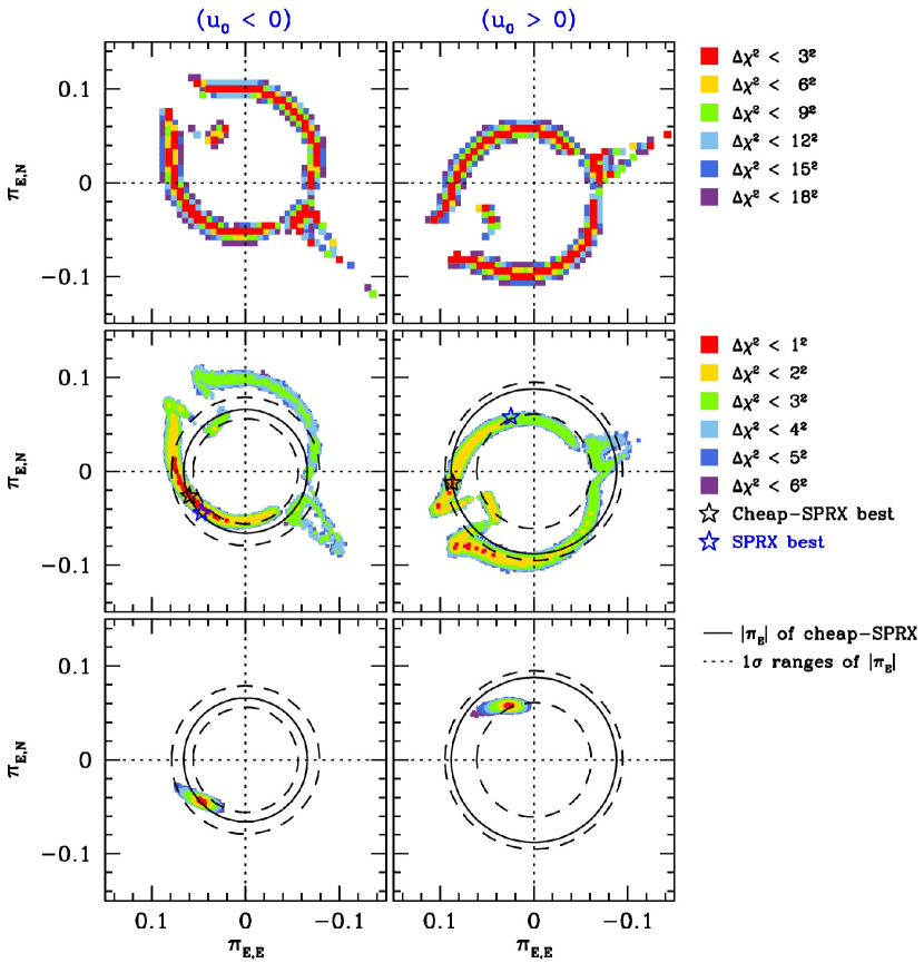
Figure 6: The ($\pi_{{\rm E},E}$, $\pi_{{\rm E},N}$) contours of cheap–SPRX models with SPRX contours for comparison. Top panels show cheap–SPRX contours of Spitzer–“only” cases. Middle panels show cheap–SPRX contours of Joint Spitzer$~{}+$ Ground cases. The bottom panels show the SPRX contours for comparison. The right and left panels present the ($u_{0}<0$) and ($u_{0}>0$)cases, respectively. The circles indicate $|\pi_{{\rm E}}|$ values (solid lines) measured from the cheap–SPRX with their $1\sigma$ errors (dashed lines). The blue and black star marks indicate the best-fit values of SPRX and cheap–SPRX models, respectively.

5.2 Cheap-Space Parallax Limit

To further explore the application of “cheap-space parallaxes” to this event, we next fit a subset of the Spitzer data, as might be obtained by such an observational program. Specifically, we restrict the fitting to the Spitzer observation taken closest to $t_{0,\oplus}$ and the last three Spitzer observations (technically, only the last observation is needed, but the observed scatter in the light curve suggests that, in this case, a single observation may not accurately reflect the mean magnification). Under the “cheap-space parallaxes” formalism, for a points lens with $u_{0}=0$, we would expect this test to produce an annulus on the $\mbox{\boldmath$\pi$}_{\rm E}$ plane centered at the origin (e.g., Shin et al., 2018).

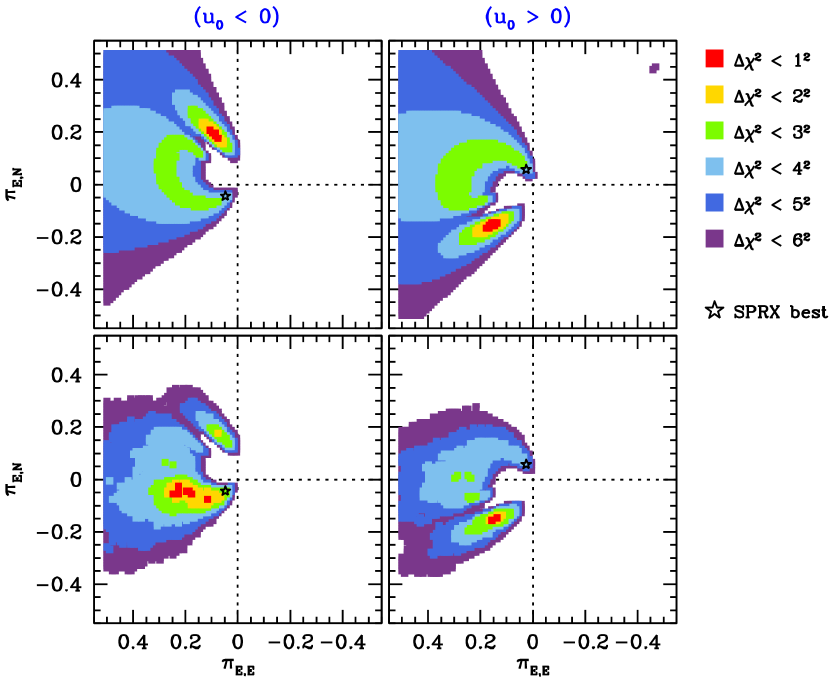
Figure 7: Constraints on the microlens parallax vector without including the color constraint. The top panels show Spitzer-“only” cases. The bottom panels show Spitzer$+$ Ground cases. The star mark indicates the best-fit parallax with including the color constraint. These differ significantly from the constraints in Figure 3 because the correlated noise in the Spitzer light curve can be fit by the planetary model if an arbitrary source flux is allowed.

5.2.1 Spitzer-“only” Cheap-Space Parallaxes

For the first test, we conduct Spitzer-“only” fitting with this restricted dataset. The full contours are shown in the top panels of Figure 6. They show that, for this event with its large resonant caustic, the contours are still similar to a ring shape. That ring is displaced from the origin by $\sim u_{0,\oplus}$, as would be expected for the 1L1S case with $|u_{0,\oplus}|>0$. The uncertainty in $\pi_{\rm E}$ due to $|u_{0,\oplus}|>0$ is comparable to the uncertainty due to 2L1S departures from the ring-shape. This indicates that the “cheap-space parallaxes” formalism still applies in 2L1S cases with $q\ll 1$ (i.e., the magnification map is still dominated by the effect of the primary lens).

Finally, from this fit, we derive $0.06<\mbox{$|\pi_{{\rm E}}|$}<0.10$, which much stronger than the constraint from APRX alone and constrains the lens to be in the bulge (when combined with $\theta_{\rm E}$, see Section 6).

5.2.2 Spitzer $+$ Ground Cheap-Space Parallaxes

We also conduct a joint fit to the ground-based data and the “cheap-space parallax” subset of the Spitzer data (and including the color-constraint). The results of the joint fit are shown in the middle panels of Figure 6 and the parameters are given in Table 2. These contours show the influence of the APRX constraint from the ground-based data, which weakly prefer parallaxes in the middle-left panel. Hence, in the “cheap-space parallax” limit, even weak constraints or upper limits from APRX can be meaningful.

5.3 Test of Spitzer Systematics

5.3.1 Role of the Color-constraint

Because the overall change in the Spitzer flux is small relative to the magnitude of the systematics, the color-constraint plays a very important role in this event. When we fit the Spitzer data without including the color-constraint, we find a completely different solution for the parallax. Figure 7 shows the contours for the Spitzer-“only” case without the color-constraint (the joint fit is similar because of the weakness of the APRX). For the best-fit solution, $f_{\rm S,Spz}\sim 0.9$, which a factor of $\sim 3$ larger than the value expected from the color-constraint (Section 5.1). Close inspection of the Spitzer light curve in Figure 5 shows an apparent “dip” in the light curve between HJD${}^{\prime}\sim 7561$ and HJD${}^{\prime}\sim 7574$ at the level of $\sim 1$ flux unit compared to a smooth decline. Thus, in the absence of the color-constraint, this dip can be fit by the “trough” induced by the $s<1.02$ planet. This confirms that correlated noise can exist in the Spitzer light curves at the level of $\sim 1$ flux unit.

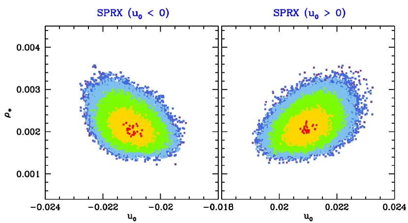
Figure 8: The contours of the $\rho_{\ast}$ parameter. The color scheme is identical to Figure 2.

5.3.2 Potential Impact of Systematics

Systematics at the level of $\sim 1$ flux unit have been seen in several events (e.g., Poleski et al., 2016; Dang et al., 2020; Gould et al., 2020; Hirao et al., 2020) and are confirmed in this case. The potential impact of systematics will be most pronounced in events for which the overall flux change is small (e.g., for $\Delta f_{\rm Spz}\lesssim 10$ flux units). For example, such an impact was seen in KB180029 (Gould et al., 2020), for which the baseline flux differed by $\sim 1$ flux unit between seasons.

Because the overall flux change in OGLE-2016-BLG-1093 is only $\Delta f_{\rm Spz}\sim 4$ flux units, we briefly consider how such systematics might affect the parallax. We have already shown that the “cheap-space parallaxes” formalism is a reasonable approximation in this case and that our simple estimate of the parallax from Section 5.1 is reasonably accurate. If systematics affect either (or both) the peak or the baseline of the Spitzer light curve for OGLE-2016-BLG-1093, then the true change in flux might be as low as 3 flux units or as high as 5 flux units. Taking into account this range of fluxes (and the uncertainty in $A_{\rm last}$), the parallax would still be confined to the range $\pi_{\rm E}=[0.05,0.08]$, yielding a factor of $\sim 1.3$ uncertainty in the lens mass and a $\sim 0.25$ kpc uncertainty in the distance. Hence, the lens is still constrained to be a low-mass dwarf in the bulge.

6 Source Color and Lens Properties

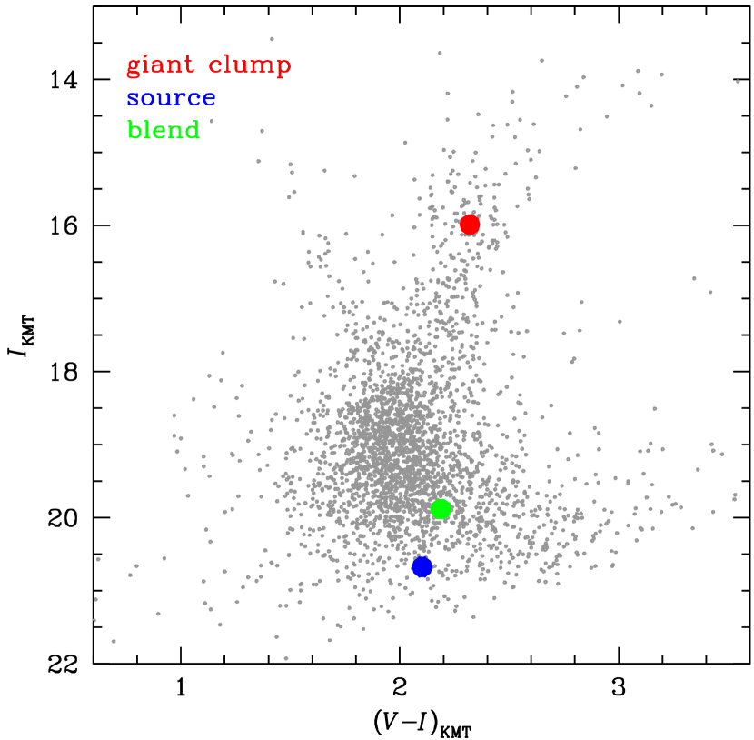
Figure 9: Color-magnitude diagrams of the KMTNet.

6.1 Finite-source Effect

In addition to measuring $\pi_{\rm E}$, one must also determine the angular Einstein ring radius ($\theta_{\rm E}$), in order to derive the lens properties such as mass of the lens system ($M_{\rm L}$ and the distance to the lens system ($D_{\rm L}$):

$$M_{\rm L}=\frac{\theta_{\rm E}}{\kappa\pi_{\rm E}},~{}~{}D_{\rm L}=\frac{\rm au}{\pi_{\rm E}\theta_{\rm E}+\pi_{\rm S}},$$ (4)

where $\kappa=8.144\,{\rm mas}\,M_{\odot}^{-1}$, $\pi_{\rm S}\equiv{\rm au}/D_{\rm S}$ is the parallax of the source, and $D_{\rm S}$ is a distance to the source.

The $\theta_{\rm E}$ can be determined using the finite-source effect: $\rho_{\ast}\equiv\theta_{\ast}/\theta_{\rm E}$ where $\theta_{\ast}$ is the angular source radius, which is an observable that can be routinely measured (see Section 6.2). For this event, there are caustic-crossing features that are well-covered by KMTS and KMTC. Thus, it is possible to measure $\rho_{\ast}$ from the finite-source effect. In Figure 8, we present the contours of $\rho_{\ast}$. The contours show that the $\rho_{\ast}$ values are securely measured.

Table 3: Lens properties determined using SPRX and cheap–SPRX

	SPRX		Cheap-SPRX
Properties	($u_{0}<0$)	($u_{0}>0$)	($u_{0}<0$)	($u_{0}>0$)
$\theta_{\rm E}$ (mas)	$0.24\pm 0.04$	$0.25\pm 0.04$	$0.23\pm 0.04$	$0.24\pm 0.04$
$M_{\rm host}$ ($M_{\odot}$)	$0.46\pm 0.08$	$0.48\pm 0.09$	$[0.31,0.60]$	$[0.25,0.56]$
$M_{\rm planet}$ ($M_{\rm Jup}$)	$0.71\pm 0.12$	$0.74\pm 0.13$	$[0.49,0.96]$	$[0.39,0.86]$
$D_{\rm S}$ (kpc)	$9.40\pm 0.87$	$9.39\pm 1.21$	$9.16\pm 1.08$	$9.20\pm 1.09$
$D_{\rm L}$ (kpc)	$8.12\pm 0.69$	$8.06\pm 0.91$	$7.93\pm 0.84$	$7.79\pm 0.82$
$D_{\rm LS}$ (kpc)	$1.28\pm 0.27$	$1.33\pm 0.37$	$1.23\pm 0.36$	$1.41\pm 0.43$
$a_{\perp}$ (au)	$2.13\pm 0.33$	$2.23\pm 0.43$	$2.01\pm 0.34$	$2.00\pm 0.34$

6.2 Angular Source Radius

The angular source radius can be measured using the conventional method (Yoo et al., 2004). The method requires multi-band observations. The KMTNet survey regularly observes $V$-band data. In $2016$, KMTC made one $V$-band observation for every $10$ $I$-band observations, while KMTS made $V$-band observations at half this rate. We use the KMTC observations to determine the color. Using the multi-band observations, we construct the KMTNet color-magnitude diagrams (CMD) shown in Figure 9. Then, we measure the reddened and de-reddened colors of the source using Yoo et al.’s method and the intrinsic color and magnitude of the red giant clump adopted from Bensby et al. (2011) and Nataf et al. (2013):

$$(V-I)=2.102\pm 0.013,$$ (5)

$$(V-I)_{0}=0.842\pm 0.052.$$ (6)

We estimate the angular source radius using the color conversion of Bessell & Brett (1988) and the color/surface-brightness relation of Kervella et al. (2004):

$$\theta_{\ast}=0.52\pm 0.03\,\mu{\rm as}$$ (7)

Then, by combining the $\rho_{\ast}$ measurements, we determine the angular Einstein ring radius of each solution shown in Table 3.

6.3 Lens properties

In Table 3, we present lens properties determined using measurements of $|\pi_{{\rm E}}|$ and $\theta_{\rm E}$ (see Equation 4). The binary lens system is revealed as a planetary system consisting of a sub-Jupiter-mass planet ($M_{\rm pl}\sim 0.7\,M_{\rm Jup}$) orbiting an M-dwarf host star ($M_{\rm h}\sim 0.5\,M_{\odot}$) with a projected separation of $\sim 2$ au.

Because the source distance is not precisely known, $\pi_{\rm rel}$ (and therefore $D_{\rm LS}\equiv D_{\rm S}-D_{\rm L}\simeq\left(\pi_{\rm rel}/{\rm au}\right)D_{\rm clump}^{2}$) is much better constrained than $D_{\rm L}$. Here, we adopt $D_{\rm clump}=8.54$ kpc from Nataf et al. (2013). We find

$$D_{\rm LS}\simeq\frac{\pi_{\rm rel}}{\rm au}D_{\rm clump}^{2}=1.1\pm 0.2\,{\rm kpc}$$ (8)

Because, the source is almost certainly in the bulge, this small value of $D_{\rm LS}$ provides strong evidence that the lens is in the bulge as well.

Moreover, we estimate distances to lens ($D_{\rm L}$) and source ($D_{\rm S}$) using the Bayesian analysis with constraints of $t_{\rm E}$, $\theta_{\rm E}$, and $\mbox{\boldmath$\pi$}_{\rm E}$. The Bayesian formalism is adopted from Shin et al. (2021) with the mass function of Chabrier (2003). The Bayesian results indicate that the lens is located at the bulge ($D_{\rm L}\sim 8.1$ kpc). This result directly supports the $D_{\rm LS}$ argument, which shows the planet is located in the bulge. We present the distances of each case in Table 3.

7 Membership in the Spitzer sample

According to the protocols of Yee et al. (2015), because the first Spitzer observation (at HJD${}^{\prime}=7557.96$) was taken before the event was announced as a Spitzer target, this point must be excluded from the evaluation of the Spitzer parallax for the purposes of evaluating whether or not the event is part of the statistical Spitzer planet sample. Therefore, we repeat the joint ground+Spitzer fitting but without the first Spitzer observation. We find $\mbox{$|\pi_{{\rm E}}|$}=0.062\pm 0.003$ and $\mbox{$|\pi_{{\rm E}}|$}=0.063\pm 0.003$ for the $(u_{0}<0)$ and $(u_{0}>0)$ solutions, respectively.

In terms of calculating membership in the Spitzer sample, we need to calculate $D_{8.3}$ and its uncertainty (i.e., the lens distance for a source at 8.3 kpc, see Zhu et al. 2017 for details). We find $D_{8.3}=7.3$ kpc and $\sigma_{D_{8.3}}=0.2$ kpc. According to Zhu et al. (2017), events with $\sigma_{D_{8.3}}<1.4$ kpc can be included in the statistical Spitzer sample. Hence, OGLE-2016-BLG-1093 meets this criterion.

Then, we should consider whether or not the planet in OGLE-2016-BLG-1093 can be included in the sample. Yee et al. (2015) have specified that only planets (and planet sensitivity) from after the selection can be included in the statistical analysis. In this case, the event was not selected until HJD${}^{\prime}=7558.19$, which is after the planet perturbation at $\sim 7556.5$. However, the last datum that was available to the Spitzer team when it made its decision was at $7555.63$, i.e., before the anomaly. That is, although at the time of the decision, OGLE had taken one additional observation (at $7557.57$), this was not posted to the OGLE web page until $7558.29$, i.e., after the decision. Moreover, MOA did not issue its alert until $7564.05$, and KMT did not reduce its data until after the season. The anomaly was first recognized by KMTNet member K.-H. Hwang in May 2019. Hence, no information about the planet (or possible planet) was available to the team at the time of the decision and all of the KMT and MOA data can be included in the statistical analysis.

8 Conclusions

Using Spitzer  parallax combined with finite source effects, we find that OGLE-2016-BLG-1093Lb is a sub-Jupiter-mass planet with the mass of $0.59$–$0.87\,M_{\rm Jup}$. This planet lies beyond the snow line ($a_{\perp}\sim 2$ au) of an M-dwarf host with the mass of $0.38$–$0.57\,M_{\odot}$ ($a_{\rm snow}=1.0$–$1.5$ au: Kennedy & Kenyon, 2008). This planet is part of the statistical sample of Spitzer microlensing planets with measured distances. Although the planet perturbation occurred prior to the selection of the event for Spitzer observations, no anomalous data points were available to the Spitzer Team until after it made its selection, and so it meets the criteria of Yee et al. (2015) for inclusion in the sample. Including, OGLE-2016-BLG-1093Lb, the total number of planets in the sample is now eight (two-thirds of the expected number for the program). Moreover, the recent discovery of the planet in OGLE-2019-BLG-1053 (Zang et al., 2021) suggests additional planets remain undiscovered in the Spitzer sample.

Because this is a high magnification event ($A_{\rm max}\sim 50$), we are able to conduct a number of tests of the SPRX measurement. First, we conducted a test by adopting the cheap–SPRX idea from Gould & Yee (2012), in which we use only the Spitzer data taken closest to the ground-based peak of the event and the least magnified points. From this test, we found that the cheap–SPRX measurement is consistent with the full SPRX measurement at the $1\sigma$ level. This test demonstrates that the cheap space-parallax method can be applied to 2-body lenses in addition to point lenses, at least in cases for which the 2-body perturbation is small relative to the overall magnification effect.

We also perform the Spitzer-“only” test from Gould et al. (2020) and investigate systematics in the Spitzer light curve. Because the annual parallax signal is very weak, the Spitzer-“only” test is very similar to the joint Spitzer+ ground fitting for the full dataset; i.e., the parallax measurement is dominated by the SPRX. However, it has some influence on the “cheap–SPRX” fits because relatively little Spitzer data are used. Finally, we confirm that there are systematics in the Spitzer light curve of OGLE-2016-BLG-1093 at the $\sim 1$ flux unit level. In a completely free fit, these systematics may be fit by features in the planetary magnification pattern. However, such models are ruled out once the constraint on the source flux is included.

In addition to OGLE-2016-BLG-1093Lb, there are several other cases of giant planets with distances measured to be in or very near the bulge. Based on measurements of the lens flux resolved from the source, Vandorou et al. (2020) find $m_{p}=2.74\,M_{\rm Jup}$, $D_{L}=6.72$ kpc for MOA-2013-BLG-220Lb, and Bhattacharya et al. (2021) find $m_{p}=1.71\,M_{\rm Jup}$, $D_{L}=6.89$ kpc for MOA-2007-BLG-400Lb. Batista et al. (2014) measured a flux excess for MOA-2011-BLG-293 and inferred $m_{p}=4.8\,M_{\rm Jup}$, $D_{L}=7.72$ kpc assuming this excess is due to the lens. However, Koshimoto et al. (2020) have suggested this excess is due to a source companion rather than lens; nevertheless, they still infer a giant planet in or near the bulge. In addition, the planet in OGLE-2016-BLG-1093 is similar to OGLE-2017-BLG-1140Lb, which is $1.6\,M_{\rm Jup}$ planet orbiting a $0.2\,M_{\odot}$ host with $D_{8.3}=7.4\,$ kpc (see Zhu et al., 2017, for the definition of $D_{8.3}$); although, in that case, the measured proper motions suggested that the lens was a member of the disk population. Regardless, the growing number of detected giant planets at bulge distances would seem to contradict the expectation from Thompson (2013) that giant planets cannot form in the bulge. OGLE-2016-BLG-1093 also suggests a definitive answer will be possible once analysis of the full Spitzer sample is complete.

Acknowledgments. This research has made use of the KMTNet system operated by the Korea Astronomy and Space Science Institute (KASI), and the data were obtained at three host sites of CTIO in Chile, SAAO in South Africa, and SSO in Australia. Work by C.H. was supported by grants of the National Research Foundation of Korea (2017R1A4A1015178 and 2019R1A2C2085965). J.C.Y. acknowledges support from N.S.F Grant No. AST–2108414 and JPL grant 1571564. The MOA project is supported by JSPS KAK–ENHI Grant Number JSPS24253004, JSPS26247023, JSPS23340064, JSPS15H00781, JP16H06287,17H02871 and 19KK0082.

References

- Batista et al. (2011) Batista, V., Gould, A., Dieters, S., et al. 2011, A&A, 529, A102
- Batista et al. (2014) Batista, V., Beaulieu, J.-P., Gould, A., et al. 2014, ApJ, 780, 54
- Bensby et al. (2011) Bensby, T., Adén, D., Meléndez, J., et al. 2011, A&A, 533, A134
- Bessell & Brett (1988) Bessell, M. S. & Brett, J. M. 1988, PASP, 100, 1134
- Bhattacharya et al. (2021) Bhattacharya, A., Bennett, D. P., Beaulieu, J. P., et al. 2021, AJ, 162, 60
- Bond et al. (2001) Bond, I. A., Abe, F., Dodd, R. J., et al. 2001, MNRAS, 327, 868
- Calchi Novati et al. (2015) Calchi Novati, S., Gould, A., Udalski, A., et al. 2015, ApJ, 804, 20
- Calchi Novati et al. (2018) Calchi Novati, S., Skowron, J., Jung, Y. K., et al. 2018, AJ, 155, 261
- Chabrier (2003) Chabrier, G. 2003, PASP, 115, 763
- Dang et al. (2020) Dang, L., Calchi Novati, S., Carey, S., et al. 2020, MNRAS, 497, 5309
- Dunkley et al. (2005) Dunkley, J., Bucher, M., Ferreira, P. G., et al. 2005, MNRAS, 356, 925
- Gaudi & Gould (1997) Gaudi, B. S. & Gould, A. 1997, ApJ, 486, 85
- Gaudi (1998) Gaudi, B. S. 1998, ApJ, 506, 533
- Gonzalez et al. (2001) Gonzalez, G., Brownlee, D., & Ward, P. 2001, Icarus, 152, 185
- Gould (1992) Gould, A. 1992, ApJ, 392, 442
- Gould (1994) Gould, A. 1994, ApJ, 421, L75
- Gould & Yee (2012) Gould, A. & Yee, J. C. 2012, ApJ, 755, L17
- Gould (2019) Gould, A. 2019, Journal of Korean Astronomical Society, 52, 121
- Gould et al. (2020) Gould, A., Ryu, Y.-H., Calchi Novati, S., et al. 2020, Journal of Korean Astronomical Society, 53, 9
- Gowanlock et al. (2011) Gowanlock, M. G., Patton, D. R., & McConnell, S. M. 2011, Astrobiology, 11, 855
- Hirao et al. (2020) Hirao, Y., Bennett, D. P., Ryu, Y.-H., et al. 2020, AJ, 160, 74
- Jung et al. (2020) Jung, Y. K., Udalski, A., Zang, W., et al. 2020, AJ, 160, 255
- Kennedy & Kenyon (2008) Kennedy, G. M. & Kenyon, S. J. 2008, ApJ, 673, 502
- Kervella et al. (2004) Kervella, P., Thévenin, F., Di Folco, E., et al. 2004, A&A, 426, 297
- Kim et al. (2016) Kim, S.-L., Lee, C.-U., Park, B.-G., et al. 2016, Journal of Korean Astronomical Society, 49, 37
- Koshimoto et al. (2020) Koshimoto, N., Bennett, D. P., & Suzuki, D. 2020, AJ, 159, 268