High-throughput determination of Hubbard $U$ and Hund $J$ values for transition metal oxides via the linear response formalism

Abstract

DFT+$U$ provides a convenient, cost-effective correction for the self-interaction error (SIE) that arises when describing correlated electronic states using conventional approximate density functional theory (DFT). The success of a DFT+$U$(+$J$) calculation hinges on the accurate determination of its Hubbard $U$ and Hund’s $J$ parameters, and the linear response (LR) methodology has proven to be computationally effective and accurate for calculating these parameters. This study provides a high-throughput computational analysis of the $U$ and $J$ values for transition metal $d$-electron states in a representative set of over 2000 magnetic transition metal oxides (TMOs), providing a frame of reference for researchers who use DFT$+U$ to study transition metal oxides. In order to perform this high-throughput study, an atomate workflow is developed for calculating $U$ and $J$ values automatically on massively parallel supercomputing architectures. To demonstrate an application of this workflow, the spin-canting magnetic structure and unit cell parameters of the multiferroic olivine LiNiPO4 are calculated using the computed Hubbard $U$ and Hund $J$ values for Ni-$d$ and O-$p$ states, and are compared with experiment. Both the Ni-$d$ $U$ and $J$ corrections have a strong effect on the Ni-moment canting angle. Additionally, including a O-$p$ $U$ value results in a significantly improved agreement between the computed lattice parameters and experiment.

I Introduction

Density functional theory (DFT) is a workhorse of computational materials science. However, the proper treatment of electronic exchange and correlation within the framework of DFT is a long-standing challenge [1]. Local density approximation (LDA) and generalized gradient (GGA) [2] functionals were developed to add exchange-correlation (XC) contributions to the energy functional within the Kohn–Sham (KS) formalism [3]. However, numerous studies have shown that these XC functionals have an associated self-interaction error (SIE) [4, 5, 1]. This shortcoming ultimately derives from the difficulty in quantifying exact exchange and correlation effects, without solving the many-body Schrödinger equation, using only density-based approximations.

Over the past couple of decades, DFT$+U$ has found favor as a method that strikes a reasonable balance between accuracy and computational cost, making it particularly suitable for high-throughput computation [6, 7, 8, 9, 10]. DFT$+U$ functionals add a correction to the conventional XC functional to account for the Coulombic interaction between localized electrons [4, 11]. In more recent studies, various researchers have explored extensions of DFT+$U$ with the goal of further correcting for static correlation effects and delocalization errors [12, 13, 14].

One drawback to DFT$+U$ type functionals is that one must first determine its associated parameters, the Hubbard $U$ and Hund $J$, and possibly also inter-site electronic interactions denoted as “+$V$” [15, 16, 17]. The results of a DFT+$U$ calculation can quantitatively and even qualitatively change depending on these parameters, and so obtaining reliable values is of paramount importance.

This is as true for the Hund $J$ as it is for the Hubbard $U$, as we now explain. In this work, we primarily focus on the simplified rotationally invariant DFT+$U$ functional that has become very prominent since its introduction in Ref. 18. In this functional, the Hubbard $U$ and Hund $J$ are grouped in single effective Hubbard $U$ parameter, $U_{\text{eff}}$, defined as $U_{\text{eff}}=U-J$. This formalism assumes a spherical symmetry that results in the exclusion from the correction of the on-site exchange between opposite-spin electrons [18, 19, 10]. Notwithstanding, the reduction in the effective parameter by $J$ can be significant.

While the aforementioned approximation may seem more justifiable for systems with no magnetic order, in the case of magnetic systems it results in a lost opportunity to use the Hund $J$ to beneficially enhance the spin moments in simulated broken-symmetry ground states. Moreover, when we move to non-collinear magnetism, the spin texture of materials is particularly sensitive to screening interactions between spin channels [20, 21, 19]. In fact, magnetic exchange constants can be derived from the extended Hubbard model and estimated as ratios between $U$ and $J$ values [22]. The famous Hubbard model provides a simplified framework on which to explain the rich physics of correlated transition metal compounds [22]. Additionally, it has been shown that the Hund $J$ term is important for describing important physical phenomena, such as Jahn-Teller distortions [23, 22], emergent intra-atomic exchange, and the Kondo effect [24, 25]. Therefore, the introduction of explicit unlike-spin exchange corrections beyond simplified rotationally invariant DFT+$U$ is clearly of interest, and this requires the treatment of the Hund $J$ on the same footing as the Hubbard $U$.

I.1 Strategies for determining Hubbard parameters

A common approach for determining Hubbard $U$ values is to tune them such that some desired result — for example, the DFT+$U$ band gap, or a formation energy — matches its experimental value, or a value obtained via more accurate and computationally expensive beyond-DFT methods [26, 27]. There are several problems with this strategy. Firstly, it is not systematic: just because one result (e.g., the band gap) now matches experiment, this does not guarantee the same will be true for other observables (e.g., local magnetic moments). Indeed, there a multitude of reasons why DFT may not match experiment, and it is wrong to rely on Hubbard corrections to correct for errors that do not arise from self-interaction [28]. Secondly, this strategy is not predictive: it relies on the existence of experimental/beyond-DFT data. This makes it particularly ill-suited to the prediction of novel materials and high-throughput studies.

Yet another difficulty that arises is the lack of transferability of Hubbard and Hund’s parameters. The conventional wisdom surrounding on-site corrections tends to reinforce the notion that localization equals correlation. Therefore, +$U$ corrections are applied to states determined by the orbital geometry (e.g., $d$ and $f$ orbitals). It is possible, using spectroscopy, to estimate Slater integrals over the Coulomb operator [18, 29] which, in turn, can be expressed in terms of $U$ and $J$ values [30, 10]. While this connection is physically motivated, localized states do not encompass all of the levels of correlation effects that are neglected by the specific DFT functional [13]. This perspective of $U$ and $J$ values as functional-specific, and not universal quantities, expands the definition of $U$ and $J$ from their initial inspiration from the Hubbard model, which treats $U$ and $J$ as intrinsic atomic properties. Indeed, it has been repeatedly shown that these parameters $U$ and $J$ are in fact very sensitive to the local chemical environment [31]. Even the specific pseudopotentials (PPs) [5] or the specific site occupation projection scheme [32] have a significant effect on the computed Hubbard $U$ values. The end result is that $U$ values (and by extension the albeit normally less environment-sensitive Hund’s $J$ values) are not transferable: they cannot be tabulated, and must always be determined on a case-by-case basis.

Having explored the numerous on-site corrections, and the drawbacks of fitting these parameters to experiment or beyond-DFT results, we will motivate the importance of computing Hubbard $U$ and Hund $J$ values within the DFT framework. Two primary methods for calculating Hubbard $U$ values in a self-contained fashion within DFT are the constrained random phase approximation (cRPA) [33, 34], and the linear response (LR) analysis of the constrained XC functional [10, 4]. In this study, we focus on the LR method due to its lower computational cost compared to existing cRPA methods, which are not yet appropriate for high-throughput applications. We also explore the effects on magnetic materials that exhibit a rich variety of noncollinear spin configurations, exemplified through the spin canting structure that was experimentally observed in olivine LiNiPO4 [35].

The linear response method, as introduced for practical use by Coccocioni and coworkers [4], is founded on the idea that SIE can be related to the behaviour of the total energy as a function of the total occupation [36]. The energy ought to be piece-wise linear with respect to total site occupation numbers, but in fact for semi-local DFT XC functionals, the energy derivatives are erroneously continuous. Cococcioni and co-workers illustrated that the $+U$ correction can be interpreted as something that counteracts this erroneous curvature, locally for sub-spaces (where the interpretation becomes approximate). Crucially, the magnitude of the curvature can be directly measured from a DFT linear response calculation, allowing the value of $U$ to be determined accordingly. Unlike empirical fitting, this approach is (a) systematic, because the value of $U$ is derived directly as a measure of the underlying SIE present in the DFT calculation, and (b) it is predictive, because it only requires DFT calculations to extract the Hubbard parameters, and not experimental or beyond-DFT results.

I.2 Paper outline

The Materials Project is a web-based database that contains computed information on a vast range of materials, both known and predicted [37]. Among the various computational results it presents are Hubbard parameters $U_{\mathrm{eff}}$. However, these current default $U_{\text{eff}}$ values were obtained by fitting DFT+$U$ energies to experimental formation energies for a selected number of redox reactions [38, 31]. This paper aims to replace these values with ones computed using linear response. In order to achieve this, we present a unified framework for computing on-site Hubbard and Hund’s corrections in a fully parallelized and automated computational workflow (which will be introduced in Section II). Using this workflow, we performed a high-throughput calculation of $U$ and $J$ values for a set of over two thousand transition-metal-containing compounds. This provides us with a novel, big-picture point-of-reference for the sensitivity of $U$ and $J$ across a wide range of systems of varying chemistries and local chemical environments (Sections III.1 and III.2). We then explore the effects of these Hubbard corrections on magnetic materials that exhibit a rich variety of noncollinear spin configurations, exemplified through the spin canting structure of olivine LiNiPO4 (Section III.3).

II Methods

II.1 The Hubbard functional

The Hubbard functional is a corrective functional, in the sense that it involves adding a corrective term $E_{\text{Hub}}{}-E_{\text{dc}}{}$ on top of some base functional $E_{\text{DFT}}{}$ (typically a local or semi-local functional), resulting in a total energy functional

$$E_{\text{DFT+$U$+$J${}}}{}\left[\rho,\left\{\bm{n}^{\sigma}_{\gamma}\right\}\right]$$

$$\qquad=E_{\text{DFT}}{}\left[\rho\right]$$

$$\qquad\quad+E_{\text{Hub}}{}\left[\left\{\bm{n}^{\sigma}_{\gamma}\right\}\right]-E_{\text{dc}}{}\left[\left\{n^{\sigma}_{\gamma}\right\}\right]$$

$$\qquad=E_{\text{DFT}}{}\left[\rho\right]+E_{U/J}{}\left[\left\{\bm{n}^{\sigma}_{\gamma}\right\}\right]$$ (1)

The $(\bm{n}_{\gamma}^{\sigma})_{mm^{\prime}}=\langle\varphi_{\gamma m}|\hat{\rho}^{\sigma}|\varphi_{\gamma m^{\prime}}\rangle$ are matrices that represent the projection of the (spin-dependent) density operator onto Hubbard subspaces (indexed $\gamma$) defined by some set of orbitals $|\varphi_{\gamma m}\rangle$. These orbitals are typically atom-centred, fixed, spin-independent, localised, and orthonormal, often corresponding to the $3d$ or $4f$ subshell of a transition metal or lanthanide. The $n_{\gamma}^{\sigma}$ occupation numbers are the corresponding traces of $\bm{n}_{\gamma}^{\sigma}$ matrices. The DFT+$U$ correction of Equation 1 adds a convex energy penalty to fractional occupations of these orbitals that in principle can counterbalance the SIE present in these Hubbard subspaces.

In the following paragraphs, we will provide a summary of some of the most well known formulations of DFT+$U$(+$J$). We note that that because we are interested in the fully localized limit (FLL), we will not discuss extensions of DFT+$U$+$J$ to metallic systems, which employs an “around mean field” (AFM) methodology [10].

Starting from DFT+$U$+$J$ implementations of the highest complexity, and moving forward through increasing levels of simplification, we introduce the rotationally invariant implementation proposed by Liechtenstein et al. [30]. Within this flavor of DFT+$U$+$J$, $E_{\text{Hub}}{}$ and $E_{\text{dc}}{}$ take the following form

$$E_{\text{Hub}}{} =\frac{1}{2}\sum_{\{m\},\gamma,\sigma}\mathcal{U}({m,m^{\prime},m^{\prime\prime},m^{\prime\prime\prime}})(n^{\sigma}_{\gamma})_{mm^{\prime}}(n^{\sigma}_{\gamma})_{m^{\prime\prime}m^{\prime\prime\prime}}$$

$$-\frac{1}{2}\sum_{\{m\},\gamma,\sigma}\mathcal{U}({m,m^{\prime\prime},m^{\prime\prime\prime},m^{\prime}})(n^{\sigma}_{\gamma})_{mm^{\prime}}(n^{\sigma}_{\gamma})_{m^{\prime\prime}m^{\prime\prime\prime}}$$ (2)

$$E_{\text{dc}}{} =\sum_{\gamma}\frac{U_{\gamma}}{2}n_{\gamma}\left(n_{\gamma}-1\right)+\sum_{\gamma,\sigma}\frac{J_{\gamma}}{2}n^{\sigma}_{\gamma}\left(n^{\sigma}_{\gamma}-1\right),$$ (3)

where $\mathcal{U}$ contains the Coulomb integrals projected on the orbital basis, indicated by the associated $\{m\}$ quantum numbers [10, 12]. This correction is parameterized by both Hubbard $U_{\gamma}$ and Hund $J_{\gamma}$ coupling constants through the double-counting energy contribution, $E_{\text{dc}}{}$.

Simplified versions of Equations 2 & 3 were proposed by Dudarev et al. [18], and later by Himmetoglu and coworkers [39], which approximate $\mathcal{U}$ using Slater integrals, which can be parameterized through $U$ and $J$ values. There are many helpful explanations for this approximation, such as those summarized in Refs.  10, 12.

In the spirit of following increasing levels of simplification, we will start with the Himmetoglu implementation [39], inspired by the work of Solovyev et al. [40]. Using the Slater integral parameterization of $U$ and $J$, it is possible to approximate and simplify $E_{U/J}{}$ from Equations 2 & 3 into the following

$$E_{U/J}{}=E_{\text{Hub}}{}-E_{\text{dc}}{}=$$

$$\qquad\sum_{\gamma\sigma}\frac{U_{\gamma}-J_{\gamma}}{2}\mathrm{Tr}\left[\bm{n}_{\gamma}^{\sigma}(1-\bm{n}_{\gamma}^{\sigma})\right]+\sum_{\gamma\sigma}\frac{J_{\gamma}}{2}\mathrm{Tr}\left[\bm{n}_{\gamma}^{\sigma}\bm{n}_{\gamma}^{-\sigma}\right].$$ (4)

A well known further simplification of Equation 4, notwithstanding that it substantially pre-dated the latter, is the formulation of DFT+$U$ put forth by Dudarev et al. [18] and given by

$$E_{U}{}=E_{\text{Hub}}{}-E_{\text{dc}}{}=\sum_{\gamma\sigma}\frac{U^{\text{eff}}_{\gamma}}{2}\mathrm{Tr}\left[\bm{n}_{\gamma}^{\sigma}(1-\bm{n}_{\gamma}^{\sigma})\right].$$ (5)

As discussed in the Introduction, this approximation arises by assuming spherical symmetry of the Coulomb interactions, $\mathcal{U}$ [39, 10, 12]. Within the simplified Dudarev DFT+$U$, Equation 5, it has been demonstrated that the effective Hubbard $U$ becomes $U^{\text{eff}}_{\gamma}=U_{\gamma}-J_{\gamma}$ [18, 10, 12].

II.2 Hubbard $U$ and Hund’s $J$ spin polarized linear response

In the linear-response approach, one measures the supposedly erroneous curvature in the total energy as a function of the subspace occupancy, and then chooses a value $U$ that counterbalances the observed curvature. Computing the energy curvature as a function of the subspace occupancy is usually impractical, so instead one transforms the curvature of the energy-versus-site occupancies $n_{\gamma}$ into a curvature with respect to the magnitude $v_{\gamma}$ of an on-site potential $\hat{v}_{\gamma}=\sum_{mm^{\prime}}v_{\gamma}|\varphi_{\gamma m}\rangle\langle\varphi_{\gamma m^{\prime}}|$. The energy functional is then given by

$$E[\{v_{\gamma}\}]=\text{min}_{\rho(\bm{r})}\left\{E[\rho(\bm{r})]+\sum_{\gamma}v_{\gamma}n_{\gamma}\right\}$$ (6)

from which one computes the response matrices

$$\chi_{\gamma\gamma^{\prime}} =\frac{\partial n_{\gamma}}{\partial v_{\gamma}^{\prime}}.$$ (7)

Thus far we have used a general index “$\gamma$” to represent each site. Conventionally, this index refers purely to the atom $\gamma$ on which the Hubbard site is centered. In this case, the Hubbard parameter for that subspace is given by

$$U_{\gamma} =\left(\chi_{0}^{-1}-\chi^{-1}\right)_{\gamma\gamma}$$ (8)

where $\chi$ and $\chi_{0}$ are the interacting, (or self-consistent) and non-interacting (or non-self consistent) response matrices [10, 4].

The above strategy does not delineate between spin channels: during the linear-response calculations the spin-up and spin-down channels are perturbed simultaneously by the same amount, i.e., $v^{\uparrow}_{\gamma}=v^{\downarrow}_{\gamma}$ and we only observe the change in total occupancy $n_{\gamma}=n^{\uparrow}_{\gamma}+n^{\downarrow}_{\gamma}$. If we want to calculate $J$, one must instead consider the spin-dependent perturbation

$$\hat{v}^{\sigma}_{\gamma}=\begin{cases}+\sum_{mm^{\prime}}v_{\gamma}|\varphi_{\gamma m}\rangle\langle\varphi_{\gamma m^{\prime}}|&\sigma=\uparrow\\ -\sum_{mm^{\prime}}v_{\gamma}|\varphi_{\gamma m}\rangle\langle\varphi_{\gamma m^{\prime}}|&\sigma=\downarrow\end{cases}$$ (9)

and then construct a second set of response matrices which then relate to $J$ in a completely parallel approach to the calculation of $U$ in 8.

A separate but ultimately equivalent strategy is to treat the spin channels separately [5, 41]. In this case a general index runs over both the atom index $\gamma=\{1,...,N\}$ and also the two spin channels $\sigma=\{\uparrow,\downarrow\}$. In this case the response matrices of Equation 7 become rank-four tensors, i.e.,

$$\chi^{\sigma\sigma^{\prime}}_{\gamma\gamma^{\prime}} =\frac{\partial n^{\sigma}_{\gamma}}{\partial v^{\sigma^{\prime}}_{\gamma^{\prime}}}.$$ (10)

and now the equivalent of Equation 8 is

$$f^{\sigma\sigma^{\prime}}_{\gamma\gamma} =\left(\chi_{0}^{-1}-\chi^{-1}\right)^{\sigma\sigma^{\prime}}_{\gamma\gamma}$$ (11)

where now we must now prescribe how to map the $2\times 2$ matrix $f^{\sigma\sigma^{\prime}}_{\gamma\gamma}$ to the scalar parameters $U_{\gamma}=G_{U}(f^{\sigma\sigma^{\prime}}_{\gamma\gamma})$ and $J_{\gamma}=G_{J}(f^{\sigma\sigma^{\prime}}_{\gamma\gamma})$. Possible definitions for these mappings $G_{U}$ and $G_{J}$ are motivated and explored in detail in Ref. 5, but the end result is the following: there are two possible approaches. In the first approach one can define this mapping in order to recover the $U_{\gamma}$ and $J_{\gamma}$ that one would obtain using the conventional spin-agnostic approach of Equations 8 and 9. We will hereafter refer to this as the “conventional” strategy (in the language of Ref. 5 this is the “scaled” approach). In the second approach one can define the mapping to impose the condition that the local magnetic moment (local occupation) is held fixed during the perturbation while calculating the Hubbard (Hund’s) parameter, specifically by means of the the equations rather than in the explicit sense of fixing these quantities using constrained DFT. We will refer to this as the “constrained” approach (the “simple” approach in Ref. 5). Throughout this work, unless otherwise stated, we will use the conventional strategy.

II.3 Implementation of linear response within a high-throughput workflow

The linear response method was implemented as a workflow within the high-throughput atomate framework [42]. The workflow allows the user to compute Hubbard $U$ and Hund $J$ values using either a spin-polarized or a non-spin-polarized response. In addition to screening between spin channels, the implementation provides the straightforward extension to multiple levels of screening, including inter-site and inter-spin-channel responses [5]. A more detailed explanation of how these screening matrices are computed is provided in Appendix A.

All of the individual calculations within this workflow were performed with VASP (Vienna ab initio Simulation Package) [43], a plane-wave DFT code. The PBE exchange-correlation functional was used throughout as the base functional [44]. Unless otherwise stated we use PAW PBE pseudopotentials (PPs), which are the default PPs for the pymatgen input sets for VASP [45]. In this regard, our work supplements the high-throughput work of Bennett et al. [46] where ultrasoft pseudopotentials (USPPs) were used to reduce computational cost in high-throughput computations [46], mirroring early foundational studies on the linear response method [4, 15].

We have used an automatic $k$-point generation scheme that uses 50 $k$-points per reciprocal angstrom, and a cutoff energy of 520 eV. The full set of input parameters can be found in the HubbardHundLinRespSet in the atomate repository [47], and the derived VASP input sets in the pymatgen repository [45]. For the linear response analysis, the on-site applied potential $v_{I\sigma}$ range was from $-0.2$ eV to $+0.2$ eV ($-0.05$ eV to $+0.05$ eV for the periodic table data set) sampled at nine points at uniform intervals.

III Results

Hubbard $U$ and Hund $J$ values were calculated for over two thousand transition metal oxides using the linear response workflow implemented in atomate. The majority of the calculations corresponded to materials containing Mn-$d$, Fe-$d$, and/or Ni-$d$ species. All the systems studied were previously predicted by Ref. 48 to have a collinear magnetic ground-state using a separate high-throughput workflow. That work used the empirical Hubbard $U$ values reported on the Materials Project.

In addition, a representative set of O-$p$ responses were calculated and analyzed. It is less common to include Hubbard corrections to oxygen 2$p$ states. However, an appreciable number of studies have shown how O-$p$ on-site corrections have improved the agreement with experimentally measured bond lengths between oxygen and transition metal species [49, 5, 50, 51, 52]. It is perhaps less intuitive to apply spin-polarized Hund $J$ parameters to oxygen sites, because O-$p$ states are conventionally not included in effective models for magnetism. However, while oxygen atoms do not develop magnetic moments, early studies have demonstrated theoretically and computationally that O-$p$ states mediate the antiferromagnetic superexchange interaction in transition metal oxides, such as MnO [22, 53, 54].

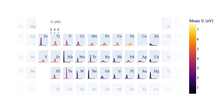
(a) Hubbard $U$ Periodic Table

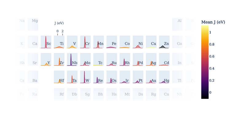
(b) Hund $J$ Periodic Table

Figure 1: Periodic table of Hubbard $U$ and Hund $J$ values computed for representative set of transition metal oxides. The color map indicates the mean value computed for each element over each material. The materials used in the creation of these periodic tabled were selectively chosen: noting that many databases, including the ICSD, contain a growing number of hypothetical materials which may or may not be realizable, we selected materials that are well-studied and exhibit more than two ICSD IDs each. Furthermore, to remove cross-correlations between magnetic elements, we also require that these compounds only contain a single $d$-block element (occupying a single symmetrically-equivalent site) with no $f$-block species. Ultimately this data corresponds to the $U$ and $J$ values for over 800 materials, and are distributed over the transition metal species. A more detailed table containing data on the distribution of values is included in Appendix C. The plotted distributions of $U$/$J$ values are generated using a Gaussian kernel-density estimator implemented in scipy [55].

Table 1: Comparison of computed $U_{\text{eff}}$ in the present work with values used by the Materials Project [38, 31].

element	mean $U_{\text{eff}}$ (eV)	$U_{\text{eff}}^{\text{MP}}$ (eV)	diff. (eV)
Co	4.430 $\pm$ 1.474	3.32	1.110
Cr	2.425 $\pm$ 0.472	3.7	-1.275
Fe	4.108 $\pm$ 1.322	5.3	-1.192
Mn	4.135 $\pm$ 0.724	3.9	0.235
Mo	1.911 $\pm$ 0.318	4.38	-2.469
Ni	5.258 $\pm$ 0.773	6.2	-0.942
V	3.060 $\pm$ 0.673	3.25	-0.190
W	1.461 $\pm$ 0.218	6.2	-4.739

III.1 Periodic table sample set

Figure 1 displays two periodic tables containing the distributions of computed Hubbard $U$ and Hund’s $J$ values for each transition metal element (and oxygen) computed for different structures within the database. In Table 1, values obtained in this study are listed alongside the standard $U$ values employed by the Materials Project [38, 31]. Those values were determined using the procedure outlined by Wang et al. [56] which finds a $U$ value that minimizes the error in formation energy for several representative redox couples. Due to the limited amount of experimental data available, these $U$ values are determined with only experimental data from a single redox couple (Co, Cr, Mo, Ni, and W) or two redox couples (Fe, Mn, and V). Therefore, it is possible or likely that these $U$ values are not appropriate for a more general system containing these elements. Nevertheless, the MP $U$ values are found to be the same as the $U$ values in the present work within the standard deviation for most elements (Co, Fe, Mn, and V) or slightly outside the value in the present work (Ni). Exceptions are Cr, Mo, and W, with the largest, notable discrepancy of 4.739 eV for W.

To evaluate the impact of these discrepancies, compounds containing W from a dataset of experimental formation energies [57] used by the Materials Project were taken and relaxed using the new $U_{\text{eff}}$ value for W from the present work but with all other calculation settings kept consistent with standard Materials Project settings, to obtain a new set of computed energies. These energies substantially lowered the correction introduced in Ref. 57 for W from -4.437 eV/atom to 0.12 eV/atom, suggesting that the newer $U_{\text{eff}}$ is indeed more appropriate for the calculation of formation energies.

Table 2: Computed range of $U$, $J$, and $U_{\text{eff}}$ values compared with reported $U_{\text{eff}}$ on the Materials Project (MP) [38], as well as the MP literature [31]. Each mean value has an associated standard deviation indicated after the “$\pm$.”

	mean	mean	mean	reported	reported
	computed	computed	computed	MP [38]	range [31]
Species	$U$ (eV)	$J$ (eV)	$U_{\text{eff}}=U-J$ (eV)	$U_{\text{eff}}$ (eV)	$U_{\text{eff}}$ (eV)
Mn-$d$	4.953 $\pm$ 0.635	0.520 $\pm$ 0.156	4.433 $\pm$ 0.654	3.9	3.60 – 5.09
Fe-$d$	4.936 $\pm$ 0.700	0.177 $\pm$ 0.367	4.759 $\pm$ 0.790	5.3	3.71 – 4.90
Ni-$d$	5.622 $\pm$ 1.221	0.399 $\pm$ 0.434	5.223 $\pm$ 1.296	6.2	5.10 – 6.93
O-$p$	10.241 $\pm$ 0.910	1.447 $\pm$ 0.171	8.794 $\pm$ 0.926	N/A	N/A

We stress that these values are not transferable to other studies, which use DFT implementations in other codes. Quantum ESPRESSO and Abinit use localized projections that are different from the projector augmented wave (PAW) method implemented in VASP [32].

III.2 Focused study on Mn-$d$, Fe-$d$, Ni-$d$, and O-$p$, including the reason for large O-$p$ Hubbard $U$ values

We now present a more detailed study on materials containing Mn-$d$, Fe-$d$, Ni-$d$, and O-$p$ Hubbard sites. For these systems, the distributions of the computed Hubbard $U$ and Hund $J$ values are provided in Figure 2. The variations in $U$ and $J$ values calculated for these three species is immediately apparent, with a range on the order of approximately 1 to 2 eV. These distributions reflect the intrinsic screening environment dependence of the calculated value for a given element. At this point, we note only their apparently universal unimodality (single peak) and the near-general decrease in $U$ with chemical period within a given group, however we will return presently to a more physically and chemically motivated observation. In Table 2 we list for comparison the $U$ values currently used in Materials project (fitted empirically) as well as a range of $U$ values found for a set of spinels and olivines by Zhou and co-workers (calculated via self-consistent linear response) [31].

We find that O-$p$ exhibits the largest associated Hubbard $U$ value of approximately 10 eV, which agrees with the linear response results from a previous study using a different code and somewhat different linear-response formalism [5]. While large oxygen Hubbard $U$ values may seem surprising within a strongly correlated materials context, it has become more accepted in recent years within first-principles solid-state chemistry that oxygen 2p orbitals can warrant, both by direct calculation and by necessity (when resorting to fitting), a remarkably high $U$ value in DFT+$U$.

We will now attempt to motivate and explain this phenomenon. We note from the outset that the element projector orbital profile plays a complicating role in the following analysis. In general, we observe that the diagonal elements of the $\chi_{0}$ non-interacting response matrix are of roughly the same magnitude for both TM-$d$ and O-$p$ sites. The non-self-consistent response can be interpreted as the response due to non-interacting response effects at a site due to its surroundings [10], and thus it can be understood as a property primarily of the environment of the atom under scrutiny. Then, unless screening is very short ranged as it may be in a very wide-gap insulator, this quantity may be said to be somewhat similar, on average, for metal and oxygen ions in an oxide. Thereby, the chemical trends in the Hubbard $U$ arise mostly in the interacting response.

Next, we note that the O-$p$ interacting response $\chi$ tends to be less than half of that of the interacting TM-$d$ response. This indicates that $-\chi^{-1}=d^{2}E/dn_{I}^{2}$, the curvature of the total energy versus occupation, $n_{I}$, is greater for O-$p$ states. This greater curvature versus occupation can be explained, we propose, in terms of known trends in the chemical hardness, i.e., the second chemical potential, i.e, the derivative of the chemical potential with respect to total charge at fixed external potential. We note, in passing, that some authors choose define the chemical hardness as half of that for historical reasons, but we suppress that here. Specifically, we can focus on the discretized (three-point) approximation to the global chemical hardness [58], namely

$$\nu {}\equiv d^{2}E/dN^{2}\approx E\left(N-1\right)-2E\left(N\right)+E\left(N+1\right)$$

$${}=\left[E\left(N+1\right)-E\left(N\right)\right]-\left[E\left(N\right)-E\left(N-1\right)\right]$$

$${}\equiv E_{i}-E_{a}\equiv E_{g},$$ (12)

which is nothing but the fundamental band-gap. This is a quantity that has been tabulated many times, and using the results of Ref. 59 we find that for atomic oxygen its value is $11.2$ eV, compared to that of the transition metal atoms, where it ranges from $5.8$ eV (Ti & Zr) to $8.0$ eV (Mn) if we exclude the often problematic zinc group, where it reaches $11.6$ eV. This mirrors and explains the observed relatively large first-principles Hubbard $U$ value for oxygen 2p states predicted in this and several previous studies.

Ultimately, we conclude that the Hubbard $U$ may be interpreted as the subspace-projected, environment screened chemical hardness, and more precisely as only the interaction (e.g., Hartree, exchange, correlation, and perhaps other terms like implicit solvent and PAW potential) part of that. It is in the interaction part that most of the chemical trends appear to arise in practice. For subspaces projecting heavily at both band-edges, as in normal DFT+$U$ practice, the $U$ clearly inherits chemical trends from the chemical hardness (fundamental gap) of the atom that it resides upon. This is higher for a higher atomic ionization energy $E_{i}$ (that of oxygen is generally around twice that of transition metals) and higher also for a more negative electron affinity $E_{a}$ (that of oxygen is more negative than that of most but not all transition metals). By and large, both quantities are well known to increase in magnitude as we move ‘up and right’ in the periodic table, and this same broad trend is reflected in our periodic table of Hubbard $U$ values.

When a DFT+$U$ subspace projects only onto one or other band edge, as seems more commonly the case for charge-tranfer insulators, then then the trend in only one of the ionization energy and electron affinity will be very relevant to the trends in $U$. In the case of oxygen 2p orbitals projectors, due to the electronegativity of oxygen typically there will be little weight at the conduction band edge, and so it is the (particularly clear) trend in ionization energy that drives the relatively large $U$ value for oxygen. Indeed, if this argument holds then one would guess that the oxygen 2p $U$ value is roughly twice that of an average transition-metal d subspace, which turns out to be the case from first principles linear response.

The Hund’s $J$, within the present formalism, may be interpreted as an analogue for the spin degree of freedom, and specifically as minus (by a convention thought to originate with Ising) the interaction part of the subspace-projected, environment screened spin-hardness, even the global atomic version of which [60] has been a much less thoroughly studied quantity. The effect of choosing whether these subspace charge (spin) hardness quantities, the $U$ and $J$, are calculated in a fully relaxed manner, or with with a simulated fixed spin (charge), is explored in our comparison between conventional (scaled) and constrained (simple) spin-polarized linear response, respectively, below.

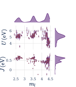
(a) Mn-$d$

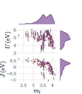
(b) Fe-$d$

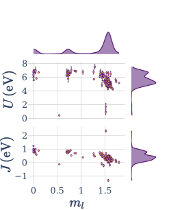
(c) Ni-$d$

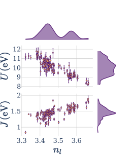
(d) O-$p$

Figure 2: Distributions of Hubbard $U$ and Hund $J$ values computed using the linear response method; For the sub-figures (a), (b), and (c) that correspond to $d$-electron TM site corrections, the $U$ and $J$ values are plotted against the DFT (no +$U$+$J$ correction) computed site magnetic $m_{l}$, where $m_{2}$ and $m$-$d$ are equivalent because $d$ occupations have a corresponding $l=2$ angular momentum quantum number. The O-$p$ $U$ and $J$ values in sub-figure (d) are plotted against $n_{l}$ ($n_{1}$ or $n$-p) total site occupations. The number of samples for on-site correction values for Mn-$d$, Fe-$d$, Ni-$d$, and O-$p$ are 285, 248, 149, and 206, respectively.

In order to explore trends in the distribution of $U$ and $J$ values, we have plotted these on-site corrections in scatter plots within Figure 2. These plots illustrate the relationship between $U$ and $J$ values with respect to site occupations. For transition metal species, we plot $U$ and $J$ versus $m_{l=2}$, the “$d$” component of the projected moment, $m$, denoted as “$m_{l=2}$.” These moment values are those output by VASP as the difference of up and down spin site occupancy numbers computed using PAW site-projection operators. Because the oxygen atoms do not have an associated magnetic moment, we plot O-$p$ Hubbard $U$ and Hund $J$ versus $n_{l=1}$ occupations on oxygen sites.

We should stress that the values of “$m_{l}$” and “$n_{l}$” are only computed from the calculation without the $+U$ correction. One reason for using the bare PBE computed $m_{l}$ and $n_{l}$ is that these occupations should be independent from the applied Hubbard $U$ or Hund $J$ values. This would offer the “bare” $m$, as well as $n$, as a possible predictors of $U$ and $J$ values. However, it is important to note that these occupations could change significantly with applied $U$ and $J$ values [5, 61, 62].

There is an apparent clustering of data points at different on-site $m_{l}$ magnetizations in Figures 2a, 2b, and 2c. This grouping at different on-site magnetization values is most likely due to different spin and charge states dependent on the underlying chemistry. We also observe a larger range of $U$ and $J$ values for higher values of $m_{l}$, which is due to the coupling between highly spin-polarized states to on-site Coulomb screening for TM species. As would be expected, we see similar trends for $J$, a measure of the screened interaction between spin channels.

For the Mn-$d$ and Ni-$d$ distributions in Figures 2a and 2c, a stark clustering of data-points is evident at particular intervals of $m_{l=2}$. In both cases, the clusters that lie at the associated maximum computed $m_{l}$ fall off and exhibit a negative slope trend with the magnitude of the site moment. This is likely due to the fact that $m_{l}$ is highly dependent on the local chemical environment, which will govern the energy curvature over spin occupations, which is directly related to $U$ and $J$ within linear response [4]. The clear trend for the manganese may be due to the strong tri-modal distribution of Mn magnetic moments seen in Figure 1 of Ref. 48. The “stable” magnetic configurations from this study were used in the LR analysis, therefore a similar statistical distribution should hold for the subset of structures used in this LR analysis.

The trends of the data points for Hubbard $U$ and Hund $J$ values in Figure 2d appear to show a downward trend for $U$ versus $p$-occupation numbers, $n_{l=1}$, and a slower, upward trend for $J$ values versus $n_{l=1}$. We expect that the $n_{l=1}$ occupations will be strongly dependent on the oxidation/reduction state of oxygen atoms. Due to the nature of TM-O bonding in these oxides, and their generally greater electronegativity, the oxygen atoms will tend to maximize their valence. Therefore, building on the previous explanation of the magnitude of O-$p$ $U$ values based on chemical hardness and specifically the more relevant ionization potential component of that, the higher electron count for oxygen corresponds to a lower ionization potential, and therefore to a reduced Hubbard $U$, as observed.

In an attempt to more robustly tease apart these observed trends, we performed a rudimentary random forest regression test on the data set, ultimately in an attempt to predict the on-site corrections $U$ and $J$ from the input crystal structures and site properties. We used the random forest regression algorithm as implemented in scikit-learn. The input quantities supplied to the random forest regressor consisted of the corresponding PBE-computed $m_{l}$ and $n_{l}$ - without on-site corrections, as well as the oxidation state estimated using the bond-valence method [63], and finally a selection of relevant site featurizers provided by the matminer Python package [64]. Unsurprisingly the $U$ and $J$ values appeared to be the most sensitive to the magnetic moment magnitude, $m=n_{\uparrow}-n_{\downarrow}$, and site occupation, $n=n_{\uparrow}+n_{\downarrow}$. This is in accordance with what would be expected from the dependence on the Hubbard $U$ values on spin and charge state [61, 62]. However, these features proved to be insufficient to accurately predict $U$ and $J$.

Most of the matminer site featurizers were tested as input to the random forest regression model. Ewald energy and Voronoi site featurizers had the greatest associated importance metric [64], second to $m_{l}$. However, the associated importance values of these featurizers were still less then the on-site magnetization, $m_{l}$. Additionally, the oxidation states calculated using the bond valence method (BVM) [63] were also included as input to the model. These guessed oxidation states are also used as input for the Ewald site featurizer. For learning trends across different atomic species, the atomic number of the associated element was also supplied. Additionally, we tested the orbital field matrix (OFM) features as formulated by [65, 66]. The OFM encodes the orbital character of the surrounding chemical environment. For more information on this method please refer to Ref. 65. The OFM functionality is not implemented in matminer or pymatgen. We were motivated to test the vectorized OFM by the chemical intuition that on-site Hubbard $U$ and Hund $J$ values are very sensitive to the local chemical environment. Additionally, the OFM has demonstrated success in predicting DFT-computed magnetic moments in the past [65]. Furthermore, the OFM nearest-neighbor contributions are weighted according to the geometry of the Voronoi cell, which could possibly provide information beyond the relative importance of the Voronoi matminer featurizer. However, the on-site magnetization for Mn, Fe, and Ni, respectively, had an importance of at least ten percent more than any of the other local chemical environment descriptors.

The correlation between on-site corrections and projected site moments is not surprising. After all, previous studies have explored the connection between charge states of transition metal species and the integrated net spin calculated from DFT [67, 68, 69]. The integrated atomic spin moment can be directly linked to the charge state of transition metal species via magnetochemistry rules. In fact, recent studies show that the magnetic moment is often the most convenient and reliable indicator of charge states [67].

III.2.1 Conventional vs. constrained linear response

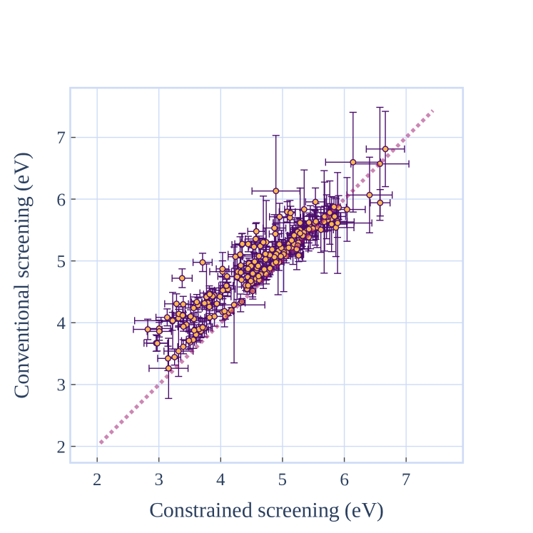
Figure 3: Comparison between the conventional and constrained approaches for calculating Hubbard $U$ values for Fe-$d$ Hubbard sites.

In introducing the linear response theory in Section II.2, we mentioned that there are two possible schemes for computing $U$ and $J$: “conventional” and “constrained” linear response, where in the latter case the linear response is performed in such a way that the magnetic moment (occupation) is held fixed while measuring the curvature with respect to the occupation (magnetic moment). While arguments can be made as to theoretically which approach is the most valid (a topic which is the subject of ongoing research), this dataset presents an opportunity to evaluate how much this choice will practically affect the resulting Hubbard and Hund’s parameters.

For the majority of the computed $U$ and $J$ values using these two methods, the difference between the two strategies fell within their computed uncertainty. However, we observed a significant deviation from $y=x$ behavior for the computed $U$ values for iron Hubbard $U$ values shown in Figure 3. The width of this distribution is greater than 1 eV for $U$ in some regions, which is enough to affect computed physical properties [4, 61].

III.2.2 Dependence on structure and magnetic state

For some input magnetic structures, the magnetic configuration changed while applying the on-site potentials during the linear response analysis. Our hypothesis is that the input magnetic structure corresponds to a local minimum configuration, or possibly a metastable state. Therefore, in our analysis, we screen out these structures with the intent that these systems will be studied in the future using a self-consistent approach to calculating on-site corrections.

In order to test the sensitivity of $U$ and $J$ values to the input structure, we perform a self-consistent linear response study of antiferromagnetic NiO, which is provided in the Supplementary Information. Each iteration consists geometry optimization of cell shape, followed by a linear response calculation of $U$ and $J$ values. These on-site correction values are then used in the next subsequent geometry optimization step. Self-consistency is achieved once the $U$ and $J$ values fall within their corresponding uncertainty values. Starting from the input structure — which was optimized using the current default Materials Project $U$ values [38] — convergence was achieved after only two iterations.

It has been well established in previous studies that $U$ values should be computed self-consistently with geometry optimization [61]. As demonstrated from the experiments with antiferromagnetic NiO in the Supplementary Information section, the Hund $J$ values should be calculated self-consistently, in addition to Hubbard $U$ values. In this self-consistency study, $J$ had the largest associated change over convergence relative to the value itself. Due to the coupling between Hund $J$ and magnetic exchange [22], it is possible that both magnetic and structural features should be included in the self-consistency cycle. Within the atomate framework, it would be possible to incorporate a workflow that wraps the workflow developed in this study, in order to alternate linear response calculations with geometry relaxation until self-consistency is achieved.

III.3 Case study: LiNiPO4

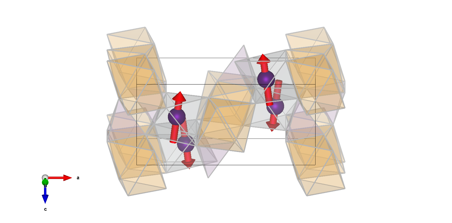
Figure 4: Olivine crystal structure of LiNiPO4 with magnetic atoms visible. Taken from [35] via the Bilbao MAGNDATA database [70, 35]. The purple atoms correspond to magnetic nickel atoms. The oxygen octahedra surrounding lithium atoms are indicated in orange, where the grey oxygen octahedra surround nickel sites.

We now present a detailed study on the olivine LiNPO4, designed to test the results produced by the linear response workflow. Previous GGA$+U$ and GGA+$U$+$J$ studies have attempted to reproduce the experimentally-observed spin-canting structure and unit cell shape as shown in Figure 4 [19, 31, 35].

We calculated $U$ and $J$ for this system via spin-polarized linear response. The spin-polarized linear response method introduced in Section II.2 can be generalized to noncollinear DFT using the relationship between spin-density occupations and the magnitude of the magnetic moment: $n_{\uparrow}=\frac{1}{2}\left(n+|\vec{m}|\right)$ and $n_{\uparrow}=\frac{1}{2}\left(n-|\vec{m}|\right)$ [21]. For comparison, we also performed a collinear calculation, where the magnetic configuration for LiNiPO4 was obtained by projecting the canted noncollinear structure shown in Figure 4 along the $z$-direction. In addition to one unit cell of the the collinear antiferromangetic (AFM) configuration, a linear response analysis was performed on a 1$\times$2$\times$2 supercell. Table 3 summarizes the results of the computed Hubbard $U$ and Hund $J$ values. From this table, it is evident that the $U$ value is significantly smaller in magnitude with the inclusion of spin-orbit coupling. A possible justification for this behavior is the introduction of orbital contributions to the total localized magnetic moments with the inclusion of spin-orbit coupling [71, 22].

Table 3: Hubbard and Hund results for Ni-$d$ in LiNiPO₄ (Atom-wise screening)

cell	magnetism	$U$ (eV)	$J$ (eV)
$1\times 1\times 1$	collinear	5.43 $\pm$ 0.16	0.38 $\pm$ 0.07
$1\times 2\times 2$	collinear	5.44 $\pm$ 0.24	0.54 $\pm$ 0.07
$1\times 1\times 1$	non-collinear	5.09 $\pm$ 0.15	0.42 $\pm$ 0.05

III.3.1 Canting angle exploration

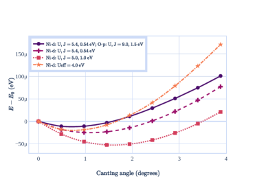
(a) Computed energy versus constraining canting angle

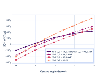
(b) Effective constraining field versus constraining canting angle

Figure 5: (a) Computed relative energy and (b) $x$-component of effective constraining local magnetic field for various Hubbard and Hund on-site corrections applied to the Ni-$d$ and O-$p$ manifolds.

In order to explore the canting angle experimentally observed for LiNiPO4 [35], we calculated the energy as a function of constrained canting angle. The noncollinear magnetic constraints were performed in VASP in accordance with the method developed by Ma and Dudarev [72]. We used the experimentally derived spin canted structure as a reference provided by the Bilbao Crystallographic Server, as shown in Figure 4 [70, 35]. The energy versus canting angle curve is shown in Figure 5a. We found that the stable canting direction is in the opposite direction to the experimentally measured canting angle. However, this discrepancy with experiment was limited to the canting direction; the computed stable magnetic structure still obeyed the symmetry of the Pnm’a magnetic space group.

Similarly to the work by Bousquet and Spaldin [19], we observe an increasing canting angle with Hund $J$ value. Interestingly, adding a $U$ and $J$ correction to O-$p$ results in a slightly decreased stable canting angle. However, we find that in all cases, the computed stable canting angle is significantly less than the experimentally measured canting angle of 7.8 degrees [35].

The constraining effective site magnetic field, $\vec{H}^{\text{eff}}_{i}$, can be described as the following

$$\vec{H}^{\text{eff}}_{i} =2\lambda\left[{\vec{M}}_{i}-{\hat{M}}_{i}^{0}\left({\hat{M}}_{i}^{0}\cdot{\vec{M_{i}}}\right)\right]$$ (13)

where ${\vec{M}}_{i}$ are the integrated magnetic moments at site $i$, and ${\hat{M}}_{i}^{0}$ are the unit vectors pointing in the individual site constraining directions [72]. The $x$ component of the constraining field (in the direction of canting), ${H}^{\text{eff}}_{i,x}$, is plotted versus the constraining angle in Figure 5b. We see that where ${H}^{\text{eff}}_{i,x}$ changes sign corresponds to the minimum of Figure 5a.

III.3.2 Effect of $U$ and $J$ values on geometry optimization

Table 4: Lattice parameters, cell volume, and mean Ni-O bond length ($d$) of LiNiPO₄ canted structure for different Hubbard $U$ and Hund $J$ corrections

method	Ni-$d$ (eV)	O-$p$ (eV)	$a$ (Å)	$b$ (Å)	$c$ (Å)	volume (Å3)	$d$ (Å)
experiment			10.03	5.85	4.68	274.93	2.086 $\pm$ 0.044
PBE			10.09 (+0.6%)	5.92 (+1.1%)	4.72 (+0.9%)	282.09 (+2.6%)	2.099 $\pm$ 0.037
PBE$+U_{\text{eff}}$	$U_{\text{eff}}$ = 4	$U_{\text{eff}}$ = 0	10.14 (+1.1%)	5.92 (+1.1%)	4.73 (+1.0%)	283.71 (+3.2%)
		$U_{\text{eff}}$ = 7.5	10.07 (+0.4%)	5.87 (+0.3%)	4.69 (+0.3%)	277.56 (+1.0%)
PBE+$U$+$J$	$U$ = 5	$U$, $J$ = 0	10.15 (+1.2%)	5.92 (+1.1%)	4.73 (+1.0%)	284.19 (+3.4%)	2.108 $\pm$ 0.039
	$J$ = 1	$U$, $J$ = 9, 1.5	10.07 (+0.4%)	5.88 (+0.4%)	4.69 (+0.3%)	277.86 (+1.1%)	2.095 $\pm$ 0.043

While the addition of Hubbard and Hunds parameters go some way to addressing the canting angle of LiNiNO4, introducing these terms can also alter the geometry of the system. To explore this effect, we performed structural relaxations of the system with various combinations of Hubbard and Hund’s corrections. In each of these structural relaxation calculations, a maximum force tolerance was used of 10 meV/Å. All runs included spin-orbit coupling, and were constrained to the 7.8 degrees experimentally observed canting angle.

Table 4 lists the optimized unit cell parameters and volume, compared with the experimentally measured geometry [35]. For both the PBE+$U_{\mathrm{eff}}$ and PBE+$U$+$J$ schemes, adding corrections to the Ni-$d$ space worsens the geometry relative to the uncorrected PBE geometry (as earlier observed by Zhou and co-workers [31]. However, the further addition of corrections to the O-$p$ subspace reduces the errors by three-fold, resulting in geometries that are closest to experiment. This is similar to observations in other studies when applying corrections to O-$p$ subspaces [5]. We note that applying a +$J$ correction to non-magnetic O-$p$ states is unconventional. However, it should be stressed that the projected magnetic moments on LiNiPO4 remain just below 0.01 $\mu_{B}$, with and without on-site corrections to O-$2p$ states. Meanwhile, we can see that adding a $+J$ parameter does not significantly alter the cell parameters.

The Hubbard $U$ and Hund $J$ values used in this study of LiNiPO4 include those calculated using linear response, which are approximations of the values that are reported in Table 3. Additionally, we tested the Ni-$d$ $U$/$J$ values used in Ref. 19, in order to compare with previous computational studies of the magnetic structure of LiNiPO4.

III.3.3 Discussion on TM-O bond length versus U, J, and V corrections

Table 4 also presents the change in mean Ni-O bond length between nearest-neighbor pairs for various on-site corrections. For the Ni-O bond length it is the same story as for the cell parameters: applying $U$ and $J$ to the Ni-$d$ sites worsens the results relative to the PBE result, but by applying corrections to the O-$p$ channels we obtain bond lengths that are in closer agreement with experiment. In Ref. 5, some of us attempted to rationalize this trend in the computed bond length between transition metal species and oxygen anions and how it improves with the introduction of corrections to the O-$p$ subspace [5]. We suggested that when $+U$ is added to the Ni-$d$ subspace the resulting potential shift disrupts hybridization between the Ni-$d$ and O-$p$ orbitals, weakening the bonding between these two elements (and thus leading to bond lengthening). By applying corrections to the O-$p$ re-aligns these two subspaces and allows them to “re-hybridize”.

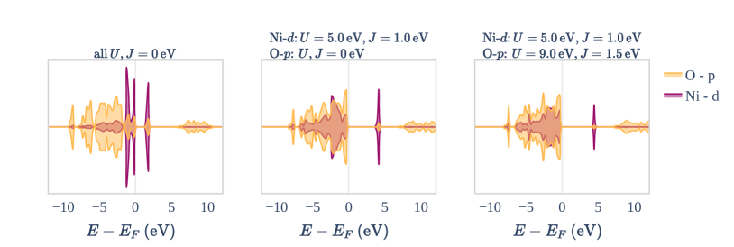
Figure 6: Projected electronic density of states for LiNiPO4 (calculated using experimental unit cell [35]) without Hubbard or Hund corrections applied, as well as $+U$ and $+J$ applied to Ni-$d$ channels, and both Ni-$d$ and O-$p$ states, respectively.

In an attempt to more thoroughly explore this reasoning, Figure 6 provides a comparison for the projected density of states (DOS) of LiNiPO4 for PBE and PBE+$U$+$J$ (with and without corrections to O-$p$). It is difficult to discern re-hybridization from DOS plots alone.

Without an explicit quantification of hybridization effects, we have added a derivation in the Supplementary Information that presents a mathematical expression of the forces acting on ions due to +$U$+$V$ corrections. This result is an extension of the theory put forth by Matteo Cococcioni in Chapter 4, Section 4.1 of Ref. 10. We argue that in quantifying the forces on TM-O bond lengths due to on-site corrections, it is possible to show that the force contributions due to both +$U^{\gamma}$ and +$V^{\gamma\gamma^{\prime}}$ can, and should, be treated on the same footing, where $\gamma$ and $\gamma^{\prime}$ correspond to atomic sites. It isn’t possible to definitively state the comparative magnitude, or sign, of these force contributions without additional calculations or simplifications based on physical intuition. However, the result suggests that the forces on TM-O bond-length due to O-$p$ $U$ values will have a comparative magnitude to the forces due to inter-site Coulomb corrections due to +$V$.

In the Supplementary Information, we further hypothesize the sign of these force contributions, starting from a DFT geometry-optimized structure without on-site corrections. Using these assumptions, which are based on computational trends in bulk TMOs, we conclude that both applying a +$U$ correction to the O-$p$ manifold and a +$V$ between TM and O states combine to mitigate the overestimation of TM-O bond length that arises when only applying +$U$ to localized states around the TM species.

IV Conclusions

This study provides a high-throughput atomate framework for calculating Hubbard $U$ and Hund’s $J$ values. Using the spin-polarized linear-response methodology [5], we generated a database of $U$ and $J$ values for over two thousand transition-metal-containing materials. This enabled the creation of a “periodic table” of $U$ and $J$ values, where for each element we observe a distribution of Hubbard $U$ and Hund’s $J$ values. These distributions exhibited clustering depending on the corresponding $m_{l}$ and $n_{l}$ values, but these quantities alone do not prove sufficient to predict the Hubbard and Hund’s parameters.

In addition to +$U$+$J$, inter-site +$V$ corrections will also contribute to electronic properties. In order to investigate inter-site screening effects on the resulting $U$/$J$ values, we performed a small supercell scaling study for the full screening linear response analysis for NiO, in addition to the conventional, atom-wise, screening. This exploration can be found in the Supplementary Information, and the details of the full screening matrix inversion can be found in Appendix A. We found that the full matrix inversion is much more sensitive to the size of the unit cell compared to the conventional, atom-wise screening. The theoretical reasons for this phenomenon will be an interesting pursuit for future studies, in addition to the effect of the corresponding $V^{\gamma\gamma^{\prime}}$ values on the DFT+$U$(+$J$)+$V$ ground-state. Currently, VASP does not have +$V$ corrections implemented.

In order to test the validity of the linear response implementation, we explored the spin-canting noncollinear magnetic structure and unit cell shape of LiNiPO4, and compare the results with previous experimental [35] and computational [19, 31] studies. Similarly to Bousquet and Spaldin [19], we observed that the computed stable canting angle was less than 50% of the experimentally measured canting angle of nickel magnetic moments in olivine LiNiPO4, for Ni-$d$ Hund $J$ values up to 2 eV. We also observed a large sensitivity to the canting angle and Hund $J$ values. This confirms that Hund $J$ values are crucial for exploring the properties of transition metal oxides which exhibit a noncollinear magnetic structure. In addition to the canting structure of LiNiPO4, we also presented the relaxed unit cell shape for various Hubbard $U$ and Hund $J$ corrections. While applying a +$U$+$J$ correction to Ni-$d$ resulted in increased disagreement with experimentally measured unit cell parameters [31], applying an on-site Hubbard/Hund correction to O-$p$ occupancies greatly improved the agreement of unit cell shape with experiment [35]. This finding reinforces the importance of including a +$U$+$J$ correction to oxygen sites in order to resolve the accurate bonding behavior between transition metal species and neighboring oxygen atoms.

CRediT Taxonomy

We highlight the author contributions to this study using the CRediT taxonomy. Guy C. Moore: Conceptualization, Methodology, Software, Validation, Formal analysis, Investigation, Data Curation, Writing - Original Draft, Writing - Review & Editing, Visualization Matthew K. Horton: Conceptualization, Software, Validation, Investigation, Writing - Review & Editing, Visualization, Project administration Alexander M. Ganose: Software, Writing - Review & Editing Edward Linscott: Methodology, Validation, Formal analysis, Investigation, Writing - Review & Editing David D. O’Regan: Methodology, Validation, Formal analysis, Investigation, Writing - Review & Editing Martin Siron: Software, Writing - Review & Editing Kristin A. Persson: Writing - Review & Editing, Supervision, Project administration.

Appendix A Screening matrix inversions

Below are the matrix representations of the response matrices at each level of screening outlined by Linscott and others for a system with two Hubbard sites [5].

Point-wise $1\times 1$ screening:

$$\chi^{-1} =\begin{pmatrix}1/\chi_{11}&0\\ 0&1/\chi_{22}\\ \end{pmatrix}$$ (14)

Atom-wise (conventional) $2\times 2$ screening:

$$\chi^{-1} =\begin{pmatrix}\chi_{11}&\chi_{12}\\ \chi_{21}&\chi_{22}\\ \end{pmatrix}^{-1}$$ (15)

We can extend this formalism to the multiple site (multi-site) responses by considering the response matrix for two sites, $\chi_{ij}$, where $i$ and $j$ are the site indices.

Point-wise screening:

$$\chi^{-1} =\begin{pmatrix}\begin{pmatrix}1/\chi^{\uparrow\uparrow}_{11}&0\\ 0&1/\chi^{\downarrow\downarrow}_{11}\\ \end{pmatrix}&\text{\Large 0}\\ \text{\Large 0}&\begin{pmatrix}1/\chi^{\uparrow\uparrow}_{22}&0\\ 0&1/\chi^{\downarrow\downarrow}_{22}\\ \end{pmatrix}\\ \end{pmatrix}$$ (16)

Atom-wise (conventional) screening:

$$\chi^{-1} =\begin{pmatrix}\begin{pmatrix}\chi^{\uparrow\uparrow}_{11}&\chi^{\uparrow\downarrow}_{11}\\ \chi^{\downarrow\uparrow}_{11}&\chi^{\downarrow\downarrow}_{11}\\ \end{pmatrix}^{-1}&\text{\Large 0}\\ \text{\Large 0}&\begin{pmatrix}\chi^{\uparrow\uparrow}_{22}&\chi^{\uparrow\downarrow}_{22}\\ \chi^{\downarrow\uparrow}_{22}&\chi^{\downarrow\downarrow}_{22}\\ \end{pmatrix}^{-1}\\ \end{pmatrix}$$ (17)

Full screening:

$$\chi^{-1} =\begin{pmatrix}\chi^{\uparrow\uparrow}_{11}&\chi^{\uparrow\downarrow}_{11}&\chi^{\uparrow\uparrow}_{12}&\chi^{\uparrow\downarrow}_{12}\\ \chi^{\downarrow\uparrow}_{11}&\chi^{\downarrow\downarrow}_{11}&\chi^{\downarrow\uparrow}_{12}&\chi^{\downarrow\downarrow}_{12}\\ \chi^{\uparrow\uparrow}_{21}&\chi^{\uparrow\downarrow}_{21}&\chi^{\uparrow\uparrow}_{22}&\chi^{\uparrow\downarrow}_{22}\\ \chi^{\downarrow\uparrow}_{21}&\chi^{\downarrow\downarrow}_{21}&\chi^{\downarrow\uparrow}_{22}&\chi^{\downarrow\downarrow}_{22}\\ \end{pmatrix}^{-1}$$ (18)

We note that it is important when performing a linear response calculation to construct a $2N\times 2N$ response matrix where $N$ is the number of Hubbard sites (or $N\times N$ in the case of non-spin-polarized linear response). For bulk systems often several Hubbard sites will be equivalent, and one can save computational time by performing linear response calculations for the set of inequivalent sites, and then populating the response matrix for all equivalent Hubbard-site pairs.

Appendix B Post-processing & uncertainty quantification

In order to extract the response matrices from the raw DFT data, curve fitting was performed using a least-squares polynomial fit implemented in numpy [73]. The uncertainty associated with each computed slope was obtained from the covariance matrix produced as a result of the least-squares fit. These uncertainty values were then utilized to determine the errors associated with the Hubbard $U$ and Hund $J$ values. The error quantification was performed by computing the propagation of uncertainty based on the Jacobian of each scaling formula for Hubbard $U$ and Hund $J$. This method for error propagation is general to multiple levels of screening between spin, site, and orbital responses.

We begin by considering the following screening matrix introduced in Equation 11, from which Hubbard $U$ and Hund $J$ values are derived [5]

$$f_{ij}=\left(\chi_{0}^{-1}-\chi^{-1}\right)_{ij}$$

Derivatives of the $\chi^{-1}$ matrix with respect to individual $\chi_{kl}$ can be obtained by the following relation:

$$\frac{\partial}{\partial\chi_{kl}}\left(\chi^{-1}\right) =-\chi^{-1}\left(\frac{\partial}{\partial\chi_{kl}}\chi\right)\chi^{-1}$$

$$\text{where }\frac{\partial}{\partial\chi_{kl}}\left\{\chi\right\}_{ij}=\begin{cases}1&\text{if }kl=ij\\ 0&\text{otherwise}\end{cases}$$

$$\frac{\partial}{\partial\chi_{kl}}\left\{\chi^{-1}\right\}_{ij} =-\left\{\chi^{-1}\right\}_{ik}\left\{\chi^{-1}\right\}_{lj}$$ (19)

Using this fact, it is possible to obtain the full Jacobian of $f$ with respect to response $\chi$ matrices which can be used to obtain the covariance uncertainty matrix associated with the elements of $f_{ij}$, to a first-order expansion of $f_{ij}$ [74]

$$\bm{\Sigma}_{f} =\bm{J}_{\chi_{0}}\bm{\Sigma}_{\chi_{0}}\bm{J}_{\chi_{0}}^{T}+\bm{J}_{\chi}\bm{\Sigma}_{\chi}\bm{J}_{\chi}^{T}$$ (20)

where $\bm{\Sigma}_{f}$ is a $N^{2}\times N^{2}$ matrix ($f$ is $N\times N$). Each element of $\bm{\Sigma}_{f}$, $\left\{\Sigma_{f}\right\}_{ij,kl}$, corresponds to the covariance between $f_{ij}$ and $f_{kl}$ matrix elements. $\bm{\Sigma}_{\chi}$ and $\bm{\Sigma}_{\chi_{0}}$ are the covariance matrices for each $\left\{\chi\right\}_{kl}$ and $\left\{\chi_{0}\right\}_{kl}$, and the diagonal elements are populated using the squared uncertainty values associated with the slopes fit to the response data. In addition, $\bm{J}_{\chi}$ and $\bm{J}_{\chi_{0}}$ are the symbolically derived Jacobians corresponding to each response value, as proposed in Equation 19. Assuming that the individual elements of $\chi$ and $\chi_{0}$ are independent, we can assume that $\bm{\Sigma}$ covariance matrices are diagonal in order to make the following simplification:

$$\sigma^{2}(f_{ij}) =\sum_{kl}\left(\frac{\partial}{\partial\left\{\chi_{0}\right\}_{kl}}f_{ij}\right)^{2}\sigma^{2}(\left\{\chi_{0}\right\}_{kl})$$

$$\quad+\sum_{kl}\left(\frac{\partial}{\partial\left\{\chi\right\}_{kl}}f_{ij}\right)^{2}\sigma^{2}(\left\{\chi\right\}_{kl}),$$ (21)

where $\sigma^{2}(f_{ij})$, $\sigma^{2}(\left\{\chi_{0}\right\}_{ij})$, and $\sigma^{2}(\left\{\chi\right\}_{ij})$ correspond to the diagonal elements of $\bm{\Sigma}_{f}$, $\bm{\Sigma}_{\chi_{0}}$, and $\bm{\Sigma}_{\chi}$, respectively.

With the established expression for the uncertainty values of $f$ in Equation 21, we can express the squared uncertainty of $U$, for an atomic site $\gamma$, in the next level of uncertainty propagation,

$$\sigma^{2}(U^{\gamma}) =\sum_{\sigma,\sigma^{\prime}}\left(\frac{\partial}{\partial f^{\sigma\sigma^{\prime}}_{\gamma\gamma}}G_{U}(f_{\gamma\gamma})\right)^{2}\sigma^{2}(f^{\sigma\sigma^{\prime}}_{\gamma\gamma}).$$ (22)

Equation 22 can be extended to an expression of the squared uncertainty of Hund $J$, where $G_{U}$ and $G_{J}$ are functions of 2$\times$2 sub-matrices along the diagonal of $f$, as introduced in Equation 11, and depend on the different scaling schemes introduced in Ref. 5.

Appendix C Details of the data behind the periodic tables

Table 5: The mean and standard deviation ($\sigma$) in the $U$ and $J$ parameters used in the periodic tables of Figure 1, alongside the number of samples $N$.

element	$U$			$J$
	mean	$\sigma$	$N$	mean	$\sigma$	$N$
Mn	4.710	0.707	94	0.575	0.157	97
Fe	4.545	0.674	78	0.437	1.137	122
V	3.909	0.404	68	0.849	0.538	108
Cu	7.590	0.728	51	1.117	1.083	71
Cr	2.982	0.464	51	0.557	0.089	61
Nb	0.529	0.107	47	0.193	0.054	39
Ti	4.737	0.428	45	0.705	0.861	62
Ta	3.688	0.130	34	0.628	0.079	37
W	1.846	0.213	33	0.385	0.045	33
Co	5.237	0.566	33	0.807	1.361	46
Ag	2.830	0.606	26	0.703	0.131	24
Re	0.598	0.172	26	0.255	0.089	27
Ni	5.847	0.704	25	0.589	0.320	33
Zr	4.382	0.269	24	0.740	0.069	23
Mo	2.431	0.230	21	0.520	0.220	28
Hg	0.620	0.226	21	0.288	0.271	22
Cd	0.350	0.327	19	0.609	0.614	5
Sc	2.506	0.210	16	0.543	0.070	16
Y	4.704	0.393	15	0.825	0.179	5
Pt	1.673	0.318	13	0.322	0.201	14
Os	1.855	0.448	10	0.361	0.087	11
Ru	2.972	0.548	10	0.504	0.292	24
Lu	0.449	0.065	9	0.292	0.072	8
Pd	3.608	0.407	8	0.620	0.106	10
Hf	3.733	0.299	8	0.812	0.122	8
Au	1.186	0.256	7	0.484	0.165	8
Zn	0.530	0.795	5	-0.105	0.433	17
Rh	1.616	0.201	5	0.406	0.065	5
Ir	1.868	0.288	5	0.352	0.283	14
Tc	2.956	0.100	3	0.980	1.247	9
Total			810			987

References

- Koch et al. [2012] E. Koch, F. Anders, and M. Jarrell, Correlated electrons: from models to materials, edited by E. Pavarini, Schriften des Forschungszentrums Jülich. Reihe modeling and simulation, Vol. 2 (Forschungszentrum Jülich GmbH Zenralbibliothek, Verlag, Jülich, 2012) p. getr. Paginierung, record converted from JUWEL: 18.07.2013.
- Langreth and Mehl [1983] D. C. Langreth and M. J. Mehl, Beyond the local-density approximation in calculations of ground-state electronic properties, Phys. Rev. B 28, 1809 (1983).
- Kohn and Sham [1965] W. Kohn and L. J. Sham, Self-consistent equations including exchange and correlation effects, Phys. Rev. 140, A1133 (1965).
- Cococcioni and de Gironcoli [2005] M. Cococcioni and S. de Gironcoli, Linear response approach to the calculation of the effective interaction parameters in the LDA+ method, Phys. Rev. B 71, 035105 (2005).
- Linscott et al. [2018] E. B. Linscott, D. J. Cole, M. C. Payne, and D. D. O’Regan, Role of spin in the calculation of Hubbard and Hund’s parameters from first principles, Phys. Rev. B 98, 235157 (2018).
- Anisimov et al. [1991] V. I. Anisimov, J. Zaanen, and O. K. Andersen, Band theory and Mott insulators: Hubbard instead of Stoner , Phys. Rev. B 44, 943 (1991).
- Anisimov et al. [1993] V. I. Anisimov, I. V. Solovyev, M. A. Korotin, M. T. Czyżyk, and G. A. Sawatzky, Density-functional theory and NiO photoemission spectra, Phys. Rev. B 48, 16929 (1993).
- Anisimov et al. [1997] V. I. Anisimov, F. Aryasetiawan, and A. I. Lichtenstein, First-principles calculations of the electronic structure and spectra of strongly correlated systems: The LDA + U method, J. Phys. Condens. Matter 9, 767 (1997).
- Pickett et al. [1998] W. E. Pickett, S. C. Erwin, and E. C. Ethridge, Reformulation of the LDA + U method for a local-orbital basis, Phys. Rev. B 58, 1201 (1998).
- Cococcioni [2012] M. Cococcioni, Chapter 4 - The LDA+ approach: A simple hubbard correction for correlated ground states, in [1], pp. 4.1–4.40, record converted from JUWEL: 18.07.2013.
- Kulik et al. [2006] H. J. Kulik, M. Cococcioni, D. A. Scherlis, and N. Marzari, Density Functional Theory in Transition-Metal Chemistry: A Self-Consistent Hubbard U Approach, Physical Review Letters 97, 103001 (2006).
- Himmetoglu et al. [2014] B. Himmetoglu, A. Floris, S. d. Gironcoli, and M. Cococcioni, Hubbard-corrected DFT energy functionals: The LDA+U description of correlated systems, International Journal of Quantum Chemistry 114, 14 (2014).
- Bajaj et al. [2017] A. Bajaj, J. P. Janet, and H. J. Kulik, Communication: Recovering the flat-plane condition in electronic structure theory at semi-local DFT cost, The Journal of Chemical Physics 147, 191101 (2017), publisher: American Institute of Physics.
- Bajaj and Kulik [2021] A. Bajaj and H. J. Kulik, Molecular DFT+U: A Transferable, Low-Cost Approach to Eliminate Delocalization Error, The Journal of Physical Chemistry Letters 10.1021/acs.jpclett.1c00796 (2021), publisher: American Chemical Society.
- Campo Jr and Cococcioni [2010] V. L. Campo Jr and M. Cococcioni, Extended DFT+U+V method with on-site and inter-site electronic interactions, Journal of Physics: Condensed Matter 22, 055602 (2010), arXiv: 0907.5272.
- Tancogne-Dejean and Rubio [2020] N. Tancogne-Dejean and A. Rubio, Parameter-free hybridlike functional based on an extended Hubbard model: DFT+U+V, Physical Review B 102, 155117 (2020).
- Lee and Son [2020] S.-H. Lee and Y.-W. Son, First-principles approach with a pseudohybrid density functional for extended Hubbard interactions, Physical Review Research 2, 043410 (2020).
- Dudarev et al. [1998] S. L. Dudarev, G. A. Botton, S. Y. Savrasov, C. J. Humphreys, and A. P. Sutton, Electron-energy-loss spectra and the structural stability of nickel oxide: An LSDA+U study, Phys. Rev. B 57, 1505 (1998).
- Bousquet and Spaldin [2010] E. Bousquet and N. Spaldin, dependence in the treatment of noncollinear magnets, Phys. Rev. B 82, 220402 (2010).
- Bultmark et al. [2009] F. Bultmark, F. Cricchio, O. Grånäs, and L. Nordström, Multipole decomposition of LDA+ energy and its application to actinide compounds, Physical Review B 80, 035121 (2009).
- Dudarev et al. [2019] S. L. Dudarev, P. Liu, D. A. Andersson, C. R. Stanek, T. Ozaki, and C. Franchini, Parametrization of LSDA+U for noncollinear magnetic configurations: Multipolar magnetism in \ceUO2, Physical Review Materials 3, 083802 (2019), arXiv: 1811.06864.
- Streltsov and Khomskii [2017] S. V. Streltsov and D. I. Khomskii, Orbital physics in transition metal compounds: new trends, Physics-Uspekhi 60, 1121 (2017), publisher: IOP Publishing.
- Mellan et al. [2015a] T. A. Mellan, F. Corà, R. Grau-Crespo, and S. Ismail-Beigi, Importance of anisotropic coulomb interaction in , Phys. Rev. B 92, 085151 (2015a).
- Georges et al. [2013a] A. Georges, L. d. Medici, and J. Mravlje, Strong correlations from Hund’s coupling, Annual Review of Condensed Matter Physics 4, 137 (2013a).
- Herper et al. [2017] H. C. Herper, T. Ahmed, J. M. Wills, I. Di Marco, T. Björkman, D. Iuşan, A. V. Balatsky, and O. Eriksson, Combining electronic structure and many-body theory with large databases: A method for predicting the nature of 4 states in Ce compounds, Physical Review Materials 1, 033802 (2017).
- Jain et al. [2011] A. Jain, G. Hautier, S. P. Ong, C. J. Moore, C. C. Fischer, K. A. Persson, and G. Ceder, Formation enthalpies by mixing GGA and GGA+U calculations, Physical Review B 84, 045115 (2011), publisher: American Physical Society.
- Yu et al. [2020] M. Yu, M. Yang, C. Wu, and N. Marom, Machine learning the Hubbard U parameter in DFT+U using Bayesian optimization, npj Computational Materials 6, 1 (2020), number: 1 Publisher: Nature Publishing Group.
- Albers et al. [2009] R. C. Albers, N. E. Christensen, and A. Svane, Hubbard-U band-structure methods, Journal of Physics: Condensed Matter 21, 343201 (2009).
- Elfimov et al. [2007] I. S. Elfimov, A. Rusydi, S. I. Csiszar, Z. Hu, H. H. Hsieh, H.-J. Lin, C. T. Chen, R. Liang, and G. A. Sawatzky, Magnetizing Oxides by Substituting Nitrogen for Oxygen, Physical Review Letters 98, 137202 (2007).
- Liechtenstein et al. [1995a] A. I. Liechtenstein, V. I. Anisimov, and J. Zaanen, Density functional theory and strong interactions: Orbital ordering in Mott-Hubbard insulators, Phys. Rev. B 52, R5467 (1995a).
- Zhou et al. [2004] F. Zhou, M. Cococcioni, C. A. Marianetti, D. Morgan, and G. Ceder, First-principles prediction of redox potentials in transition-metal compounds with LDA+U, Phys. Rev. B 70, 235121 (2004).
- Wang et al. [2016] Y.-C. Wang, Z.-H. Chen, and H. Jiang, The local projection in the density functional theory plus U approach: A critical assessment, The Journal of Chemical Physics 144, 144106 (2016).
- Ren [2019] X. Ren, Chapter 2 - The random phase approximation and its applications to real materials, in [85], pp. 2.1–2.27.
- Vaugier et al. [2012] L. Vaugier, H. Jiang, and S. Biermann, Hubbard U and Hund’s Exchange J in Transition Metal Oxides: Screening vs. Localization Trends from Constrained Random Phase Approximation, Physical Review B 86, 165105 (2012), arXiv: 1206.3533.
- Jensen et al. [2009] T. B. S. Jensen, N. B. Christensen, M. Kenzelmann, H. M. Rønnow, C. Niedermayer, N. H. Andersen, K. Lefmann, J. Schefer, M. v. Zimmermann, J. Li, J. L. Zarestky, and D. Vaknin, Field-induced magnetic phases and electric polarization in LiNiPO4, Phys. Rev. B 79, 092412 (2009).
- Cohen et al. [2008] A. J. Cohen, P. Mori-Sánchez, and W. Yang, Insights into current limitations of density functional theory, Science 321, 792 (2008).
- Jain et al. [2013] A. Jain, S. P. Ong, G. Hautier, W. Chen, W. D. Richards, S. Dacek, S. Cholia, D. Gunter, D. Skinner, G. Ceder, and K. Persson, The Materials Project: A materials genome approach to accelerating materials innovation, APL Mater. 1, 011002 (2013).
- [38] S. P. Ong, GGA+U calculations, https://docs.materialsproject.org/methodology/gga-plus-u/.
- Himmetoglu et al. [2011] B. Himmetoglu, R. M. Wentzcovitch, and M. Cococcioni, First-principles study of electronic and structural properties of CuO, Phys. Rev. B 84, 115108 (2011).
- Solovyev et al. [1994] I. V. Solovyev, P. H. Dederichs, and V. I. Anisimov, Corrected atomic limit in the local-density approximation and the electronic structure of d impurities in Rb, Phys. Rev. B 50, 16861 (1994).
- Lambert and O’Regan [2021] D. S. Lambert and D. D. O’Regan, DFT+U+J with linear response parameters predicts non-magnetic oxide band gaps with hybrid-functional accuracy, arXiv:2111.08487 (2021).
- Mathew et al. [2017] K. Mathew, J. H. Montoya, A. Faghaninia, S. Dwarakanath, M. Aykol, H. Tang, I. Chu, T. Smidt, B. Bocklund, M. K. Horton, J. Dagdelen, B. Wood, Z. Liu, J. Neaton, S. P. Ong, K. A. Persson, and A. Jain, Atomate: A high-level interface to generate, execute, and analyze computational materials science workflows, Computational Materials Science 139, 140 (2017).
- Hafner and Kresse [1997] J. Hafner and G. Kresse, The Vienna Ab-Initio Simulation Program VASP: An Efficient and Versatile Tool for Studying the Structural, Dynamic, and Electronic Properties of Materials, in Properties of Complex Inorganic Solids, edited by A. Gonis, A. Meike, and P. E. A. Turchi (Springer US, Boston, MA, 1997) pp. 69–82.
- Perdew et al. [1996] J. P. Perdew, K. Burke, and M. Ernzerhof, Generalized gradient approximation made simple, Phys. Rev. Lett. 77, 3865 (1996).
- pym [2021] pymatgen code repository, https://github.com/materialsproject/pymatgen.git (2021).
- Bennett et al. [2019] J. W. Bennett, B. G. Hudson, I. K. Metz, D. Liang, S. Spurgeon, Q. Cui, and S. E. Mason, A systematic determination of Hubbard U using the GBRV ultrasoft pseudopotential set, Computational Materials Science 170, 109137 (2019).
- ato [2021] atomate code repository, https://github.com/hackingmaterials/atomate.git (2021).
- Horton et al. [2019] M. K. Horton, J. H. Montoya, M. Liu, and K. A. Persson, High-throughput prediction of the ground-state collinear magnetic order of inorganic materials using Density Functional Theory, NPG Computational Materials 5, 1 (2019), number: 1 Publisher: Nature Publishing Group.
- Goh et al. [2017] E. Goh, J. Mah, and T. Yoon, Effects of Hubbard term correction on the structural parameters and electronic properties of wurtzite ZnO, Computational Materials Science 138, 111 (2017).
- Bondarenko et al. [2015] N. Bondarenko, O. Eriksson, and N. V. Skorodumova, Polaron mobility in oxygen-deficient and lithium-doped tungsten trioxide, Phys. Rev. B 92, 165119 (2015).
- Plata et al. [2012] J. J. Plata, A. M. Márquez, and J. F. Sanz, Communication: Improving the density functional theory +U description of CeO by including the contribution of the O 2p electrons, The Journal of Chemical Physics 136, 041101 (2012).
- Kuang et al. [2014] F. Kuang, S. Kang, X. Kuang, and Q. Chen, An ab initio study on the electronic and magnetic properties of MgO with intrinsic defects, RSC Adv. 4, 51366 (2014).
- Kramers [1934] H. A. Kramers, L’interaction Entre les Atomes Magnétogènes dans un Cristal Paramagnétique, Physica 1, 182 (1934).
- Anderson [1950] P. W. Anderson, Antiferromagnetism. Theory of Superexchange Interaction, Physical Review 79, 350 (1950).
- Virtanen et al. [2020] P. Virtanen, R. Gommers, T. E. Oliphant, M. Haberland, T. Reddy, D. Cournapeau, E. Burovski, P. Peterson, W. Weckesser, J. Bright, S. J. van der Walt, M. Brett, J. Wilson, K. J. Millman, N. Mayorov, A. R. J. Nelson, E. Jones, R. Kern, E. Larson, C. J. Carey, İ. Polat, Y. Feng, E. W. Moore, J. VanderPlas, D. Laxalde, J. Perktold, R. Cimrman, I. Henriksen, E. A. Quintero, C. R. Harris, A. M. Archibald, A. H. Ribeiro, F. Pedregosa, P. van Mulbregt, and SciPy 1.0 Contributors, SciPy 1.0: Fundamental Algorithms for Scientific Computing in Python, Nature Methods 17, 261 (2020).
- Wang et al. [2006] L. Wang, T. Maxisch, and G. Ceder, Oxidation energies of transition metal oxides within the framework, Phys. Rev. B 73, 195107 (2006).
- Wang et al. [2021] A. Wang, R. Kingsbury, M. McDermott, M. Horton, A. Jain, S. P. Ong, S. Dwaraknath, and K. A. Persson, A framework for quantifying uncertainty in dft energy corrections, Scientific Reports 11, 15496 (2021).
- Parr and Pearson [1983] R. G. Parr and R. G. Pearson, Absolute hardness: companion parameter to absolute electronegativity, Journal of the American Chemical Society 105, 7512 (1983).
- Dong et al. [2022] X. Dong, A. R. Oganov, H. Cui, X.-F. Zhou, and H.-T. Wang, Electronegativity and chemical hardness of elements under pressure, Proceedings of the National Academy of Sciences 119, e2117416119 (2022).
- Guerra et al. [2006] D. Guerra, R. Contreras, P. Pérez, and P. Fuentealba, Hardness and softness kernels, and related indices in the spin polarized version of density functional theory, Chemical Physics Letters 419, 37 (2006).
- Ricca et al. [2019] C. Ricca, I. Timrov, M. Cococcioni, N. Marzari, and U. Aschauer, Self-consistent site-dependent DFT+U study of stoichiometric and defective , Phys. Rev. B 99, 094102 (2019).
- Lu and Liu [2014] D. Lu and P. Liu, Rationalization of the Hubbard parameter in CeOx from first principles: Unveiling the role of local structure in screening, The Journal of Chemical Physics 140, 084101 (2014), https://doi.org/10.1063/1.4865831 .
- Brown [2009] I. D. Brown, Recent developments in the methods and applications of the bond valence model, Chemical Reviews 109, 6858 (2009), pMID: 19728716, https://doi.org/10.1021/cr900053k .
- Ward et al. [2018] L. Ward, A. Dunn, A. Faghaninia, N. E. Zimmermann, S. Bajaj, Q. Wang, J. Montoya, J. Chen, K. Bystrom, M. Dylla, K. Chard, M. Asta, K. A. Persson, G. J. Snyder, I. Foster, and A. Jain, Matminer: An open source toolkit for materials data mining, Computational Materials Science 152, 60 (2018).
- Lam Pham et al. [2017] T. Lam Pham, H. Kino, K. Terakura, T. Miyake, K. Tsuda, I. Takigawa, and H. Chi Dam, Machine learning reveals orbital interaction in materials, Science and Technology of Advanced Materials 18, 756 (2017).
- Karamad et al. [2020] M. Karamad, R. Magar, Y. Shi, S. Siahrostami, I. D. Gates, and A. Barati Farimani, Orbital graph convolutional neural network for material property prediction, Physical Review Materials 4, 093801 (2020).
- Yang et al. [2022] J. H. Yang, T. Chen, L. Barroso-Luque, Z. Jadidi, and G. Ceder, Approaches for handling high-dimensional cluster expansions of ionic systems, npj Computational Materials 8, 1 (2022), number: 1 Publisher: Nature Publishing Group.
- Reed and Ceder [2004] J. Reed and G. Ceder, Role of electronic structure in the susceptibility of metastable transition-metal oxide structures to transformation, Chemical Reviews 104, 4513 (2004).
- Kang et al. [2003] K. Kang, D. Carlier, J. Reed, E. M. Arroyo, G. Ceder, L. Croguennec, and C. Delmas, Synthesis and electrochemical properties of layered \ce Li_0.9Ni_0.45Ti_0.55O_2 , Chemistry of Materials 15, 4503 (2003).
- Perez-Mato et al. [2011] J. Perez-Mato, D. Orobengoa, E. Tasci, G. De la Flor Martin, and A. Kirov, Crystallography online: Bilbao crystallographic server, Bulgarian Chemical Communications 43, 183 (2011).
- Fogh et al. [2019] E. Fogh, O. Zaharko, J. Schefer, C. Niedermayer, S. Holm-Dahlin, M. K. Sørensen, A. B. Kristensen, N. H. Andersen, D. Vaknin, N. B. Christensen, and R. Toft-Petersen, Dzyaloshinskii-moriya interaction and the magnetic ground state in magnetoelectric \ceLiCoPO4, Phys. Rev. B 99, 104421 (2019).
- Ma and Dudarev [2015] P.-W. Ma and S. L. Dudarev, Constrained density functional for noncollinear magnetism, Phys. Rev. B 91, 054420 (2015).
- Harris et al. [2020] C. R. Harris, K. J. Millman, S. J. van der Walt, R. Gommers, P. Virtanen, D. Cournapeau, E. Wieser, J. Taylor, S. Berg, N. J. Smith, R. Kern, M. Picus, S. Hoyer, M. H. van Kerkwijk, M. Brett, A. Haldane, J. del Río, M. Wiebe, P. Peterson, P. Gérard-Marchant, K. Sheppard, T. Reddy, W. Weckesser, H. Abbasi, C. Gohlke, and T. E. Oliphant, Array programming with NumPy, Nature 585, 357 (2020).
- Ochoa and Belongie [2011] B. Ochoa and S. Belongie, Covariance propagation for guided matching (2011).
- Silvi and Savin [1994] B. Silvi and A. Savin, Classification of chemical bonds based on topological analysis of electron localization functions, Nature 371, 683 (1994).
- Orhan and O’Regan [2020] O. K. Orhan and D. D. O’Regan, First-principles Hubbard and Hund’s corrected approximate density functional theory predicts an accurate fundamental gap in rutile and anatase , Phys. Rev. B 101, 245137 (2020).
- Vanderbilt [1990] D. Vanderbilt, Soft self-consistent pseudopotentials in a generalized eigenvalue formalism, Physical Review B 41, 7892 (1990).
- Liechtenstein et al. [1995b] A. I. Liechtenstein, V. I. Anisimov, and J. Zaanen, Density-functional theory and strong interactions: Orbital ordering in Mott-Hubbard insulators, Physical Review B 52, R5467 (1995b).
- Mellan et al. [2015b] T. A. Mellan, F. Corà, R. Grau-Crespo, and S. Ismail-Beigi, Importance of anisotropic Coulomb interaction in LaMnO 3, Physical Review B 92, 085151 (2015b).
- Georges et al. [2013b] A. Georges, L. d. Medici, and J. Mravlje, Strong electronic correlations from Hund’s coupling, Annual Review of Condensed Matter Physics 4, 137 (2013b), arXiv: 1207.3033.
- Hao et al. [2014] F. Hao, R. Armiento, and A. E. Mattsson, Using the electron localization function to correct for confinement physics in semi-local density functional theory, The Journal of Chemical Physics 140, 18A536 (2014), publisher: American Institute of PhysicsAIP.
- Held [2007] K. Held, Electronic structure calculations using dynamical mean field theory, Advances in Physics 10.1080/00018730701619647 (2007), publisher: Taylor & Francis Group.
- Mosey and Carter [2007] N. J. Mosey and E. A. Carter, Ab initio evaluation of Coulomb and exchange parameters for DFT + U calculations, Physical Review B 76, 155123 (2007).
- Ratcliff et al. [2022] L. E. Ratcliff, L. Genovese, H. Park, P. B. Littlewood, and A. Lopez-Bezanilla, Exploring metastable states in UO using hybrid functionals and dynamical mean field theory, Journal of Physics: Condensed Matter 34, 094003 (2022).
- Pavarini et al. [2019] E. Pavarini, E. Koch, and S. Zhang, eds., Many-Body Methods for Real Materials, Schriften des Forschungszentrums Jülich. Modeling and Simulation, Vol. 9, Autumn School on Correlated Electrons, Jülich (Germany), 16 Sep 2019 - 20 Sep 2019 (Forschungszentrum Jülich GmbH Zentralbibliothek, Verlag, Jülich, 2019).
- Tran et al. [2020] F. Tran, G. Baudesson, J. Carrete, G. K. H. Madsen, P. Blaha, K. Schwarz, and D. J. Singh, Shortcomings of meta-gga functionals when describing magnetism, Phys. Rev. B 102, 024407 (2020).
- Allen and Watson [2014] J. P. Allen and G. W. Watson, Occupation matrix control of d- and f-electron localisations using DFT + U, Phys. Chem. Chem. Phys. 16, 21016 (2014).
- Kohn et al. [1996] W. Kohn, A. D. Becke, and R. G. Parr, Density Functional Theory of Electronic Structure, The Journal of Physical Chemistry 100, 12974 (1996), publisher: American Chemical Society.
- Allen [1989] L. C. Allen, Electronegativity is the average one-electron energy of the valence-shell electrons in ground-state free atoms, Journal of the American Chemical Society 111, 9003 (1989), publisher: American Chemical Society.
- Mann et al. [2000a] J. B. Mann, T. L. Meek, and L. C. Allen, Configuration Energies of the Main Group Elements, Journal of the American Chemical Society 122, 2780 (2000a), publisher: American Chemical Society.
- Mann et al. [2000b] J. B. Mann, T. L. Meek, E. T. Knight, J. F. Capitani, and L. C. Allen, Configuration Energies of the d-Block Elements, Journal of the American Chemical Society 122, 5132 (2000b), publisher: American Chemical Society.
- Kvashnin et al. [2015] Y. O. Kvashnin, O. Grånäs, I. Di Marco, M. I. Katsnelson, A. I. Lichtenstein, and O. Eriksson, Exchange parameters of strongly correlated materials: Extraction from spin-polarized density functional theory plus dynamical mean-field theory, Physical Review B 91, 125133 (2015).
- Moynihan et al. [2017] G. Moynihan, G. Teobaldi, and D. D. O’Regan, A self-consistent ground-state formulation of the first-principles Hubbard U parameter validated on one-electron self-interaction error, arXiv:1704.08076 [cond-mat] (2017), arXiv: 1704.08076.
- Timrov et al. [2018] I. Timrov, N. Marzari, and M. Cococcioni, Hubbard parameters from density-functional perturbation theory, Physical Review B 98, 085127 (2018).
- Shih et al. [2012] B.-C. Shih, T. A. Abtew, X. Yuan, W. Zhang, and P. Zhang, Screened Coulomb interactions of localized electrons in transition metals and transition-metal oxides, Physical Review B 86, 165124 (2012).
- Kulik and Marzari [2011] H. J. Kulik and N. Marzari, Accurate potential energy surfaces with a DFT+U(R) approach, The Journal of Chemical Physics 135, 194105 (2011).
- Flores et al. [2018] M. A. Flores, W. Orellana, and E. Menéndez-Proupin, On the accuracy of the HSE hybrid functional to describe many-electron interactions and charge localization in semiconductors, Physical Review B 98, 155131 (2018), arXiv: 1805.01668.
- Sun et al. [2015] J. Sun, A. Ruzsinszky, and J. P. Perdew, Strongly constrained and appropriately normed semilocal density functional, Phys. Rev. Lett. 115, 036402 (2015).