JSOL:
JavaScript Open-source Library for Grammar of Graphics

Abstract

In this paper, we introduce the JavaScript Open-source Library (JSOL), a high-level grammar for representing data in visualization graphs and plots. JSOL perspective on the grammar of graphics is unique; it provides state-of-art rules for encoding visual primitives that can be used to generate a known scene or to invent a new one. JSOL has ton rules developed specifically for data-munging, mapping, and visualization through many layers, such as algebra, scales, and geometries. Additionally, it has a compiler that incorporates and combines all rules specified by a user and put them in a flow to validate it as a visualization grammar and check its requisites. Users can customize scenes through a pipeline that either puts customized rules or comes with new ones. We evaluated JSOL on a multitude of plots to check rules specification of customizing a specific plot. Although the project is still under development and many enhancements are under construction, this paper describes the first developed version of JSOL, circa 2016, where an open-source version of it is available [1]. One immediate practical deployment for JSOl is to be integrated with the open-source version of the Data Visualization Platform (DVP) [2]

1 Introduction

The most popular visualization steps, generally speaking, and particularly for data visualization is as easy as to get your dataset into a visualization library (or system), defining your charting information, and then you have the chart you need. These steps could be implemented in a multitude of ways; while the technology is rising, most of the software is attempting to cope up and contain the top used graphs and visualization scenes and also modifying the way to generate these graphs by using a user interface to make it milder to construct graphs with few clicks. This methodology has the advantage when it comes to quick and easy use, but the disadvantage is that this software is restrictive and does not allow internal customizations and modification. The other alternative is to use a charting system such as vector drawing which permits the user to customize every single piece of the graph, the interest here is that the user can build the chart freely without any restrictions. However, it is troublesome to use for most of the users and consumes a considerable amount of time to build a full scene; thus, the need arises for a visualization library that combines all of the merits.

1.1 Grammar of Graphics and Other Systems

Grammar of Graphics (GoG) is a set of rules put together to create a scene that expresses the data; divided into two categories, Low-Level grammar, that is used to customize each piece of the visualization scenes; mainly used for exploratory data analysis as their primitives offer fine-grained control —like scenes used in analysis tools. By way of illustration, [3] and [4]. On the other hand, High-Level grammar is used to make traditional visual plots expeditiously. It is useful to users and analysts for rapid development. Examples include [5], [6], and grammar-based systems such as [7]. High-level grammars are more prevalent as users prefer conciseness over expressiveness. Furthermore, In contrast to the low-level grammars, the high-level grammars use default values to resolve ambiguities of visualization, hence development is comfortable for analysts and developers, At last there is some libraries that are in the middle level such protovis, those libraries tries to combines the ease of use and the non-restrictive methodology to generate a middle-ware level that combine the advantages of each of low-level and high-level.
Choosing between the low-level or high-level is not easy, user should take in consideration some concepts, such as the time-consumption or in other words how long it takes to build the scene? and thats called ”efficiency”, another concept is do the user have the knowledge to build the scene or is the knowledge exists to make the user learn how to use the system/library and that’s called ”accessibility”, at last can the user build the scene or not? and this is the ”expressiveness”, every user should take these concepts in consideration when it comes to generate a beautiful plots, sometimes it confuses the users when it comes to choose between those levels and that’s the main reason for inventing the middle-level and the hybrid-libraries.

1.2 Why Another Library?

JSOL belongs to high-level grammars because of the compiler it presents, which has built-in default values passed to low-level layers when not specified by the user. As a result, rapid development accomplished. Moreover, JSOL’s layers are a real representation of low-level grammars: representing customization for each visualization component.

JSOL’s layers are built using JavaScript scripting language with its compiler which uses JSON (JavaScript Object Notation) to interpret the user’s definition of specifications. Consequently, it entirely works and runs in web browsers that support JavaScript. Specifically, JSOL runs in HTML5 canvas elements that allow for high performance.

Users may think that the debugging will be problematic; however, that is not the case because of JSOL’s compiler having an inherent error handling layer that provides the user with a proper debugger and informative error/warning messages.

There are some objectives we cannot miss in any visualization library, which are:

• Performance: high-level abstraction may limit the user’s ability to generate fast visualization scenes. However, building charts on top of HTML5 Canvas elements allow JSOL to use GPU acceleration to speed up the process, even though we will be shifting the responsibility of data representation and transformation to the user and no longer treat it as our concern.

• Debugging: trial and error is a fundamental part of the development and learning processes; accessible tools must be designed to support debugging when errors occur. As JSOL was built using JavaScript, it allows users to use various types of debugging tools, on account of the built-in test/debug layer that enhances the package’s efficiency.

JSOL comprises low-level layers, called modules or kernels, that are made specially to carry all the burden of a given task. Visualization primitives alternatively named marks in [6] or shape in [3], provide geometries or shapes for chartings, such as a bar, point, and an arc. Another layer is the data encoding layer, also called scale, it allows mapping data points to encoded pixels to bring data to life, for using a particular scale layer you need to generate a reference via the Axes layer which allows creating Cartesian or Polar coordinated charts and plots. There is also a layer for data munging, called algebra, made for practicing operations on data such as join (left and right), cross, and nesting which allows visualizing in higher dimensions as we will later see in the examples section. Over and above, there are statistics for making summary statistical operations on data, such as mean, std, and so on. An expansive and comprehensive description of the library illustrated in Sec 3.

The JSOL compiler synthesizes and combines all low-level rules and specification gained from the other layers within respect for a given data and validates the users’ rules through all layers in JSOL using the handler which manages default values for visualization primitives. In a wide range of examples, we will confirm how the compiler takes a tremendous advantage of the lower-level encoding and visualization layer of the library to bring a high-level specification to visualizations, and later will demonstrate how the compiler works and what are the minimum values must be given to make visual plots.

On the one hand, visualization systems considered a subordinate of graphical ones. Moreover, they are the responsible entities to produce and process representation of data graphically and its interaction to gain insight into the data. On the other hand, graphical systems used to generate drawings in general, offering the utmost flexibility. They also have different types (discussed in Sec. 2). Nevertheless, primarily, they were not tailored for visualization purposes.

2 Background and Related Work

The original author of grammar-based visualization concept is [8], changing the way scientists and developers think, as well as inspiring them. Stanford’s team in [9] has planted the seed of the grammar of graphics’ software, after which gobs of systems developed —such as Tableau in [7], ggplot2 in [5]; although their user preferences’ customization is limited, they brought in abstraction of data models, graphical geometries, visual encoding channels, scales, and guides (e.g., axes and legends), yielding more expressive design space. JSOL’s architecture heavily influenced by these works; inheriting from Wilkinson’s grammar and components; rendering basic graphical scenes using these components and the grammar that makes these components generate a full scene. The component instance could be a visual channel such as position, color, shape, and size, may also include common data transformations, as a sample, binning, aggregation, sorting, and filtering. The grammar is the validation step that is responsible for making these components work in flow and mapping data attributes to its component in the scene.

2.1 Specification

Visualization libraries are of a distinct number of architectures’ types:

• Hierarchical: Layers and components are implemented in a hierarchical view, so that when a new scene graph introduced, authors build it in layers employing the components. In case that the graphic depends on the same component they will be linked.

• Parallel: Building layers and components in two parallel independent levels, so when a scene graph proposed users use the component given by the system to implement it or to customize their graphics.

• Hybrid: It is a combination of the previous couple of types. The compiler and layers are hierarchical; however, layers’ design is parallel (JSOL adopts this type).

The compiler added on the top layer makes JSOL a declarative domain specific language (DSL) for visualization design; by decoupling specification from execution details, declarative systems allow users to focus on specifying their application domain without limiting their abilities to customize.

[6] and [4] followed the same approach of the DSL compilation criterion; however, they use a declarative framework for mapping data to visual elements. Nevertheless, JSOL does not strictly impose a toolkit-specific lexicon of graphical marks; instead, JSOL directly maps data attributes to the HTML5 canvas element.

2.2 Other Libraries

2.2.1 GGPlot2

In [5], there is excessive concentration on low-level details which makes plotting a hassle (e.g., drawing guides). However, it provides a dominant model for graphics that makes it easy to produce complex multi-layered scenes. You can hardly find demerits in ggplot2, but one of them is the language it uses, R, as discussed earlier, is a programming language that uses a specific interpreter, making it laborious for users to install for developing some simple visualization scenes, yet it is normal for R audience to use. Furthermore, R does not support variables’ or methods’ labeling which makes users struggle when using it. Besides, it only works on CPUs, making it slow against other libraries.

2.2.2 D3

Many scientists, researchers, developers, and even programs make use of D3, it is nearly suitable for each user, but there are few crucial drawbacks; it is entirely low-level visualization grammar which is hard for novice users to manage, one extra drawback appears when working on an SVG element in big data, which is generating a ton of elements that may break browsers as a result of the load added on the browser’s bag.

2.2.3 Protovis

We conducted a comparison between [4] and JSOL in Table I, [4] composes custom views of data with simple marks such as pies () and dots. Unlike low-level graphics libraries that quickly become tedious for visualization, Protovis defines marks through dynamic properties that encode data, allowing inheritance, scales and layouts to simplify construction. However it is no longer under active development and that make it unbearable for different types of users.

2.2.4 Vega

In a previous section we saw that Vega specification is simply a JSON object that describes an interactive visualization, and that may appear akin to JSOL. However vega uses [3] as a backend engine to produce and provide a SVG visulization components given a user-grammars. On the other hand, JSOL specification may be cross-compiled to provide a reusable visualization component, of course given the user input grammars.

2.2.5 Vega-Lite

We conducted a comparative study between [6] and JSOL in Table I, these two libraries are chosen for a particular purpose which is that the users may confound that they are equal, true that they are similar in attributes, but not in drawbacks. JSOL specifically developed for making a complete detailed scene, that is why it collects all specification that developers or scientists seek to configure their scene.

Table I: Comparative Study

Grammar of Graphics layers			Protovis	Vega	JSOL
Transformation layer			Done	Done	Done
Data layer			Done	Done	Done
Geometry layer	Point		Done	Done	Done
	Bar	bar chart	Done	Done	Done
		Stacked bar chart	Done	Done	Done
		Histogram	Done	Done	Done
		Vertical bar chart	Done	Done	Done
	Area	Area chart	Done	Done	Done
		Stacked Area chart	Done	Done	-
	Text		Done	Done	Done
	Line		Done	Done	Done
	Marks		Done	Done	Done
	HLine		Done	Done	Done
	VLine		Done	Done	Done
	Pie chart		Done	Done	Done
	Arc chart		Done	Done	Done
	Picture		Done	Done	Done
	Tick	Dot plot	Done	-	-
		Strip plot	Done	-	-
Scale layer			Done	Done	Done
Axes Layer	Cartesian coordinate		Done	Done	Done
	Coordinate equal		Done	-	Done
	Coordinate flip		Done	-	Done
	Coordinate polar		Done	-	Done
	Parallel coordinate		Done	Done	Done
	Polar parallel coordinate		-	-	Done
Aesthetics layer			Done	Done	Done

3 The JSOL

JSOL amalgamates graphics’ grammar with a state-of-art compilation process. Throughout this section, we will cover how a simple scene is generated and constructed, together with how data processed; besides, the layers’ design.

3.1 Unit Specification

Doubtlessly, a scene must have a data variable. After all, that is what going to be a graphic. There are also some customization parameters —such as transformation, geometries, properties, and a set of encodings. Transformation layer is responsible for applying filters and aggregation. After which, the geometry layer visually encodes the incoming input.

scene := (data, tansformations, geometries, properties)

Defining properties is optional; however, it is significant when it comes to details; as a way of illustration, imagine the case where a user wants to declare points’ color in the scene or the type of the data variable (e.g., CSV). Scale is also necessary as it determines how data attributes mapped to traits of geometries. Axes enhances the readability of scales.

properties := (geometries, data, functions, scale, axes, guide)

3.2 Layers of JSOL

As the unit specification complexity issue is evolving daily, layers built with simplicity in mind. Several parts of the kernel is the same as [3]’s, the other parts modified to flatter the interaction between the user and the library. We will discuss each layer’s structure and role.

3.2.1 Data Layer

As the layer’s name states, its role is to read data from various sources, for example, flat files (e.g., CSV and TSV), and open-standard files (e.g., JSON). Data could be an array of arbitrary values, numbers, strings, or objects. After reading the data source, the layer stores it in a pre-defined data structure for easily referencing through other layers; the data structure also supports CRUD operations. As shown in the example below, each dataset has a name for the consistency of multiple dataset loading, the values parameter is the source that contains the dataset, the format defines the source type.

⬇

”data”: [{

”name”: ”troops”,

”values”: ”troops.csv”,

”format”: { ”type”: ”csv” }

}, {

”name”: ”cities”,

”values”: ”cities.csv”,

”format”: { ”type”: ”csv” }

}]

3.2.2 Transformation Layer

This layer’s responsibility is to perform analytical operations on data gathered by the data layer, and it helps the user to perform many transformations including filtering and grouping. Executing these operations is necessary to optimize the processing time. The layer expects that its input comes from the data layer to do a valid procedure on the dataset. It consists of two sub-layers taken from [8] which are variables and algebra.

⬇

”transform”:[{

”lang”: ”R”,

”function”: ”fibonnaci”,

”properties”: {

”data” : ”static”,

”length” : 20,

”field” : ”x”,

”name”: ”fibonnaci_x”

}

}]

High-dimensional Spaces

Living in a 3-D world restricts us from visualizing structures in high-dimensional spaces. The curse of dimensionality, as called by [10], has been an impediment for so long with various solutions; however, we will only recall nesting as embracing all solutions is currently out of our scope. Nesting is a way to circumvent the challenge, in which we represent any two dimensions of the data on the X-axis and Y-axis. Nevertheless, points designed by these axes are separate charts (e.g., pie, bar, image and so on); in JSOL, we use a 9-block greyscale image in which each block’s greyscale level is equal to the dimension’s value (see fig. 1).

Figure 1: nesting caption

3.2.3 Scales Layer

A visual encoding is called scale. As to draw data in a scene, we need to map data values to their corresponding geometries. This layer is taken from [3], supports both ordinal and quantitative (linear, logarithmic, exponential, quantile) values.

⬇

”scales”: [{

”name”: ”yscale”,

”type”: ”linear”,

”range”: {

”type”: ”range”,

”value”: ”height”

},

”domain”: {

”data”: ”crimea”,

”field”: ”economy␣(mpg)”

}

}]

3.2.4 Statistics Layer

The use of the statistics layer is optional since applying statistical functions is not the central objective of each user. It is managed using the R programming language which gives us a handicap while comparing to other libraries as R is a user-friendly language built specially for statistical modeling and inference, making it light to execute any statistical function on data in a few lines of codes. Moreover, it has a knowledgeable community and rich documentation.

3.2.5 Geometry Layer

JSOL implements the same d3.svg.shape element provided by [3] in an HTML5 canvas element that is suitable for charting, providing the power of computational speed supported from WebGL; the arc, for example, builds elliptical arcs such as pie (), donut and cox-comb () charts via formulating arbitrary data to paths. Typically, this function bounded to the arc attribute, note that the radius and angles of the arc can be specified both as constants or callback functions. Additional shapes provided for areas, lines, mark symbols, etc.

⬇

”geom” : [{

”type” : ”Point”,

”data” : ”static”,

”properties” : {

”x” : ”xscale”,

”y” : ”yscale”,

”fillColor” : ”zscale”

}

}]

3.2.6 Axes Layer

The layer is a crucial step in the graphical scene since it maps the scale to a meaningful form that is comprehensible by human eyes. Axes visualize spatial scale mappings using ticks, grid lines, and labels. JSOL supports lot of axis based on a given scale, and currently supports axes for Cartesian (rectangular) and Polar coordinates.

⬇

”axes”: [{

”type”: ”x”,

”data”: ”static”

”field”: ”x”

”orient” : ”bottom”

”grid” : true

},

{

”type”: ”y”,

”scale”: ”yscale”

}]

3.2.7 Guide Layer

Both guides and axes visualize scales; but guides aid interpretation of scales with ranges such as colors, shapes, and sizes, whereas axes aid interpretation of scales with spatial ranges. Similar to scales and axes, guides can be defined either as a top-level or low-level visualization.

⬇

”guides”: [{

”type”: ”legend”,

”domain”: { … },

”properties”: {

”title”: {

”name”: ”key␣map”

},

”position”: { … }

}

}]

3.3 Compiler of JSOL

The JSOL’s compiler is made purposefully to transform the library from low-level visualization library to a high-level one, making it effortless for users to interpret their parameters to build imaginative scenes, the compiler also has predefined value for each parameter; consequently, the headache of passing values uprooted.

The user’s specifications pass through several phases or stages to become a beautiful chart, the first one is scanning user’s specifications and divide them into sections basing on their’s role; parse, which is subject to prepare the low-level representation and fill the missing parameters; linking, where layers’ objects attached to each other, and finally assemble is where the full chart comes alive.

In JSOL compilation process the first stage is scanning, here where the users’ specification been parsed and validated, JSOL  provides tons of rules, for example each type of scales like linear scale is considered a rule, can be applied by users and developers each of these rules follow some validation steps so we should certain that the JSOL  users will follow it ensure that the scene will be generated. For example some geometry components must have a color pallets, so if the user forgot to set it the compiler must set it to a default color pallet and so on.

Second things second is connecting phase, after the user’s specifications are validated, this phase is responsible for generating these specifications, by generating we means that should transform the user’s specifications to layers executable classes, function and api’s. Also these transformations require searching for a huge combinations tree of components, and might be some specification exists that are not required so these phase is responsible to check that each specification transformation is required to build the scene, for example the user might put for the same data source a file path and file url, and one of them are necessary.

After builing phase connecting is required, and here’s where linking phase responsibility comes. Linking main responsibility is to connect layers to each other, for example axis and geometry layers requires scale layer, so the JSOL  requires to traverse for all user’s specification and search for each node connection and connect/link it for it’s requirements. Another responsibility is to check for linking or connecting acceptability, not all layers accept to connect to each other, so JSOL  require to check if each user’s connection is accepted or not.

Last thing last is assemble phase, where the user will see the result of his/her hand. assemble phase take all transformed specification that turned to layers functions/api and execute it to the selected HTML5 Canvas, the phase is similar to code generating and optimizing where it takes each layer’s functions and put them in a queue to be executed in the same order, for example, we have to execute scales before axis, and run color palettes before geometries, and so on.

3.4 JSOL from Human Computer Interaction perspective

3.4.1 Discoverability

From (Norman, 2002)’s point of view, discoverability is to figure out possible actions and how to do them. Meanwhile, (Nielsen, 1994) suggests that discoverability is minimizing the user’s memory load by making objects, actions, and options visible as possible. Instructions for the use of the system should be visible or easily retrievable. In JSOL, layers are understood by their name (i.e., geometries layer clearly read that it is for generating geometrical objects in a scene).

3.4.2 Mapping

[11] believes that mapping is a technical term which means the relationship between two instances of things (data and its visual representation in our case). On the other hand, [12] says that a system would exhibit mapping if it speaks the users’ language, with words, phrases, and concepts familiar to the user, rather than system-oriented terms. Follow real-world conventions, making information appear in a natural and logical order. As JSOL is a visualization library, its foremost concern is mapping data to graphics, using same words and phrases the other libraries apply, making understanding it or switching from any library a soft touch.

3.4.3 Affordance

One way to make the interface both manageable and usable is to design interfaces that by their very design inform users how to. [11] defined affordance to be a relationship between the properties of an object and the capabilities of the agent that determine how the object could be possibly used. As illustrated earlier, JSOL uses keywords and functions which tell the user how it operates.

3.4.4 Structure

As [13] proposes, a software would employ the structure principle if its user’s interface design is organized purposefully, in meaningful and useful ways based on precise, consistent modes that are apparent and recognizable to users, putting related things together and separating unrelated things, differentiating different things and making similar things resemble one another. JSOL’s user grammar based components which come from internal layers provide a structure by itself that helps to manage the overall graphical scene generation.

3.4.5 Ease/Comfort

Ease and Comfort are two similar ideas come from the principles of universal design, [14] defined ease as using software efficiently, comfortably and with a minimum of fatigue. While defining comfort as presenting appropriate size and space for approach, reach, manipulation, and use regardless of user’s body size, posture, or mobility. It is quite apparent that these two concepts achieved in JSOL because of the compiler as illustrated previously.

3.4.6 Flexibility

Defined by [12] as speeding up the interaction for the expert user such that the system can cater to both inexperienced and experienced users. Allowing users to tailor frequent actions. [14] represents it as either the design accommodated a wide range of individual preferences and abilities or not. JSOL obeys both definitions since it allows its users to generate the same plot in many ways, hence making proper for both novice and expert users from various domains.

4 Examples

4.1 Parallel Coordinates Example

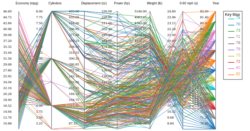
Figure 2: Caption place holder

Figure 2 presents the benchmarking results, as illustrated in the previous section, for all JSOL visualization, the time it takes starting from page loading to rendering scene graphs typically faster than most of the libraries; the main reason is the HTML5 Canvas built on top of WebGL that uses graphics card as a computational booster.

First and foremost, we have to load the data variable, CSV type in this situation (For JSON, specify the type to be ”json”). We can import from multiple data sources and execute some operation on them using transformation and statistics layers.

⬇

”data”: [{

”name”: ”crimea”,

”values”: ”crimea-parallel.csv”,

”format”: {

”type”: ”csv”

}

}]

After finishing data loading, the transformation phase begins, since we do not need it in the situation, we specify it to be empty.

⬇

”transform”: []

We then move to set scales used for the axes, in this example, we will use the linear scale as the data does not need scaling. We can use as many scales as we want. ⬇ ”scales”: { ”name”: ”xscale”, ”type”: ”linear”, ”range”: { ”type”: ”range”, ”value”: [0, 330] }, ”domain”: { ”data”: ”crimea”, ”field”: ”name” } } ⬇ ”encoding”: { ”x”: { ”field”: ”wavelength”, ”type”: ”quantitative”, ”scale”: { ”domain”: [300,450] } }, ”y”: { ”field”: ”power”, ”type”: ”quantitative” } } Defining axes follows placing scales. An axes must have some characteristics such as:

• Type: the type in the snippet below implemented uniquely for polar parallel coordinates. There are tons of axes types.

• Properties: define aesthetics of the axes; annotation sets axes’ title text, position, and color.

• Transform: sets the transformation of axes, in our case, the axes uses the power function transformation.

And as you see in comparison code snippets, the difference between JSOL  and Vega-Lite, you can see that vega-lite for each variable you define it’s scale or uses the default scale for the type(quantitative in example), but if you are using JSOL  you only need to define the scale and use it’s name to invoke it on as many variables/axes as you want, and here you can sense the power of dynamicity.

⬇

”axes”: {

”type”: ”coord_polar_parallel”,

”properties”: [{

”type”: ”y”,

”data”: ”crimea”,

”field”: ”economy-mpg”,

”orient”: ”left”,

”grid”: false,

”text”: {

”font”: ”10px␣tohma”,

”colour”: ”blue”

},

”annotation”: {

”title”: ”economy-mpg-”,

”position”:

”edge”,

”font”: ”10px␣Arial”,

”colour”: ”␣blue”

},

”transform”: {

”function”: ”pow”,

”properties”: {

”power”: 2,

”name”: ”power”

}

}]

}

The The figures above reveal the power of using JSOL, both are [15]’s parallel coordinates, but the difference as shown is that one of them is polar which is a compelling point in the library, that you can easily convert any visualization scene from cartesian to polar coordinate in a single command.

5 Conclusion

We have presented the JavaScript Open-source Library (JSOL), the grammar of graphics JavaScript library which has the power to generate the most captivating plots with no limitations. JSOL is implemented using JavaScript, which enabled it to be integrable to many other fields. We also demonstrated how it works internally by describing its layers’ specification, role, and the architectural design. We discussed how JSOL accompanies the Human-Computer Interaction (HCI) principles. Manipulating data is a crucial part of JSOL, the way data loaded from various sources, and how transformation (e.g., filtering and grouping) and statistical (e.g., mean and std) operations are applied, the way of generating scales for mapping data fed to the geometries layer proffered JSOL an edge while comparing to other libraries. Another contribution of the library is the way of combining low-level visualization layer with the compilation process. And we considered a comparative study between JSOL and great libraries such [3] and [5], and a comprehensive comparison with [6]. Finally, we explained how to use JSOL through numerous examples such as the parallel plot in Cartesian and Polar scales.

References

- [1] W. A. Yousef, H. E. Mohammed, A. A. Naguib, Y. M. Khalifa, A. M. Mamdoh, E. A. Awad, N. A. S. S. T. AbdElrheem, and S. G. Gaafar, “Jsol: Javascript-based open-source library,” 2016. [Online]. Available: https://github.com/hci-lab/JSOL
- [2] W. A. Yousef, A. A. Abouelkahire, O. S. Marzouk, S. K. Mohamed, and M. N. Alaggan, “DVP: Data Visualization Platform,” arXiv preprint arXiv:1906.11738, 2019.
- [3] M. Bostock, V. Ogievetsky, and J. Heer, “D3: Data-driven documents,” IEEE Trans. Visualization & Comp. Graphics (Proc. InfoVis), 2011. [Online]. Available: http://vis.stanford.edu/papers/d3
- [4] M. Bostock and J. Heer, “Protovis: A graphical toolkit for visualization,” IEEE transactions on visualization and computer graphics, vol. 15, no. 6, 2009.
- [5] H. Wickham, ggplot2: Elegant Graphics for Data Analysis. Springer-Verlag New York, 2009. [Online]. Available: http://ggplot2.org
- [6] A. Satyanarayan, D. Moritz, K. Wongsuphasawat, and J. Heer, “Vega-lite: a grammar of interactive graphics,” IEEE Transactions on Visualization and Computer Graphics, vol. 23, no. 1, pp. 341–350, 2017.
- [7] C. Lutz, F. Wolter, and M. Zakharyaschev, “A tableau algorithm for reasoning about concepts and similarity,” in Automated Reasoning with Analytic Tableaux and Related Methods, M. Cialdea Mayer and F. Pirri, Eds. Berlin, Heidelberg: Springer Berlin Heidelberg, 2003, pp. 134–149.
- [8] L. Wilkinson, The Grammar of Graphics (Statistics and Computing). Secaucus, NJ, USA: Springer-Verlag New York, Inc., 2005.
- [9] C. Stolte, D. Tang, and P. Hanrahan, “Polaris: a system for query, analysis, and visualization of multidimensional databases,” Commun. ACM, vol. 51, no. 11, pp. 75–84, Nov. 2008. [Online]. Available: https://doi.org/10.1145/1400214.1400234
- [10] R. E. Bellman, Adaptive Control Processes. Princeton, NJ: Princeton University Press, 1961.
- [11] D. A. Norman, The Design of Everyday Things. New York, NY, USA: Basic Books, Inc., 2002.
- [12] J. Nielsen, “Usability inspection methods,” in Conference Companion on Human Factors in Computing Systems, ser. CHI ’94. New York, NY, USA: ACM, 1994, pp. 413–414. [Online]. Available: https://doi.org/10.1145/259963.260531
- [13] L. L. Constantine and L. A. D. Lockwood, Software for Use: A Practical Guide to the Models and Methods of Usage-centered Design. New York, NY, USA: ACM Press/Addison-Wesley Publishing Co., 1999.
- [14] R. L. M. F. Molly Follette Story, James L. Mueller, The Universal Design File: Designing for People of All Ages and Abilities. Revised Edition., 1998.
- [15] A. Inselberg and B. Dimsdale, “Parallel coordinates: A tool for visualizing multi-dimensional geometry,” in Proceedings of the 1st Conference on Visualization ’90, ser. VIS ’90. Los Alamitos, CA, USA: IEEE Computer Society Press, 1990, pp. 361–378. [Online]. Available: http://dl.acm.org/citation.cfm?id=949531.949588