Instabilities, Anomalous Heating and Stochastic Acceleration of Electrons in Colliding Plasmas

Abstract

The collision of two expanding plasma clouds is investigated, emphasizing instabilities and electron energization in the plasma mixing layer. This work is directly relevant to laboratory experiments with explosively-created laser or z-pinch plasmas but may also elucidate naturally occurring plasma collisions in astrophysical or space physics contexts. In the previous publications [MalkovSotnikov2018PhPl, Sotnikov2020], we have studied, analytically and numerically, the flow emerging from interpenetrating coronas launched by two parallel wires vaporized in a vacuum chamber. The main foci of the studies have been on the general flow pattern and lower-hybrid and thin-shell instabilities that under certain conditions develop in the collision layer. The present paper centers around the initial phase of the interpenetration of the two plasmas. A two-stream ion-ion instability, efficient electron heating, and stochastic acceleration dominate plasma mixing at this phase. Both the adiabatic (reversible) electron heating and stochastic (irreversible) acceleration and heating mechanisms, powered by unstably driven electric fields, are considered. The irreversibility results from a combination of electron runaway acceleration in the wave electric fields and pitch-angle scattering on ions and neutrals.

I Introduction

Macroscopic plasma motions often harbor microscopic phenomena that are challenging to understand or even observe. The hi-speed collision of two plasma clouds is an excellent example of how microinstabilities control the macroscopic flow that results from the collision. The collision of ordinary gases results in a contact surface and a pair of shocks propagating into each gas. No mixing other than a relatively slow diffusion across the contact surface is expected, at least in a perfectly symmetric stable flow. Plasma collisions are different in several ways. First, colliding plasma clouds may go through each other without much effect. This regime is expected when the relative plasma motion is collisionless, owing to its high velocity, whereas the individual plasmas may or may not be. At the same time, instabilities associated with the relative motion (two-stream instability) may have no time to develop during the plasma interaction or be suppressed by the internal pressure of the streams [VVS_1961SvPhUsp]. The difference in collisionality regimes may occur when the relative velocity between the clouds is much larger than the thermal velocity in each of them, owing to the steep growth of the collision mean free path with the relative particle velocity, $\lambda\propto v^{4}$. Sustainable counterstreaming ion flows have also been observed in numerical simulations with a contact discontinuity-type of initial state [Moreno_2019]. The interpenetration of adjacent plasmas of different densities results in a phase space structure where mixed populations intersperse residual areas of counterstreaming protons. So the phase-space develops density holes.

This paper will consider microscopic instabilities and electron heating in interpenetrating plasmas using unmagnetized plasma approximation near a symmetry plane of collision. The collision regime of magnetized electrons and unmagnetized ions has been addressed in [MalkovSotnikov2018PhPl] along with the macroscopic two-dimensional flow emerging from the collision. Macroscopic instabilities of this flow have been studied numerically in [Sotnikov2020] in hydrodynamic approximation. When focusing on the microscopic instabilities and associated heating processes, further progress can be made by considering plasma interpenetration along the centerline in one dimension, which we pursue in this paper.

Plasma collisions are best studied in experiments with laser and z-pinch plasmas. The present work is motivated by laboratory experiments with two ohmically-exploding parallel wires. Being vaporized, they launch plasma coronas toward each other. The interpenetration and mixing of the hot coronas are followed by a collision and mixing of denser phases of the melted wire material. They are also much colder than the coronas, weakly ionized, and move at an order of magnitude lower speed (typical at 3-5 km/s vs. 50-100 km/s, [Sarkisov2005]).

Nevertheless, this phase is characterized by protracted light emission from the collision layer, which is considerably less pronounced and shorter in time in the case of a single wire explosion. The difference speaks to the importance of the corona interpenetration stage of the collision process. Otherwise, two closely spaced parallel wires would exhibit the same flow morphology as a single wire with a similar total energy deposition. On the contrary, the single- and double-wire explosions show different emission patterns in intensity and morphology. Namely, the double-wire explosion develops a thin glowing layer between the two wires. It extends symmetrically to a chamber scale, remains narrower than the gap between the wires, and persists for times until their core material engulfs the entire chamber.

Turbulent electron heating and acceleration during the early stage of corona interpenetration may enhance the line emission from the colliding neutral core materials that trail coronas. This premise and the above considerations have motivated the present study. Besides, we are interested in characterizing the entire collision in terms of its scales, growth rates, and thresholds of underlying instabilities. Spatio-temporal characteristics of the instabilities and associated turbulent motion is another objective of this study.

The analytic and numerical studies in [MalkovSotnikov2018PhPl, Sotnikov2020] have indicated that plasmas that stream against each other from two ohmically vaporized wires may indeed mix in a relatively thin layer, in accord with the preceding experiments [Sarkisov2005]. The shocked corona layer is separated from the inflowing material by a pair of termination shocks (for supersonic flows), and the plasma pressure inside the layer reaches its maximum at the flow stagnation point. The emerging pressure gradient drives two symmetric outflows perpendicular to the plane of the wires. These outflows are squeezed between the inflowing coronas of the exploded wires (see, e.g., Figs.4-9 in [Sotnikov2020]). A similar flow pattern forms a dense material of the wires that follows the corona flow (Fig.10 in the above reference). The flow pattern is qualitatively similar for the collisionless and hydrodynamic regimes. The role of pressure in the former case plays electrostatic and pondermotive potentials. The electrostatically mediated flow in the case of Boltzmannian electrons is formally equivalent to the hydrodynamic flow with an adiabatic index $\gamma=1$. This analogy justifies hydrodynamic simulations of colliding plasmas [Sotnikov2020] as a guide for studying the microscopic processes to which we turn in the present paper. Besides, the $\gamma=1$ value indicates that the shocks are radiative, which is consistent with the enhanced emission from a surprisingly thin shocked plasma layer observed in the experiments. The thin layer points to high shock compression, characteristic of radiative shocks.

The remainder of the paper is organized as follows. In the next section, we consider instabilities that we expect to develop when two coronas from exploded wires begin to penetrate each other. In Sec.II, we first evaluate the electron response to the unstable waves and obtain their velocity distribution established in the turbulent electric field of these waves in an adiabatic (non-resonant) wave-particle interaction regime. Next, in Sec.III.2, we include the electron-ion and electron-neutral collisions, thus making electron dynamics irreversible. In particular, we will obtain the steady-state analytic solutions to the problem and time-dependent, numerical ones. We conclude the paper in Sec.IV with a summary of the results and a brief discussion.

II Two-Stream Instability in Counterstreaming Plasmas

When two coronas expanding from electrically exploded wires collide supersonically, the collision region is bound by a pair of termination shocks that propagate into the inflowing plasmas on each side of the shocked layer. In both high- and low-Mach-number cases, an electrostatic potential builds up between interpenetrating coronas and slows their ions down before the mixed flow deflects off the plane of the two wires. To produce such deflection, the electrostatic potential, $\Phi$, must reach the level of

$$e\Phi\sim Mu^{2}$$

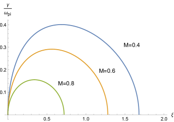
Figure 1: Growth rate of the two-stream instability as described by eq.(4).

where $u$ is the speed of plasma upstream of the collision layer, and $M$ is the ion mass. In more detail, a two-dimensional flow that emerges from the collision of two concentric outflows has been studied using the hodograph transformation in [MalkovSotnikov2018PhPl]. The magnetic field carried to the collision layer with the flows is assumed to have no substantial effect on the ion motion since the flow ram pressure is typically about an order of magnitude higher than the magnetic pressure [Sarkisov2005]. This condition is equivalent to the ion Larmor radius $\rho_{i}\sim u/\omega_{ci}$ being much larger than the ion skin depth, which is the basic scale of a magnetized collisionless shock. However, electrons are likely to be magnetized, at least before being heated, so that the electric field produces an $\boldsymbol{E}\times\boldsymbol{B}$ drift of electrons with the drift velocity:

$$V_{E}\sim c\Phi/LB$$

where $L$ is the characteristic scale of the potential $\Phi$ that slows the ions down. Therefore, the electron drift velocity $V_{E}$ can be estimated as follows:

$$V_{E}\sim\frac{\rho_{i}}{L}u.$$

The collision region, where the counterstreaming flows slow down as they approach the mid-plane, is expected to undergo the following. Initially, one of the rapidly growing electron-scale instabilities sets in, depending on the velocity of the relative motion and thermal velocities of the interpenetrating plasmas. The typical speed of the relative motion is of the order of a several $10$km/s [Sarkisov2005], whereas the electron thermal velocity is considerably higher, up to $10^{3}$km/s. The Buneman-type two-stream electron instability requires $u>V_{Te},$and probably does not start. Even if it does, it will quickly thermalize and mix up the electron populations before the much heavier ions start responding to this instability. The modified two-stream instability, in which electrons ExB drift in the wire direction, has been considered [MalkovSotnikov2018PhPl]. It should produce a similar effect of electron preheating. After the saturation of these fast instabilities, a slower instability of the counterstreaming ions will develop at their (slower) time scale. A simple dispersion relation for this instability, written down in the limit of monoenergetic counterstreaming ion beams, has the following form

$$1+\chi_{e}-\frac{\omega_{pi}^{2}}{\left(\omega-ku\right)^{2}}-\frac{\omega_{pi}^{2}}{\left(\omega+ku\right)^{2}}=0$$ (1)

The last two terms come from the counterstreaming ions, moving at the bulk speeds, $\pm u$. The electron susceptibility, $\chi_{e},$ can be taken in an adiabatic approximation form

$$\chi_{e}=\frac{2}{k^{2}\lambda_{De}^{2}},$$ (2)

which requires $\omega\ll k_{z}V_{Te}$. This requirement is consistent with the electron preheating during the early stage of collision. The electron contribution in eq.(2) to the dielectric function corresponds to their density perturbations related to that of the electrostatic potential as $n_{\text{e}}^{\prime}/n_{0}\approx e$$\phi^{\prime}/T_{\text{e}}$. The coefficient ’2’ in the above expression stands for the two electron populations that neutralize the respective ion beams of a number density $n_{0}$.

The role of the magnetic field is difficult to foresee, as it is of opposite polarity in the inflowing coronas and may undergo a significant turbulent reconnection/annihilation as the plasmas mix together. It is possible that as the two plasmas expand adiabatically before they collide, the regime of hot electrons, implied in eqs.(1) and (2), is established only after significant interpenetration and heating of the coronas. During the initial collision phase, an opposite regime of cold electrons, $k_{z}V_{Te}\ll\omega$, is more likely to occur. Assuming that the unstable waves have a small wave vector component along the magnetic field at this stage, $\chi_{e}$ takes a different form. Indeed, if the electrons are magnetized in their motion across the local magnetic field, $\omega_{ci}\ll\omega\ll\omega_{ce}$, instead of eq.(2) we can write

$$\chi_{e}=2\frac{\omega_{pe}^{2}}{\omega_{ce}^{2}}-2\frac{k_{z}^{2}}{k^{2}}\frac{\omega_{pe}^{2}}{\omega^{2}}$$ (3)

The significance of this form of $\chi_{e}$ is a lower instability threshold for certain wavenumbers. In this case, however, the instability saturates more easily by electron heating. We will therefore override the phase of initial electron heating and return to the adiabatic regime, which we justify below. But, first, let us introduce the following dimensionless parameters:

$$\xi=\frac{k^{2}u^{2}}{\omega_{pi}^{2}},\,\,\,\,\,\,\,\,\,\,\mathcal{M}^{2}=\frac{u^{2}}{C_{s}^{2}}\equiv M\frac{u^{2}}{T_{e}}.$$

Using this notation, eq.(1) rewrites

$$1+\frac{2\mathcal{M}^{2}}{\xi}-\frac{1}{\left(\Omega-\sqrt{\xi}\right)^{2}}-\frac{1}{\left(\Omega+\sqrt{\xi}\right)^{2}}=0.$$

One of its solutions describes an aperiodically growing mode, Fig.1:

$$\frac{\omega^{2}}{\omega_{pi}^{2}}\equiv\Omega^{2}=-\frac{\xi}{\xi+2\mathcal{M}^{2}}\left(\sqrt{8\mathcal{M}^{2}+4\xi+1}-1-2\mathcal{M}^{2}-\xi\right)$$ (4)

The aperiodic instability ($\omega^{2}<0$) develops when the term in parentheses in eq.(4) is positive. The condition for that can be written in the following short form:

$$\mathcal{M}^{2}+\frac{\xi}{2}<1$$ (5)

We observe that this condition can be met only in subsonic flows. Such flows are expected in the plasma collision region, even if the flows are initially highly supersonic, such as $u\gtrsim V_{Te}$. In this case, as we discussed, the electrons should be heated via Buneman instability. Likewise, the interpenetrating flows will also be subsonic when standing termination shocks are formed on the two sides of the collision zone. We should note here, though, that a situation in which the flows are supersonic but not to the extent sufficient for triggering the Buneman instability is also possible. In this case, electrons can be preheated by other instabilities, such as the modified two-stream instability, leading to the generation of lower-hybrid waves. This case has already been considered in Ref.MalkovSotnikov2018PhPl. We may conclude from the above considerations that at least one of the discussed instabilities will result in electron preheating. We will, therefore, continue our analysis of a slower, two-stream ion instability under the assumption $\omega\ll k_{z}V_{Te}$.

The above ion-driven instability can be suppressed if ions in the beam are also heated by generated waves or arrive in the collision zone with a significant velocity dispersion, carried over from the wire evaporation. We assume the finite ion thermal speed in each ion beam, $V_{Ti}$, to examine this possibility. Eq.(1) generalizes to the following [VVS_1961Usp] (see Appendix)

$$1+\frac{2}{k^{2}\lambda_{De}^{2}}-\frac{\omega_{pi}^{2}}{\left(\omega-ku\right)^{2}-k^{2}V_{Ti}^{2}}-\frac{\omega_{pi}^{2}}{\left(\omega+ku\right)^{2}-k^{2}V_{Ti}^{2}}=0$$ (6)

Again, coefficient 2 in the electron contribution accounts for the two electron components that neutralize the two counterstreaming ion beams. These are represented by the last two terms on the l.h.s. of the above equation. Using the dimensionless variables introduced earlier, we rewrite this equation as follows

$$1+\frac{2}{k^{2}\lambda_{De}^{2}}-\frac{1}{\left(\Omega-\sqrt{\xi}\right)^{2}-k^{2}\lambda_{Di}^{2}}-\frac{1}{\left(\Omega+\sqrt{\xi}\right)^{2}-k^{2}\lambda_{Di}^{2}}=0$$ (7)

A compact expression for the solution can be obtained using the parameters $\mathcal{M}$ and $\zeta\equiv 2+\xi/\mathcal{M}^{2}$:

$$\Omega^{2}\equiv\frac{\omega^{2}}{\omega_{pi}^{2}}=\left(\zeta-2\right)\left[\mathcal{M}^{2}+\frac{1}{\zeta}+\frac{T_{i}}{T_{e}}-\frac{1}{\zeta}\sqrt{4\zeta\mathcal{M}^{2}\left(1+\frac{T_{i}}{T_{e}}\zeta\right)+1}\right]$$ (8)

For the onset of instability, the r.h.s of this expression should be negative. This condition can be manipulated into the following inequality

$$0<\zeta\left(\mathcal{M}^{2}-\frac{T_{i}}{T_{e}}\right)<2,$$

which, in turn, can be rewritten as the following constraint on the Mach number of the counterstreaming flows:

$$\frac{T_{i}}{T_{e}}<\mathcal{M}^{2}<\frac{T_{i}}{T_{e}}+\frac{1}{1+k^{2}C_{s}^{2}/2\omega_{pi}^{2}},$$

or on their velocity:

$$\frac{T_{i}}{M}<u^{2}<\frac{T_{i}}{M}+\frac{C_{s}^{2}}{1+k^{2}C_{s}^{2}/2\omega_{pi}^{2}}.$$ (9)

The growth rate given in eq.(2) is shown in Fig.2 as a function of $\xi$ and $T_{i}/T_{e}$ for $\mathcal{M}=0.4$. The instability obviously, disfavors short waves, for which even insignificant change of ion temperature or the flow velocity $u$, or both, may produce a stabilizing effect. The electron heating, on the contrary, widens the range of the flow velocities where the instability may develop. Under these circumstances, it seems plausible to investigate electron heating in more detail. Due to the low mass ratio, electrons will be heated more efficiently than ions as the instability develops. Electron heating broadens the velocity range of unstable modes and impedes their stabilization, based on the above criterion.

III Electron Heating and Acceleration

At least in a linear approximation, the instability considered above excites electrostatic perturbations that are non-propagating in the laboratory frame. Physically, the instability may be thought of as intersecting backward-propagating ion-acoustic modes in each of the two plasmas. They have phase velocities $\left|\omega_{\pm}/k\right|=u$, where $\omega_{\pm}$ denote the wave frequencies in the frames of the two counterstreaming plasmas. They resonate with each other in the laboratory frame, in which they do not propagate. So, the mode grows aperiodically.

III.1 Rapid Electron Preheating

The counterstreaming ion instability discussed in the previous section has a growth rate $\gamma_{k}<\omega_{\text{pi}}$, so the electrons respond adiabatically, as we assumed in deriving the dispersion relation, that is $kV_{\text{Te}}\sim\omega_{\text{pi}}V_{\text{Te}}/u>\gamma_{k}$. Representing then the fluctuating electric field as a superposition of growing modes, $E=\sum_{k}E_{k}\left(t\right)\exp\left(i\boldsymbol{kr}\right)$, we can write the following quasilinear equation for the heating process, e.g., [SagdGal69]

$$\frac{\partial f_{e}}{\partial t}=\frac{e^{2}}{m^{2}}\frac{\partial}{\partial\boldsymbol{v}}\sum_{k}\frac{\gamma_{k}\left|E_{k}\right|^{2}}{k^{2}v^{2}+\gamma_{k}^{2}}\frac{\partial f_{e}}{\partial\boldsymbol{v}}$$ (10)

This equation describes nonresonant interaction of electrons with the unstable waves. Based on our assumption of electron adiabaticity, $kV_{Te}>\gamma_{k}$, we can neglect the $\gamma_{k}^{2}$ in the denominator of the above expression. Next, we introduce the electron velocity diffusion coefficient and represent it in the form

$$D_{e}=\frac{e^{2}}{2m^{2}}\frac{\partial}{\partial t}\sum_{k}\left|\phi_{k}\right|^{2}=\frac{e^{2}}{m^{2}}\sum_{k}\gamma_{k}\left|\phi_{k}\right|^{2},$$

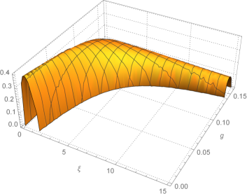
Figure 2: Instability growth rate given by eq.(8) for $\mathcal{M}=0.4$ as a function of $\xi$ and $g\equiv T_{i}/T_{e}$.

where we have denoted the spectral components of the wave electric potential by $\left|\phi_{k}\right|=\left|E_{k}/k\right|$. Introducing then a new variable

$$\tau=\frac{e^{2}}{2m^{2}}\sum_{k}\left|\phi_{k}\left(t\right)\right|^{2},$$

instead of $t$ and assuming first a one-dimensional spectrum of electrostatic perturbations oriented along the flow, eq.(10) can be written in the following short form

$$\frac{\partial f_{e}}{\partial\tau}=\frac{\partial}{\partial v}\frac{1}{v^{2}}\frac{\partial f_{e}}{\partial v}$$

The last equation has a simple self-similar solution:

$$f_{e}=\frac{C}{\tau^{1/4}}\exp\left(-\frac{v^{4}}{16\tau}\right)$$

where C is a normalization constant. This solution describes reversible electron heating that disappears together with the field oscillations. The perceived electron “temperature”, $T_{e}^{\text{*}}=2\sqrt{\tau}$, in the above formula merely reflects the amplitude of coherent electron oscillations in an ensemble of waves with random phases.

In the case of three-dimensional isotropic fluctuations, the above equation takes a slightly different form

$$\frac{\partial f_{e}}{\partial\tau}=\frac{1}{v^{2}}\frac{\partial^{2}f_{e}}{\partial v^{2}}$$

but its solution has a similar dependence on the particle velocity:

$$f_{e}=\frac{C}{\tau^{3/4}}\exp\left(-\frac{v^{4}}{4\tau}\right),$$

as well as the same physical meaning as in the one-dimensional case.

While the adiabatic heating of electrons may impart significant amount of kinetic energy, the energized electrons will cool down as soon as the oscillations are damped or disappear otherwise, e.g., propagate away from the excitation region. On the other hand, it is not difficult to imagine a situation in which the entropy of electron gas increases, thus rendering the heating process irreversible with no substantial energy input. It might come about in two different ways or as a combination thereof. In one way, the random but fixed phases of the waves begin to evolve dynamically with a certain degree of stochasticity, which should randomize the electron trajectories. In a second way, the electron orbits are randomized independently of the oscillating field that sets them in motion. Such a randomizing factor can be the scattering of electrons on ions and neutrals in the shocked plasma layer. Since we expect such scattering in the mixing layer, we include it in the electron kinetics below, which will make the adiabatic heating irreversible.

III.2 Stochastic Heating and Runaway Acceleration of Electrons in The Shocked Plasma Layer

Observations of enhanced emission near the flow stagnation region in experiments, e.g., [Sarkisov2005], suggest that the shocked plasma thermalizes most rapidly where the counterstreaming flows collide head-on. Due to their rapid response to the instability, considered earlier, the two counterstreaming electron distributions will couple and form essentially one distribution with a zero average drift speed across the layer. At the same time, ions will continue counterstreaming, thus providing free energy for the instability considered in the preceding section. The instability should, however, eventually saturate. The most straightforward saturation mechanism is the convection of electrostatic perturbations with plasma outflow from the instability region in the layer direction.

Meanwhile, the merger of electron distributions cannot be completed everywhere in the mixing layer, especially at its edges. s. Therefore, we first describe electrons that inflow into the mixing region from its opposite sides as separate components and denote their distributions as $f_{\pm}$, so that the full electron distribution is simply $f=f_{\text{+}}+f_{-}$. The distributions $f_{\pm}$ enter the collision layer with drift velocities $\pm u$, respectively. The equations for $f_{\pm}$ can be written as follows

$$\frac{\partial f_{\pm}}{\partial t}+\left(v\mu\pm u\right)\frac{\partial f_{\pm}}{\partial z}-\frac{e}{m}E\left(\mu\frac{\partial f_{\pm}}{\partial v}+\frac{1-\mu^{2}}{v}\frac{\partial f_{\pm}}{\partial\mu}\right)=\frac{1}{v^{2}}\frac{\partial}{\partial v}\left[v^{2}\nu_{\text{e}}\left(V_{\text{Te}}^{2}\frac{\partial f_{\pm}}{\partial v}+vf_{\pm}\right)\right]+\frac{\nu}{2}\frac{\partial}{\partial\mu}\left(1-\mu^{2}\right)\frac{\partial f_{\pm}}{\partial\mu}$$ (11)

where we have denoted

$$\nu_{\text{e,i}}=\frac{4\pi e^{4}N_{\text{e,i}}}{m^{2}v^{3}}\ln\left(\frac{mv^{2}\lambda_{\text{De}}}{e^{2}}\right)$$ (12)

and

$$\nu=\nu_{\text{i}}+\nu_{\text{e}}\left(1-\frac{V_{\text{Te}}^{2}}{v^{2}}\right)$$ (13)

Below, explain the two equations for $f_{\pm}$ combined in eq.(11) for simplicity. Formally, they are written in separate reference frames moving with velocities $\pm u$ in $z-$direction, so that the velocity projection on $z$ direction is $v\mu\pm u$ in each of these equations. The cosine of the particle pitch-angle to the shock normal ($z$- direction), $\mu$, is introduced in a standard form $v_{z}=v\mu$, where $v_{z}$ is the $z-$ component of electron velocity $\boldsymbol{v}$. Apart from the terms with $\pm u$ on the lhs of eqs.(11), the equations for $f_{\pm}$ are identical. Moreover, since $v$ is at least $v\sim V_{\text{Te}}\gg V_{\text{Ti}}\sim u$, or even $v\gg V_{\text{Te}}$, since we expect significant electron heating and acceleration by turbulent electric field, $E$, we assume that $f_{\text{+}}\approx f_{-}$ inside the shocked layer. The role of the $\pm u$ term is then limited to the edges of the layer where initially cold electrons enter the layer from opposite sides. Likewise, the pitch-angle scattering operator (the last term on the rhs) can be regarded as acting in the laboratory rather than separately in each of the comoving reference frames, as originally required in eq.(11). Except for $z-$dependence (introduced straightforwardly), separation of the two groups of electrons $f_{\pm}$, and an oscillatory rather than the constant electric field, $E$, eq.(11) is similar to that used in studies of electron runaway, e.g., [Gurevich61RunAway, KruskalBernstein64].

III.2.1 Equation for runaway electrons

Taking the above discussion into account, introducing pitch-angle averaged quantities

$$\left\langle\cdot\right\rangle=\frac{1}{2}\int_{-1}^{1}\left(\cdot\right)d\mu,$$

and averaging eq.(11) over $\mu$, we arrive at the following equation for $f=f_{\text{+}}+f_{-}$:

$$\frac{\partial\left\langle f\right\rangle}{\partial t}+\frac{1}{2}\left(\frac{eE}{mv^{2}}\frac{\partial}{\partial v}v^{2}-v\frac{\partial}{\partial z}\right)\left\langle\left(1-\mu^{2}\right)\frac{\partial f}{\partial\mu}\right\rangle=\frac{1}{v^{2}}\frac{\partial}{\partial v}\left[v^{2}\nu_{\text{e}}\left(V_{\text{Te}}^{2}\frac{\partial\left\langle f\right\rangle}{\partial v}+v\left\langle f\right\rangle\right)\right]+\left\langle S\right\rangle$$ (14)

Here the term $\left\langle S\right\rangle$ arose from summing up the fluxes $\pm uf_{\pm}$ through the boundaries of the layer. They are not accounted for automatically when we add the equations for $f_{\pm}$ together in eq.(11) and assume $f_{\text{+}}=f_{-}$. The reason for this extra term is that $f_{\text{+}}$$\neq f_{-}$ near the boundaries, which we mentioned earlier. We may include in the term $\left\langle S\right\rangle$ other transport channels, such as particle convection along $x$ and y axes. To obtain an evolution equation for $\left\langle f\right\rangle$, we need to express the $\left\langle\left(1-\mu^{2}\right)\partial f/\partial\mu\right\rangle$ in the last equation through $\left\langle f\right\rangle$. This can be done by applying Chapman-Enskog method to eq.(11). This method will provide an expansion of equation for $\left\langle f\right\rangle$ in powers of $\overline{E^{2}}$- an average value of $E^{2}$ over the distance and time that exceeds the mfp $\lambda=v/\nu$ and collision time $1/\nu$, respectively. In particular, if the electric field comes from the instability of counterstreaming ion beams considered earlier, $E=\left(1/\sqrt{2}\right)\sum_{k}E_{k}\left(t\right)\exp\left(ikz\right)+c.c.$, then $\overline{E^{2}}=\sum_{k}\left|E_{k}\right|^{2}$.

The Chapman-Enskog method selects the zeroth order approximation that makes the rhs (particle collision part) vanish. This is the assumption for a system being close to thermal equilibrium. However, the collision operator on the rhs of eq.(11) acts on the angular part and the absolute value of particle velocity separately. Now we consider the second term (angular part) on the rhs of eq.(11) to be dominant. Although it is formally of the same order as the first term, it must vanish in the zeroth order by virtue of eq.(14), as we can set $\left\langle S\right\rangle\approx 0$ inside the shocked plasma, as discussed earlier. Also note that for a Maxwellian distribution, $f\propto\exp\left(-v^{2}/V_{\text{Te}}^{2}\right)$, the collision term vanishes. As we shall see, for higher velocities the runaway due the secular action of electric field dominates the thermal equilibtration represented by the rhs in eq.(14). This dominance justifies neglecting the first term on the rhs of eq.(11) for the purpose of calculation of anisotropic correction to the equilibrium state.

Turning to the lhs of eq.(11) we note that the first term ($\partial f/\partial t$) needs to be dropped to this order of approximation as it is responsible for a short-time relaxation of the anisotropic component, e.g. [MS2015]. From eq.(11), to the first order, we thus write

$$\frac{\partial f}{\partial\mu}\approx\frac{1}{\nu}\left(\frac{eE}{m}\frac{\partial\left\langle f\right\rangle}{\partial v}-v\frac{\partial\left\langle f\right\rangle}{\partial z}\right)$$

On substituting this expression into eq.(14), the latter takes the following form

$$\frac{\partial\left\langle f\right\rangle}{\partial t}=\frac{1}{v^{2}}\frac{\partial}{\partial v}v^{2}\left[\left(\nu_{\text{e}}V_{\text{Te}}^{2}+\frac{e^{2}\overline{E^{2}}}{3m^{2}\nu}\right)\frac{\partial\left\langle f\right\rangle}{\partial v}+\nu_{\text{e}}v\left\langle f\right\rangle\right]+\left\langle S\right\rangle+\frac{v^{2}}{3\nu}\frac{\partial^{2}\left\langle f\right\rangle}{\partial z^{2}}$$ (15)

The last term on the rhs governs the diffusive losses from the shocked layer. They might extend to the other coordinates, which can symbolically be included into the $\left\langle S\right\rangle$-term, as we mentioned earlier. The losses become important for large $v$, where they equate the acceleration $\propto\overline{E^{2}}$. The acceleration occurs in the plasma mixing layer that is bound by a pair of termination shocks at $z=\pm l/2$. A plausible assumption about the distribution of accelerated electrons in $z$- direction is that their density vanishes at $z=\pm l/2$. The reason for this assumption is twofold. First, the shocked layer has an elevated electrostatic potential that slows down the inflowing ions in $z$ direction. Hence, this region is a potential well for electrons, so they tend to have a higher concentration toward the middle of this region. Second, the high-energy electrons, for which the losses become significant, most likely never return to the shocked layer if they cross one of its edges. Indeed, the flow upstream of the termination shocks is relatively laminar. This means that hot electrons accelerated in the mixing layer by the turbulent electric field are not deflected strongly from their paths. Their transport regime changes at the edge from diffusive to ballistic. Depending on the electron energy and magnetic field strength, electrons leave the layer by either following rectilinear trajectories or by ExB drifting away from the flow stagnation region across the magnetic field convected with the upstream flow. Therefore, we may use the following expansion for $\left\langle f\right\rangle$ in $z$- direction

$$\left\langle f\right\rangle=\sum_{n=1}^{\infty}f_{n}\left(t,v\right)\cos\left(\frac{\pi nz}{l}\right)$$ (16)

While this representation implies instantaneous losses of hot electrons from the shocked layer as soon as they reach its boundaries at $z=\pm l/2$, there is also an influx of cold electrons from the upstream. By keeping only the leading term in the last Fourier expansion, eq.(15) can be rewritten as follows

$$\frac{\partial f_{1}}{\partial t}=\frac{1}{v^{2}}\frac{\partial}{\partial v}v^{2}\left[\left(\nu_{\text{e}}V_{\text{Te}}^{2}+\frac{e^{2}\overline{E^{2}}}{3m^{2}\nu}\right)\frac{\partial f_{1}}{\partial v}+\nu_{\text{e}}vf_{1}\right]+S_{1}-\frac{\pi^{2}v^{2}}{3l^{2}\nu}f_{1}$$ (17)

Here, we have included the input of the $\left\langle S\left(z\right)\right\rangle$-term in eq.(15) and denoted it by $S_{1}$. Note that both $V_{\text{Te}}$ and $\overline{E^{2}}$ in the last equation, generally speaking, depend on time. We start, however, from considering a steady state solution of the above equation, assuming that these quantities have already attained their time-asymptotic magnitudes.

III.2.2 Steady State Fermi acceleration of Runaway Electrons

Since the source term $S_{1}$ in eq.(17) is associated with the influx of relatively cold electrons into the shocked plasma layer, it is plausible to place it at the origin in the velocity space. Thus, we set $S_{1}=S\delta\left(v\right)/v^{2}$. Then, a steady state solution for $v>0$ corresponds to a constant electron flux $S$ between the source and the sink (the last term in eq.[17] controls the particle losses) in velocity space:

$$S=-v^{2}\left[\left(\nu_{\text{e}}V_{\text{Te}}^{2}+\frac{e^{2}\overline{E^{2}}}{3m^{2}\nu}\right)\frac{\partial\left\langle f\right\rangle}{\partial v}+\nu_{\text{e}}v\left\langle f\right\rangle\right]=cosnt$$ (18)

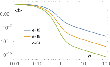
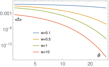
Figure 3: Left panel: steady state solutions of eq.(21) plotted for different $\vartheta$. To emphasize the development of the runaway tail, the normalization constant $\sigma$ in each curve is chosen to satisfy the condition $\left\langle f\left(0\right)\right\rangle=1$, for all $\vartheta$ rather than fixing the total number of particles. Right panel: the same solution shown as a function of $\vartheta$ for different particle energies, $w$.

This spectrum will cut off at sufficiently large $v$ due to losses, which we have neglected for now because they grow very sharply at high velocities (see eq.(13)) and are thus not important in the velocity range considered. For relatively low values of $\overline{E^{2}}$ and not very large $v$ (for which $\nu$ and $\nu_{\text{e}}$ would become small), the term with $E^{2}$ can be neglected and the solution for $\left\langle f\right\rangle$ is close to a Maxwellian (because $S=0$ as well for $v>0$). The electron runaway effect of the electric field becomes important for $v\gg V_{\text{Te}}$, and we can substitute $\nu\approx 2\nu_{e}$ in eq.(13). Furthermore, the expression under the logarithm in eq.(12) is typically so large that the velocity variation under the logarithm can be neglected, and $v$ can be set to a value $V_{\text{*}}$ at which the acceleration and dynamical friction terms in eq.(17) equate, that is

$$\frac{4\pi e^{4}N_{\text{e,i}}}{m^{2}v^{2}}\ln\left(\frac{mV_{\text{*}}^{2}\lambda_{\text{De}}}{e^{2}}\right)\sim\frac{e\sqrt{\overline{E^{2}}}}{m}$$

By defining then the Dreicer’s field, familiar from the theory of runaway electrons [Gurevich61RunAway, KruskalBernstein64] as

$$E_{\text{D}}=\frac{4\pi e^{3}N_{\text{e,i}}}{T_{\text{e}}}\ln\left(\frac{mV_{\text{*}}^{2}\lambda_{\text{De}}}{e^{2}}\right),$$

the critical velocity $V_{\text{*}}$ above which the runaway process dominates dynamical friction can be expressed through $E_{\text{D}}$ as follows:

$$V_{\text{*}}=V_{\text{Te}}\frac{E_{\text{D}}^{1/2}}{\left(\overline{E^{2}}\right)^{1/4}}$$ (19)

It is now convenient to use dimensionless electron energy $w=v^{2}/6^{1/3}V_{\text{Te}}^{2/3}V_{\text{*}}^{4/3}$ and field strength parameter

$$\vartheta=6^{1/3}V_{\text{*}}^{4/3}/2V_{\text{Te}}^{4/3}.$$ (20)

Using these quantities, eq.(18) can be rewritten as follows

$$\left(1+w^{3}\right)\frac{\partial\left\langle f\right\rangle}{\partial w}+\vartheta\left\langle f\right\rangle=-S\vartheta\frac{m^{2}}{eT_{\text{e}}E_{\text{D}}}\equiv-\sigma$$ (21)

This equation can be solved in quadratures:

$$\left\langle f\right\rangle=\sigma\exp\left[-\frac{\vartheta}{\sqrt{3}}\tan^{-1}\left(\frac{2w-1}{\sqrt{3}}\right)\right]\frac{\left(1-w+w^{2}\right)^{\vartheta/6}}{\left(1+w\right)^{\vartheta/3}}\int_{w}^{\infty}\frac{\left(1+w\right)^{\vartheta/3-1}dw}{\left(1-w+w^{2}\right)^{\vartheta/6+1}}\exp\left[\frac{\vartheta}{\sqrt{3}}\tan^{-1}\left(\frac{2w-1}{\sqrt{3}}\right)\right]$$ (22)

Fig.3 (left panel) shows the above solution for different values of field-strength parameter $\vartheta$. It is seen that for strong electric fields, $\vartheta\sim 1$, the power-law tail, $\left\langle f\right\rangle\propto w^{-2}\propto v^{-4}$, grows immediately from the thermal velocity. For weak fields ($\vartheta\gg 1)$ the Maxwellian core is distinct from the power-law tail of runaway electrons. On the right panel of Fig.3, the electron distribution function $\left\langle f\right\rangle$ is shown as a function of $\vartheta$ for several values of the fixed electron energies.

The asymptotic power-law energy spectrum $\left\langle f\right\rangle\propto w^{-2}$ may be interpreted as a classical Fermi acceleration at work. Fermi [Fermi49] showed that under competing particle acceleration-loss events, a power-law energy spectrum, $w^{-q}$, is naturally established. Its index $q$, which is in our case, $q=2$, is determined by the ratio of particle confinement time, $\tau_{\text{loss}}$, and its acceleration time, $\tau_{\text{acc}}$. Fermi originally devised this mechanism for galactic cosmic rays, in which case $\tau_{\text{loss}}$ is an average time spent by a CR particle in the galaxy before it escapes into the intergalactic space. The acceleration time, in turn, is simply the energy e-folding time, $dE/dt=E/\tau_{\text{acc}}$, where $E$ the particle energy. According to Fermi, the power-law index, $q$, in the particle distribution, $f\propto E^{-q}$, can be calculated as follows:

$$q=1+\frac{\tau_{\text{acc}}}{\tau_{\text{loss}}}$$

The Fermi acceleration has been recognized later as a general mechanism pertinent to many other systems where a nonthermal spectrum emerges from the balance between the particle energy gain and its loss or particle escape. In our case, accelerated particles loose energy as they scatter on slowly moving particles (thermal electrons, ions, and neutrals). Between each scattering they gain energy from the electric field. So, the energy gain and loss occur during the same time interval, $\tau_{\text{loss}}=\tau_{\text{acc}}$. The result $q=2$ immediately follows from the Fermi’s celebrated formula.

The asymptotic $q=2$ acceleration regime is pertinent to high-energy particles, for which the contribution of thermal core into the flux $S=const$ in eq.(18) can be neglected (all terms other than the acceleration term, $\propto\overline{E^{2}}$). The acceleration term, however, includes both the actual energy gain between two consecutive collisions and the particle scattering that results from these collisions. This conclusion can be inferred from the derivation of eq.(17) in Sec.III.2.1. The full steady state solution in eq.(22) does include the thermal core part of the spectrum and it has a somewhat complex form. For the high-energy particles, the asymptotic spectrum can be most easily obtained from the relation $w^{3}\partial\left\langle f\right\rangle/\partial w=-\sigma=const$, according to the insignificant role of the thermal core for particles with $w\gg 1$.

III.2.3 Time-dependent runaway

It is convenient to study time-dependent solutions of eq.(17) using a new variable $U$ instead of the particle energy $w$ or velocity $v$. These variables are related in the following way:

$$U=w^{3/2}=\frac{v^{3}}{\sqrt{6}V_{\text{Te}}V_{\text{*}}^{2}}.$$

By measuring time $t$ in the units of electron acceleration time, $\tau_{\text{a}}$ ($t/\tau_{\text{a}}\to t$), and introducing the particle loss parameter, $\lambda$, owing to their diffusion in $z-$ direction,

$$\tau_{\text{a}}^{-1}=6^{1/6}\frac{e}{m}E_{D}\frac{V_{\text{Te}}^{7/3}}{V_{\text{*}}^{10/3}},\;\;\;\;\;\lambda=\frac{3^{4/3}m^{2}}{4E_{D}^{2}e^{2}}\frac{V_{\text{*}}^{20/3}}{l^{2}V_{Te}^{8/3}}$$

eq.(17) rewrites as follows

$$\frac{\partial f_{1}}{\partial t}=\frac{\partial}{\partial U}\left[\frac{3}{2}U^{1/3}\left(1+U^{2}\right)\frac{\partial f_{1}}{\partial U}+\vartheta f_{1}\right]+\tau_{a}S_{1}-\lambda U^{5/3}f_{1}$$ (23)

This equation contains two parameters, $\vartheta$ and $\lambda$; these are the rates of collisional energy losses of runaway electrons and their escape through the boundaries of the mixing layer, respectively. Besides, the parameter $\vartheta$ determines the thermal core temperature that establishes through a balance between dynamical friction (term proportional to $\vartheta$) and velocity diffusion (term proportional to $1+U^{2}$, where the first term in the sum corresponds to the thermal velocity diffusion due to Column collisions, while $U^{2}$ stands for the anomalous velocity diffusion). The part of the velocity diffusion $\propto U^{2}$ stems from the electric field generated by the ion beam instability discussed in Sec.II.

According to our discussion in the preceding section, the source supplies particles at lower energies, that is at $U\ll 1$. To keep the treatment simple, we therefore draw equivalence between the source term and the boundary condition at the lower end of the integration domain. In other words, instead of specifying the source profile $S_{1}\left(U\right),$ we keep the value $f\left(U_{\text{min}}\right)$ fixed as a boundary condition. It is clear that acceleration is negligible near this end as long as $U_{\text{min}}\ll 1$. Also, to circumvent an insignificant problem with the algebraic singularity, $U^{1/3}$, at $U=0$ in the above equation, we set $U_{\text{min }}=0.1$ instead of $U_{\text{min }}=0$. This simplification is justified by the upper end of the integration interval being at $U_{\text{max}}\gg 1$. We then impose $f_{1}\left(U_{\text{min}}\right)=1$ and $f_{1}\left(U_{\text{max}}\right)=0$ as a complete set of boundary conditions for eq.(23). The latter condition implies that particles accelerated to $U_{\text{max}}$ escape the mixing layer regardless of the value of $\lambda$, but the effect of finite $\lambda$ is still present in the solution.

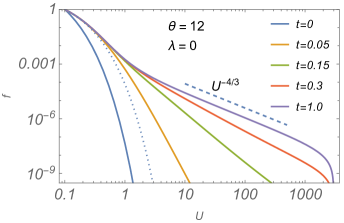
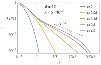
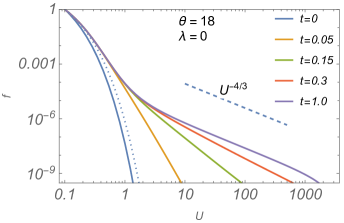
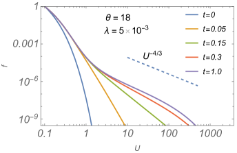
Figure 4: Time evolution of the spectrum of runaway electrons, as described by eq.(23), starting from a relatively cold initial distribution with $U_{\text{th}}=0.01$. Four combinations of equation parameters $\vartheta$ and $\lambda$ are shown in each plot. The left two panels show the loss-free solutions, $\lambda=0$, except for a particle instantaneous escape upon reaching the maximum energy at $U_{\text{max}}.$

Fig.4 illustrates the electron runaway acceleration, as it evolves in time, shown for four combinations of parameters $\vartheta$ and $\lambda$. All four runs start from a relatively cold Maxwellian (if expressed in terms of particle velocity rather than $U$):

$$f_{1}(0,U)=\exp\left[-\frac{U^{2/3}-U_{\text{min}}^{2/3}}{U_{\text{th}}^{2/3}}\right]$$ (24)

where $U_{\text{th }}$ characterizes the initial electron temperature. Although the electron adiabatic preheating, as described in Sec.III.1, should result in a steeper decay of electron distribution, we assume the above Maxwellian form. The reason for that choice is twofold. First, the initial distribution is too narrow to significantly affect its evolution beyond a short initial phase. Second, the collisional relaxation of any initial distribution localized at $U\ll 1$ dominates the evolution of $f_{1}\left(t,U\right)$ at early times. It quickly relaxes to $f_{1}\propto\exp\left(-\vartheta U^{2/3}\right)$, as can be seen from eq.(23). This initial dynamics is seen in the two left panels of Fig.4. Indeed, for the chosen two values of dynamical friction parameter, $\vartheta=12$ and $\vartheta=18$, the electron distribution broadens to the respective Maxwellian, $\exp\left(-\vartheta U^{2/3}\right)$ at $U\lesssim 1$ very quickly and proceeds then to higher energies. At $U\gtrsim 1$, the particle distribution develops a suprathermal tail that also very quickly “forgets” the initial velocity distribution.

While the initial distribution of electrons is not significant for the development of the suprathermal tail, the tail amplitude is very sensitive to the dynamical friction parameter, $\vartheta$ (see also Fig.3). As seen from Fig.4, for a 50% increase in $\vartheta$ from the top panel to the bottom ones, the tail height drops by about two orders of magnitude. This is similar to the conventional runaway process (in a constant electric field) as the suprathermal tail is detached from the thermal Maxwellian at a critical velocity, $V_{\text{*}}$, which in our case is defined in eq.(19) and is related to the dynamical friction, $\vartheta$. Because of the exponential decay of Maxwellian distribution at $v\sim V_{\text{*}}$, small variations of $V_{\text{*}}$ result in large changes in the tail height, connected to the Maxwellian at $v\approx V_{\text{*}}$.

IV Conclusions and Discussion

In this paper, we have studied microscopic processes occurring in a mixing layer between two colliding plasma clouds. Our major findings are as follows:

1. Initial relative velocity of interpenetrating plasmas needs to be in the range between the ion thermal velocity, $V_{\text{Ti}}=\sqrt{T_{\text{i}}/M}$, and ion-sound velocity, $C_{\text{s}}=\sqrt{T_{\text{e}}/M}$, for triggering a strong anomalous coupling of the plasma streams that is supported by the two-stream instability.

2. Subsequent nonresonant (reversible) heating of electrons then broadens the range of unstable wavenumbers.

3. Inclusion of electron-ion and electron-neutral collisions makes the electron energization irreversible.

4. In addition to the heating of an electron core distribution, a suprathermal power-law tail is produced in wave-particle interactions. It decays with energy as $w^{-2}$, thus showing a notable analogy with the stochastic Fermi acceleration.

5. The amplitude of the power-law electron tail strongly depends on the ratio of the turbulent electric field to the electron collision frequency.

While the instability condition in (1) may appear to be restrictive, the following arguments can be advanced in its favor. Since each of the colliding plasmas undergoes a transition from supersonic to subsonic speed in the collision region, the instability condition is likely to be met at least in a limited part of the collision region. The subsequent electron heating will then broaden the unstable range of relative velocity.

Under favorable instability conditions, specified above and in more detail in Sec.II, a significant fraction of kinetic energy of counterstreaming corona ions is likely to be converted in ion-acoustic waves. When also the electron-ion and electron-neutral collision frequencies are limited by the condition $\vartheta=6^{1/3}V_{\text{*}}^{4/3}/2V_{\text{Te}}^{4/3}\lesssim 10$ (here $V_{\text{*}}$, eq.[19], is a critical electron velocity beyond which they enter a runaway regime), the wave energy is efficiently transferred to thermal and nonthermal electrons. The anomalous (wave-driven) electron heating and acceleration will likely to have a defining impact on the next phase of plasma mixing.

The next phase starts when heavier wire-core materials, which follow the light corona plasmas, begin to interpenetrate. As the materials are largely in a neutral or weakly ionized state at the moment of touching each other, the presence of hot and suprathermal coronal electrons in the mixing layer will affect the interpenetration process by primarily ionizing the neutrals and producing line emission. Although this phase of the plasma collision was out of the scope of this paper, focused on the coronal phase, it is worthwhile to briefly discuss possible scenarios that may be derived from the presence of hot and suprathermal electrons.

As we mentioned, energetic electrons will ionize counterstreaming wire-core atoms, thus partially converting them into counterstreaming ion beams. The plasma stability analysis then becomes similar to that of the coronal collision studied earlier. However, several differences are evident. First, the beams will likely become multi-charged as the ionization potential of wire material (e.g., aluminum, tungsten) grows significantly with the charge number. Second, as the energetic electron population left behind after the coronal phase of plasma collision has a much lower concentration than the wire-core atoms, the ionization is likely to occur in an avalanche regime [GurevichUFN2001]. The neutral gas electric breakdown supported by the oscillatory electric field generated by the two-stream instability of freshly ionized beams may then naturally explain the protracted line emission observed in experiments with double-wire electric explosion [Sarkisov2005]. Note, that this phenomenon is not observed in a single-wire experimental setup. Another important aspect of these experiments is that the voltage collapse in the vacuum chamber occurs when the light emission starts. Therefore, the electric discharge is not driven by the external electric field, which also speaks to an internal mechanism of the observed glow in the mixing layer.

Strong radiation from the mixing layer suggests that its bounding shocks may be radiative. The removal of the shocked plasma internal energy by line emission softens the equation of state thus driving the adiabatic index to $\gamma\approx 1$, which makes the shocks more compressive. The plasma layer between them becomes thinner. Our hydrodynamic simulation [Sotnikov2020] of colliding concentric wire outflow have shown that the low value of $\gamma$$\approx 1$ is required to keep the mixing layer thin enough and not to expand under the internal pressure of shocked plasma. The layer remains way inside the gap between the original wire positions, as observed in experiments [Sarkisov2005].

Appendix A Dispersion Equation for Interpenetrating Plasma Flows

Thermal corrections to the plasma dispersion function are often given in an additive form. It is more restrictive to the magnitude of these corrections than those we used in eq.(6). As a reference, we provide below its simple derivation, following the work [VVS_1961Usp]. The equations of motion for each of the ion beams moving with the bulk velocities $\pm u,$ with the respective perturbation, $u_{\pm}^{\prime},$ is

$$\frac{\partial u^{\prime}}{\partial t}\pm u\frac{\partial u^{\prime}}{\partial x}=-\frac{1}{Mn_{i}}\frac{\partial p^{\prime}}{\partial x}-\frac{e}{M}\frac{\partial\phi}{\partial x}$$ (25)

To lighten the notation, we have omitted the subscripts $\pm$ in $u^{\prime}$, $p^{\prime}$, $n^{\prime}$ for either beam, as it should not cause any confusion. The respective equations for $u_{\pm}^{\prime}$, etc., are marked by the sign in front of the beam velocity, $\pm u$. In the above equations, we have denoted the pressure perturbation as $p^{\prime}$, while $n_{i}$ below denotes the unperturbed ion density of each beam and $\phi$ is the perturbation of electrostatic potential. The continuity equation for the density perturbation, $n_{i}^{\prime}$

$$\frac{\partial n_{i}^{\prime}}{\partial t}\pm u\frac{\partial n_{i}^{\prime}}{\partial x}+n_{i}\frac{\partial u^{\prime}}{\partial x}=0$$ (26)

while the Poisson equation

$$\frac{\partial^{2}\phi}{\partial x^{2}}=4\pi e\sum_{\pm}\left(n_{e}^{\prime}-n_{i}^{\prime}\right)$$ (27)

where $n_{e}^{\prime}$ denotes the total electron density perturbation, while the sum is taken over the two ion beams and the respective electron contributions that are initially moving at the same speed as the ions. We relate the ion pressure perturbation with that of their density, assuming a constant temperature, $T_{i},$ $p^{\prime}=T_{i}n_{i}^{\prime},$while a Boltzmann distribution for each electron component simply yields $n_{e}^{\prime}/n_{i}=e\phi/T_{e}.$ Assuming that the perturbed quantities depend on $x$ and $t$ as $\exp\left(ikx-i\omega t\right)$, expressing $n_{i}^{\prime}$ through $\phi$ using eqs.(25-26), and substituting in eq.(27), we arrive at eq.(6)