HyperTransformer: Model Generation for Supervised and Semi-Supervised Few-Shot Learning

Abstract

In this work we propose a HyperTransformer, a Transformer-based model for supervised and semi-supervised few-shot learning that generates weights of a convolutional neural network (CNN) directly from support samples. Since the dependence of a small generated CNN model on a specific task is encoded by a high-capacity Transformer model, we effectively decouple the complexity of the large task space from the complexity of individual tasks. Our method is particularly effective for small target CNN architectures where learning a fixed universal task-independent embedding is not optimal and better performance is attained when the information about the task can modulate all model parameters. For larger models we discover that generating the last layer alone allows us to produce competitive or better results than those obtained with state-of-the-art methods while being end-to-end differentiable.

1 Introduction

In few-shot learning, a conventional machine learning paradigm of fitting a parametric model to training data is taken to a limit of extreme data scarcity where entire categories are introduced with just one or few examples. A generic approach to solving this problem uses training data to identify parameters ${\bm{\phi}}$ of a solver $a_{\bm{\phi}}$ that given a small batch of examples for a particular task (called a support set) can solve this task on unseen data (called a query set).

One broad family of few-shot image classification methods frequently referred to as metric-based learning, relies on pretraining an embedding ${\bm{e}}_{\bm{\phi}}(\cdot)$ and then using some distance in the embedding space to label query samples based on their closeness to known labeled support samples. These methods proved effective on numerous benchmarks (see Tian et al. (2020) for review and references), however the capabilities of the solver are limited by the capacity of the architecture itself, as these methods try to build a universal embedding function.

On the other hand, optimization-based methods such as seminal MAML algorithm (Finn et al., 2017) can fine-tune the embedding ${\bm{e}}_{\bm{\phi}}$ by performing additional SGD updates on all parameters ${\bm{\phi}}$ of the model producing it. This partially addresses the constraints of metric-based methods by learning a new embedding for each new task. However, in many of these methods, all the knowledge extracted during training on different tasks and describing the solver $a_{\bm{\phi}}$ still has to “fit” into the same number of parameters as the model itself. Such limitation becomes more severe as the target models get smaller, while the richness of the task set increases.

In this paper we propose a new few-shot learning approach that allows us to decouple the complexity of the task space from the complexity of individual tasks. The main idea is to use the Transformer model (Vaswani et al., 2017) that given a few-shot task episode, generates an entire inference model by producing all model weights in a single pass. This allows us to encode the intricacies of the available training data inside the Transformer model, while producing specialized tiny models for a given individual task. Reducing the size of the generated model and moving the computational overhead to the Transformer-based weight generator, we can lower the cost of the inference on new images. This can reduce the overall computation cost in cases where the tasks change infrequently and hence the weight generator is only used sporadically. Note that here we follow the inductive inference paradigm with test samples processed one-by-one (by the generated inference model) and do not target other settings like, for example, transductive inference (Liu et al., 2019) that consider relationships between test samples.

We start by observing that the self-attention mechanism is well suited to be an underlying mechanism for a few-shot CNN weight generator. In contrast with earlier CNN- (Zhao et al., 2020) or BiLSTM-based approaches (Ravi & Larochelle, 2017), the vanilla Transformer model is invariant to sample permutations and can handle unbalanced datasets with a varying number of samples per category. Furthermore, we demonstrate that a single-layer self-attention model can replicate a simplified gradient-descent-based learning algorithm. Using a Transformer to generate the logits layer on top of a conventionally end-to-end learned embedding, we achieve competitive results on several common few-shot learning benchmarks. For smaller generated CNN models, our approach shows significantly better performance than MAML++ (Antoniou et al., 2019) and RFS (Tian et al., 2020), while also closely matching the performance of many state-of-the-art methods for larger CNN models. Varying Transformer parameters we demonstrate that this high performance can be attributed to additional capacity of the Transformer model that decouples its complexity from that of the generated CNN. While this additional capacity proves to be very advantageous for smaller generated models, larger CNNs can accommodate sufficiently complex representations and our approach does not provide a clear advantage compared to other methods in this case.

We additionally can extend our method to support unlabeled samples by appending a special input token that encodes unknown classes to all unlabeled examples. In our experiments outlined in Section 5.3, we observe that adding unlabeled samples can significantly improve model performance. Interestingly, the full benefit of using additional data is only realized if the Transformers use two or more layers. This result is consistent with the basic mechanism described in Section 4.2, where we show that a Transformer model with at least two layers can encode the nearest-neighbor style algorithm that associates unlabeled samples with similar labeled examples. In essence, by training the weight generator to produce CNN models with best possible performance on a query set, we teach the Transformer to utilize unlabeled samples without having to manually introduce additional optimization objectives.

We also explore the capability of our approach to generate all weights of the CNN model, adjusting both the logits layer and all intermediate layers producing the sample embedding. We show that by generating all layers we can improve both the training and test accuracies of CNN models below a certain size. Above this model size threshold, however, generation of the logits layer alone on top of a episode-agnostic embedding appears to be sufficient for reaching peak performance (see Figure 3). This threshold is expected to depend on the variability and the complexity of the training tasks.

Another important advantage of our method is that it allows to do learning end-to-end without relying on complex nested gradients optimization and other meta-learning approaches, where the number of unrolls steps is large. Our optimization is done in a single loop of updates to the Transformer (and feature extractor) parameters. The code for the paper can be found at https://github.com/google-research/google-research/tree/master/hypertransformer.

2 Related work

Few-shot learning received a lot of attention from the deep learning community and while there are hundreds of few-shot learning methods, several common themes emerged in the past years. Here we outline several existing approaches and show how they relate to our method.

Metric-Based Learning.

One family of approaches involves mapping input samples into an embedding space and then using some nearest neighbor algorithm to label query samples based on the distances from their embeddings to embeddings of labeled support samples. The metric used to compute the distances can either be the same for all tasks, or can be task-dependent. This family of methods includes, for example, such methods as Siamese networks (Koch et al., 2015), Matching Networks (Vinyals et al., 2016), Prototypical Networks (Snell et al., 2017), Relation Networks (Sung et al., 2018) and TADAM (Oreshkin et al., 2018). It has recently been argued (Tian et al., 2020) that methods based on building a powerful sample representation can frequently outperform numerous other approaches including many optimization-based methods. However, such approaches essentially amount to the “one-model solves all” approach and thus require larger models than needed to solve individual tasks.

Optimization-Based Learning.

An alternative approach that can adapt the embedding to a new task is to incorporate optimization within the learning process. A variety of such methods are based on the approach called Model-Agnostic Meta-Learning, or MAML (Finn et al., 2017). The core idea of MAML is learning initial model parameters ${\bm{\theta}}_{0}$ that produce good models for each episode after being adjusted with one or more gradient descent updates minimizing the corresponding episode classification loss. This approach was later refined (Antoniou et al., 2019) and built upon giving rise to Reptile (Nichol et al., 2018), LEO (Rusu et al., 2019) and others. One limitation of various MAML-inspired methods is that the knowledge about the set of training tasks $\mathcal{T}_{\rm{train}}$ is distilled into parameters ${\bm{\phi}}={\bm{\theta}}_{0}$ that have the same dimensionality as the model parameters. Therefore, for a very lightweight model $f(x;{\bm{\theta}})$ the capacity of the solver $a_{{\bm{\phi}}}$ producing model weights from the support set is still limited by the size of ${\bm{\theta}}$. Methods that use parameterized preconditioners that otherwise do not impact the model $f(x;{\bm{\theta}})$ can alleviate this issue, but as with MAML, such methods can be difficult to train (Antoniou et al., 2019).

Weight Modulation and Generation.

The idea of using a task specification to directly generate or modulate model weights has been previously explored in the generalized supervised learning context (Requeima et al., 2019; Ratzlaff & Li, 2019), few-shot learning (Guo & Cheung, 2020) and in specific language models (Pilault et al., 2021; Mahabadi et al., 2021; Tay et al., 2021; Ye & Ren, 2021). Some few-shot learning methods described above also employ this approach and use task-specific generation or modulation of the weights of the final classification model. For example, in LGM-Net (Li et al., 2019b) the matching network approach is used to generate a few layers on top of a task-agnostic embedding. Another approach abbreviated as LEO (Rusu et al., 2019) utilized a similar weight generation method to generate initial model weights from the training dataset in a few-shot learning setting, much like what is proposed in this article. However, in Rusu et al. (2019), the generated weights were also refined using several SGD steps similar to how it is done in MAML. Here we explore a similar idea, but largely inspired by the HyperNetwork approach (Ha et al., 2017), we instead propose to directly generate an entire task-specific CNN model. Unlike LEO, we do not rely on pre-computed embeddings for images and generate the model in a single step without additional SGD steps, which simplifies and stabilizes training.

Transformers in Computer Vision and Few-Shot Learning.

Transformer models (Vaswani et al., 2017) originally proposed for NLP applications, had since become a useful tool in practically every field of deep learning. In computer vision, Transformers have recently seen an explosion of applications ranging from state-of-the-art classification results (Dosovitskiy et al., 2021; Touvron et al., 2021) to object detection (Carion et al., 2020; Zhu et al., 2021), segmentation (Ye et al., 2019), image super-resolution (Yang et al., 2020), image generation (Chen et al., 2021) and many others. There are also several notable applications in few-shot image classification. For example, in Liu et al. (2021), the Transformer model was used for generating universal representations in the multi-domain few-shot learning scenario. And closely related to our approach, in Ye et al. (2020), the authors proposed to accomplish embedding adaptation with the help of Transformer models. Unlike our method that generates an entire end-to-end image classification model, this approach applied a task-dependent perturbation to an embedding generated by an independent task-agnostic feature extractor. In Gidaris & Komodakis (2018), a simplified attention-based model was used for the final layer generation.

3 Analytical Framework

Here we establish a general framework that includes few-shot learning as a special case, but allows us to extend it to cases when more information is available beyond few supervised samples, e.g. using additional unlabeled data.

3.1 Learning from Generalized Task Descriptions

Consider a set of tasks $\{t|t\in\mathcal{T}\}$ each of which is associated with a loss $\mathcal{L}(f;t)$ that quantifies the correctness of any model $f$ attempting to solve $t$. A task can be associated with a classification, regression, learning a reinforcement learning policy or any other kind of problem. Along with the loss, each task also is characterized by a task description $\tau(t)$ that is sufficient for communicating this task and finding the optimal model that solves it. This task description can include any available information about $t$, like labeled and unlabeled samples, image metadata, textual descriptions, etc.

The weight generation algorithm can then be viewed as a method of using a set of training tasks $\mathcal{T}_{\rm{train}}$ for discovering a particular solver $a_{\bm{\phi}}$ that given $\tau(t)$ for a task $t$ similar to those present in the training set, produces an optimal model $f_{*}=a_{\bm{\phi}}(\tau)\in\mathcal{F}$ minimizing $\mathcal{L}(f_{*},t)$. In this paper, we learn $a_{\bm{\phi}}$ by performing gradient-descent optimization of

$$\operatorname*{arg\,min}_{{\bm{\phi}}\in\Phi}\mathbb{E}_{t\sim p(t)}\mathcal{L}(a_{\bm{\phi}}(\tau(t)),t)$$ (1)

with $p(t)$ being the distribution of training tasks from $\mathcal{T}_{\rm{train}}$.

3.2 Special Case of Few-Shot Learning

Few-shot learning is a special case of the framework described above. In few-shot learning, the loss $\mathcal{L}_{t}$ of a task $t$ is defined by a labeled query set $Q(t)$. The task description $\tau(t)$ is then specified via a support set of examples. In a classical “$n$-way-$k$-shot” setting, each training task $t\in\mathcal{T}_{\rm{train}}$ is sampled by first randomly choosing $n$ distinct classes $C_{t}$ from a large training dataset and then sampling examples without replacement from these classes to generate $\tau(t)$ and $Q(t)$. The support set $\tau(t)$ in this setting always contains $k$ labeled samples $\{x_{i}^{(c)}\in X|i\in[1,k]\}$ for each of classes $c\in C_{t}$.

The quality of a particular few-shot learning algorithm is evaluated using a separate test space of tasks $\mathcal{T}_{\rm{test}}$. By forming $\mathcal{T}_{\rm{test}}$ from classes unseen at training time, we can evaluate generalization of the trained solver $a_{\bm{\phi}}$ by computing accuracies of models $a_{\bm{\phi}}(t)$ for $t\in\mathcal{T}_{\rm{test}}$. Best algorithms are expected to capture the structure present in the training set, extrapolating it to novel, but related tasks.

Equation 1 describes the general framework for learning to solve tasks given their descriptions $\tau(t)$. When $\tau$ is given by supervised samples, we recover classic few-shot learning. But the freedom in the definition of $\tau$ permits us, for example, to extend the problem to a semi-supervised regime (Ren et al., 2018), assuming that each $\tau(t)$ contains both labeled and unlabeled examples. The approach relying on solving equation 1 can be contrasted with classical approaches that typically have to modify their algorithms and optimization objectives in response to any additional type of information supplied in the task specification $\tau$. For example, if $\tau$ contains unlabeled examples, representation-based approaches could use unlabeled samples to make more accurate estimates of embedding centroids for each class, effectively trying to infer the distribution of samples in $Q(t)$. Optimization-based methods like MAML would have to introduce new optimization objectives on unlabeled samples in addition to the cross-entropy loss on labeled samples. In contrast, our algorithm is able to learn from $\tau$ directly.

4 HyperTransformer

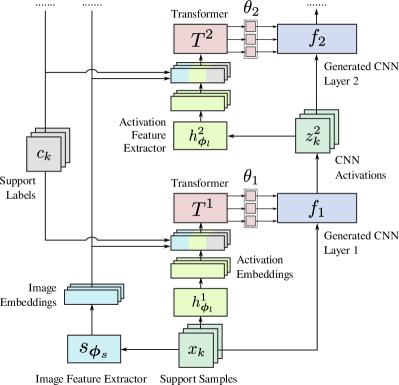
Figure 1: A diagram of our model showing the generation of two CNN layers: Transformer-based weight generators receive image embeddings $s_{\phi_{s}}(\cdot)$ and activation embeddings $h_{\phi_{l}}(\cdot)$ along with corresponding labels $c_{i}$, and produce CNN layer weights ($\theta_{1}$ and $\theta_{2}$). After being generated, the CNN model is used to compute the loss on the query set. The gradients of this loss are then used to adjust the weights of the entire weight generation model ($\phi_{s}$, $\phi_{l}$, Transformer weights).

In a special case of a one-to-one mapping from $t$ to $\tau(t)$, it is generally possible to find $\theta(\tau)$ minimizing $\mathcal{L}(\theta(\tau(t)),t)$ numerically or analytically by solving an ordinary differential equation that effectively “tracks” the local minimum of $\mathcal{L}$ along an arbitrary curve $\hat{t}:[0,1]\to\mathcal{T}$ in the task space (see Appendix B):

$$\frac{d\theta}{d\gamma}=-\left(\frac{\partial^{2}\mathcal{L}}{\partial\theta^{2}}\right)^{-1}\frac{\partial^{2}\mathcal{L}}{\partial\theta\,\partial t}\frac{d\hat{t}}{d\gamma},$$

where $\gamma\in[0,1]$ is a coordinate along the curve, $\theta(\gamma):=\theta(\tau(\hat{t}(\gamma))$, and all derivatives are computed at $\hat{t}(\gamma)$, $\theta(\gamma)$.

Empirical solution of equation 1 for $a_{\bm{\phi}}(\tau)$ represented by a deep neural network can be obtained by solving this optimization problem directly. In this section, we describe the design of the model $a_{\bm{\phi}}(\tau)$ that we call a HyperTransformer (HT). Choosing Transformer as the core component of HT, we make it possible for $a_{\bm{\phi}}$ to process any complex multi-modal task description $\tau(t)$ assuming that it can be encoded as an unordered set of Transformer tokens.

4.1 Few-Shot Learning Model

A solver $a_{\bm{\phi}}$ is the core of a few-shot learning algorithm since it encodes the knowledge of the training task distribution within its weights ${\bm{\phi}}$. We choose $a_{\bm{\phi}}$ to be a Transformer-based model (see Fig. 1) that takes a task description $\tau$ containing the information about labeled and unlabeled support-set samples as input and produces weights for some or all layers $\{\theta_{\ell}|\ell\in[1,L]\}$ of the generated CNN model. Layer weights that are not generated are instead learned end-to-end together with HT weights as ordinary task-agnostic variables. In other words, these learned layers are modified during the training phase and remain static during the evaluation phase (i.e. not dependent of the support set). In our experiments generated CNN models contain a set of convolutional layers and a final fully-connected logits layer. Here $\theta_{\ell}$ are the parameters of the $\ell$-th layer and $L$ is the total number of layers including the final logits layer (with index $L$). The weights are generated layer-by-layer starting from the first layer: $\theta_{1}(\tau)\to\theta_{2}(\theta_{1};\tau)\to\dots\to\theta_{L}(\theta_{1,\dots,L-1};\tau)$. Here we use $\theta_{a,\dots,b}$ as a short notation for $(\theta_{a},\theta_{a+1},\dots,\theta_{b})$.

Image and activation embeddings.

The weights for the layer $\ell$ are either: (a) simply learned as a task-agnostic trainable variable, or (b) generated by the Transformer that receives a concatenation of image embeddings, activation embeddings and support sample labels $c_{i}$:

$$\mathcal{I}^{\ell}:=\left\{\Big{(}\,\,s_{{\bm{\phi}}_{s}}(x_{i}),\,\,h_{{\bm{\phi}}_{l}}^{\ell}\big{(}z_{i}^{\ell}\big{)},\,\,c_{i}\,\,\Big{)}\right\}_{i=1,\dots,kn}.$$

The activation embeddings at layer $\ell$ are produced by a convolutional feature extractor $h_{{\bm{\phi}}_{l}}^{\ell}(z^{\ell}_{i})$ applied to the activations of the previous layer $z_{i}^{\ell}:=f_{\ell-1}(x_{i};\theta_{1,\dots,\ell-1})$ for $\ell>1$ and $z_{i}^{1}:=x_{i}$. The intuition behind using the activation embeddings is that the choice of the layer weights should primarily depend on the inputs received by this layer.

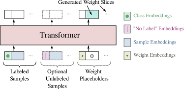
Figure 2: Structure of the tokens passed to and received from a Transformer model. Both labeled and unlabeled (optional) samples can be passed to the Transformer as inputs. Empty output tokens indicate ignored outputs.

The image embeddings are produced by a separate trainable convolutional neural network $s_{{\bm{\phi}}_{s}}(x_{i})$ that is shared by all the layers. Their purpose are to modulate each layer’s weight generator with a global high-level view of the sample that, unlike the activation embedding, is independent of the generated weights and is shared between generators.

Encoding and decoding Transformer inputs and outputs.

In the majority of our experiments, the input samples were encoded by concatenating image and activation embeddings from $\mathcal{I}^{\ell}$ to trainable label embeddings $\xi(c)$ with $\xi:[1,n]\to\mathbb{R}^{d}$. Here $n$ is the number of classes per episode and $d$ is a chosen size of the label encoding. Note that the class embeddings do not contain semantic information, but rather act as placeholders to differentiate between distinct classes. In addition to supervised few-shot learning, we also considered a semi-supervised scenario when some of the support samples are provided without the associated class information. Such unlabeled samples were fed into the Transformer using the same general encoding approach, but we used an auxiliary learned “unlabeled” token $\hat{\xi}$ in place of the label encoding $\xi(c)$ to indicate the fact that the class of the sample is unknown.

Along with the input samples, the sequence passed to the Transformer was also populated with special learnable placeholder tokens, each associated with a particular slice of the to-be-generated weight tensor. Each such token was a learnable $d$-dimensional vector padded with zeros to the size of the input sample token. After the entire input sequence was processed by the Transformer, we read out model outputs associated with the weight slice placeholder tokens and assembled output weight slices into the final weight tensors (see Fig. 2).

In our experiments we considered two different ways of encoding $k\times k\times n_{\rm input}\times n_{\rm output}$ convolutional kernels: (a) “output allocation” generates $n_{\rm output}$ tokens with weight slices of size $k^{2}\times n_{\rm input}$ and (b) “spatial allocation” generates $k^{2}$ weight slices of size $n_{\rm input}\times n_{\rm output}$. We show comparison results in Supplementary Materials.

Training the model.

The weight generation model uses the support set to produce the weights of some or all CNN model layers. Then, the cross-entropy loss is computed for the query set samples that are passed through the generated CNN model. The weight generation parameters ${\bm{\phi}}$ (including the Transformer model and image/activation feature extractor weights) are learned by optimizing this loss functwion using stochastic gradient descent.

Dataset	Approach	1-shot (channels)					5-shot (channels)
		$8$	$16$	$32$	$48$	$64$	$8$	$16$	$32$	$48$	$64$
Omniglot	MAML++	$81.4$	$88.6$	$\mathbf{95.6}$	$\mathbf{95.8}$	$\mathbf{97.7}^{\dagger}$	$83.2$	$94.9$	$\mathbf{98.6}$	$\mathbf{98.8}$	$\mathbf{99.3}^{\dagger}$
	HT	$\mathbf{87.2}$	$\mathbf{93.7}$	$\mathbf{95.5}$	$\mathbf{95.7}$	$96.2$	$\mathbf{94.7}$	$\mathbf{98.0}$	$\mathbf{98.6}$	$\mathbf{98.8}$	$98.8$
miniImageNet	MAML++	$43.9$	$46.6$	$49.4$	$52.2^{\dagger}$	–	$\mathbf{59.0}$	$\mathbf{64.6}$	$\mathbf{66.8}$	$68.3^{\dagger}$	–
	RFS	$44.0$	$49.4$	$51.5$	$54.2$	–	$56.1$	$63.5$	$\mathbf{67.1}$	$\mathbf{69.1}$	–
	HT	$\mathbf{45.5}$	$\mathbf{50.2}$	$\mathbf{53.8}$	$\mathbf{55.1}$	–	$\mathbf{59.3}$	$64.2$	$\mathbf{67.1}$	$68.1$	–
tieredImageNet	RFS	$44.1$	$47.7$	$51.5$	$54.6$	$\mathbf{56.8}^{\star}$	$55.5$	$62.0$	$66.3$	$69.3$	$73.2^{\star}$
	HT	$\mathbf{49.1}$	$\mathbf{51.9}$	$\mathbf{54.0}$	$\mathbf{55.0}$	$56.3$	$\mathbf{61.9}$	$\mathbf{65.8}$	$\mathbf{70.2}$	$\mathbf{71.1}$	$\mathbf{73.9}$

Table 1: Comparison of HT with MAML++ and RFS on models of different sizes and different datasets: (a) 20-way Omniglot, (b) 5-way miniImageNet and (c) 5-way tieredImageNet. Results for MAML++ and RFS were obtained using GitHub codes accompanying Antoniou et al. (2019) and Tian et al. (2020) correspondingly (results marked with $\dagger$ and $\star$ were taken from corresponding papers). HT generally outperforms both MAML++ and RFS for smaller models. Accuracy confidence intervals: Omniglot – between $0.1\%$ and $0.3\%$, miniImageNet and tieredImageNet – between $0.2\%$ and $0.5\%$.

4.2 Reasoning Behind the Self-Attention Mechanism

The choice of self-attention mechanism for the weight generator is not random. One reason behind this choice is that the output produced by generator with the basic self-attention is by design invariant to input permutations, i.e., permutations of samples in the training dataset. This also makes it suitable for processing unbalanced batches and batches with a variable number of samples (see Sec. 5.3). Now we show that the calculation performed by a self-attention model with properly chosen parameters can mimic basic few-shot learning algorithms further motivating its utility.

Supervised learning.

Self-attention in its rudimentary form can implement a method similar to cosine-similarity-based sample weighting encoded in the logits layer with weights $W_{i,j}\sim\sum_{m=1}^{n}y_{i}^{(m)}e_{j}^{(m)}$ which can also be viewed as a result of applying a single gradient descent step on the cross-entropy loss (see Appendix A). Here $n$ is the total number of support-set samples $\{x^{(m)}|m\in[1,n]\}$ and ${\bm{e}}^{(m)}$, ${\bm{y}}^{(m)}$ are the embedding vector and the one-hot label corresponding to $x^{(m)}$.

The approach can be outlined (see more details in Appendix A) as follows. The self-attention operation receives encoded input samples $\mathcal{I}_{k}=(\xi(c_{k}),{\bm{e}}_{k})$ and weight placeholders $(\mu(i),0)$ as its input. If each weight slice $W_{i,\cdot}$ represented by a particular token $(\mu(i),0)$ produces a query $Q_{i}$ that only attends to keys $K_{k}$ corresponding to samples $\mathcal{I}_{k}$ with labels $c_{k}$ matching $i$ and the values of these samples are set to their embeddings ${\bm{e}}_{k}$, then the self-attention operation will essentially average the embeddings of all samples assigned label $i$ thus matching the first term in ${\bm{W}}$.

Semi-supervised learning.

A similar self-attention mechanism can also be designed to produce logits layer weights when the support set contains some unlabeled samples. The proposed mechanism first propagates classes of labeled samples to similar unlabeled samples. This can be achieved by a single self-attention layer choosing the queries and the keys of the samples to be proportional to their embeddings. The attention map for sample $i$ would then be defined by a softmax of ${\bm{e}}_{i}\cdot{\bm{e}}_{j}$, or in other words would be proportional to $\exp({\bm{e}}_{i}\cdot{\bm{e}}_{j})$. Choosing sample values to be proportional to the class tokens, we can then propagate a class of a labeled sample ${\bm{e}}_{j}$ to a nearby unlabeled sample with embedding ${\bm{e}}_{i}$, for which ${\bm{e}}_{i}\cdot{\bm{e}}_{j}$ is sufficiently large. If the self-attention module is “residual”, i.e., the output of the self-attention operation is added to the original input, like it is done in the Transformer model, then this additive update would essentially “mark” an unlabeled sample by the propagated class (albeit this term might have a small norm). The second self-attention layer can then be designed similarly to the supervised case. If label embeddings are orthogonal, then even a small component of a class embedding propagated to an unlabeled sample can be sufficient for a weight slice to attend to it thus adding its embedding to the final weight (resulting in the averaging of embeddings of both labeled and proper unlabeled examples).

5 Experiments

In this section, we present HyperTransformer (HT) experimental results and discuss the implications of our empirical findings.

5.1 Datasets and Setup

Datasets.

For our experiments, we chose several most widely used few-shot datasets including Omniglot, miniImageNet and tieredImageNet. miniImageNet contains a relatively small set of labels and is arguably the simplest to overfit to. Because of this and since in many recent publications miniImageNet was replaced with a larger tieredImageNet dataset, we conduct many of our experiments and ablation studies using Omniglot and tieredImageNet.

miniImageNet						tieredImageNet
Method	1-S	5-S	Method	1-S	5-S	Method	1-S	5-S
HT	$54.1$	$68.5$	HT-48	$\mathbf{55.1}$	$68.1$	HT-32	$\mathbf{54.0}$	$\mathbf{70.2}$
MN	$43.6$	$55.3$	SAML	$52.2$	$66.5$	MAML-32	$51.7$	$\mathbf{70.3}$
IMP	$49.2$	$64.7$	GCR	$53.2$	$\mathbf{72.3}$	HT	$\mathbf{56.3}$	$\mathbf{73.9}$
PN	$49.4$	$68.2$	KTN	$54.6$	$71.2$	PN	$53.3$	$72.7$
MELR	$\mathbf{55.4}$	$\mathbf{72.3}$	PARN	$\mathbf{55.2}$	$71.6$	MELR	$\mathbf{56.4}$	$\mathbf{73.2}$
TAML	$51.8$	$66.1$	PPA	$54.5$	$67.9$	RN	$54.5$	71.3

Table 2: Comparison of miniImageNet and tieredImageNet 1-shot (1-S) and 5-shot (5-S) 5-way results for HT (underlined) and other widely known methods with a 64-64-64-64 model including (Tian et al., 2020): Matching Networks (Vinyals et al., 2016), IMP (Allen et al., 2019), Prototypical Networks (Snell et al., 2017), TAML (Jamal & Qi, 2019), SAML (Hao et al., 2019), GCR (Li et al., 2019a), KTN (Peng et al., 2019), PARN (Wu et al., 2019), Predicting Parameters from Activations (Qiao et al., 2018), Relation Net (Sung et al., 2018), MELR (Fei et al., 2021). We also include results for CNNs with fewer channels (“-32” for 32-channel models, etc.).

Models.

HyperTransformer can in principle generate arbitrarily large weight tensors by producing low-dimensional embeddings that can then be fed into another trainable model to generate the entire weight tensors. In this work, however, we limit our experiments to HT models that generate weight tensor slices encoding individual output channels directly. For the target models we focus on 4-layer CNN architectures identical to those used in MAML++ and numerous other papers. More precisely, we used a sequence of four $3\times 3$ convolutional layers with the same number of output channels followed by batch normalization (BN) layers, nonlinearities and max-pooling stride-2 layers. All BN variables were learned and not generated. Experiments with generated BN variables did not show much difference with this simpler approach. Generating larger architectures such as ResNet and WideResNet will be the subject of our future work.

5.2 Supervised Results with Logits Layer Generation

As discussed in Section 4.2, using a simple self-attention mechanism to generate the CNN logits layer can be a basis of a simple few-shot learning algorithm. Motivated by this observation, in our first experiments, we compared the proposed HT approach with MAML++ and RFS (Tian et al., 2020) on Omniglot, miniImageNet and tieredImageNet datasets (see Table 1) with HT limited to generating only the final fully-connected logits layer.

In our experiments, the dimensionality of the activation embedding was chosen to be the same as the number of model channels and the image embedding had a dimension of $32$ regardless of the model size. The image feature extractor was a simple 4-layer convolutional model with batch normalization and stride-$2$ $3\times 3$ convolutional kernels. The activation feature extractors were two-layer convolutional models with outputs of both layers averaged over the spatial dimensions and concatenated to produce the final activation embedding. For all tasks except 5-shot miniImageNet our Transformer had $3$ layers, used a simple sequence of encoder layers (Figure 2) and used the “output allocation” of weight slices (Section 4.1). Experiments with the encoder-decoder Transformer architecture can be found in Appendix E. The 5-shot miniImageNet and tieredImageNet results presented in Table 1 were obtained with a simplified Transformer model that had 1 layer, and did not have the final fully-connected layer and nonlinearity. This proved necessary for reducing model overfitting of this smaller dataset. Other model parameters are described in detail in Appendix C.

Results obtained with our method in a few-shot setting (see Table 1) are frequently better than MAML++ and RFS results, especially on smaller models, which can be attributed to parameter disentanglement between the weight generator and the CNN model. While the improvement over MAML++ and RFS gets smaller with the growing size of the generated CNN, our results for large models appear to be comparable to those obtained with MAML++, RFS and numerous other methods (see Table 2). Discussion of additional comparisons to LGM-Net (Li et al., 2019b) and LEO (Rusu et al., 2019) using a different setup (which is why they could not be included in Table 2) and showing an almost identical performance can be found in Appendix D.

While the learned HT model could perform a relatively simple calculation on high-dimensional sample embeddings, our brief analysis of the parameters space (see Appendix E) shows that using simpler 1-layer Transformers leads to a modest decrease of the test accuracy and a greater drop in the training accuracy for smaller models. However, in our experiments with 5-shot miniImageNet dataset, which is generally more prone to overfitting, we observed that increasing the Transformer model complexity improves the model training accuracy (on episodes that only use classes seen at the training time), but the test accuracy relying on classes unseen at the training time, generally degrades. We also observed that the results in Table 1 could be improved even further by increasing the embedding sizes (see Appendix E), but we did not pursue an exhaustive optimization in the parameter space.

Note that overfitting characterized by a good performance on tasks composed of seen categories, but poor generalization to unseen categories, may still have practical applications for pesonalization. Specifically, if the actual task relies on classes seen at the training time, we can generate an accurate model customized to a particular task in a single pass without having to perform any SGD steps to fine-tune the model. This is useful if, for example, the client model needs to be adjusted to a particular set of known classes most widely used by this client. We also anticipate that with more complex data augmentations and additional synthetic tasks, more complex Transformer-based models can further improve their performance on the test set.

5.3 Semi-Supervised Results

$(u,L_{T})$	1-shot	5-shot	$(2,3)$	$(4,1)$	$(4,2)$	$(4,3)$	$(9,3)$
Accuracy	$56.0$	$69.9$	$58.3$	$56.6$	$59.9$	$59.9$	$61.5$

Table 3: Test accuracy on tieredImageNet of supervised 1-shot and 5-shot models and semi-supervised 1-shot models with $u$ additional unlabeled samples per class. The weight generation Transformer model uses $3$ encoder layer for supervised tasks and $L_{T}$ encoder layers in semi-supervised experiments. Notice a performance improvement of semi-supervised learning over the 1-shot supervised results. Accuracy is seen to grow with the number of unlabeled samples and the maximum accuracy is reached when the encoder has at least two layers.

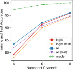
Figure 3: 5-shot-20-way Omniglot training/test accuracies as a function of the CNN model complexity: only the final logits layer being generated (logits), all layers being generated (all), training the model on all available samples for a random set of few classes (oracle). A model that generates CNN weights by memorizing all samples (being able to determine their classes) and also memorizing optimal trained weights for any selection of classes would reach the oracle accuracy, but would not generalize.

In our approach, the weight generation model is trained by optimizing the query set loss and therefore any additional information about the task, including unlabeled samples, can be provided as a part of the task description $\tau$ to the weight generator without having to alter the optimization objective. This allows us to tackle a semi-supervised few-shot learning problem without making any substantial changes to the model or the training approach. In our implementation, we simply added unlabeled samples into the support set and marked them with an auxiliary learned “unlabeled” token $\hat{\xi}$ in place of the label encoding $\xi(c)$.

Since Omniglot is typically characterized by very high accuracies in the $97\%$–$99\%$ range, we conducted all our experiments with tieredImageNet. As shown in Table 3, adding unlabeled samples results in a substantial increase of the final test accuracy. Furthermore, notice that the model achieves its best performance when the number of Transformer layers is greater than one. This is consistent with the basic mechanism discussed in Section 4.2 that required two self-attention layers to function.

It is worth noticing that adding more unlabeled samples into the support set makes our model more difficult to train and it gets stuck producing CNNs with essentially random outputs. Our solution was to introduce unlabeled samples incrementally during training. This was implemented by masking out some unlabeled samples in the beginning of the training and then gradually reducing the masking probability over time.

Layer 1                    Layer 2                    Layer 3                    Layer 4                    All layers

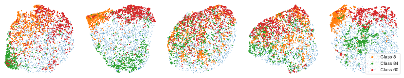
Figure 4: UMAP embedding of weights for each convolutional layer of a 6-channel CNN generated by HT for $1\,242$ different episodes from tieredImageNet. Each point corresponds to 2d embedding of the combined weights for a given layer (or concatenated for all layers) generated for a given episode. We color some of the point according to the classes contained in the episodes. For highlighted classes, the generated weights appear to be correlated between episodes where these classes are present. We selected classes specifically to demonstrate this correlation. For most of the other classes, this correlation was minor. Note that since there are 5 classes in each episode, the coloring for some of the episodes might be ambiguous. See Appendix G for more classes and samples for each class.

5.4 Generating Additional Model Layers

We demonstrated that HT model can outperform MAML++ on common few-shot learning datasets by generating just the last logits layer of the CNN model. But is it advantageous to be generating additional CNN layers (ultimately fully utilizing the capability of the HT model)?

We explored this question by comparing the performance of models, in which all, or only some of the convolutional layers were generated, while others were learned (typically all or few first convolutional layers of the CNN). We observed a significant performance improvement for models that generated all convolutional layers in addition to the CNN logits layer, but only for CNN models below a particular size. For Omniglot dataset, we saw that both training and test accuracies for a 4-channel and a 6-channel CNNs increased with the number of generated layers (see Fig. 3 and Table 4 in Appendix) and using more complex Transformer models with $2$ or more encoder layers improved both training and test accuracies of fully-generated CNN models of this size (see Appendix E). However, as the size of the model increased and reached $8$ channels, generating the last logits layer alone proved to be sufficient for getting the best results on Omniglot and tieredImageNet. By separately training an “oracle” CNN model using all available data for a random set of $n$ classes, we observed the gap between the training accuracy of the generated model and the oracle model (see Fig. 3), indicating that the Transformer does not fully capture the dependence of the optimal CNN model weights on the support set samples. A hypothetical weight generator reaching maximum training accuracy could, in principle, memorize all training images being able to associate them with corresponding classes and then generate an optimal CNN model for a particular set of classes in the episode matching “oracle” model performance.

We visualized the distribution of the weights generated by HT for different episodes by using UMAP (McInnes et al., 2018) embeddings of the generated weights for a 6-channel CNN model (see Fig. 4). We highlighted some of the classes present in the evaluation set and while the general structure may be hard to interpret, the distribution of the highlighted classes is somewhat clustered indicating the importance of semantic information for generated CNN weights. More details can be found in Appendix G.

The positive effect of generating convolutional layers can also be observed in shallow models with large convolutional kernels and large strides where the model performance can be much more sensitive to a proper choice of model weights. For example, in a 16-channel model with two convolutional kernels of size $9$ and the stride of $4$, the overall test accuracy for a model generating only the final convolutional layer was about $1\%$ lower than the accuracies of the models generating at least one additional convolutional filter. We also speculate that as the complexity of the task increases, generating some or all intermediate network layers should become more important for achieving optimal performance. Verifying this hypothesis and understanding the “boundary” in the model space between two regimes where a static backbone is sufficient or not will be the subject of our future work.

6 Conclusions

In this work, we proposed a HyperTransformer (HT), a novel Transformer-based model that generates all weights of a CNN model directly from a few-shot support set. This approach allowed us to use a high-capacity model for encoding task-dependent variations in the weights of a smaller model. We demonstrated that generating the last logits layer alone, the Transformer-based weight generator beats or matches performance of multiple traditional learning methods on several few-shot benchmarks and surpasses MAML++ and RFS performance on smaller models. More importantly, we showed that HT can be straightforwardly extended to handle more complex problems like semi-supervised tasks with unlabeled samples present in the support set. Our experiments demonstrated a considerable few-shot performance improvement in the presence of unlabeled data. Finally, we explored the impact of the Transformer-encoded model diversity in CNN models of different sizes. We used HT to generate some or all convolutional kernels and biases and showed that for sufficiently small models, adjusting all model parameters further improves their few-shot learning performance.

Appendix A Example of a Self-Attention Mechanism for Supervised Learning

Self-attention in its rudimentary form can implement a cosine-similarity-based sample weighting, which can also be viewed as a simple 1-step MAML-like learning algorithm. This can be seen by considering a simple classification model

$$f(x;\theta)=s({\bm{W}}{\bm{e}}(x;\phi)+{\bm{b}})$$

with $\theta=({\bm{W}},{\bm{b}},\phi)$, where ${\bm{e}}(x;\phi)$ is the embedding and $s(\cdot)$ is a softmax function. MAML algorithm identifies such initial weights $\theta_{0}$ that given any task $T$ just a few gradient descent steps with respect to the loss $\mathcal{L}_{T}$ starting at $\theta_{0}$ bring the model towards a task-specific local optimum of $\mathcal{L}_{T}$.

Notice that if any label assignment in the training tasks is equally likely, it is natural for $f(x;\theta_{0})$ to not prefer any particular label over the others. Guided by this, let us choose ${\bm{W}}_{0}$ and ${\bm{b}}_{0}$ that are label-independent. Substituting $\theta=\theta_{0}+\delta\theta$ into $f(x;\theta)$, we obtain

$$f_{\ell}(x;\theta)=f_{\ell}(x;\theta_{0})+s_{\ell}^{\prime}(\cdot)(\delta{\bm{W}}_{\ell}{\bm{e}}(x;\phi_{0})+\delta{\bm{b}}_{\ell}+{\bm{W}}_{0,\ell}{\bm{e}}^{\prime}(x;\phi_{0})\delta\phi)+O(\delta\theta^{2}),$$

where $\ell$ is the label index and $\delta\theta=(\delta{\bm{W}},\delta{\bm{b}},\delta\phi)$. We see that the lowest-order label-dependent correction to $f_{\ell}(x;\theta_{0})$ is given simply by $s_{\ell}^{\prime}(\cdot)(\delta{\bm{W}}_{\ell}{\bm{e}}(x;\phi_{0})+\delta{\bm{b}}_{\ell})$. In other words, in the lowest-order, the model only adjusts the final logits layer to adapt the pretrained embedding ${\bm{e}}(x;\phi_{0})$ to a new task. It is then easy to calculate that for a simple softmax cross-entropy loss, a single step of the gradient descent results in the following logits weight and bias updates:

$$\delta W_{ij}=\frac{\gamma}{n}\sum_{m=1}^{n}\left(y_{i}^{(m)}-\frac{1}{|C|}\right)e_{j}(x^{(m)};\phi_{0}),\qquad\delta b_{i}=\frac{\gamma}{n}\sum_{m=1}^{n}\left(y_{i}^{(m)}-\frac{1}{|C|}\right).$$ (2)

Here $\gamma$ is the learning rate, $n$ is the total number of support-set samples, $|C|$ is the number of classes and ${\bm{y}}^{(m)}$ is the one-hot label corresponding to $x^{(m)}$. A closely-related idea of extending the logits layer with a vector proportional to an average of the novel class sample embeddings is used in the “imprinted weights” approach (Qi et al., 2018) allowing to add novel classes into pre-trained models.

Now consider a self-attention module generating the last logits layer and acting on a sequence of processed input samples $\mathcal{I}^{L}=\{(\,\xi(c_{i})\,,\,h_{{\bm{\phi}}_{l}}(e_{i})\,)\}_{i=1,\dots,n}$ and weight placeholders $\mathcal{W}^{L}:=\{(\,\mu(k)\,,\,0\,)\}_{k=1,\dots,|C|}$, where $|C|$ is the number of classes and also the number of weight slices of ${\bm{W}}$ if each slice corresponds to an output layer channel. The output of a simple self-attention module for the weight slice with index $i$ is then given by:

$$Z^{-1}\sum_{m=1}^{n}e^{{\bm{Q}}(\mathcal{W}^{L}_{i})\cdot{\bm{K}}_{I}(\mathcal{I}^{L}_{m})}{\bm{V}}_{I}(\mathcal{I}^{L}_{m})+Z^{-1}\sum_{m=1}^{N_{w}}e^{{\bm{Q}}(\mathcal{W}^{L}_{i})\cdot{\bm{K}}_{W}(\mathcal{W}^{L}_{m})}{\bm{V}}_{W}(\mathcal{W}^{L}_{m}),$$ (3)

where $Z:=\sum_{m=1}^{n}e^{{\bm{Q}}(\mathcal{W}^{L}_{i})\cdot{\bm{K}}_{I}(\mathcal{I}^{L}_{m})}+\sum_{m=1}^{N_{w}}e^{{\bm{Q}}(\mathcal{W}^{L}_{i})\cdot{\bm{K}}_{W}(\mathcal{W}^{L}_{m})}$. It is easy to see that with a proper choice of query and key matrices attending only to prepended $\xi$ and $\mu$ tokens, the second term in equation 3 can be made negligible, while ${\bm{Q}}(\mathcal{W}^{L}_{i})\cdot{\bm{K}}_{I}(\mathcal{I}^{L}_{m})$ can make the softmax function only attend to those components of ${\bm{V}}_{I}$ that correspond to samples with label $i$. Choosing ${\bm{V}}_{I}(\mathcal{I}^{L}_{m})$ to be proportional to ${\bm{e}}_{m}$, we can then recover the first term in $\delta{\bm{W}}$ in equation 2. The second term in $\delta{\bm{W}}$ can be produced, for example, with the help of a second head that generates identical attention weights for all samples, thus summing up their embeddings.

Appendix B Analytical Expression for Generated Weights

Supplied with a distribution $p(t)$ of training tasks $t\in\mathcal{T}_{\rm{train}}$, we learn the weight generator $a_{\bm{\phi}}$ by optimizing the following objective:

$$\operatorname*{arg\,min}_{\bm{\phi}}\mathbb{E}_{t\sim p(t)}\mathcal{L}(a_{\bm{\phi}}(\tau(t)),t).$$

If the family of functions $a_{\bm{\phi}}(\tau)$ is sufficiently rich, we can instead try solving an optimization problem of the form $\theta_{*}(\tau(t)):=\operatorname*{arg\,min}_{\theta}\mathcal{L}(\theta,t)$ with $\theta_{*}\in C^{2}$.

Generally, when $t\mapsto\tau$ is not one-to-one, it is impossible to minimize $\mathcal{L}(\theta_{*}(\tau(t)),t)$ for each $t$ because $\mathcal{L}(\cdot,t_{1})$ and $\mathcal{L}(\cdot,t_{2})$ will typically differ even if $\tau(t_{1})=\tau(t_{2})$. However, if this mapping is one-to-one, and we can re-parameterize the space of tasks $\mathcal{T}$ choosing $t$ to have the same dimension as $\tau$, the condition that $\mathcal{L}(\theta_{*}(\tau(t+\delta t)),t+\delta t)$ is an extremum for any infinitesimal $\delta t$ can be rewritten as:

$$\frac{\partial\mathcal{L}}{\partial\theta}(\theta_{*}(\tau(t+\delta t)),t+\delta t)=\frac{\partial^{2}\mathcal{L}}{\partial\theta^{2}}\frac{\partial\theta_{*}}{\partial\tau}\frac{\partial\tau}{\partial t}\delta t+\frac{\partial^{2}\mathcal{L}}{\partial\theta\,\partial t}\delta t+O(\delta t^{2})=0,$$

which in turn means that:

$$\frac{\partial^{2}\mathcal{L}}{\partial\theta^{2}}\frac{\partial\theta_{*}}{\partial\tau}\frac{\partial\tau}{\partial t}=-\frac{\partial^{2}\mathcal{L}}{\partial\theta\,\partial t}.$$

If the Hessian of $\mathcal{L}$ and $\partial\tau/\partial t$ are non-singular, we can solve this equation for $\partial\theta_{*}/\partial\tau$:

$$\frac{\partial\theta_{*}}{\partial\tau}=-\left(\frac{\partial^{2}\mathcal{L}}{\partial\theta^{2}}\right)^{-1}\frac{\partial^{2}\mathcal{L}}{\partial\theta\,\partial t}\left(\frac{\partial\tau}{\partial t}\right)^{-1}.$$ (4)

Now assume that we know a solution of $\operatorname*{arg\,min}_{\theta_{*}}\mathcal{L}(\theta_{*},t)$ for some particular task $t=t_{0}$. The derivative 4 can then be used to “track” this local minimum at $t_{0}$ to any other task $t_{1}$ in a sufficiently small vicinity of $t_{0}$, where $\mathcal{L}$ remains convex and the Hessian of $\mathcal{L}$ is not singular. Choosing a path $\hat{t}:[0,1]\to\mathcal{T}$ with $\hat{t}(0)=t_{0}$ and $\hat{t}(1)=t_{1}$, we need to integrate $\partial\theta_{*}/\partial\tau$ along $\tau(\hat{t}(\gamma))$ with $\gamma$ changing from $0$ to $1$, which is equivalent to integrating the following ordinary differential equation:

$$\frac{d\theta_{*}}{d\gamma}=-\left(\frac{\partial^{2}\mathcal{L}}{\partial\theta^{2}}\right)^{-1}\frac{\partial^{2}\mathcal{L}}{\partial\theta\,\partial t}\frac{d\hat{t}}{d\gamma},$$

where $\theta_{*}(\gamma)=\theta_{*}(\tau(\hat{t}(\gamma))$ and all derivatives are computed at $\hat{t}(\gamma)$ and $\theta_{*}(\gamma)$.

Appendix C Model Parameters

Here we provide additional information about the model parameters used in our experiments.

Image augmentations and feature extractor parameters.

For Omniglot dataset, we used the same image augmentations that were originally proposed in MAML. For miniImageNet and tieredImageNet datasets, however, we used ImageNet-style image augmentations including horizontal image flipping, random color augmentations and random image cropping. This helped us to avoid model overfitting on the miniImageNet dataset and possibly on tieredImageNet.

The dimensionality $d$ of the label encoding $\xi$ and weight slice encoding $\mu$ was typically set to $32$. Increasing $d$ up to the maximum number of weight slices plus the number of per-episode labels, would allow the model to fully disentangle examples for different labels and different weight slices, but can also make the model train slower.

Transformer parameters.

Since the weight tensors of each layer are generally different, our per-layer transformers were also different. The key, query and value dimensions of the transformer were chosen to be equal to a pre-defined fraction $\nu$ of the input embedding size, which in turn was a function of the label, image and activation embedding sizes and the sizes of the weight slices. The inner dimension of the final fully-connected layer in the transformer was also chosen using the same approach. In our miniImageNet and tieredImageNet experiments, $\nu$ was chosen to be $0.5$ and in Omniglot experiments, we used $\nu=1$. Each transformer typically contained $2$ or $3$ encoder layers and used $2$ or $8$ heads for Omniglot and miniImageNet, tieredImageNet, correspondingly.

Learning schedule.

In all our experiments, we used gradient descent optimizer with a learning rate in the $0.01$ to $0.02$ range. Our early experiments with more advanced optimizers were unstable. We used a learning rate decay schedule, in which we reduced the learning rate by a factor of $0.95$ every $10^{5}$ learning steps.

Appendix D Additional Supervised Experiments

While the advantage of decoupling parameters of the weight generator and the generated CNN model is expected to vanish with the growing CNN model size, we compared our approach to two other methods, LGM-Net (Li et al., 2019b) and LEO (Rusu et al., 2019), to verify that our approach can match their performance on sufficiently large models.

For our comparison with the LGM-Net method, we used the same image augmentation technique that was used in (Li et al., 2019b) where it was applied both at the training and the evaluation stages (Ma, 2019). We also used the same CNN architecture with 4 learned 64-channel convolutional layers followed by two generated convolutional layers and the final logits layer. In our weight generator, we used 2-layer transformers with activation feature extractors that relied on 48-channel convolutional layers and did not use any image embeddings. We trained our model in the end-to-end fashion on the miniImageNet 1-shot-5-way task and obtained a test accuracy of $69.3\%\pm 0.3\%$ almost identical to the $69.1\%$ accuracy reported in (Li et al., 2019b).

We also carried out a comparison with LEO by using our method to generate a fully-connected layer on top of the tieredImageNet embeddings pre-computed with a WideResNet-28 model employed by (Rusu et al., 2019). For our experiments, we used a simpler 1-layer transformer model with 2 heads that did not have the final fully-connected layer and nonlinearity. We also used $L_{2}$ regularization of the generated fully-connected weights setting the regularization weight to $10^{-3}$. As a result of training this model, we obtained $66.2\%\pm 0.2\%$ and $81.6\%\pm 0.2\%$ test accuracies on the 1-shot-5-way and 5-shot-5-way tieredImageNet tasks correspondingly. These results are almost identical to $66.3\%$ and $81.4\%$ accuracies reported in (Rusu et al., 2019).

Appendix E Dependence on Parameters and Ablation Studies

Most of our parameter explorations were conducted for Omniglot dataset. We chose a 16-channel model trained on a 1-shot-20-way Omniglot task as an example of a model, for which just the logits layer generation was sufficient. We also chose a 4-channel model trained on a 5-shot-20-way Omniglot task for the role of a model, for which generation of all convolutional layers proved to be beneficial. Figures 6 and 7 show comparison of training and test accuracies on Omniglot for different parameter values for these two models. Here we only used two independent runs for each parameter value, which did not allow us to sufficiently reduce the statistical error. Despite of this, in the following, we try to highlight a few notable parameter dependencies. Note here that in some experiments with particularly large embedding or model sizes, training progressed beyond the target number of steps and there could also be overfitting for very large models.

Number of transformer layers.

Increasing the number of transformer layers is seen to be particularly important in the 4-channel model. The 16-channel model also demonstrates the benefit of using $1$ vs $2$ transformer layers, but the performance appears to degrade when we use $3$ transformer layers.

Activation embedding dimension.

Particularly, small activation embeddings can be seen to hurt the performance in both models, while using larger activation embeddings appears to be advantageous in most cases except for the 32-dimensional activation embeddings in the 4-channel model.

Class embedding dimension.

Particularly low embedding dimension of 16 can be seen to hurt the performance of both models.

Number of transformer heads.

Increasing the number of transformer heads leads to performance degradation in the 16-channel model, but does not have a pronounced effect in the 4-channel model.

Image embedding dimensions.

Removing the image embedding, or using an 8-dimensional embedding can be seen to hurt the performance in both cases of the 4- and 16-channel models.

Transformer architecture.

While the majority of our experiments were conducted with a sequence of transformer encoder layers, we also experimented with an alternative weight generation approach, where both encoder and decoder transformer layers were employed (see Fig. 5). Our experiments with both architectures suggest that the role of the decoder is pronounced, but very different in two models: in the 16-channel model, the presence of the decoder increases the model performance, while in the 4-channel model, it leads to accuracy degradation.

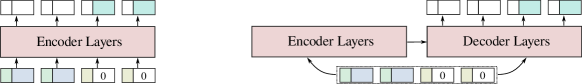
Figure 5: Two transformer-based approaches to weight generation studied in our experiments: only encoder layers (left), encoder and decoder layers on the same input sequence (right).

Inner transformer embedding sizes.

Varying the $\nu$ parameter for different components of the transformer model (key/query pair, value and inner fully-connect layer size), we quantify their importance on the model performance. Using very low $\nu$ for the value dimension hurts performance of both models. The effect of key/query and inner dimensions can be distinctly seen only in the 4-channel model, where using $\nu=1$ or $\nu=1.5$ appears to produce the best results.

Weight allocation approach.

Our experiments with the “spatial” weight allocation in 4- and 16-channel models showed slightly inferior performance (both accuracies dropping by about $0.2\%$ to $0.4\%$ in both experiments) compared to that obtained with the “output” weight allocation method.

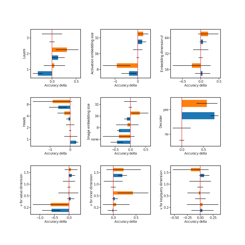
Figure 6: Change of the training (blue) and test (orange) accuracies on 1-shot-20-way Omniglot task for a 16-channel model relative to the base configuration with 3-layer transformer, 16-dimensional activation embedding, $\nu=1.0$, $d=32$, $2$ heads and 32-dimensional image embedding. Approximate confidence intervals are shown.

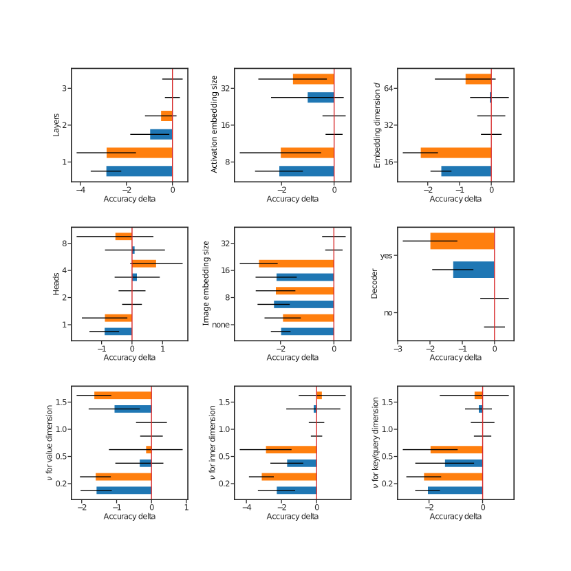
Figure 7: Change of the training (blue) and test (orange) accuracies on 5-shot-20-way Omniglot task for a 4-channel model relative to the base configuration with 3-layer transformer, 16-dimensional activation embedding, $\nu=1.0$, $d=32$, $2$ heads and 32-dimensional image embedding. Approximate confidence intervals are shown.

Appendix F Attention maps of learned transformer models

We visualized the attention maps of several transformer-based models that we used for CNN layer generation. Figure 8 shows attention maps for a 2-layer 4-channel CNN network generated using a 1-head 1-layer transformer on miniImageNet(labeled samples are sorted in the order of their episode labels). Attention map for the final logits layer (“CNN Layer 3”) is seen to exhibit a “stairways” pattern indicating that a weight slice $W_{c,\cdot}$ for episode label $c$ is generated by attending to all samples except for those with label $c$. This is reminiscent of the supervised learning mechanism outlined in Sec. 4.2. While the proposed mechanism would attend to all samples with label $c$ and average their embeddings, another alternative is to average embeddings of samples with other labels and then invert the result. We hypothesize that the trained transformer performs a similar calculation with additional learned transformer parameters, which may be seen to result in mild fluctuations of the attention to different input samples.

The attention maps for a semi-supervised learning problem with a 2-layer transformer is shown in Figure 9. One thing to notice is that a mechanism similar to the one described above appears to be used in the first transformer layer, where weight slices $W_{c,\cdot}$ attend to all labeled samples with labels $c_{i}\neq c$. At the same time, unlabeled samples can be seen to attend to labeled samples in layer 1 (see “Unlabeled” rows and “Label …” columns) and the weight slices in layer 2 then attend to the updated unlabeled sample tokens (see “Weights” rows and “Unlabeled” columns in the second layer). This additional pathway connecting labeled samples to unlabeled samples and finally to the logits layer weights is again reminiscent of the simplistic semi-supervised learning mechanism outlined in Sec. 4.2.

The exact details of these calculations and the generation of intermediate convolutional layers is generally much more difficult to interpret just from the attention maps and a more careful analysis of the trained model is necessary to draw the final conclusions.

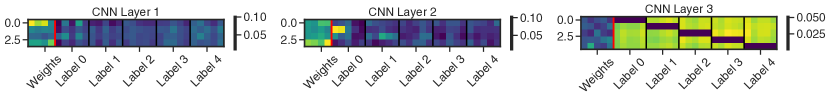
Figure 8: Learned attention maps for 2-layer 4-channel CNN network generated with 1 head, 1 layer transformer for 5-shot miniImageNet.

Transformer Layer 1	Transformer Layer 2

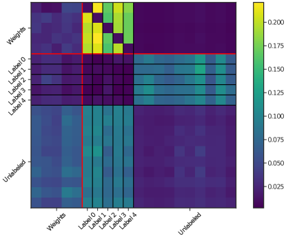
Figure 9: Learned attention maps for 4-layer 8-channel CNN network generated with 1-head, 2-layer transformer for 5-shot tieredImageNet with additional unsupervised samples (2 per class). Only the last layer of CNN is generated.

Appendix G UMAP embedding of the generated weights.

	Layer 1              Layer 2              Layer 3              Layer 4              All layers
Class 10               Class 85            Class 39               Class 60             Class 84                Class 8

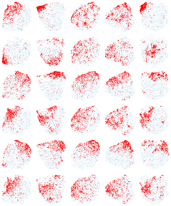
Figure 10: UMAP embedding of weights generated by the HyperTransformer. Each point corresponds to the embedding of the weights of a given layer for a given episode. The original dimensionality for the first layer weights is $162=3\times 3\times 3\times 6$, for each subsequent weights is $324=3\times 3\times 6\times 6$ and for all layers combined is 1 134. We further selected 6 different classes with the smallest standard deviation in the embeddings and highlighted the episodes that contain these classes.

Class 8
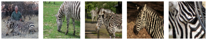
Class 84
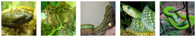
Class 60
Class 39
Class 85
Class 10

Figure 11: Examples of classes from tieredImageNet that we used to highlight in UMAP embedding.

Figure 10 shows additional plots of the UMAP embedding with some of the classes highlighted. Here, we can more clearly see that, at least for those classes, the embedding is quite correlated with the episodes where these classes are included. This suggests that the HyperTransformer does generate meaningful individualized weights for each of the episode. Figure 11 shows some samples of the highlighted classes. Notice that Class 8 is clustered more tightly for the second layer, which means that the weights for the episodes containing this class are much more similar specifically for that layer. Indeed, Class 8 corresponds to zebras, with their stripes pattern being a distinct feature. In order to be able to distinguish this feature, CNN would need to aggregate information from a wide field of view. This would probably not happen in the first layer, thus we see almost no correlation for the first one, but very tight cluster for the second.

Appendix H Visualization of the Generated CNN Weights.

Figures 12 and 13 show the examples of the CNN kernels that are generated by a single-head, 1-layer transformer for a simple 2-layer CNN model with $9\times 9$ stride-4 kernels. Different figures correspond to different approaches to re-assembling the weights from the generated slices: using “output” allocation or “spatial” allocation (see Section 4.1 in the main text for more information). Notice that “spatial” weight allocation produces more homogeneous kernels for the first layer when compared to the “output” allocation. In both figures we show the difference of the final generated kernels for 3 variants: model with both layers generated, one generated and one trained and both trained.

Trained layers are always fixed for the inference for all the episodes, but the generated layers vary, albeit not significantly. In Figures 14 and 15 we show the generated kernels for two different episodes and, on the right, the difference between them. It appears that the generated convolutional kernel change withing $10-15\%$ form episode to episode.

	Generated/Generated	Trained/Generated	Trained/Trained
CNN Layer 1
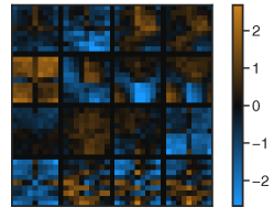
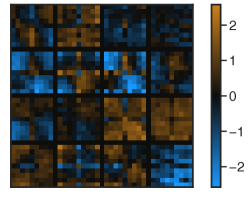
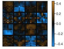
CNN Layer 0

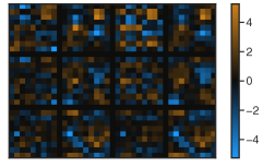
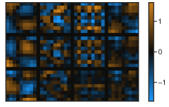
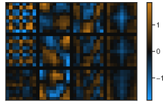
Figure 12: Visualizing convolutional kernels for a 2-layer network with a $9\times 9$ CNN kernel size and stride of 4 trained on miniImageNet. Each column shows 1 model with two layers and fully-connected head that is always generated by the transformer. Left: both CNN layers are generated, center: first CNN layer is trained, second is generated, right: both CNN layers are trained. Layer weight allocation: “output”.

	Generated/Generated	Trained/Generated	Trained/Trained
CNN Layer 1
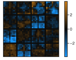
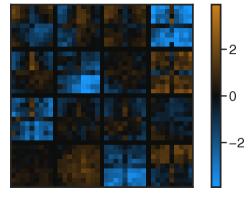
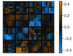
CNN Layer 0

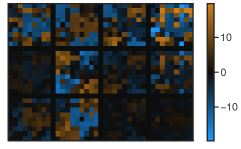
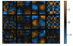
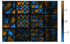
Figure 13: Visualizing convolutional kernels for a 2-layer network with a $9\times 9$ CNN kernel size and stride of 4 trained on miniImageNet. Each column shows 1 model with two layers and fully-connected head that is always generated by the transformer. Left: both CNN layers are generated, center: first CNN layer is trained, second is generated, right: both CNN layers are trained. Layer weight allocation: “spatial”.

	Episode 0	Episode 1	Difference
Layer 1
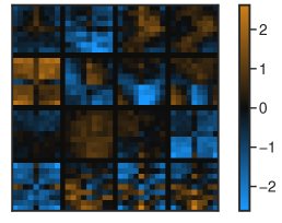
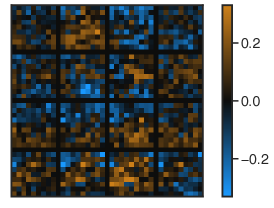
Layer 0

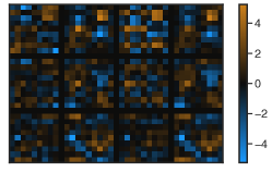
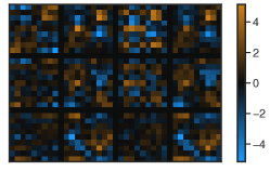
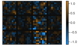
Figure 14: Visualizing generated convolutional kernels in a 2-layer model for two different episodes. Left two plots: kernels for two random episodes of 5 classes, right: the difference in generated kernels for two episodes. Layer weight allocation: “output”.

	Episode 0	Episode 1	Difference
Layer 1
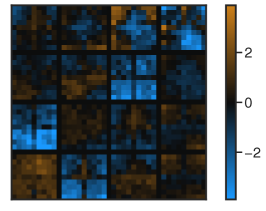
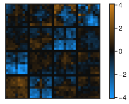
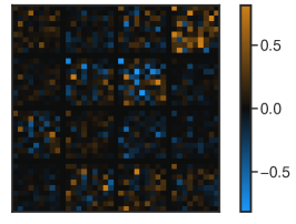
Layer 0

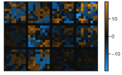
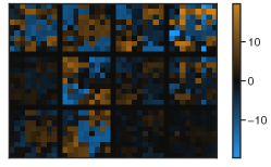
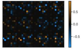
Figure 15: Visualizing generated convolutional kernels in a 2-layer model for two different episodes. Left two plots: kernels for two random episodes of 5 classes, right: the difference in generated kernels for two episodes. Layer weight allocation: “spatial”.

Appendix I Additional Tables and Figures

Table 4: Average model test and training accuracies on Omniglot (separated by a slash) for the models of different sizes. “Logits” row shows accuracies for the model with only the fully-connected logits layer generated from the support set. It can be interpreted as a method based on a learned embedding. “All” row reports accuracies of the models with some or all convolutional layers being generated. We were not able to see a statistically significant evidence of an advantage of generating more than one convolutional layers.

	4-channel	6-channel	8-channel
Logits	$77.9$ / $79.2$	$90.0$ / $91.4$	$94.4$ / $95.8$
All	$82.0$ / $83.4$	$90.7$ / $92.0$	$94.6$ / $96.0$

References

- Allen et al. (2019) Allen, K. R., Shelhamer, E., Shin, H., and Tenenbaum, J. B. Infinite mixture prototypes for few-shot learning. In Chaudhuri, K. and Salakhutdinov, R. (eds.), Proceedings of the 36th International Conference on Machine Learning, ICML 2019, 9-15 June 2019, Long Beach, California, USA, volume 97 of Proceedings of Machine Learning Research, pp. 232–241. PMLR, 2019.
- Antoniou et al. (2019) Antoniou, A., Edwards, H., and Storkey, A. J. How to train your MAML. In 7th International Conference on Learning Representations, ICLR 2019, New Orleans, LA, USA, May 6-9, 2019. OpenReview.net, 2019.
- Carion et al. (2020) Carion, N., Massa, F., Synnaeve, G., Usunier, N., Kirillov, A., and Zagoruyko, S. End-to-end object detection with transformers. In Vedaldi, A., Bischof, H., Brox, T., and Frahm, J. (eds.), Computer Vision - ECCV 2020 - 16th European Conference, Glasgow, UK, August 23-28, 2020, Proceedings, Part I, volume 12346 of Lecture Notes in Computer Science, pp. 213–229. Springer, 2020.
- Chen et al. (2021) Chen, H., Wang, Y., Guo, T., Xu, C., Deng, Y., Liu, Z., Ma, S., Xu, C., Xu, C., and Gao, W. Pre-trained image processing transformer. In IEEE Conference on Computer Vision and Pattern Recognition, CVPR 2021, virtual, June 19-25, 2021, pp. 12299–12310. Computer Vision Foundation / IEEE, 2021.
- Dosovitskiy et al. (2021) Dosovitskiy, A., Beyer, L., Kolesnikov, A., Weissenborn, D., Zhai, X., Unterthiner, T., Dehghani, M., Minderer, M., Heigold, G., Gelly, S., Uszkoreit, J., and Houlsby, N. An image is worth 16x16 words: Transformers for image recognition at scale. In 9th International Conference on Learning Representations, ICLR 2021, Virtual Event, Austria, May 3-7, 2021, 2021.
- Fei et al. (2021) Fei, N., Lu, Z., Xiang, T., and Huang, S. MELR: meta-learning via modeling episode-level relationships for few-shot learning. In 9th International Conference on Learning Representations, ICLR 2021, Virtual Event, Austria, May 3-7, 2021. OpenReview.net, 2021.
- Finn et al. (2017) Finn, C., Abbeel, P., and Levine, S. Model-agnostic meta-learning for fast adaptation of deep networks. In Precup, D. and Teh, Y. W. (eds.), Proceedings of the 34th International Conference on Machine Learning, volume 70 of Proceedings of Machine Learning Research, pp. 1126–1135. PMLR, 06–11 Aug 2017.
- Gidaris & Komodakis (2018) Gidaris, S. and Komodakis, N. Dynamic few-shot visual learning without forgetting. In 2018 IEEE Conference on Computer Vision and Pattern Recognition, CVPR 2018, Salt Lake City, UT, USA, June 18-22, 2018, pp. 4367–4375. IEEE Computer Society, 2018. doi: 10.1109/CVPR.2018.00459.
- Guo & Cheung (2020) Guo, Y. and Cheung, N. Attentive weights generation for few shot learning via information maximization. In 2020 IEEE/CVF Conference on Computer Vision and Pattern Recognition, CVPR 2020, Seattle, WA, USA, June 13-19, 2020, pp. 13496–13505. Computer Vision Foundation / IEEE, 2020.
- Ha et al. (2017) Ha, D., Dai, A. M., and Le, Q. V. HyperNetworks. In 5th International Conference on Learning Representations, ICLR 2017, Toulon, France, April 24-26, 2017, Conference Track Proceedings, 2017.
- Hao et al. (2019) Hao, F., He, F., Cheng, J., Wang, L., Cao, J., and Tao, D. Collect and select: Semantic alignment metric learning for few-shot learning. In 2019 IEEE/CVF International Conference on Computer Vision, ICCV 2019, Seoul, Korea (South), October 27 - November 2, 2019, pp. 8459–8468. IEEE, 2019. doi: 10.1109/ICCV.2019.00855.
- Jamal & Qi (2019) Jamal, M. A. and Qi, G. Task agnostic meta-learning for few-shot learning. In IEEE Conference on Computer Vision and Pattern Recognition, CVPR 2019, Long Beach, CA, USA, June 16-20, 2019, pp. 11719–11727. Computer Vision Foundation / IEEE, 2019. doi: 10.1109/CVPR.2019.01199.
- Koch et al. (2015) Koch, G., Zemel, R., Salakhutdinov, R., et al. Siamese neural networks for one-shot image recognition. In ICML deep learning workshop, volume 2. Lille, 2015.
- Li et al. (2019a) Li, A., Luo, T., Xiang, T., Huang, W., and Wang, L. Few-shot learning with global class representations. In 2019 IEEE/CVF International Conference on Computer Vision, ICCV 2019, Seoul, Korea (South), October 27 - November 2, 2019, pp. 9714–9723. IEEE, 2019a. doi: 10.1109/ICCV.2019.00981.
- Li et al. (2019b) Li, H., Dong, W., Mei, X., Ma, C., Huang, F., and Hu, B. Lgm-net: Learning to generate matching networks for few-shot learning. In Chaudhuri, K. and Salakhutdinov, R. (eds.), Proceedings of the 36th International Conference on Machine Learning, ICML 2019, 9-15 June 2019, Long Beach, California, USA, volume 97 of Proceedings of Machine Learning Research, pp. 3825–3834. PMLR, 2019b.
- Liu et al. (2021) Liu, L., Hamilton, W. L., Long, G., Jiang, J., and Larochelle, H. A universal representation transformer layer for few-shot image classification. In 9th International Conference on Learning Representations, ICLR 2021, Virtual Event, Austria, May 3-7, 2021. OpenReview.net, 2021.
- Liu et al. (2019) Liu, Y., Lee, J., Park, M., Kim, S., Yang, E., Hwang, S. J., and Yang, Y. Learning to propagate labels: Transductive propagation network for few-shot learning. In 7th International Conference on Learning Representations, ICLR 2019, New Orleans, LA, USA, May 6-9, 2019, 2019.
- Ma (2019) Ma, C. LGM-Net. https://github.com/likesiwell/LGM-Net, 2019.
- Mahabadi et al. (2021) Mahabadi, R. K., Ruder, S., Dehghani, M., and Henderson, J. Parameter-efficient multi-task fine-tuning for transformers via shared hypernetworks. In Zong, C., Xia, F., Li, W., and Navigli, R. (eds.), Proceedings of the 59th Annual Meeting of the Association for Computational Linguistics and the 11th International Joint Conference on Natural Language Processing, ACL/IJCNLP 2021, (Volume 1: Long Papers), Virtual Event, August 1-6, 2021, pp. 565–576. Association for Computational Linguistics, 2021. doi: 10.18653/v1/2021.acl-long.47.
- McInnes et al. (2018) McInnes, L., Healy, J., and Melville, J. Umap: Uniform manifold approximation and projection for dimension reduction. arXiv preprint arXiv:1802.03426, 2018.
- Nichol et al. (2018) Nichol, A., Achiam, J., and Schulman, J. On first-order meta-learning algorithms. CoRR, abs/1803.02999, 2018.
- Oreshkin et al. (2018) Oreshkin, B. N., López, P. R., and Lacoste, A. TADAM: task dependent adaptive metric for improved few-shot learning. In Bengio, S., Wallach, H. M., Larochelle, H., Grauman, K., Cesa-Bianchi, N., and Garnett, R. (eds.), Advances in Neural Information Processing Systems 31: Annual Conference on Neural Information Processing Systems 2018, NeurIPS 2018, December 3-8, 2018, Montréal, Canada, pp. 719–729, 2018.
- Peng et al. (2019) Peng, Z., Li, Z., Zhang, J., Li, Y., Qi, G., and Tang, J. Few-shot image recognition with knowledge transfer. In 2019 IEEE/CVF International Conference on Computer Vision, ICCV 2019, Seoul, Korea (South), October 27 - November 2, 2019, pp. 441–449. IEEE, 2019. doi: 10.1109/ICCV.2019.00053.
- Pilault et al. (2021) Pilault, J., Elhattami, A., and Pal, C. J. Conditionally adaptive multi-task learning: Improving transfer learning in NLP using fewer parameters & less data. In 9th International Conference on Learning Representations, ICLR 2021, Virtual Event, Austria, May 3-7, 2021. OpenReview.net, 2021.
- Qi et al. (2018) Qi, H., Brown, M., and Lowe, D. G. Low-shot learning with imprinted weights. In 2018 IEEE Conference on Computer Vision and Pattern Recognition, CVPR 2018, Salt Lake City, UT, USA, June 18-22, 2018, pp. 5822–5830. Computer Vision Foundation / IEEE Computer Society, 2018. doi: 10.1109/CVPR.2018.00610.
- Qiao et al. (2018) Qiao, S., Liu, C., Shen, W., and Yuille, A. L. Few-shot image recognition by predicting parameters from activations. In 2018 IEEE Conference on Computer Vision and Pattern Recognition, CVPR 2018, Salt Lake City, UT, USA, June 18-22, 2018, pp. 7229–7238. Computer Vision Foundation / IEEE Computer Society, 2018. doi: 10.1109/CVPR.2018.00755.
- Ratzlaff & Li (2019) Ratzlaff, N. and Li, F. Hypergan: A generative model for diverse, performant neural networks. In Chaudhuri, K. and Salakhutdinov, R. (eds.), Proceedings of the 36th International Conference on Machine Learning, ICML 2019, 9-15 June 2019, Long Beach, California, USA, volume 97 of Proceedings of Machine Learning Research, pp. 5361–5369. PMLR, 2019.
- Ravi & Larochelle (2017) Ravi, S. and Larochelle, H. Optimization as a model for few-shot learning. In 5th International Conference on Learning Representations, ICLR 2017, Toulon, France, April 24-26, 2017, Conference Track Proceedings. OpenReview.net, 2017.
- Ren et al. (2018) Ren, M., Triantafillou, E., Ravi, S., Snell, J., Swersky, K., Tenenbaum, J. B., Larochelle, H., and Zemel, R. S. Meta-learning for semi-supervised few-shot classification. In 6th International Conference on Learning Representations, ICLR 2018, Vancouver, BC, Canada, April 30 - May 3, 2018, Conference Track Proceedings, 2018.
- Requeima et al. (2019) Requeima, J., Gordon, J., Bronskill, J., Nowozin, S., and Turner, R. E. Fast and flexible multi-task classification using conditional neural adaptive processes. In Wallach, H. M., Larochelle, H., Beygelzimer, A., d’Alché-Buc, F., Fox, E. B., and Garnett, R. (eds.), Advances in Neural Information Processing Systems 32: Annual Conference on Neural Information Processing Systems 2019, NeurIPS 2019, December 8-14, 2019, Vancouver, BC, Canada, pp. 7957–7968, 2019.
- Rusu et al. (2019) Rusu, A. A., Rao, D., Sygnowski, J., Vinyals, O., Pascanu, R., Osindero, S., and Hadsell, R. Meta-learning with latent embedding optimization. In 7th International Conference on Learning Representations, ICLR 2019, New Orleans, LA, USA, May 6-9, 2019, 2019.
- Snell et al. (2017) Snell, J., Swersky, K., and Zemel, R. S. Prototypical networks for few-shot learning. In Guyon, I., von Luxburg, U., Bengio, S., Wallach, H. M., Fergus, R., Vishwanathan, S. V. N., and Garnett, R. (eds.), Advances in Neural Information Processing Systems 30: Annual Conference on Neural Information Processing Systems 2017, December 4-9, 2017, Long Beach, CA, USA, pp. 4077–4087, 2017.
- Sung et al. (2018) Sung, F., Yang, Y., Zhang, L., Xiang, T., Torr, P. H. S., and Hospedales, T. M. Learning to compare: Relation network for few-shot learning. In 2018 IEEE Conference on Computer Vision and Pattern Recognition, CVPR 2018, Salt Lake City, UT, USA, June 18-22, 2018, pp. 1199–1208. IEEE Computer Society, 2018. doi: 10.1109/CVPR.2018.00131.
- Tay et al. (2021) Tay, Y., Zhao, Z., Bahri, D., Metzler, D., and Juan, D. Hypergrid transformers: Towards A single model for multiple tasks. In 9th International Conference on Learning Representations, ICLR 2021, Virtual Event, Austria, May 3-7, 2021. OpenReview.net, 2021.
- Tian et al. (2020) Tian, Y., Wang, Y., Krishnan, D., Tenenbaum, J. B., and Isola, P. Rethinking few-shot image classification: A good embedding is all you need? In Vedaldi, A., Bischof, H., Brox, T., and Frahm, J. (eds.), Computer Vision - ECCV 2020 - 16th European Conference, Glasgow, UK, August 23-28, 2020, Proceedings, Part XIV, volume 12359 of Lecture Notes in Computer Science, pp. 266–282. Springer, 2020. doi: 10.1007/978-3-030-58568-6“˙16.
- Touvron et al. (2021) Touvron, H., Cord, M., Douze, M., Massa, F., Sablayrolles, A., and Jégou, H. Training data-efficient image transformers & distillation through attention. In Meila, M. and Zhang, T. (eds.), Proceedings of the 38th International Conference on Machine Learning, ICML 2021, 18-24 July 2021, Virtual Event, volume 139 of Proceedings of Machine Learning Research, pp. 10347–10357. PMLR, 2021.
- Vaswani et al. (2017) Vaswani, A., Shazeer, N., Parmar, N., Uszkoreit, J., Jones, L., Gomez, A. N., Kaiser, L., and Polosukhin, I. Attention is all you need. In Guyon, I., von Luxburg, U., Bengio, S., Wallach, H. M., Fergus, R., Vishwanathan, S. V. N., and Garnett, R. (eds.), Advances in Neural Information Processing Systems 30: Annual Conference on Neural Information Processing Systems 2017, December 4-9, 2017, Long Beach, CA, USA, pp. 5998–6008, 2017.
- Vinyals et al. (2016) Vinyals, O., Blundell, C., Lillicrap, T., Kavukcuoglu, K., and Wierstra, D. Matching networks for one shot learning. In Lee, D. D., Sugiyama, M., von Luxburg, U., Guyon, I., and Garnett, R. (eds.), Advances in Neural Information Processing Systems 29: Annual Conference on Neural Information Processing Systems 2016, December 5-10, 2016, Barcelona, Spain, pp. 3630–3638, 2016.
- Wu et al. (2019) Wu, Z., Li, Y., Guo, L., and Jia, K. PARN: position-aware relation networks for few-shot learning. In 2019 IEEE/CVF International Conference on Computer Vision, ICCV 2019, Seoul, Korea (South), October 27 - November 2, 2019, pp. 6658–6666. IEEE, 2019. doi: 10.1109/ICCV.2019.00676.
- Yang et al. (2020) Yang, F., Yang, H., Fu, J., Lu, H., and Guo, B. Learning texture transformer network for image super-resolution. In 2020 IEEE/CVF Conference on Computer Vision and Pattern Recognition, CVPR 2020, Seattle, WA, USA, June 13-19, 2020, pp. 5790–5799. Computer Vision Foundation / IEEE, 2020. doi: 10.1109/CVPR42600.2020.00583.
- Ye et al. (2020) Ye, H., Hu, H., Zhan, D., and Sha, F. Few-shot learning via embedding adaptation with set-to-set functions. In 2020 IEEE/CVF Conference on Computer Vision and Pattern Recognition, CVPR 2020, Seattle, WA, USA, June 13-19, 2020, pp. 8805–8814. IEEE, 2020. doi: 10.1109/CVPR42600.2020.00883.
- Ye et al. (2019) Ye, L., Rochan, M., Liu, Z., and Wang, Y. Cross-modal self-attention network for referring image segmentation. In IEEE Conference on Computer Vision and Pattern Recognition, CVPR 2019, Long Beach, CA, USA, June 16-20, 2019, pp. 10502–10511. Computer Vision Foundation / IEEE, 2019. doi: 10.1109/CVPR.2019.01075.
- Ye & Ren (2021) Ye, Q. and Ren, X. Learning to generate task-specific adapters from task description. In Zong, C., Xia, F., Li, W., and Navigli, R. (eds.), Proceedings of the 59th Annual Meeting of the Association for Computational Linguistics and the 11th International Joint Conference on Natural Language Processing, ACL/IJCNLP 2021, (Volume 2: Short Papers), Virtual Event, August 1-6, 2021, pp. 646–653. Association for Computational Linguistics, 2021. doi: 10.18653/v1/2021.acl-short.82.
- Zhao et al. (2020) Zhao, D., von Oswald, J., Kobayashi, S., Sacramento, J., and Grewe, B. F. Meta-learning via hypernetworks. 2020.
- Zhu et al. (2021) Zhu, X., Su, W., Lu, L., Li, B., Wang, X., and Dai, J. Deformable DETR: deformable transformers for end-to-end object detection. In 9th International Conference on Learning Representations, ICLR 2021, Virtual Event, Austria, May 3-7, 2021. OpenReview.net, 2021.