Transmissibility in Interactive Nanocomposite Diffusion: The Nonlinear Double-Diffusion Model

Abstract

Model analogies and exchange of ideas between physics or chemistry with biology or epidemiology have often involved inter-sectoral mapping of techniques. Material mechanics has benefitted hugely from such interpolations from mathematical physics where dislocation patterning of platstically deformed metals wa1 ; wa2 ; wa3 and mass transport in nanocomposite materials with high diffusivity paths such as dislocation and grain boundaries, have been traditionally analyzed using the paradigmatic Walgraef-Aifantis (W-A) double-diffusivity (D-D) model eca1 ; eca2 ; eca3 ; akc-eca1 ; akc-eca2 ; akc-eca3 . A long standing challenge in these studies has been the inherent nonlinear correlation between the diffusivity paths, making it extremely difficult to analyze their interdependence. Here, we present a novel method of approximating a closed form solution of the ensemble averaged density profiles and correlation statistics of coupled dynamical systems, drawing from a technique used in mathematical biology to calculate a quantity called the basic reproduction number $R_{0}$, which is the average number of secondary infections generated from every infected. We show that the $R_{0}$ formulation can be used to calculate the correlation between diffusivity paths, agreeing closely with the exact numerical solution of the D-D model. The method can be generically implemented to analyze other reaction-diffusion models.

1 Introduction

Transport of mass, heat or electricity in inhomogeneous media has been modeled wa1 ; wa2 ; wa3 involving distinct conducting paths such as diffusion in metals containing a large number of dislocations and/or grain boundaries eca1 , fluid flows in fissured rocks and media with double porosity eca2 ; eca3 , heat or electricity conduction in fiber reinforced composites eca4 have been addressed by Aifantis through continuous models, typically based on coupled sets of linear partial differential equations (the double diffusivity or D-D model) involving 4 phenomenological constants: 2 diffusion coefficients for each one of the two paths and two mass exchange constants between the paths. The above two-state idea was also utilized later in developing the first dynamical model of dislocation patterning, commonly known as the Walgraef-Aifantis (W-A) model wa1 ; wa2 that could distinguish between two dislocation populations: slow or “immobile” dislocation and fast or “mobile” ones that brings plastic deformation about. It turns out that the linearized version of the W-A model is identical in form to the D-D model variant of the two-state reaction-diffusion (R-D) formulation used to describe transport of multiple families of species such as vacancies and interstitials in crystalline lattices, impurity, segregation in dislocation and grain boundaries or trapping and precipitation process in alloys.

Over the last two decades, the D-D and W-A models have become quite popular in both the applied mathematics wa4 and the material science wa5 communities due to the interesting mathematical properties of the former and robust interpretation of experimental observations of the latter groups of models. This includes implementation of D-D type models in interpreting molecular and mesoscopic transport in condensed matter and cosmological systems wa6 , i.e. Most of such models though overlooked the contribution of stochastic forcing or spatial randomness, e.g. surface impurities in materials, restricting the implementation of such models in explaining experimental observations. A recent series of stochastically driven D-D models akc-eca1 ; akc-eca2 ; akc-eca3 have not only addressed this issue of steering qualitative phenomenological models closer to experimental descriptions, technically these have opened up further possibilities of cross-disciplinary implementation of these models from material science to other fields and vice versa.

Anomalous diffusion involving multiple species and media has for long remained an interesting field of research. The diffusive behaviour changes their characteristics depending on the choice of medium. There are many plausible reasons for this. One of them is that there exists some void grain boundary in the medium which represents an especially high diffusivity path inside the medium. Also, there are relatively narrow domains in the medium where the diffusion rate is slower. Simultaneous diffusion in multiple media has been traditionally analyzed using double-diffusion models eca1 ; eca2 ; eca3 ; eca4 ; eca5 that is a coupled system of partial differential equations involving interacting variables. These D-D models considered two species of diffusive elements, one that follows the regular path, another following a high-diffusive path, with eventual dynamics determined by a dynamical equilibrium of these competing paths.

1.1 State of the Art

Elias C. Aifantis developed and introduced the concept of double diffusion step by step in aifantis1979continuum ; aifantisprb1979 -eca2 ; eca3 . A continuum basis for diffusion in regions with multiple diffusivity was introduced in aifantis1979continuum . Simultaneously, in aifantis1979new , the diffusion in media with a continuous distribution of high-diffusivity paths was modelled. Finally, Aifantis provided a formulation generalising this idea of the diffusion in solid media for wide range of applicability in different physical process, in double porosity wilson1982 , from metallurgy to soil science eca5 polymer physics and geophysics, in eca2 ; eca3 . Another explanation of this double diffusion model was provided in hill1980discrete using the concept of discrete random walk model. In eca2 ; eca3 -hill1980theory , Aifantis and Hill studied the basic mathematical questions of the model. Mainly they studied uniqueness, maximum principles and basic source solutions in aifantis1980problem ; hill1980theory and boundary value problems in hill1980theory . Kuttler and Aifantis studied the existence and uniqueness of the weak form of the nonclassical diffusion equation in kuttler1987existence .

The diffusion process in a media is not deterministic. Indeed there are stochastic effects initiated and controlled by several factors. Randomness can be related to thermal fluctuations, grain size changes, impurity effects, etc. Recent studies of a type of non-equilibrium system involving multiple states of diffusion of a diffusing species, called stochastic resetting, is governed by a dynamics similar to a double-diffusion system sujitBrMo . These types of interactive features play an important role in the process and it became necessary to take into account of the stochastic agents. In nanoscales or nanopolycrystals, the diffusion near the grain boundary following two paths, regular and high diffusive, can be affected by stochastic fluctuations akc-eca1 . Deterministic internal length gradient method can not completely explain relaxation time for diffusion in nanopolycrystals. Considering boundary layer fluctuations, stochasticity was added in the modeling and first stochastic gradient nanomechanics (SGNM) model was proposed in akc-eca2 . Using SGNM model, relaxation time is discussed thoroughly for a specific superconductors konstantinidis2001application in akc-eca3 . Also, linear stochastic resonance has been predicted and how stochastic effects start affecting the system is explained in akc-eca3 .

1.2 Open Questions

The present article is the first in line to provide a closed form approximate solution of the nonlinear model resulting from a combination of the D-D and W-A models. The D-D:W-A composite model leads to a coupled system of reaction-diffusion (R-D) equations where the diffusion terms are identical to those contained in both models, the linear terms as in the D-D model akc-eca1 ; akc-eca2 while the nonlinear terms resemble the W-A model (3rd order), but contain, in addition, cross-coupled terms (2nd order). The underlying physical picture represents a system of multiple diffusive relaxation, including boundary layer shear (nonlinear terms), and driven by stochastic forcing as in the two models. We consider simultaneous diffusion in the lattice or grain interior along the grain boundaries but allow now for trapping effects. In other words, diffusing species can be trapped in both grain interiors along dislocation cores and dislocation dipoles as well as in the counterparts of the defects within the grain boundary space.

While diffusion mediated interaction between multiple species is intrinsically nonlinear, accounting for sample impurity, reaction-diffusion terms and the like, traditional analyzes have relied on exactly solvable linear models, both in deterministic and stochastic regimes. While there is no paucity of numerical estimation of nonlinear models, including those for double diffusion (akc-eca2 and references therein), from the perspective of theoretical modeling, analytical clarity had to give way to quantitative precision. More importantly, a closed form solution offers a direct methodological link between the process and its parameters that is not available from brute numerical evaluation in a multi-parameter space. The present study is thus a major breakaway from the linearity assumption, retaining closer proximity to experiments while also comparing favorably with numerical solutions, as we will later show.

Nonlinear diffusion equations, a classical example of parabolic type equations, play an important role in the modeling of different phenomena. Broadly speaking, one may refer to, two classes of diffusion equations with nonlinearity vazquez2017mathematical . One is for free boundary problems such as the distribution of temperature in a homogeneous material during phase-transition rubinvsteuin2000stefan , i.e., the time evolution of the phase boundaries, the so called Stefan problem.

Another is for reaction-diffusion problems, such as the Fisher-Kolmogorov-Petrovsky-Piskunov (Fisher-KPP) model for propagation of an advantageous gene in a population el2019revisiting , murraybook , Gray Scott Model for diffusion of chemical species pearson1993complex . Similar style of modeling can be found for dislocation profiles in a material. Walgraef and Aifantis (WA model) proposed a model of a system of Reaction-Diffusion equations considering two profiles of dislocation flows, immobile dislocation for slow moving and mobile for relatively speedy moving wa1 . The W-A model has been studied extensively numerically, towards bifurcation analysis and pattern formation in wa4 , wa5 . None of these were targeting a closed form analysis, as is the target in this study.

Following a general introduction and pointers to open questions in Section 1, Section 2 summarises the model equation and provides a physical explanation of the mechanisms involved. Section 3 represents the nondimensionalized representation of the model in Section 2, the relevant non-dimensional governing equations and their linear stability analysis. Section 4 first discusses a popular method used in mathematical epidemiology in the calculation of the time varying reproduction number $R_{0}$, then identifies the phenomenology as one of analysing the covariance of two (or more) coupled variables in a dynamical system, and then uses this hypothesis to connect with the cross-coupling between D-D variables. Section 5 provides the anatomy of the time ($t$) evolution of the reproduction number $R_{0}(t)$ in the equivalent D-D model as one measuring the strength of cross-correlation between the different diffusing species. Finally, Section 6 summarizes the outcomes of this continuum (approximate) mapping that then is compared against direct numerical evaluation of this model.

2 The Model

In this work, we focus on a closed-form, albeit approximate, solution of the D-D model for nano polycrystal diffusion by considering nonlinear source terms in the original W-A model, representing additional exchange of diffusion species between the two paths. These new non-linear exchange terms represent the transfer of diffusion species through dislocation atmosphere i.e., diffusing species segregated in dislocation cores and dislocation dipoles. We study in particular how the ”transmissibility” of the species affect their diffusion and corresponding trapping processes. We observe how their internal interactions can affect their behaviour. We study how the transmissibility of the species affects their diffusion.

Considering $\tilde{\rho_{1}}$ and $\tilde{\rho_{2}}$ as the concentrations/densities for the two distinct D-D species along two different paths, the governing equations of diffusion are given by

$$\frac{\partial\tilde{\rho_{1}}}{\partial\tilde{t}}=D_{1}\frac{\partial^{2}\tilde{\rho_{1}}}{\partial\tilde{x^{2}}}-k_{1}\tilde{\rho_{1}}+k_{2}\tilde{\rho_{2}}+\lambda_{1}\tilde{\rho_{1}}\tilde{\rho_{2}}+\sigma_{1}\tilde{\rho_{1}}^{2}\tilde{\rho_{2}}$$ (1a)

$$\frac{\partial\tilde{\rho_{2}}}{\partial\tilde{t}}=D_{2}\frac{\partial^{2}\tilde{\rho_{2}}}{\partial\tilde{x^{2}}}+k_{1}\tilde{\rho_{1}}-k_{2}\tilde{\rho_{2}}+\lambda_{2}\tilde{\rho_{1}}\tilde{\rho_{2}}+\sigma_{2}\tilde{\rho_{1}}\tilde{\rho_{2}}^{2}$$ (1b)

where $D_{1},D_{2}$ are diffusion coefficients, $k_{1},k_{2}$ are the rate mass exchange between different paths. The nonlinear terms represent the interactions between different species (or dislocation paths, in case of two diffusive paths in the material body) when the density of one species influences the creation or annihilation of the other.

3 Non-Dimensionalization of the Double Diffusing Walgraef-Aifantis model

Let $\tilde{x}=ax$, $\tilde{t}=bt,\tilde{\rho_{1}}=c_{1}\rho_{1},\tilde{\rho_{2}}=c_{2}\rho_{2}$. Substituting in Eqs. (1a-1b), then assuming that the diffusion coefficients remain unchanged after scaling, and choosing coefficients of nonlinear product terms as unity after scaling, for $\sigma_{1}=\sigma_{2}=\sigma$, we have

$$\frac{\partial\rho_{1}}{\partial t}=D_{1}\frac{\partial^{2}\rho_{1}}{\partial x^{2}}-\left(\frac{k_{1}\sigma}{\lambda_{1}\lambda_{2}}\right)\rho_{1}+\left(\frac{k_{2}\sigma}{\lambda_{1}^{2}}\right)\rho_{2}+\rho_{1}\rho_{2}+\rho_{1}^{2}\rho_{2}$$ (2a)

$$\frac{\partial\rho_{2}}{\partial t}=D_{2}\frac{\partial^{2}\rho_{2}}{\partial x^{2}}+\left(\frac{k_{1}\sigma}{\lambda_{2}^{2}}\right)\rho_{1}-\left(\frac{k_{2}\sigma}{\lambda_{1}\lambda_{2}}\right)\rho_{2}+\rho_{1}\rho_{2}+\rho_{1}\rho_{2}^{2}.$$ (2b)

Note, the variables $\rho_{1}$ and $\rho_{2}$, representing Eqns. (2a,2b), are non-dimensional. The numerical model uses this system of a non-dimensional dynamical system.

3.1 Linear Stability Analysis

Equations (2a,2b) can be represented as the following coupled reaction-diffusion model

$$\frac{\partial\rho_{1}}{\partial t}=D_{1}\frac{\partial^{2}\rho_{1}}{\partial x^{2}}+F_{1}(\rho_{1},\rho_{2})$$ (3a)

$$\frac{\partial\rho_{2}}{\partial t}=D_{2}\frac{\partial^{2}\rho_{2}}{\partial x^{2}}+F_{2}(\rho_{1},\rho_{2}),$$ (3b)

where $F_{1}(\rho_{1},\rho_{2})=-\left(\frac{k_{1}\sigma}{\lambda_{1}\lambda_{2}}\right)\rho_{1}+\left(\frac{k_{2}\sigma}{\lambda_{1}^{2}}\right)\rho_{2}+\rho_{1}\rho_{2}+\rho_{1}^{2}\rho_{2}$, and $F_{2}(\rho_{1},\rho_{2})=\left(\frac{k_{1}\sigma}{\lambda_{2}^{2}}\right)\rho_{1}-\left(\frac{k_{2}\sigma}{\lambda_{1}\lambda_{2}}\right)\rho_{2}+\rho_{1}\rho_{2}+\rho_{1}\rho_{2}^{2}$. We analyze the system stability near the Homogeneous Equilibrium (HE) state or at the uniform steady state $(\rho^{*}_{1},\rho^{*}_{2})$ wa1 , wa5 , i.e., where

$$F_{1}(\rho^{*}_{1},\rho^{*}_{2}) = 0,$$ (4a)

$$F_{2}(\rho^{*}_{1},\rho^{*}_{2}) = 0$$ (4b)

Solving these equations we get the HE state, $(\rho_{1}^{*},\rho_{2}^{*})=(0,0)$. Perturbing around this equilibrium state, perturbations defined as $(\hat{\rho_{1}},\hat{\rho_{2}})$, we get $\rho_{1}=\rho^{*}_{1}+\hat{\rho_{1}},\>\rho_{2}=\rho^{*}_{2}+\hat{\rho_{2}}$.

Now near the HE states, the linearised version of the Eqs (3a-3b) are

$$\frac{\partial\overline{\rho}}{\partial t}=\begin{pmatrix}D_{1}&0\\ 0&D_{2}\end{pmatrix}\frac{\partial^{2}\overline{\rho}}{\partial x^{2}}+J_{F}\overline{\rho}$$ (5)

where $\overline{\rho}=\begin{pmatrix}\hat{\rho_{1}}\\ \hat{\rho_{2}}\end{pmatrix}$, and $J_{F}$ is the Jacobian of $\begin{pmatrix}F_{1}(\rho_{1},\rho_{2})\\ F_{2}(\rho_{1},\rho_{2})\end{pmatrix}$ at the equilibrium states $(\rho^{*}_{1},\rho^{*}_{2})$. We consider $\overline{\rho}=\begin{pmatrix}\phi_{1}(t)\\ \phi_{2}(t)\end{pmatrix}e^{i\omega x}$ for real $\omega$ and get

$$\begin{pmatrix}\frac{d\phi_{1}}{dt}\\ \frac{d\phi_{2}}{dt}\end{pmatrix}=\left(J_{F}-\omega^{2}D\right)\begin{pmatrix}\phi_{1}(t)\\ \phi_{2}(t)\end{pmatrix},$$ (6)

where $D=\begin{pmatrix}D_{1}&0\\ 0&D_{2}\end{pmatrix}$. As this is a system of two variables, the signatures of trace and determinant of the matrix $\left(J_{F}-\omega^{2}D\right)$ defines the stability of the system. The determinant should be always positive and trace should be always negative for all real values of $\omega$. We test these conditions for the HE state at $(0,0)$ and arrive at the following closed form expressions for the Trace (Tr) and Determinant (Det) of the model:

$$\text{Tr}\left(J_{F}-\omega^{2}D\right)=-D_{1}\omega^{2}-D_{2}\omega^{2}-\frac{k_{1}\sigma}{\lambda_{1}\lambda_{2}}-\frac{k_{1}\sigma}{\lambda_{1}\lambda_{2}}$$ (7a)

$$\text{Det}\left(J_{F}-\omega^{2}D\right)=D_{1}D_{2}\omega^{4}+\frac{D_{1}k_{2}\sigma\omega^{2}}{\lambda_{1}\lambda_{2}}+\frac{D_{2}k_{1}\sigma\omega^{2}}{\lambda_{1}\lambda_{2}}$$ (7b)

For $D_{1}>0,D_{2}>0,k_{1}>0,k_{2}>0,\sigma>0,\lambda_{1}>0\lambda_{2}>0,\omega^{2}>0$, Trace is always negative and determinant is always positive. Hence, the HE state at $(0,0)$ is a stable state.

4 Biology to Materials’ Modeling

It is usual practice in infectious disease epidemiology and modeling to measure the “speed” of the propagation of the infection. This measurement is generally called the basic reproduction number $R_{0}$ that effectively equates to the number of secondary infections generated from each infected member of the population. $R_{0}$ depends on the numbers of currently infected, susceptible and the rate of infection in the population. This $R_{0}$ is the threshold parameter for an infectious disease, determining whether it becomes an epidemic, pandemic, or extinct in a community. The epidemiologists follow several methods to calculate $R_{0}$. Two of these, referred to as the next generation method and the age-structured method R0-Nishiura ; R0-Ferguson are widely used. Both are effective and popular in infection modeling studies.

In this work, we show how the concept of $R_{0}$ can be made an auxiliary method in studying the diffusion process in a medium. We show how the profile of time evolution of $R_{0}$ can help us to understand the diffusion-dynamics of two species, and can be used as a substitute to the enumeration of correlation functions.

Our starting point in this “reverse mapping” scheme from mathematical biology to material science relates to the origin of the concept of basic reproduction number $R_{0}$. Let $I(t)$ be a time-evolving quantity whose value at time $t$ is dependent on its values at previous time points. This essential non-Markovian distribution ensures non-trivial values for all $I(t-\tau)$, where $0\leq\tau\leq t$, as long as $I(t)$ is defined. Representing $I(t)$ as the number of infected individuals at time $t$ in a population, non-Markovian kinetics ensures that $I(t)$ should depend on the number of infected, present in the population, at time $t-\tau$, since the new infections can only be generated by the previous infections. The time required for an infected individual to generate a new infection, from the onset of its infection, is called the generation time $\tau$. Clearly, $\tau$ is a non-negative continuous random variable which has a probability density function, say $g(\tau)$. In the case of infectious diseases, $g(\tau)$ is generally taken as Gamma or a lognormal distribution.

5 “Generation time” in Double Diffusion: Comparison with random walk model

We can think of double diffusion as the continuum limit of a random walk model where the random walker diffuses along two different diffusive paths, occasionally jumping between them hill1980discrete . Here, by different diffusivity of paths we mean the probability of left jump ($p_{i}$), right jump ($q_{i}$), staying at same position without making any jump ($r_{i}$) are different for the two paths, where $i=1,2$ for path-1 and path-2. Let us introduce a random time interval $\tau$, having a probability density function $g(\tau)$, during which the walker diffuses along the same path before making any jump to the other path. The time $\tau$ can be thought of as the generation time for the double diffusion model, in parallel with the well defined generation time for an infectious disease. For this random walk model of double diffusion, let the probability of jumping from path-1 to path-2 be $\mathbb{P}(1\to 2)=s_{1}$ and same for path-2 to path-1 be $\mathbb{P}(2\to 1)=s_{2}$. Therefore, the generation time in case of our double diffusion model can be compared to the survival time of the random walker on a single path before making a jump to the other. Now, for the random walk model of double diffusion we must have $p_{i}+q_{i}+r_{i}+s_{i}=1$ for $i=1,2$. Therefore, the probability that the random walker continues on path $i$, in two consecutive jumps, is $(1-s_{i})$. Hence the corresponding survival probability on path $i$ is given by a geometric distribution. More explicitly, the probability that the walker will stay on path $i$ for $n$ consecutive jumps is $(1-s_{i})^{n}s_{i}$. Motivated by the fact that the geometric distribution has memoryless property, and exponential distribution is the only continuous distribution having memoryless property, it is reasonable to assume that the generation time is exponentially distributed in the continuum limit of this random walk model of double diffusion.

5.1 The Reproduction Number $R0$ and its Mapping to the D-D Model

Following the similar concept in the case of double diffusion, we can think of the density $\rho(t)$ of certain species is dependent on its density $\rho(t-\tau)$ at earlier times ($0\leq\tau\leq t$). The time required for generating new particles of the same species from the old ones is a continuous random variable $\tau$ with some density function $g(\tau)$. Therefore, in the same token, as defined in case of infectious diseases, we can define a quantity $R_{0}$ for a species in a double-diffusive process as

$$R_{0}(t) = \frac{\rho(t)}{\int_{0}^{\infty}\rho(t-\tau)~{}g(\tau)~{}d\tau}.$$ (8)

where $g(\tau)$ is the generation time.

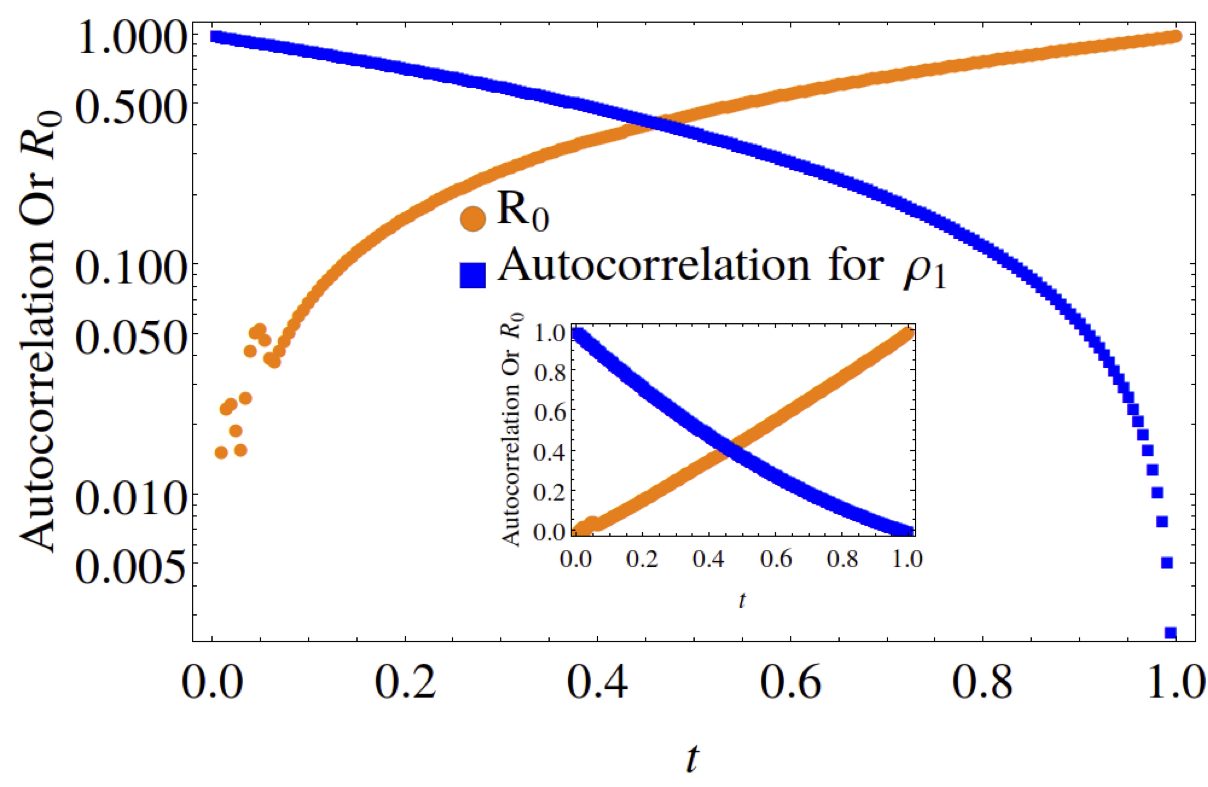
(a) Autocorrelation and $R_{0}$ of $\rho_{1}$ at $x=0.2$

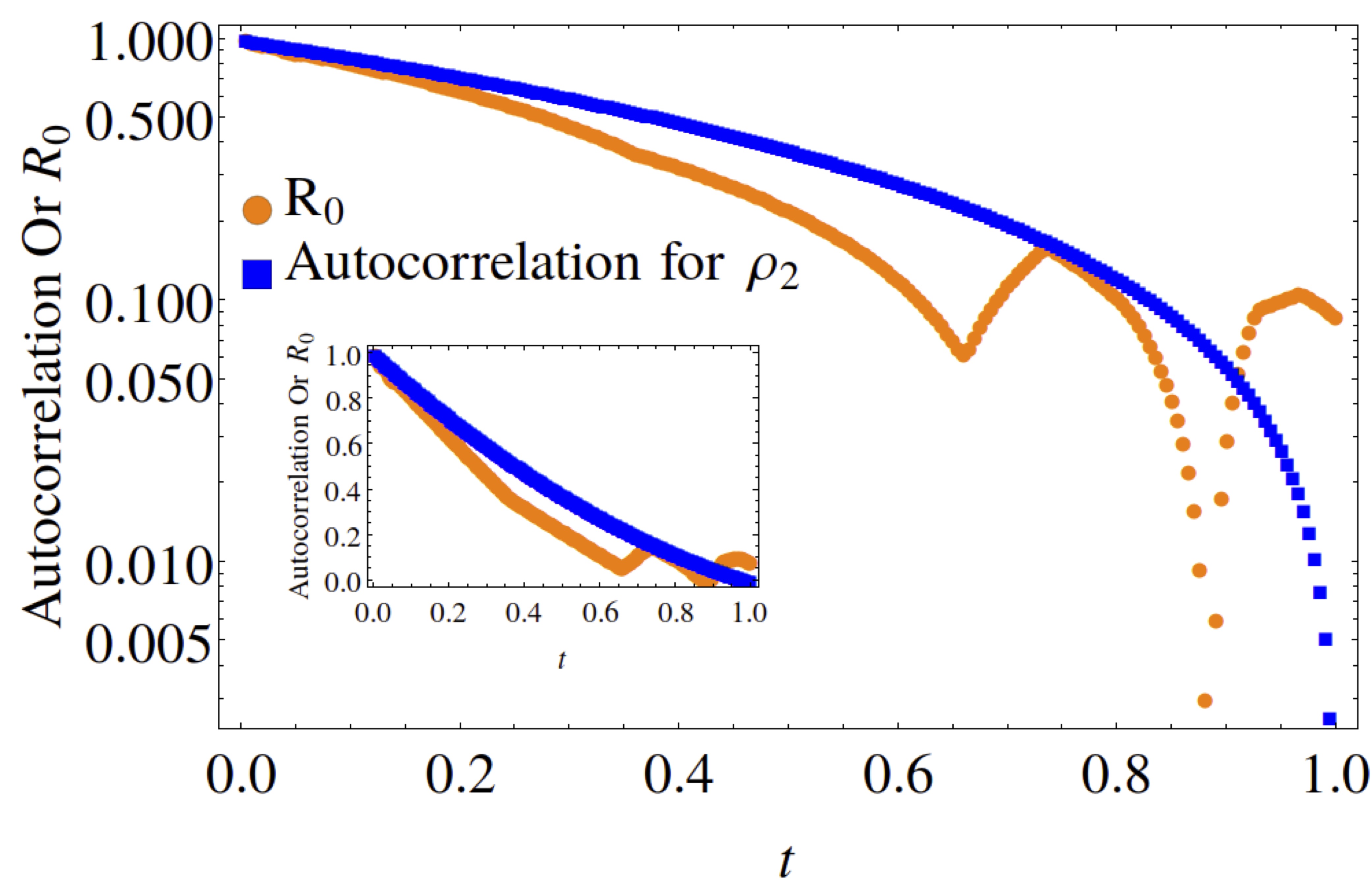
(b) Autocorrelation and $R_{0}$ of $\rho_{2}$ at $x=0.2$

Figure 1: Comparison of normalized autocorrelation and $R_{0}$ at $x=0.2$. Outset is in log scale and inset is in original scale. Panel (a) shows that the autocorrelation (in blue) is decreasing at later times although the $R_{0}$ is increasing for the species $\rho_{1}$ (orange curve). This indicates that at $x=0.2$ the production of $\rho_{1}$ occurs from its own population at small timescales. On the other hand, in panel (b), the simultaneous decreasing behavior of the autocorrelation and $R_{0}$ indicate that at $x=0.2$ the production of $\rho_{2}$ also occurs at smaller timescales. However, in case of $\rho_{2}$, its production occurs due to the conversion of $\rho_{1}$ into $\rho_{2}$, since the measure of self-creation $R_{0}$ is decreasing in this case.

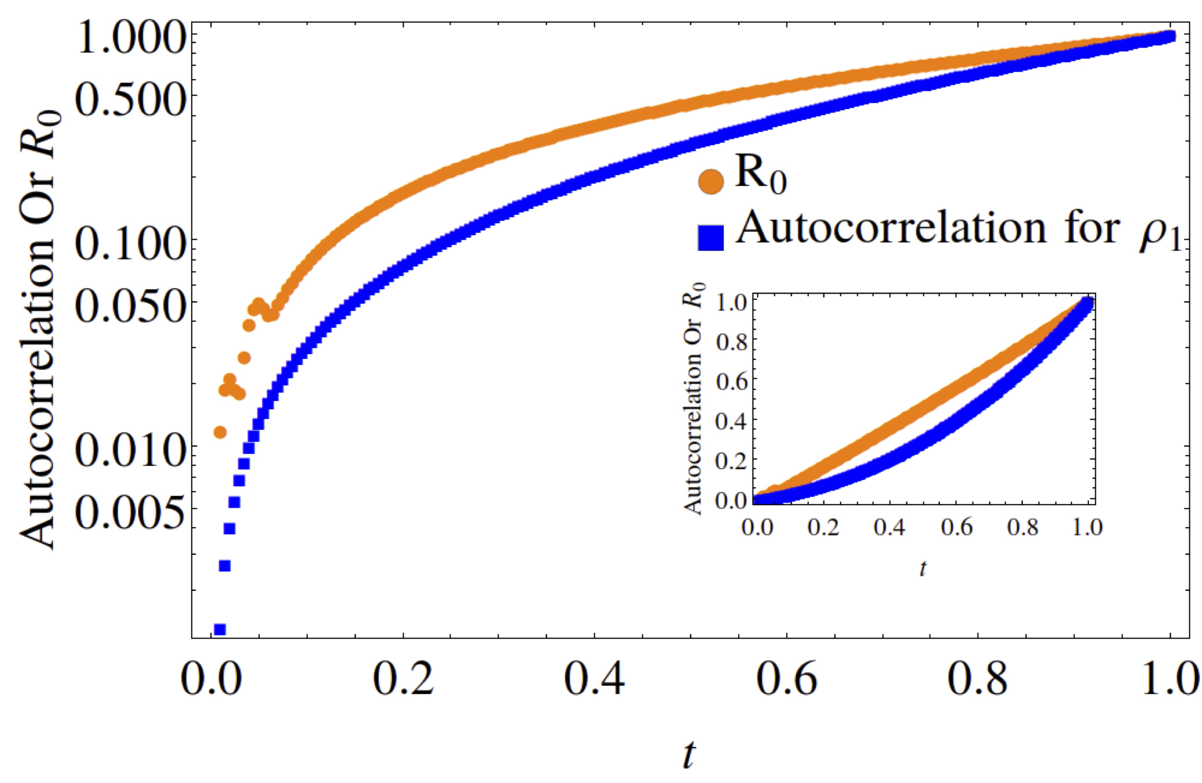
(a) Autocorrelation and $R_{0}$ of $\rho_{1}$ at $x=0.3$

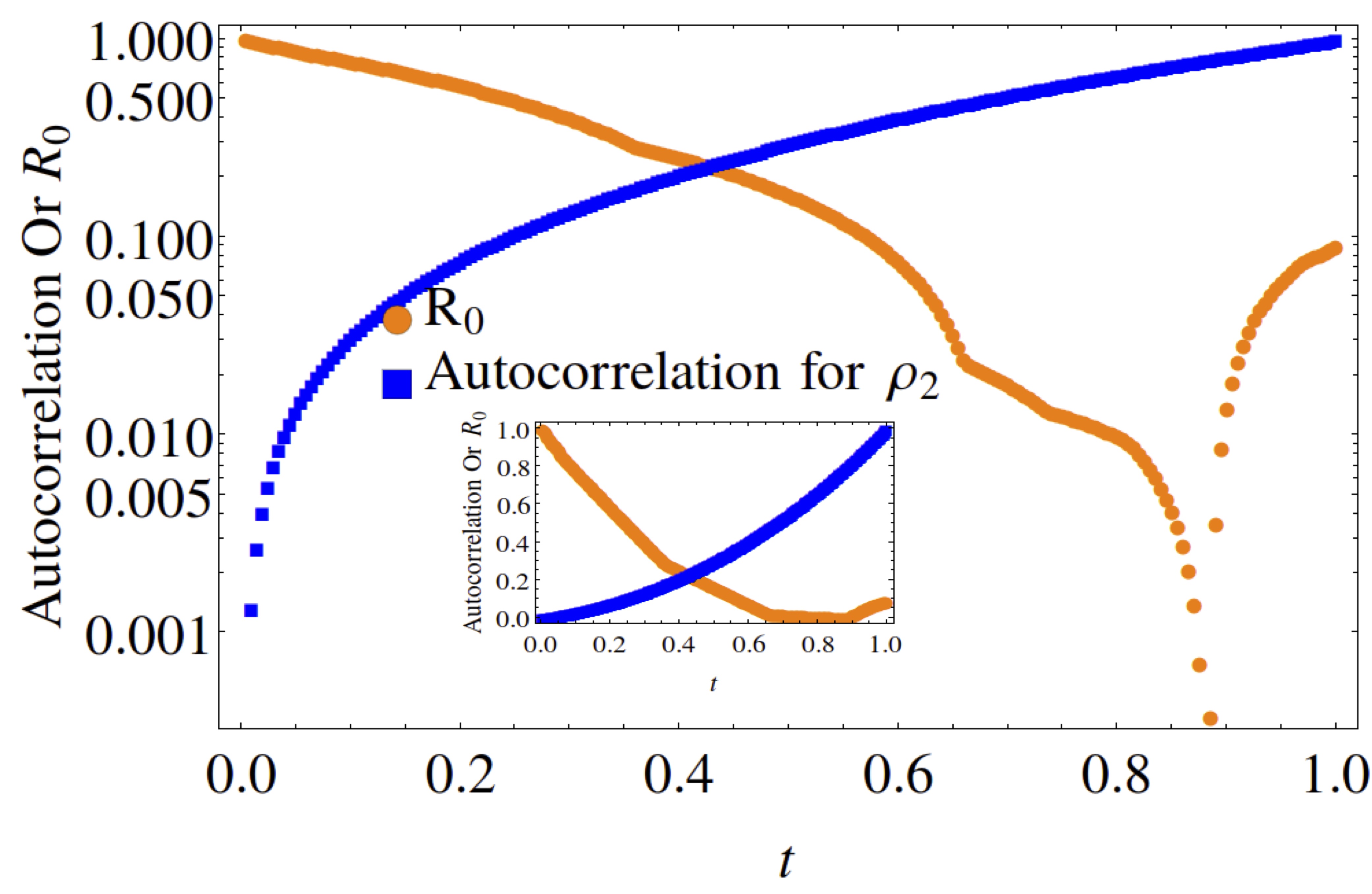
(b) Autocorrelation and $R_{0}$ of $\rho_{2}$ at $x=0.3$

Figure 2: Comparison of normalized autocorrelation and $R_{0}$ at $x=0.3$. Outset is in log scale and inset is in original scale. Panel (a) shows that the autocorrelation function and $R_{0}$ for the species $\rho_{1}$ have the same increasing trend as a function of time. The understanding we get from this trend is that the species $\rho_{1}$ is produced fom its own species for long time-scales. Panel (b) indicates that the dynamics of the species $\rho_{2}$ is quite different than $\rho_{1}$. The species $\rho_{2}$ is produced from the conversion of $\rho_{1}$ instead from its own ancestors, as the $R_{0}$ for $\rho_{2}$ decreases over time.

Figures 1, 2, 3, 4 compare the $R_{0}$ equivalent of an equivalent epidemic rate model with that of the autocorrelation function (Eqn. (2a,2b) at the quantitative level, providing interesting insights into the D-D reaction-diffusion model. It can be easily understood from the mathematical expression of $R_{0}(t)$ that it is a measure of the production rate of a species from the population of the same species at an earlier epoch, rather than due the conversion of other species. On the other hand, autocorrelation is a measure of the abundance of a species as a whole, aggregating the production of a species from it’s own population as well as due to the conversion of other species. Therefore, the autocorrelation function together with the time-varying $R_{0}(t)$, gives us interesting spatio-temporal insights about the observed abundance

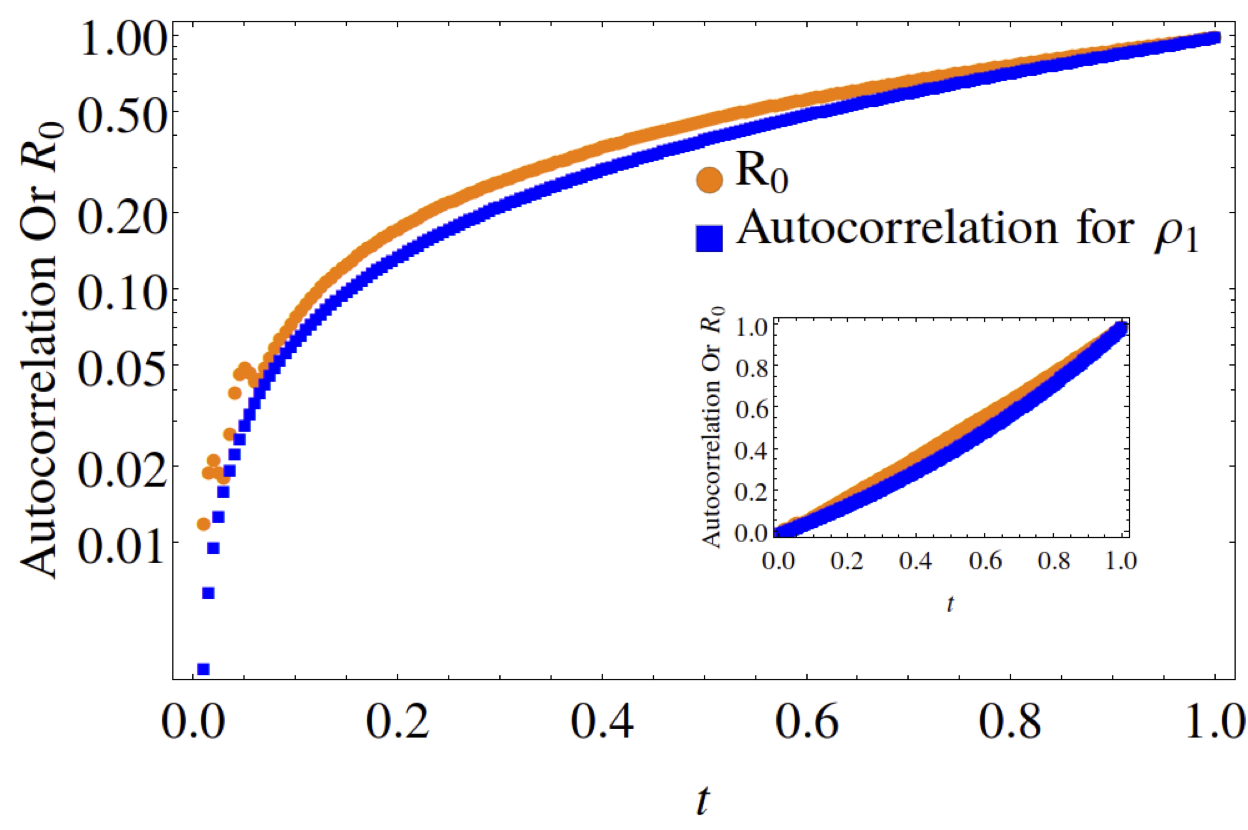
(a) Autocorrelation and $R_{0}$ of $\rho_{1}$ at $x=0.5$

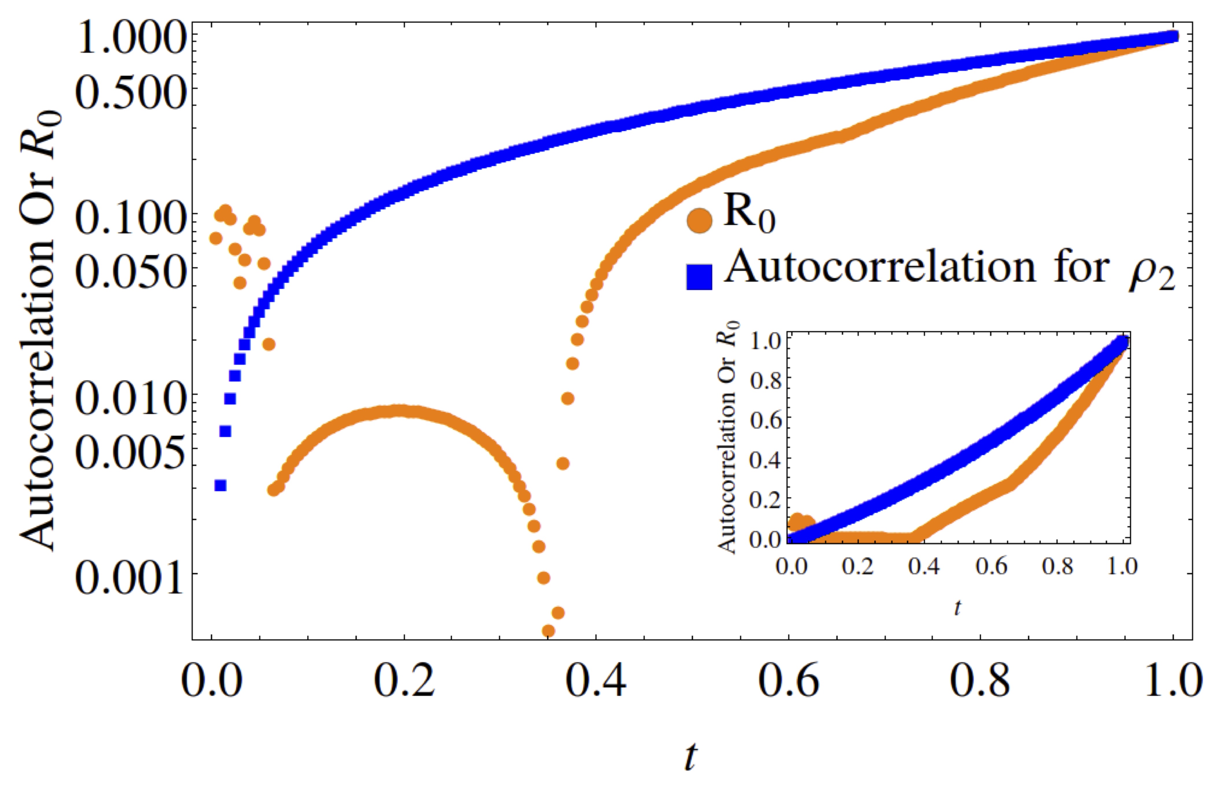
(b) Autocorrelation and $R_{0}$ of $\rho_{2}$ at $x=0.5$

Figure 3: Comparison of normalized autocorrelation and $R_{0}$ at $x=0.5$. Outset is in log scale and inset is in original scale. Panel (a) shows similar trend for $R_{0}$ and autocorrelation as in Fig.2(a), which indicates that the production of $\rho_{1}$ is boosted by the abundance of its ancestor. Whereas, the production of $\rho_{2}$ occurs both by the conversion of $\rho_{1}$ for some time and due to its own population at later times.

A comparison between Figures 1 and 2 with 3 clearly indicates that while asymmetric cases ($x<0.5$) ensure only partial convergence between the $R_{0}$ and autocorrelation profiles, i. e. only one of the two double diffusing variables match both profiles, at $x=0.5$, the profiles match (approximately) for both variables.

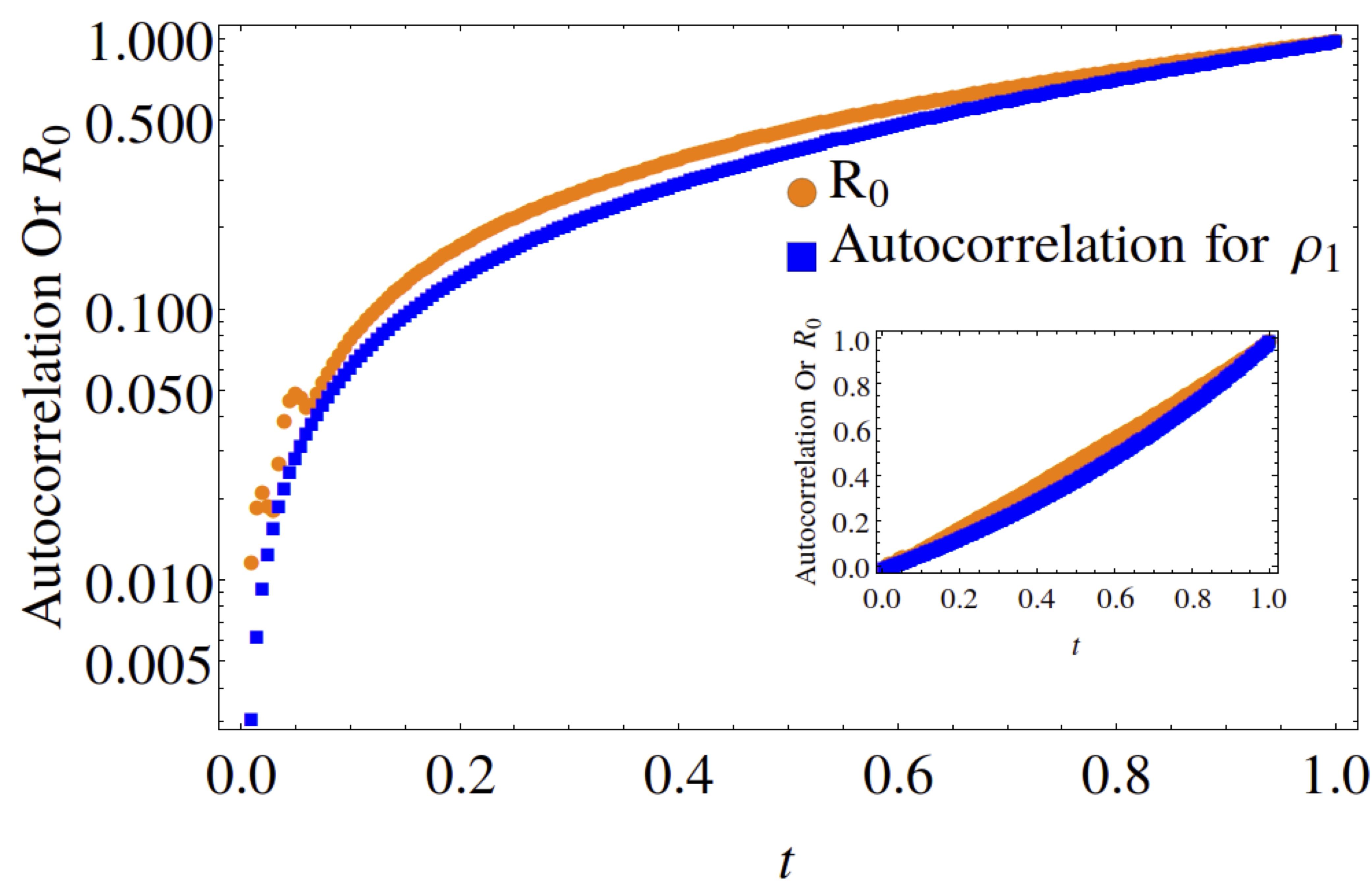
(a) Autocorrelation and $R_{0}$ of $\rho_{1}$ at $x=0.6$

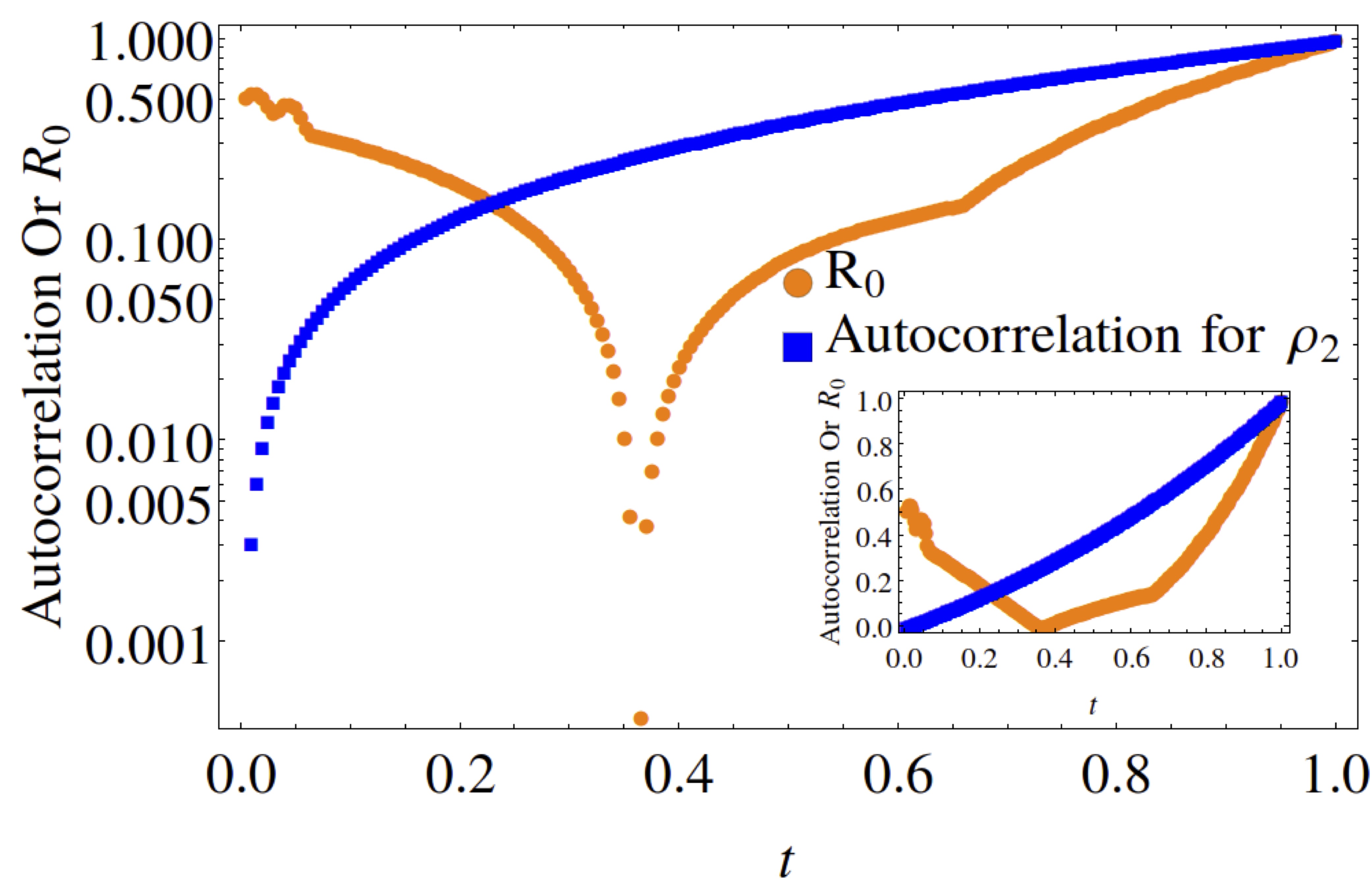
(b) Autocorrelation and $R_{0}$ of $\rho_{2}$ at $x=0.6$

Figure 4: Comparison of normalized autocorrelation and $R_{0}$ at $x=0.6$. Outset is in log scale and inset is in original scale. The dynamics at $x=0.6$ is almost similar to that of at $x=0.5$, as shown in Fig.3.

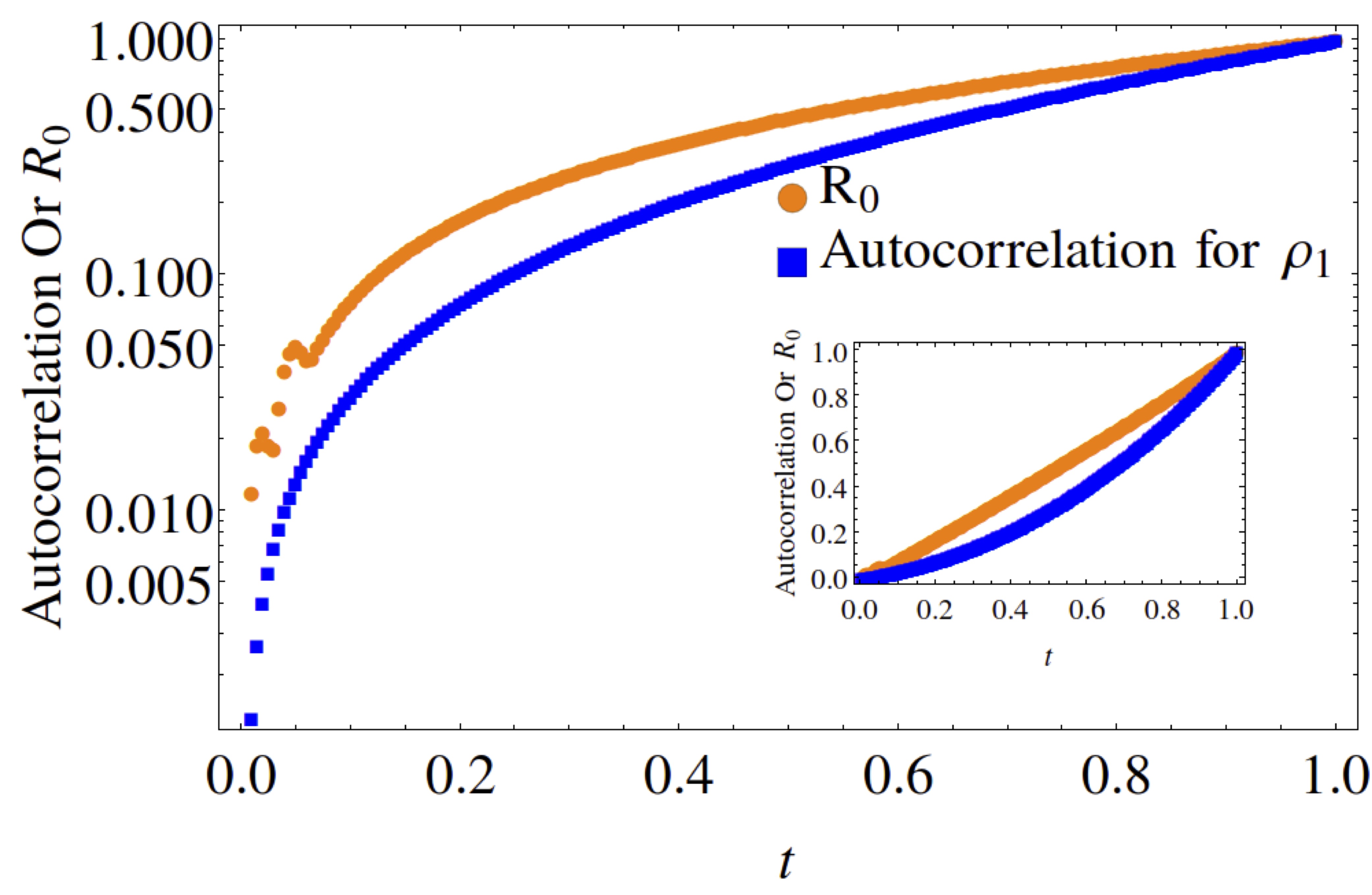
(a) Autocorrelation and $R_{0}$ of $\rho_{1}$ at $x=0.7$

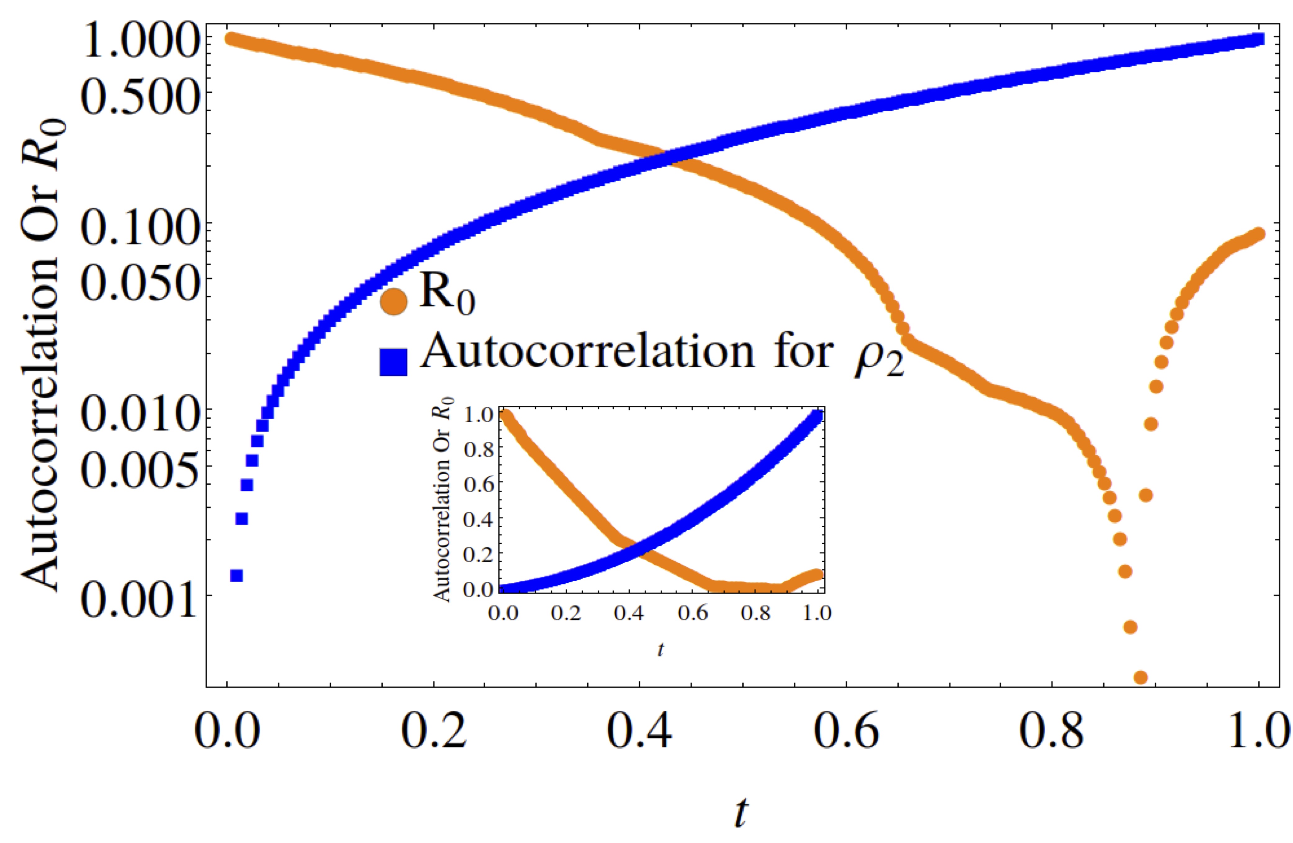
(b) Autocorrelation and $R_{0}$ of $\rho_{2}$ at $x=0.7$

Figure 5: Comparison of normalized autocorrelation and $R_{0}$ at $x=0.7$. Outset is in log scale and inset is in original scale.

Note, the dynamics of $\rho_{1}$ as shown in Figure 5 matches those for $x=0.3,0.5,0.6$. However, the species $\rho_{2}$ is mostly created by the conversion of the species $\rho_{1}$. These 5 figures clearly indicate that only for the symmetric case $x=0.5$, the time dynamical evolution of the reproductive number for an epidemic model matches the average energy dissipation rate of individual variables (expressed as autocorrelation functions), not otherwise. This is not unexpected as the point $x=0.5$ (spatial scale $0<x<1$) represents the point of dynamical equilibrium between two diffusing species, that also represents infection flux equilibrium between susceptible-infected-recovered species in an epidemic model. In other words, a fair quantitative comparison between the $R_{0}$ versus the D-D model is only ensured at $x=0.5$.

6 Conclusions

Clearly, a comparison of the dynamical variable $R_{0}(t)$, motivated by the epidemiological literature, with the autocorrelation function reveals the richness of the dynamics of a reaction-diffusion system which offers an option of interpolating the results from the epidemic model into the double-diffusion domain, in the process providing a closed form solution of the latter that has remained elusive thus far. Comparing the time evolution of $R_{0}$ with the autocorrelation function gives the information of the origin of the observed abundance of different species in a reaction-diffusion system as explained in Figures 1 to 5. The analogy is strictly restricted to the spatially symmetric ($x=0.5$) conformation though, a point of dynamical equilibrium between two (or multiple) diffusing species, an analogy with the stationary state fixed point of an epidemic model in dynamical equilibrium.

Therefore, the introduction of the epidemiologically motivated quantity $R_{0}(t)$ into the studies of the reaction-diffusion systems can play a crucial role in understanding such systems in more depth. Since this interpolation between two unrelated disciplines only uses the mathematical similarity between two (or multiple) reaction-diffusion species, expressed as double-diffusion in material science, as compared to infection rate growth in epidemiology, the approach is generic enough to be applied to all coupled reaction-diffusion models. At the point of symmetry ($x=0.5$ in our model), both quantities ($R_{0}$ and autocorrelation) will asymptotically match their values with evolving time allowing for a closed form mapped (from mathematical biology) solution of the R-D model. As a comparison with the numerical solution confirms close convergence with the approximate mapped solution (based on the $R_{0}(t)$ formula as a descriptor of the correlation strength of the diffusing variables), the solution provides handle to studies analyzing higher order perturbations and relevant bifurcations, also including stochastic terms. Future studies involving calculation of correlated superconducting fluxes would be presented using the same method.

References

- (1) D. Walgraef and E. C. Aifantis, Dislocation patterning in fatigued metals as a result of dynamical instabilities, Journal of Applied Physics 58, 688 (1985).
- (2) D. Walgraef and E. C. Aifantis, Dislocation patterning in fatigued metals: Labyrinth structures and rotational effects, nternational Journal of Engineering Science, 24(12), 1789-1798 (1986).
- (3) E. C. Aifantis, On the dynamical origin of dislocation patterns, Materials Science and Engineering 81, 563-574 (1986).
- (4) E. C. Aifantis, Gradient nanomechanics: Applications to deformation, fracture, and diffusion in nanopolycrystals, Metall. Mater. Trans. A 42, 2985 (2011).
- (5) E. C. Aifantis and J. M. Hill, On the theory of diffusion in media with double diffusivity I—Basic mathematical results, Q. J. Mech. Appl.Math. 33, 1 (1980).
- (6) E. C. Aifantis and J. M. Hill, On the theory of diffusion in media with double diffusivity II—Basic mathematical results, Q. J. Mech. Appl.Math. 33, 1 (1980).
- (7) A. K. Chattopadhyay and E. C. Aifantis, Double diffusivity model under stochastic forcing, Physical Review E 95, 052134 (2017).
- (8) A. K. Chattopadhyay and E. C. Aifantis, On stochastic resonance in a model of double diffusion, Materials Science and Technology, 34:13, 1606-1613 (2018).
- (9) A. K. Chattopadhyay and E. C. Aifantis, Stochastically forced dislocation density distribution in plastic deformation, Physical Review E 94, 022139 (2016).
- (10) I. Vardoulakis and E. C. Aifantis, A gradient flow theory of plasticity for granular materials, Acta Mechanica 87, 197–217 (1991).
- (11) J. Pontes, D. Walgraef, and E. C. Aifantis, On dislocation patterning: Multiple slip effects in the rate equation approach, Intl. J. Plasticity 22, 1486 (2006).
- (12) K. Spillotis, L. Russo and E. C. Aifantis, Analytical and numerical bifurcation analysis of dislocation pattern formation of the Walgraef–Aifantis model, International Journal of Non-Linear Mechanics 102, 41-52 (2018).
- (13) E. C. Aifantis, Gradient Extension of Classical Material Models: From Nuclear & Condensed Matter Scales to Earth & Cosmological Scales. In: Ghavanloo E., Fazelzadeh S.A., Marotti de Sciarra F. (eds) Size-Dependent Continuum Mechanics Approaches. Springer Tracts in Mechanical Engineering. Springer, Cham. https://doi.org/10.1007/978-3-030-63050-8_15
- (14) E. C. Aifantis, A new interpretation of diffusion in high-diffusivity paths—a continuum approach, Acta Metllurgica 27(4), 683-691 (1979).
- (15) , E. C. Aifantis, Comments on the calculation of the formation volume of vacancies in solids, Physical Review B 19, 6622 (1979).
- (16) E. C. Aifantis, Continuum basis for diffusion in regions with multiple diffusivity, Journal of Applied Physics 50, 1334 (1979).
- (17) R. K. Wilson and E. C. Aifantis, On the theory of consolidation with double porosity, International Journal of Engineering Science 20(9), 1009-1035 (1982).
- (18) A. -A. Tsambali, A. Konstantinidis and E. C. Aifantis, modeling double diffusion in soils and materials, Journal of the Mechanical Behavior of Materials; https://doi.org/10.1515/jmbm-2018-2003.
- (19) E. C. Aifantis, On the problem of diffusion in solids, Acta Mechanica 37—, 265-296 (1980).
- (20) J. M. Hill, A discrete random walk model for diffusion in media with double diffusivity, The ANZIAM Journal 22(1), 58 - 74 (1980).
- (21) J. M. Hill, A discrete random walk model for diffusion in media with double diffusivity, Journal of Australian Mathematical Society 22 (Series B), 58-74 (1980).
- (22) , K. Kuttler and E. C. Aifantis, Existence and uniqueness in nonclassical diffusion, Quarterly of Applied Mathematics 45(3), 549-560 (1987).
- (23) I. Santra, S. Das and S. K. Nath, Brownian motion under intermittent harmonic potentials, Journal of Physics A: Mathematical and Theoretical 54, 334001 (2021).
- (24) D. Konstantinidis, I. Eleftheriadis and E. C. Aifantis, Application of double diffusivity model to superconductors, Journal of Materials Processing Technology 108(2):185-187 (2001).
- (25) J. L. Vasquez, A de Pablo, F. Quirós and A. Rodríguez, Classical solutions and higher regularity for nonlinear fractional diffusion equations, JEMS 19(7), 1949–1975 (2017).
- (26) L. I. Rubinstein, The Stefan Problem, Translations of Mathematical Monographs 27 (2010).
- (27) M. El-Hachem, S. W. McCue, W. Jin, Y. Du and M. J. Simpson, Revisiting the Fisher–Kolmogorov–Petrovsky–Piskunov equation to interpret the spreading–extinction dichotomy, Proc. of Roy. Soc. A 275(2299); https://doi.org/10.1098/rspa.2019.0378.
- (28) J. D. Murray, Mathematical Biology (Biomathematics Series), 1994 Edition, (2nd, Corr. Ed) Publisher: Springer-Verlag New York Inc.
- (29) J. E. Pearson, Complex Patterns in a Simple System, Science 261(5118), 189-192 (1993). spiliotis2018analytical. Mathematical behavior of nonlinear Reaction-Diffusion equations and its numerical solutions have been extensively studied in conway1978large, pao1982nonlinear, pao2001numerical.
- (30) H Nishiura, Correcting the Actual Reproduction Number: A Simple Method to Estimate R0 from Early Epidemic Growth Data, International Journal of Environmental Research in Public Health 7(1): 291–302 (2010).
- (31) A Cori, N M Ferguson, C Fraser, S Cauchemez, A New Framework and Software to Estimate Time-Varying Reproduction Numbers During Epidemics, American Journal of Epidemiolgy 178(9): 1505–1512 (2013)..
- (32) A. K. Chattopadhyay, D. Choudhury, G. Ghosh, B. Kundu and S. K. Nath, Infection kinetics of Covid-19 and containment strategy, Scientific Reports volume 11, Article number: 11606 (2021).