Discovery of 74 new bright ZZ Ceti stars in the first three years of TESS

Abstract

We report the discovery of 74 new pulsating DA white dwarf stars, or ZZ Cetis, from the data obtained by the Transiting Exoplanet Survey Satellite (TESS) mission, from Sectors 1 to 39, corresponding to the first 3 cycles. This includes objects from the Southern Hemisphere (Sectors 1–13 and 27–39) and the Northern Hemisphere (Sectors 14–26), observed with 120 s- and 20 s-cadence. Our sample likely includes 13 low-mass and one extremely low-mass white dwarf candidate, considering the mass determinations from fitting Gaia magnitudes and parallax. In addition, we present follow-up time series photometry from ground-based telescopes for 11 objects, which allowed us to detect a larger number of periods. For each object, we analysed the period spectra and performed an asteroseismological analysis, and we estimate the structure parameters of the sample, i.e., stellar mass, effective temperature and hydrogen envelope mass. We estimate a mean asteroseismological mass of $\langle M_{\rm sis}\rangle$= 0.635$\pm$ 0.015 M_⊙, excluding the candidate low or extremely-low mass objects. This value is in agreement with the mean mass using estimates from Gaia data, which is $\langle M_{\rm phot}\rangle$= 0.631$\pm$ 0.040 M_⊙, and with the mean mass of previously known ZZ Cetis of $\langle M_{*}\rangle$= 0.644 $\pm$ 0.034 M_⊙. Our sample of 74 new bright ZZ Cetis increases the number of known ZZ Cetis by $\sim$20 per cent.

1 Introduction

Variable DA white dwarf or ZZ Ceti stars are cool pulsating white dwarfs, with an instability strip located between effective temperatures of $\sim 13\,000$ K and 10 000 K, depending on stellar mass (Hermes et al., 2017a; Kepler & Romero, 2017). These objects show photometric variations with periods between 70 and 2000 s, and amplitudes up to 0.3 mag (Winget & Kepler, 2008; Fontaine & Brassard, 2008; Althaus et al., 2010a; Córsico et al., 2019), corresponding to spheroidal non-radial gravity modes with low harmonic degree.

Depending on their effective temperature and pulsational properties, ZZ Cetis can be classified as hot, intermediate and cool ZZ Cetis (Clemens, 1993; Mukadam et al., 2006). The hot ZZ Cetis are located at the blue edge of the instability strip. They show a stable sinusoidal or sawtooth light curve, with a few modes with short periods (<350 s) and small amplitudes (1.5–20 mma). The cool ZZ Cetis, on the other hand, are located at the red edge of the instability strip, showing a collection of long periods (up to 1500 s), with large variation amplitudes (40–110 mma). Their light curves are non-sinusoidal and suffer from severe mode interference. Finally, the intermediate ZZ Cetis show mixed characteristics from hot and cool members. To date, there are roughly 420 ZZ Cetis known (see for instance Bognar & Sodor, 2016; Córsico et al., 2019; Vincent et al., 2020; Guidry et al., 2021).

The excitation mechanism acting on ZZ Ceti stars is related to an opacity bump due to partial ionization of hydrogen, called the $\kappa-\gamma$-mechanism (Dolez & Vauclair, 1981; Winget et al., 1982), which combines with the convective driving mechanism (Brickhill, 1991; Goldreich & Wu, 1999) when a thick convective region develops in the outer layers.

The Transiting Exoplanet Survey Satellite (TESS) was launched on 18 April 2018 (Ricker et al., 2014), with the primary mission of searching for exoplanets around bright target stars. Through nearly continuous stable photometry, as well as its extended sky coverage, TESS has made a significant contribution to the study of stellar pulsations in evolved compact objects (e.g. Bell et al., 2019; Wang et al., 2020; Bognár et al., 2020; Córsico et al., 2021; Uzundag et al., 2021), including variable hydrogen-rich DA white dwarf stars. The activities related to compact pulsators, as white dwarf and subdwarf stars, are coordinated by the TESS Asteroseismic Science Consortium (TASC), Compact Pulsators Working Group (WG8).

In this work we present 74 new ZZ Ceti stars discovered from the first three cycles of TESS data, from Sector 1 to Sector 39, including 120 s- and 20 s-cadence data. In addition, we perform ground-based photometry from four different telescopes for 11 objects, leading to the discovery of a new ZZ Ceti, and in most cases increasing the number of detected pulsation periods. This paper is organized as follows. We present the sample of 74 new ZZ Cetis, discovered from the TESS data in Section 2. We describe the sample selection and the data reduction for the TESS data and the ground-based observations in Section 3, including spectroscopic follow-up for 29 targets. In Section 4 we present the pulsation periods detected, and perform an asteroseismological study for our sample in Section 5. In Section 6 we present a study of the asteroseismological properties of the 74 ZZ Cetis presented in this work, and additionally one object without TESS data. We conclude in Section 7 by summarizing our findings.

2 New ZZ ceti stars

We report the discovery of 74 new bright ZZ Ceti stars from the first three years of TESS data, Sectors 1 to 39. The targets are listed in Table 1, along with the coordinates in J2000, G magnitude, effective temperature, surface gravity, and stellar mass. The parameters are taken from various works, which used different techniques to determine the effective temperature and surface gravity or stellar mass. Also included is the object TIC 20979953 which was discovered to be variable from ground based observations (see section 4.2 for details). For those objects with more than one determination for their atmospheric parameters, we include those obtained using different techniques.

To determine the atmospheric parameters, Subasavage et al. (2008) used low-resolution spectroscopy and multi-epoch $VRI$ photometry combined with near-infrared $JHK_{S}$ photometry from 2MASS. They used model atmospheres from Bergeron et al. (1995), assuming a $\log g=8.0$, because trigonometric parallaxes were not available at the time.

The atmospheric parameters from Koester et al. (2009) were based on high-resolution spectra with UVES/VLT. The spectra were compared with theoretical model atmospheres from Koester (2009).

Gianninas et al. (2011) presented the results of an spectroscopic survey of bright ($V\leq 17.5$), hydrogen-rich white dwarf stars. To derived $T_{\rm eff}$ and $\log g$ they used an updated version of the pure hydrogen model atmospheres of Liebert et al. (2005), that consider energy transport by convection following the MLT/$\alpha$ = 0.8 prescription of the mixing length theory (Tremblay et al., 2010) and improved Stark broadening profiles of hydrogen lines from Tremblay & Bergeron (2009).

Limoges et al. (2013) performed follow-up spectroscopic observations for a sub-sample of identified white dwarf stars. They employed model atmospheres described in Bergeron et al. (1995), with the improvements discussed in Tremblay & Bergeron (2009). These are pure hydrogen, plane-parallel model atmospheres, that consider energy transport by convection following the ML2/$\alpha$ = 0.7 prescription of the mixing-length theory.

Raddi et al. (2017) performed follow-up spectroscopy for a sample of white dwarfs and hot subdwarfs, extracted from an all-sky catalogue of UV, optical and IR photometry and proper motion. For the determination of the effective temperature and surface gravity for the white dwarf stars, they employed model atmospheres from Koester (2010), which adopt a MLT/$\alpha$ =  0.8 mixing length prescription for convective atmospheres and the Stark broadening computed by Tremblay & Bergeron (2009).

Most of the data presented in Table 1 were taken from Gentile Fusillo et al. (2021) and Gentile Fusillo et al. (2019), where they used the Gaia DR3 and DR2 (Gaia Collaboration et al., 2018) magnitudes and parallax, respectively, to determine the atmospheric parameters. They employed standard hydrogen atmosphere spectral models (Tremblay et al., 2011) including the $L_{\alpha}$ red wing absorption of Kowalski & Saumon (2006). To compute the stellar mass, they used the evolutionary sequences from Fontaine et al. (2001) with thick hydrogen layers and central composition C/O=50/50.

Finally, Kilic et al. (2020) and Vincent et al. (2020) rely on parallaxes from Gaia DR2 and photometry from the Sloan Digital Sky Survey (SDSS, Eisenstein et al., 2006; Kleinman et al., 2013; Kepler et al., 2019) and Panoramic Survey Telescope and Rapid Response System (Pan-STARRS, Chambers et al., 2016). They applied the photometric technique described in Bergeron et al. (1997), together with the pure hydrogen model atmospheres discussed in Bergeron et al. (2019) and reference therein. To derived $\log g$ and stellar mass they used white dwarf models similar to those described in Fontaine et al. (2001).

For some objects we determine the atmospheric parameter from the spectra we obtained with the SOAR telescope (see section 3.3 for details). We follow the fitting procedure described in detail in Kepler et al. (2019).

TIC 345202693 is in a binary system with a possible M main sequence star which has a large contribution in the infrared wavelengths, with a value for $G_{\mathrm{BP}}-G_{\mathrm{RP}}$ = 0.637 and an absolute magnitude of 11.83 from Gaia EDR3. Based on spectroscopic observations from the SOAR telescope, we estimate the effective temperature of the white dwarf component.

Table 1: List of the 74 new ZZ Ceti from TESS and TIC presented in this work. Column 1 indicates the TIC identifier. The coordinates in J2000 are in columns 3 and 4, and the G magnitude is listed in column 5. The effective temperature, $\log g$ and stellar mass determinations are listed in columns 6, 7 and 8. Data taken from the works of (1) (Gentile Fusillo et al., 2021), (2) Subasavage et al. (2008) (3) Raddi et al. (2017), (4) Koester et al. (2009), (5) Vincent et al. (2020), (6) Limoges et al. (2013), (7) Kilic et al. (2020), (8) (Gianninas et al., 2011), (9) (Kepler et al., 2019), (10) Gentile Fusillo et al. (2019) and (11) This work. The last column indicates which objects are spectroscopically confirmed DA white dwarf stars, though detection of pulsations at these temperatures implies all objects are DA white dwarfs. The object TIC 20979953 was discovered to be variable from ground-based observations

. TIC RA DEC G $T_{\rm eff}$ [K] $\log g$ Mass [$M_{\odot}$] Ref. Spectrum 5624184 09:32:48.01 $-$37:44:28.7 15.95 $11286\pm 123$ $7.588\pm 0.018$ 0.418 1 7675859 18:12:22.74 $+$43:21:07.3 16.24 $12240\pm 214$ $8.479\pm 0.023$ 0.909 1 8445665 16:24:36.81 $+$32:12:52.8 16.72 $11385\pm 235$ $7.947\pm 0.040$ 0.574 1 DA 13566624 08:51:34.85 $-$07:28:28.3 16.44 $13634\pm 298$ $8.188\pm 0.029$ 0.724 1 20979953 15:33:32.96 $-$02:06:55.7 16.53 $11859\pm 236$ $7.969\pm 0.039$ 0.587 1 $\cdots$ $\cdots$ $\cdots$ $\cdots$ $11212\pm 54$ $7.89\pm 0.01$ 0.540 7 $\cdots$ $\cdots$ $\cdots$ $\cdots$ $1132\pm 250$ $8.190\pm 0.022$ 0.713 9 DA 21187072 18:26:06.04 $+$48:29:11.3 16.28 $11808\pm 228$ $7.235\pm 0.025$ 0.314 10 DA 24603397 05:22:40.66 $-$08:02:29.7 14.71 $11832\pm 136$ $7.842\pm 0.017$ 0.517 1 DA 29862344 01:37:15.16 $-$17:27:22.7 15.25 $11613\pm 192$ $8.14\pm 0.06$ 0.682 2 DA 33717565 04:05:36.39 $-$76:28:28.1 16.52 $10675\pm 172$ $7.639\pm 0.031$ 0.433 1 DA 46847635 09:29:16.70 $-$08:40:32.2 16.75 $12018\pm 344$ $7.979\pm 0.048$ 0.593 1 55650407 04:55:27.27 $-$62:58:44.6 14.99 $11838\pm 150$ $7.945\pm 0.019$ 0.574 1 $\cdots$ $\cdots$ $\cdots$ $\cdots$ $12134\pm 67$ $7.906\pm 0.002$ 0.556 11 DA 63281499 22:28:58.15 $-$31:05:53.7 15.61 $11712\pm 166$ $7.981\pm 0.025$ 0.594 1 $\cdots$ $\cdots$ $\cdots$ $\cdots$ $12200\pm 200$ $8.02\pm 0.06$ 0.616 3 DA 65144290 07:11:14.04 $-$25:18:15.0 14.47 $11208\pm 180$ $8.12\pm 0.060$ 0.670 10 DA 72637474 02:08:07.86 $-$29:31:38.0 15.92 $10214\pm 112$ $7.209\pm 0.025$ 0.297 1 $\cdots$ $\cdots$ $\cdots$ $\cdots$ $11769\pm 250$ $7.54\pm 0.038$ 0.413 4 DA 79353860 21:18:15.52 $-$53:13:22.7 15.92 $11284\pm 196$ $7.970\pm 0.032$ 0.587 1 $\cdots$ $\cdots$ $\cdots$ $\cdots$ $11372\pm 44$ $7.982\pm 0.004$ 0.548 11 DA 116373308 03:02:11.43 $+$48:00:13.6 16.33 $12057\pm 265$ $8.043\pm 0.033$ 0.631 1 DA $\cdots$ $\cdots$ $\cdots$ $\cdots$ $11551\pm 60$ $\cdots$ 0.614 5 141976247 06:25:27.47 $-$75:40:41.7 15.58 $13121\pm 241$ $8.204\pm 0.018$ 0.733 1 DA 149863849 17:43:49.28 $-$39:08:25.9 13.53 $11604\pm 206$ $8.087\pm 0.027$ 0.657 1 DA 156064657 00:37:23.75 $-$48:21:55.9 16.60 $10193\pm 131$ $7.295\pm 0.034$ 0.320 1 DA 158068117 06:00:52.91 $-$46:30:41.1 16.09 $12719\pm 210$ $7.434\pm 0.026$ 0.376 1 167486543 04:48:32.11 $-$10:53:49.9 16.23 $12187\pm 252$ $8.547\pm 0.028$ 0.953 1 DA 188087204 10:46:27.80 $-$25:12:15.8 16.83 $10052\pm 218$ $7.583\pm 0.055$ 0.412 1 207206751 03:13:18.66 $-$56:07:35.0 14.62 $10968\pm 250$ $7.996\pm 0.038$ 0.601 10 DA 220555122 02:56:21.34 $-$63:28:40.2 15.87 $11827\pm 350$ $8.169\pm 0.045$ 0.708 1 DA 229581336 18:01:15.37 $+$72:18:49.0 16.05 $14634\pm 403$ $7.425\pm 0.035$ 0.382 1 DA $\cdots$ $\cdots$ $\cdots$ $\cdots$ $11075\pm 32$ $8.082\pm 0.022$ 0.648 11 DA 230029140 19:28:53.87 $+$61:05:48.7 16.45 $11655\pm 230$ $7.987\pm 0.051$ 0.597 1 DA 230384389 19:03:19.56 $+$60:35:52.6 15.04 $11366\pm 89$ $8.09\pm 0.014$ 0.658 10 DA 231277791 02:49:18.23 $-$53:34:35.4 16.46 $11623\pm 235$ $8.080\pm 0.035$ 0.653 1 DA 232979174 14:34:17.88 $+$65:39:59.5 16.14 $12776\pm 234$ $7.749\pm 0.025$ 0.473 1 DA 238815671 21:52:11.62 $-$63:32:36.4 16.12 $11693\pm 250$ $7.944\pm 0.038$ 0.573 10 DA 261400271 06:51:01.30 $-$80:34:09.6 14.90 $13670\pm 250$ $8.399\pm 0.038$ 0.859 10 DA 273206673 04:33:50.99 $+$48:50:39.2 15.35 $11433\pm 221$ $7.966\pm 0.035$ 0.585 1 282783760 13:14:26.82 $+$17:32:09.2 16.30 $12111\pm 268$ $8.026\pm 0.032$ 0.622 1 DA 287926830 21:50:40.62 $+$30:35:34.1 15.94 $11429\pm 79$ $\cdots$ 0.562 5 304024058 09:22:56.24 $-$68:16:48.8 16.10 $11368\pm 208$ $7.955\pm 0.033$ 0.578 1 DA 313109945 14:05:40.57 $+$74:38:59.3 15.59 $9059\pm 134$ $7.49\pm 0.04$ 0.380 1 DA 317153172 23:22:32.11 $-$83:13:14.2 16.47 $11813\pm 314$ $8.032\pm 0.042$ 0.624 1 DA 317620456 19:21:82.42 $+$27:40:25.4 15.04 $10566\pm 67$ $\cdots$ 0.603 7 $\cdots$ $\cdots$ $\cdots$ $\cdots$ $11060\pm 163$ $8.10\pm 0.05$ 0.660 6 DA 343296348 17:43:44.00 $-$74:24:37.5 15.85 $11597\pm 150$ $7.968\pm 0.023$ 0.586 1 DA 344130696 18:37:08.31 $-$76:59:05.9 15.39 $10829\pm 116$ $7.177\pm 0.018$ 0.293 1 DA 345202693 18:48:28.03 $-$74:27:60.0 16.56 $11332\pm 250$ $\cdots$ $\cdots$ 1 DA+IR 353727306 02:40:29.66 $+$66:36:37.1 15.60 $11874\pm 250$ $8.019\pm 0.038$ 0.617 10 DA 370239521 21:50:24.19 $-$53:58:37.2 14.65 $11191\pm 978$ $8.23\pm 0.44$ 0.733 11 DA+M 380298520 20:13:43.26 $+$34:13:56.0 15.68 $11834\pm 170$ $8.405\pm 0.021$ 0.861 1 DA $\cdots$ $\cdots$ $\cdots$ $\cdots$ $11440\pm 118$ $\cdots$ 0.854 5 394015496 21:58:23.88 $-$58:53:53.8 15.81 $11639\pm 141$ $8.004\pm 0.022$ 0.607 1 DA 415337224 03:54:54.26 $+$07:46:06.3 16.54 $16380\pm 308$ $7.87\pm 0.06$ 0.55 8 $\cdots$ $\cdots$ $\cdots$ $\cdots$ $10600\pm 300$ $\cdots$ 0.563 10 DA 428670887 11:58:40.65 $-$20:29:51.2 16.01 $11826\pm 175$ $8.062\pm 0.026$ 0.642 1 DA

Table 2: continued

TIC	RA	DEC	G	$T_{\rm eff}$ [K]	$\log g$	Mass [$M_{\odot}$]	Ref.	Spectrum
441500792	03:06:48.35	$-$17:23:32:9	16.68	$11393\pm 273$	$8.046\pm 0.046$	0.632	1
442962289	05:25:47.64	$-$17:33:49.9	16.51	$11945\pm 252$	$8.416\pm 0.031$	0.868	1
610337553	00:55:46.72	$-$15:04:52.7	17.36	$10680\pm 380$	$7.854\pm 0.089$	0.520	1
631161222	01:26:24.73	$-$71:17:12.0	16.96	$11435\pm 362$	$7.934\pm 0.059$	0.566	1
631344957	02:13:28.27	$-$64:37:08.9	16.98	$11574\pm 311$	$7.995\pm 0.050$	0.602	1
632543879	02:28:23.39	$+$13:47:27.3	16.98	$11850\pm 380$	$8.036\pm 0.055$	0.626	1
651462582	03:07:33.09	$-$46:53:16.3	17.08	$11210\pm 340$	$7.930\pm 0.064$	0.564	1
661119673	04:42:58.31	$+$32:37:15.6	17.37	$10668\pm 345$	$7.881\pm 0.082$	0.535	1
685410570	05:00:11.50	$-$50:46:12.4	17.04	$11257\pm 335$	$7.944\pm 0.059$	0.572	1
686044219	04:21:48.96	$-$35:58:49.8	17.13	$11477\pm 356$	$8.019\pm 0.058$	0.615	1
712406809	06:39:17.24	$+$01:13:29.5	16.22	$10669\pm 298$	$7.914\pm 0.065$	0.553	7	DA
724128806	05:37:24.22	$-$80:45:49.7	17.48	$9776\pm 239$	$7.595\pm 0.065$	0.415	1
733030384	05:32:03.91	$-$65:36:09.9	16.89	$12059\pm 193$	$8.001\pm 0.028$	0.606	1
800153845	08:55:07.25	$+$06:35:40.0	16.656	$10501\pm 273$	$7.902\pm 0.070$	0.546	1
$\cdots$	$\cdots$	$\cdots$	$\cdots$	$11119\pm 46$	$8.365\pm 0.030$	0.820	9	DA
804835539	08:54:57.51	$-$76:46:21.9	16.906	$15296\pm 476$	$8.078\pm 0.046$	0.659	1
804899734	08:32:58.10	$-$76:01:05.9	17.40	$11585\pm 305$	$7.988\pm 0.053$	0.598	1
951016050	12:14:11.95	$-$34:58:45.9	17.03	$11292\pm 263$	$7.974\pm 0.051$	0.589	1
1001545355	14:13:53.96	$+$71:36:12.6	16.99	$11244\pm 232$	$7.653\pm 0.036$	0.439	1
1102242692	15:28:09.16	$+$55:39:16.1	17.09	$10343\pm 223$	$7.459\pm 0.051$	0.372	1
$\cdots$	$\cdots$	$\cdots$	$\cdots$	$11180\pm 184$	$7.86\pm 0.07$	0.530	8	DA
1102346472	14:53:23.52	$+$59:50:56.2	17.16	$12102\pm 345$	$8.067\pm 0.045$	0.646	1
$\cdots$	$\cdots$	$\cdots$	$\cdots$	$11217\pm 250$	$7.97\pm 0.038$	0.589	9	DA
1108505075	15:44:55.68	$-$69:09:10.4	16.993	$11369\pm 225$	$7.918\pm 0.043$	0.557	1
1173423962	14:41:14.41	$-$38:46:29.7	17.38	$10719\pm 414$	$7.920\pm 0.093$	0.556	1
1201194272	16:33:58.75	$+$59:12:06.6	17.13	$11705\pm 416$	$8.018\pm 0.063$	0.616	1
1309155088	16:54:26.50	$+$23:52:41.5	16.99	$11487\pm 273$	$8.109\pm 0.045$	0.670	1
$\cdots$	$\cdots$	$\cdots$	$\cdots$	$10700\pm 91$	$8.033\pm 0.013$	0.622	7	DA
1989258883	20:14:39.52	$-$56:55:01.7	16.62	$11172\pm 188$	$7.983\pm 0.037$	0.594	1	DA
1989866634	20:43:11.73	$-$46:10:48.5	17.38	$11503\pm 419$	$7.996\pm 0.075$	0.602	1	DA
2026445610	21:24:21.14	$-$63:10:12.4	17.27	$11737\pm 274$	$8.037\pm 0.046$	0.627	1
2055504010	22:45:54.79	$-$45:00:58.9	16.84	$11050\pm 239$	$7.900\pm 0.049$	0.546	1

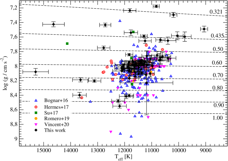
Figure 1: Distribution of ZZ Ceti stars on the $T_{\rm eff}-\log g$ plane. The coloured symbols correspond to known ZZ Ceti stars, taken from Bognar & Sodor (2016) (blue up-triangle), Hermes et al. (2017a) (red circle), Su et al. (2017) (green square), Romero et al. (2019b) (orange circle) and Vincent et al. (2020) (magenta down-triangle). The objects observed in this work are depicted with black circles. We include evolutionary tracks (dashed lines) with stellar masses between 0.435 M_⊙ and 0.9 M_⊙ from Romero et al. (2019a) and 0.321 M_⊙ from Istrate et al. (2014).

The location of the 74 new ZZ Ceti stars in the $T_{\rm eff}-\log g$ plane is presented in Figure 1. For the targets with more than one determination for the atmospheric parameters in Table 1, we adopt that obtained from photometry and parallax from Gaia for Figure 1. The sample of ZZ Ceti stars known to date is depicted in this figure, and was extracted from the works of Bognar & Sodor (2016); Hermes et al. (2017a); Su et al. (2017); Romero et al. (2019b); Vincent et al. (2020). The values for effective temperature and surface gravity derived from spectroscopy were corrected by 3D convection (Tremblay et al., 2013) for all objects (Córsico et al., 2019). Most of the objects from our sample lay around the 0.6 M_⊙ track, showing canonical masses. Note that there are 13 objects with stellar masses in the range of 0.30 $\leq$ M/M${}_{\odot}\leq$ 0.45, which correspond to low-mass white dwarfs (Kilic et al., 2007; Istrate et al., 2016; Pelisoli & Vos, 2019) and can harbour either a He/C/O- or a He-core, depending on the evolution of the progenitor star (Romero et al., 2021). TIC 345202693 has a photometric stellar mass below 0.3 M_⊙, and is a possible extremely low-mass (ELM) white dwarf variable. Finally, there are three objects with masses above 0.8 M_⊙; TIC 7675859 is the most massive object of our sample, with a photometrically determined mass of 0.909 M_⊙.

3 Observations and Data reduction

We selected the targets for the sample of DA white dwarf stars from Gentile Fusillo et al. (2019) with G $\leq$ 17.5 mag that were targeted by the TESS satellite in Sectors 1–39, with 120 s and/or 20 s-cadence. This includes both the southern (Sectors 1–13) and the northern (Sectors 14–26) hemispheres, with 120 s cadence. From Sector 27 onward, the satellite turned back to the Southern Hemisphere, and data with 20 s cadence became available for a subset of objects. In addition, we performed photometric observations from ground based telescopes with a cadence smaller than 45 s for a small subset (11) to confirm variability and to look for new periodicities. Finally, we performed spectroscopic observations for another subset (29). These data were used to improve the determination of the atmospheric parameters for some targets, and in all cases to confirm that our targets are spectroscopically confirmed DA white dwarfs. A detail description of the observations and data analysis is presented in the sections below.

3.1 TESS data

We downloaded all 2-min- and 20-s-cadence light curves of over 8 300 known white dwarfs and white dwarf candidates (Gentile Fusillo et al., 2019, 2021) brighter than G $\leq$ 17.5 mag from The Mikulski Archive for Space Telescopes, which is hosted by the Space Telescope Science Institute (STScI) in FITS format. The data were processed based on the Pre-Search Data Conditioning pipeline (Jenkins et al., 2016). We extracted times and fluxes (PDCSAP FLUX) from the FITS files. The times are given in barycentric corrected dynamical Julian days (BJD – 2457000, corrected for leap seconds, see Eastman et al., 2010). The fluxes were converted into fractional variations from the mean, that is, differential flux $\Delta I/I$, and transformed into amplitudes in parts-per-thousand (ppt). The ppt unit corresponds to the milli-modulation amplitude (mma) unit. We sigma-clipped the data at 5$\sigma$ to remove the outliers that appear above five times the median of intensities, that is, that depart from the median by 5$\sigma$.

We calculated their Fourier transforms (FTs) and examined them for pulsations or binary signatures above the 1/1000 false-alarm probability (FAP), calculated reshuffling the data 1000 times, but maintaining the same time base, and calculating their Fourier transform, selecting the highest peak. For pre-whitening, we employed our customized tool, in which, using a nonlinear least-squares (NLLS) method, we simultaneously fit each pulsation frequency in a waveform $A_{i}\sin(\omega_{1}t+\phi)$, with $\omega=2\pi/P$, and $P$ the period. This iterative process was run starting with the highest peak until no peak appeared above the 0.1% false-alarm probability significance threshold. We analysed the concatenated light curve from different sectors, if observed. The FAP was again calculated by randomizing the observations, that is, shuffling the observations one thousand times and recalculating the FTs. We calculated the amplitude at which there was a 0.1%= 1/1000 probability of any peak being due to noise (e.g. Kepler, 1993).

Because of the large pixel scale of TESS, the flux corresponding to the white dwarf ranged from CROWDSAP=0.021–0.985, meaning the total flux from the white dwarf in the extracted aperture ranged from 2.1 per cent to 98.5 per cent. To confirm the variations are from the white dwarf, we checked all stars around 120"x120" in Gaia EDR3 for other possible variables or parallax and proper motion companions. In the rare cases where a white or blue star was found, we searched for variability in every pixel of the aperture, as these might show variability on similar timescales. None was found. All PDCSAP flux values are corrected for the crowding via the CROWDSAP value, so the reported amplitudes have been corrected for flux dilution.

The third year of the TESS mission started with Sector 27. From this sector on, besides the 2-min-cadence data, some objects were observed with 20-s cadence, increasing the frequency resolution in the Fourier transform. We analyze 20-s data for 15 out of 74 ZZ Cetis in this sample.

3.2 Ground-based photometric observations

Table 3: Journal of photometric observations from ground-based facilities. We list the target, telescope, date of observation, exposure time and total observation time, in columns 1, 2, 3, 4 and 5, respectively. The sizes of the telescopes are 1-m, 4.1-m, 1.83-m and 1.6-m, for the Konkoly observatory, SOAR, Perkins and OPD, respectively.

TIC	Telescope	Run stars (UT)	texp (s)	$\Delta$t (h)
7675859	Konkoly	2020-08-20	30	5.45
		2020-08-21	30	5.95
		2020-08-22	30	4.28
		2020-08-23	45	3.96
		2020-08-25	45	5.89
		2020-08-26	45	6.14
20979953	OPD	2020-06-14	17	3.4
		2020-11-27	10	3.36
55650407	SOAR	2020-11-26	10	3.72
232979174	Konkoly	2021-07-05	45	5.05
		2021-07-06	45	5.38
		2021-07-07	30	4.81
	Perkins	2021-08-07	10	1.78
273206673	Konkoly	2020-09-11	30	4.68
		2020-10-08	30	6.88
		2020-12-11	45	4.63
		2020-12-13	30	4.23
		2020-12-14	30	3.50
		2020-12-14	45	2.53
282783760	OPD	2021-06-14	17	3.1
304024058	SOAR	2020-12-02	10	3.46
313109945	Konkoly	2020-06-11	30	2.32
		2020-06-13	30	4.71
		2020-07-04	30	4.49
		2020-07-05	30	5.18
		2020-07-07	30	4.87
370239521	OPD	2020-06-14	17	3.4
		2020-11-27	10	3.36
1989866634	OPD	2021-05-09	40	3.1
		2021-06-12	40	3.38
2055504010	OPD	2021-06-13	20	2.6
		2021-06-14	20	3.2

Ground-based follow-up photometry was performed for 11 objects with four different telescopes: the 1 m at Konkoly Observatory in Hungary, the 1.6 m Pekin-Elmer telescope at the Pico do Dias Observatory in Brazil, the 1.83-m Perkins telescope in the United States, and the 4.1 m SOAR telescope in Chile. The journal of time-series photometric observations is presented in Table 3.

For four objects, we performed observations with the 1 m Ritchey–Chrétien–Coudé telescope located at the Piszkéstető mountain station of Konkoly Observatory, Hungary. We obtained data with a Spectral Instruments 1100S CCD camera in white light. The exposure times were selected to be either 30 or 45 s. We reduced the raw data frames the standard way utilizing IRAF tasks: we performed bias and flat field corrections before the aperture photometry of field stars. We fitted low-order polynomials to the resulting light curves, correcting for long-period instrumental and atmospheric trends, and finally, we converted the observational times of every data point to barycentric Julian dates in barycentric dynamical time (BJD_TDB) using the applet of Eastman et al. (2010).

In addition, we employed Goodman image mode on the 4.1-m Southern Astrophysical Research (SOAR) Telescope in Chile. We used read out mode 200 Hz ATTN2 with the CCD binned $2\times 2$, with a ROI reduced to 800$\times$800. All observations were obtained with a red blocking filter S8612. The integration times varied from 10 to 15 s, depending on the magnitude of the object and the weather conditions. Note that with this configuration, the read-out time is $\sim 5$ s.

Five objects were observed using the IxON camera on the 1.6-m Perkin Elmer Telescope at the Pico dos Dias Observatory, in Brazil. We used a red blocking filter BG40. The integration times varies from 20 to 45 s, depending on the magnitude of the object, with a read-out time of less than 1 s.

For one object we obtained a light curve using the Perkins Re-Imaging SysteM (PRISM) mounted on the 1.8m Perkins Telescope Observatory (PTO) on Anderson Mesa outside of Flagstaff, Arizona. We used a red-cutoff BG40 filter with 10-s exposures, minimizing readouts by windowing the CCD to 410 $\times$ 380 pixels.

We reduced the data with the software IRAF, and perform aperture photometry with DAOFOT. We extracted light curves of all bright stars that were observed simultaneously in the field. Then, we divided the light curve of the target star by the light curves of all comparison stars to minimize effects of sky and transparency fluctuations. To look for periodicities in the light curves, we calculate the Fourier transform (FT) using the software PERIOD04 (Lenz & Breger, 2004). We accepted a frequency peak as significant if its amplitude exceeds the 0.1% FAP. We then use the process of pre-whitening the light curve by subtracting out of the data a sinusoid with the same frequency, amplitude, and phase of the highest peak, and then computing the FT for the residuals. We redo this process until we have no new significant signals.

3.3 Ground-based spectroscopic observations

To confirm they are DA white dwarfs and to improve the determinations of the atmospheric parameters, we obtained follow-up spectroscopic observations for 29 objects from our new ZZ Ceti stars sample. Many of these observations were organized through Working Group 8 on compact objects of the TESS Asteroseismic Consortium and are detailed in Table LABEL:tablespectroscopy.

Table 4: Log of spectroscopic observations.

TIC	UT Date	Grating	Exp.	Telescope/Inst.
		(l mm-1)	(sec)
21187072	2021-03-23	300	1200	LDT/DEVENY
24603397	2021-09-21	930	900	SOAR/GOODMAN
29862344	2019-06-17	930	1500	SOAR/GOODMAN
$\cdots$	2021-10-11	930	900	SOAR/GOODMAN
33717565	2021-09-21	930	3000	SOAR/GOODMAN
55650407	2019-12-05	930	1620	SOAR/GOODMAN
$\cdots$	2020-12-07	400	720	SOAR/GOODMAN
63281499	2019-08-22	600	600	DUPONT/B&C
$\cdots$	2019-12-05	930	1080	SOAR/GOODMAN
65144290	2021-03-05	400	400	SOAR/GOODMAN
$\cdots$	2021-09-21	930	600	SOAR/GOODMAN
79353860	2018-06-02	930	1080	SOAR/GOODMAN
$\cdots$	2021-09-21	400	1800	SOAR/GOODMAN
116373308	2020-10-19	300	840	LDT/DEVENY
149863849	2021-09-21	930	900	SOAR/GOODMAN
156064657	2021-09-21	930	2400	SOAR/GOODMAN
167486543	2021-10-12	400	540	SOAR/GOODMAN
207206751	2021-03-05	400	900	SOAR/GOODMAN
$\cdots$	2021-09-21	930	1200	SOAR/GOODMAN
220555122	2021-03-05	400	1200	SOAR/GOODMAN
$\cdots$	2021-09-21	930	2400	SOAR/GOODMAN
229581336	2021-03-23	300	1920	LDT/DEVENY
230029140	2021-03-23	300	540	LDT/DEVENY
231277791	2021-09-21	930	2400	SOAR/GOODMAN
232979174	2021-03-23	300	900	LDT/DEVENY
238815671	2019-06-17	930	3000	SOAR/GOODMAN
$\cdots$	2021-06-19	400	500	SOAR/GOODMAN
261400271	2021-03-05	400	500	SOAR/GOODMAN
304024058	2019-12-05	930	1440	SOAR/GOODMAN
343296348	2019-08-18	930	720	SOAR/GOODMAN
344130696	2019-08-18	930	1440	SOAR/GOODMAN
$\cdots$	2021-10-11	930	900	SOAR/GOODMAN
353727306	2020-09-22	300	1500	LDT/DEVENY
370239521	2019-06-17	930	540	SOAR/GOODMAN
$\cdots$	2021-06-19	400	350	SOAR/GOODMAN
380298520	2020-09-22	300	1200	LDT/DEVENY
394015496	2018-08-31	930	900	SOAR/GOODMAN
$\cdots$	2021-06-19	400	500	SOAR/GOODMAN
428670887	2021-06-18	400	1200	SOAR/GOODMAN
1989258883	2021-06-19	400	900	SOAR/GOODMAN

One ZZ Ceti, TIC 63281499, was observed with the Boller and Chivens (B&C) spectrograph mounted at the 2.5-meter (100-inch) Iréne du Pont telescope at Las Campanas Observatory in Chile. The B&C spectra were obtained using the 600 lines/mm grating corresponding to the central wavelength of 5000 Å, and covering a wavelength range from 3427 to 6573 Å. We used a 1 arcsec slit, which provided a resolution of 3.1 Å. The data from Dupont@B&C was reduced and analysed using PyRAF (Science Software Branch at STScI, 2012) procedures with the following way: First, bias correction and flat-field correction have been applied. Then, the pixel-to-pixel sensitivity variations were removed by dividing each pixel with the response function. After this reduction was completed, we have applied wavelength calibrations using the frames obtained with the internal HeAr comparison lamp. In a last step, flux calibrations were applied using the standard star EG 274. The signal-to-noise ratio (SNR) of the final spectra is around 65 (see Table LABEL:tablespectroscopy).

Additionally, seven new ZZ Cetis were observed with the DeVeny Spectrograph mounted on the 4.3-m Lowell Discovery Telescope (DT Bida et al., 2014) in Happy Hack, Arizona, United States. Using a 300 line 1/mm grating we obtain a roughly 4.5 resolution. Our spectra were debiased and flat-fielded using standard STARLINK routines (Currie et al., 2014), were optimally extracted (Horne, 1986) using the software PAMELA, and were wavelength-calibration (including a heliocentric correction) using MOLLY (Marsh, 1989).

The majority of our southern spectroscopic observations have been obtained using the Southern Astrophysical Research (SOAR) Telescope and the Goodman spectrograph (Clemens et al., 2004), situated at Cerro Pachón, Chile. We use two main setups: in our lower-resolution setup, we use the 400 l/mm grating with the blaze wavelength 5500 Å (M1: 3000-7050 Å) with a slit of 1 arcsec. This setup provides a resolution of about 5 Å. Most commonly, we used the 930 l/mm grating (M2: 3850-5550 Å) with a slit of 0.46 arcsec. This setup provides a resolution of about 2 Å. Table LABEL:tablespectroscopy outlines which grating was used for each object. The data reduction has been partially done by using the instrument pipeline including overscan, trim, slit trim, bias and flat corrections. For cosmic rays identification and removal, we used an algorithm as described by Pych (2004), which is embedded in the pipeline. The extraction and calibration of the spectra were carried out similarly as for Dupont@B&C using standard PyRAF tasks.

4 Periods and data analysis

In this section we present the results from the light curve analysis of the 74 new bright ZZ Ceti stars. The values of the detected periods are listed in Table 5 for the results based on TESS data. We also include the corresponding sectors and the amplitude detection limit for false-alarm probability FAP=1/1000. Figure 2 shows the Fourier transform (top panel) and the complete light curve (bottom panel) for the object TIC 313109945. This object shows seven peaks above the FAP=1/1000 confidence level, depicted as a red line. A long period of 6.60 d is also present at low frequencies.

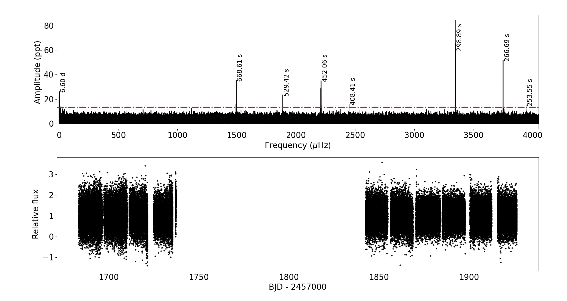
Figure 2: Fourier transform for TIC 313109945, for data with 120 s cadence corresponding to Sectors 14, 15, 20 and 21. The horizontal red line corresponds to the false-alarm probability FAP=1/1000 detection limit for the combined data.

Table 5: Detected periods for the new ZZ Cetis from TESS. For each object we list the sectors where the target was observed by the TESS satellite, indicating the 20 s cadence runs with "f” (col 2), the value of the amplitude detection limit for false-alarm probability FAP(1/1000) (col 3), and the list of periods compatible with stellar pulsations in white dwarfs (col 4). We truncate all periods to two decimals places only because the uncertainties in the theoretical models are of the order of 1 s.

TIC	sector	FAP(1/1000) [ppt]	$\Pi$ [s] (A [ppt])
5624184	f35-f36	4.58	503.99s (6.28), 445.92 (4.77), 431.31 (4.66)
7675859	25,26	9.38	353.25 (27.39), 356,09 (14.32), 360.32 (9.33), 798.66 (12.08), 743.44 (11.09)
8445665	24,25	8.78	812.76 (18.20), 638.22 (15.05), 1018.48 (8.97), 578.05 (8.92), 356.87 (8.84)
13566624	34	7.01	421.87 (8.92), 407.63 (7.83)
21187072	25,26	3.63	1076.86 (6.79), 1074.27 (4.99), 1070.74 (3.92)
24603397	5,32	1.94	262.65 (3.13)
29862344	03,f30	2.67	737.57 (3.37), 857.43 (4.03), 898.93 (2.74), 352.09 (2.22)
33717565	27-29,32,35-36,39	3.58	364.92 (10.33), 526.98 (4.47)
46847635	35	8.84	415.81 (9.66)
55650407	11-13,f27-f39	0.48	320.76 (1.65), 262.46 (7.21), 200.08 (4.42), 126.84 (1.84)
63281499	01,f28	2.94	320.52 (8.542), 383.70 (2.93)
65144290	7,33-34	4.87	278.172 (7.272)
72637474	03,f30	2.51	901.16 (2.69), 814.44 (2.56), 966.24 (2.55)
79353860	1,27	3.46	945.19 (4.29), 842.43 (3.50), 525.56 (3.60)
116373308	18	40.82	361.81 (59.30)
141976247	1-8,10-13,27-34,f35-f37	0.71	261.72 (0.86)
149863849	f39	1.78	397.98 (6.90), 397.04 (6.43), 491.21 (7.45), 568.09 (3.14), 487.36 (3.07)
156064657	29	6.04	1418.05 (13.45), 1546.56 (6.05)
158068117	5-7,32-33	1.98	268.45 (2.48)
167486543	f32	6.27	535.26 (19.83), 534.59 (19.55), 535.60 (9.77), 267.29 (7.90)
188087204	36	6.83	742.55 (14.44), 657.53 (13.31), 661.35 (9.66), 541.35(7.29), 500.84 (6.87)
207206751	29-30	0.93	893.48 (2.07), 776.31 (2.03), 627.26 (1.49), 850.45 (1.47), 906.07 (1.38),
$\cdots$	$\cdots$	$\cdots$	1220.01 (1.30), 1270.88 (1.18), 810.13 (1.14), 864.16 (1.13), 939.35 (0.93)
220555122	1-3,28,30	2.23	243.89 (2.52), 539.45 (2.36), 137.54 (2.29)
229581336	14-25	2.20	1106.46 (3.33), 519.02 (2.29), 420.18 (2.20)
230029140	14-26	3.16	288.89 (8.63), 311.06 (9.01), 784.77 (7.19), 400.35 (4.64), 364.41 (4.36)
230384389	14-26	0.75	457.17 (2.46), 707.92 (2.57), 493.86 (1.67), 749.61 (1.35), 1633.57 (1.05), 1284.58 (0.66)
231277791	29-f30	2.80	711.54 (7.03), 497.77 (5.52), 721.02 (5.14), 500.65 (3.64), 717.44 (3.33), 750.86 (3.29),
$\cdots$	$\cdots$	$\cdots$	762.96 (3.20), 719.40 (3.20), 722.74 (2.85), 767.79 (2.80)
232979174	14-16,21-23	2.34	282.66 (3.54s)
238815671	01,f27-28	4.37	257.59 (9.22), 287.29 (6.86)
261400271	1,4,7,8,11-13,f27-f28,f31,f34	0.70	3052.55 (1.46), 295.70 (0.75), 382.92 (0.73)
273206673	19	13.15	583.44 (33.65), 827.17 (32.74), 698.89 (19.33), 746.68 (18.62), 892.78 (18.60), 464.40 (16.13),
$\cdots$	$\cdots$	$\cdots$	844.06 (15.22), 511.24 (14.72), 688.93 (14.59), 663.24 (14.49), 874.59 (14.24)
282783760	23	6.43	257.76 (8.92)
287926830	15	8.34	316.22 (9.24)
304024058	10-11	5.30	623.43 (2.12), 579.48 (4.39), 506.192 (2.62), 400.28 (2.47)
313109945	14,15,20-22	13.39	298.89 (84.01), 266.69 (51.83), 452.06 (34.62), 668.61 (33.33), 529.42 (23.81),408.41 (16.52),
$\cdots$	$\cdots$	$\cdots$	253.55 (14.86)
317153172	27,f39	5.09	786.78 (7.84), 791.96 (6.40, 512.05 (6.53)
317620456	26	6.07	15601.32 (10.00), 261.10 (7.44), 429.23 (6.16), 2429.96 (6.23)
343296348	12,13	9.92	288.27 (16.66), 287.76 (10.01), 287.26 (10.48)
344130696	12-13,f39	2.00	1018.68 (2.43), 1057.48 (2.17)
353727306	18-19,25	9.83	545.81 (45.43), 470.23 (18.70), 404.84 (16.06), 875.58 (15.32), 463.55 (10.47)
370239521	1	0.52	820.43 (1.86), 809.26 (1.18), 575.76 (0.83), 563.65 (0.61), 297.24 (0.53)
380298520	14,15	9.13	550.40 (14.68)
394015496	01,27-f28	2.26	310.27 (4.64), 309.79 (5.38), 309.31 (4.08)
415337224	5	7.56	936.55 (15.51), 550.81 (10.97), 953.711 (8.78)
428670887	10	9.19	298.14 (17.40)
441500792	31	5.77	980.52 (8.21), 786.55 (7.66), 618.20 (@6.52)
442962289	32	6.37	481.28 (16.40), 653.63 (13.12) , 498.72 (7.83)
610337553	30	14.19	759.60 (32.36), 922.68 (15.42)
631161222	27,29	7.55	679.82 (27.33), 708.00 (13.41), 403.63 (11.98), 466.62 (10.40), 367.44 (10.18)
631344957	28,29	6.910	363.14 (9.012)
632543879	31	13.00	461.33 (18.61), 784.54 (16.25), 735.89 (16.08), 652.31 (14.10), 736.24 (13.04)
651462582	31	11.55	818.15 (17.55), 683.85 (13.73), 1018.36 (11.88)
661119673	19	42.85	626.41 (82.36)
683837451	27-35,37-39	5.69	1036.28 (6.11)
685410570	31-32	7.36	965.50 (10.23), 812.91 (9.05), 556.66 (7.41)
686044219	31-32	7.87	913.00 (18.75), 875.82 (8.95), 736.04 (17.36)

Table 6: continued

TIC	sector	FAP(1/1000) [ppt]	$\Pi$ [s] (A [ppt])
712406809	f33	7.89	828.22 (14.61), 510.29 (11.16), 873.00 (9.61), 115.924 (8.65), 624.28 (7.92)
724128806	27-38,31,34	9.15	290.18 (10.34)
733030384	27-29,31-36	5.91	275.49 (7.35), 411.28 (6.26)
800153845	34	16.66	878.34 (42.93), 712.44 (17.89)
804835539	37	13.66	1007.21 (15.73)
804899734	30,33,37-39	11.18	394.71 (24.02), 558.78 (11.31)
951016050	37	10.39	818.45 (15.06), 644.63 (10.63)
1001545355	14,20-22	10.60	516.18 (17.79), 761.14 (15.78), 955.19 (15.47), 1058.10 (11.08), 249.97 (10.99)
1102242692	16,22,24	7.15	1009.04 (9.56), 406.17 (7.37)
1102346472	15-16,22-23	11.08	458.13 (27.73)
1173423962	38	28.32	618.36 (38.36), 794.80 (30.33)
1108505075	39	34.74	693.55 (45.47), 1323.54 (36.69), 1801.77 (36.09)
1201194272	14-16,18-26	6.90	840.92 (8.37)
1309155088	25	12.94	769.06 (17.29)
1989258883	27	7.29	909.04 (10.78)
1989866634	27	14.28	613.97 (22.22)
2026445610	27	14.69	825.25 (25.56), 815.53 (20.52), 317.74 (15.17)
2055504010	28	12.81	990.32 (14.56), 818.73 (12.92), 774.69 (13.25)

The results from ground based observations are presented in Table 7. From the 11 objects observed at higher cadence from ground-based telescopes, eight of them show periodic variability above the FAP=1/1000 limit on the ground data. For TIC 55650407 we confirm some periods detected from TESS data, but no additional periods were detected, as can be seen from Figure 4. This is also the case for TIC 2055504010. For TIC 304024058 the same periods as in the TESS data were detected from ground-base observations, as shown in Figure 3.

For TIC 273206673, TIC 282783760, and TIC 1989866634 we detected additional periodicities from ground-based observations, and also confirmed the periods identified by using TESS data. In particular, for TIC 370239521, the period spectrum present in the FT from the Pico dos Dias observatory are not the same periods detected by TESS data; however, the periods are in the same range around $\sim 800$ s. Only one period is present in both data sets, with a period of $\approx 279$ s.

Table 7: Detected periods from ground based observations. The TIC number, period, amplitude are listed in columns 1, 2 and 3, respectively. The identification for each mode is listed in the last column.

TIC	$\Pi$ [s]	A (ppt)	ID
20979953	259.68	7.36	$f_{1}$
	285.30	6.25	$f_{2}$
	365.64	4.07	$f_{3}$
55650407	262.82	12.78	$f_{1}$
	199.72	7.78	$f_{2}$
273206673	1029.00	49.00	$f_{1}$
282783760	257.59	2.20	$f_{1}$
	283.42	1.30	$f_{2}$
	308.96	1.5	$f_{3}$
304024058	620.03	13.53	$f_{1}$
	577.37	16.75	$f_{2}$
	505.36	18.42	$f_{3}$
	399.64	10.60	$f_{4}$
370239521	894.90	18.68	$f_{1}$
	733.53	10.65	$f_{2}$
	447.21	7.05	2$f_{1}$
	776.76	6.93	$f_{3}$
	934.29	6.51	$f_{4}$
	297.61	6.32	3$f_{1}$
1989866634	613.96	55.86	$f_{1}$
	305.92	15.10	$2f_{1}$
	570.39	14.70	$f_{2}$
	362.83	14.21	$f_{3}$
	896.05	12.02	$f_{4}$
	228.65	10.54	$f_{5}$
	501.38	7.96	$f_{6}$
	294.37	7.38	$f_{1}+f_{2}$
	975.11	7.26	$f_{7}$
2055504010	772.94		$f_{1}$

4.1 Super-Nyquist

TESS acquires data with an even time sampling between observations, $\Delta t$. Even time sampling causes each significant signal to produce an infinite set of alias signals in the periodogram, each reflected across multiples of the Nyquist frequency of $f_{\rm Nyq}=1/(2\Delta t)$. Without external constraints on intrinsic signal frequencies, any of these frequency aliases can describe the data equally well. Deviations from strictly even time series caused by the barycentric timestamp corrections are minor (Murphy, 2015), and strong aliasing is observed in the TESS data.

With pulsation periods observed to be as short as 70 s, ZZ Cetis can pulsate with intrinsic signals above up to three times the 120 s cadence Nyquist frequency of 4166.67 $\mu$Hz, resulting in up to four viable aliases for each pulsation mode. Including an incorrect alias frequency in an asteroseismic analysis will corrupt the inference. Without additional data, frequency aliases are usually favoured that appear most consistent with the ensemble of studied ZZ Ceti pulsation spectra. In some cases, coherence of a pulsation signal can be used as an argument for certain aliases, and modes with periods longer than roughly 800 s tend to vary in phase and amplitude on $\sim$day timescales (Hermes et al., 2017a; Montgomery et al., 2020).

From Sector 27 on, the TESS satellite observed some objects with 20 s cadences, effecting a Nyquist frequency sufficiently above ZZ Ceti pulsation frequencies to avoid Nyquist ambiguities. For targets without such data, ground-based follow-up photometry with a different cadence can be used to select the correct alias (e.g., Bell et al., 2017). Based on the number of targets with an f in Table 5 representing the faster observing cadence, 15 of our 74 targets have 20-s cadence from TESS.

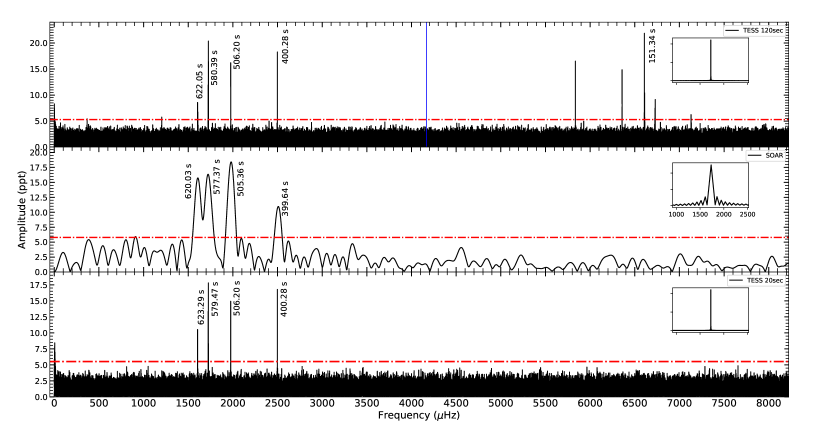
Figure 3: Fourier transform for TIC 304024058 for three different data sets. The result based on the 2-min (120-s) cadence TESS data is depicted in the top panel, while the bottom panel shows the FT for the 20-s cadence TESS data. The FT based on the SOAR telescope data (10 s integration time) is shown in the middle panel. The amplitude at FAP=1/1000 detection limit in each case is indicated by the horizontal dashed line, and the spectral window for each case is depicted as an inset plot. The blue vertical line in the top panel indicates the value of the Nyquist frequency.

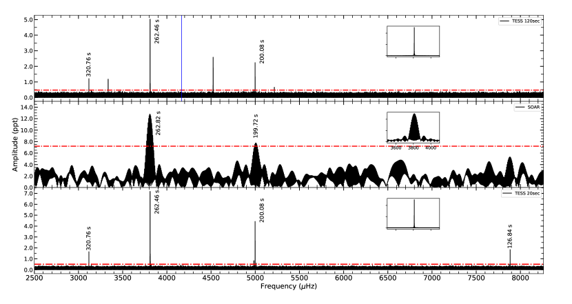
Figure 4: Fourier transforms for TIC 55650407 (same as Fig. 3).

As an example, in Figure 3 we show the FT for TIC 304024058 for 120 s cadence TESS data (top panel), ground-based observation from SOAR telescope with $\sim$15 s-cadence (middle panel) and 20 s cadence TESS data (bootm panel). The red horizontal line indicates the detection limit and the inset in each plot depicts the spectral window. For the 120 s cadence data in the top panel, the blue vertical line corresponds to the Nyquist frequency. Note that in this case, there are four significant peaks in the super-Nyquist region, with the peak at a period of 151.34 s being the one with the highest amplitude. However, these peaks are not seen in the ground-based observations, where only the peaks corresponding to periods between 400 s and 620 s are present. The same result is obtained when we include the 20 s cadence data from TESS. Thus, in this case, the sub-Nyquist aliases are confirmed to correspond to the intrinsic pulsation frequencies by ground-based observations and shorter-cadence TESS data.

A different result is found for TIC 55650407, as shown in Figure 4. The FT corresponding to the 120 s cadence TESS data shows two peaks with super-Nyquist frequencies, in particular one corresponding to a period of 200.08 s (see top panel). The same period is also present in the FT for the SOAR telescope data, shown in the middle panel of Figure 4, which confirms the existence of this period. On the other hand, the peak corresponding to the period of 320.76 s is not detected in the SOAR data, probably due to the much shorter SOAR observation run (3.72 h). Finally, the period with 200.08 s is also confirmed by the 20 s cadence TESS data, shown in the bottom panel of Figure 4. In addition, there is another peak at high frequencies with a corresponding period of 126.84 s that was not apparent in the 120-s data since the period is close to the exposure time.

4.2 TIC 20979953

TIC 20979953 was part of the target list for the TESS mission, but no 120 s or 20 s cadence data was taken for this object to date. We observed TIC 20979953 from the Pico do Dias observatory in two nights in 2020 (see Table 3) for a total of 6.76 h. The light curve and FT are presented in Figure 5 for the night of 2020-06-14 that spans for 3.4 h. From this dataset we detected three short periods of 259.68 s, 285.30 s and 365.64 s, compatible with a blue edge ZZ Ceti (Mukadam et al., 2006).

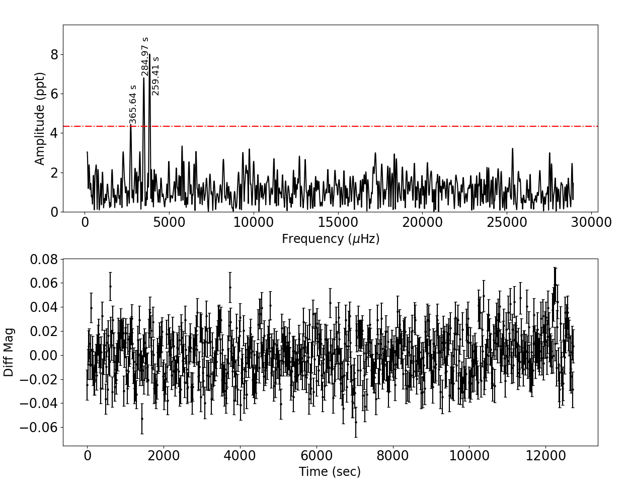
Figure 5: FT and light curve, top and bottom panel respectively, for TIC 20976653 based on data obtained from the Pico dos Dias observatory on 2020-06-14. The data spans for 3.4 h, with an integration time of 17 s.

5 Asteroseismological analysis

In this section we present an asteroseismological analysis of all objects presented in Tables 5 and 7. We employed an updated grid of DA white dwarf models, obtained from full evolutionary computations of the progenitor star. They were generated using the LPCODE evolutionary code (see Althaus et al., 2010b; Renedo et al., 2010; Romero et al., 2015, for details), that computes the evolution of the star from the zero-age main sequence, considering hydrogen and helium central burning and the giant phases. The grid corresponds to C/O-core white dwarf models with stellar masses between 0.493 M_⊙ to 1.05 M_⊙, with a hydrogen layer mass in the range of $\sim 4\times 10^{-4}$ to $\sim 10^{-10}$ M_∗, depending on the stellar mass. This model grid is an extended version of the model grid presented in Romero et al. (2019b) that includes new cooling sequences with stellar masses between 0.5 and 1.0 M_⊙, along with approximately eight hydrogen layer values for each sequence, depending on the stellar mass. For hydrogen envelopes thinner than $10^{-10}$M_∗ the outer convective zone will mix the hydrogen into the more massive helium layer before reaching the ZZ Ceti instabily strip, turning the star into a DB white dwarf (Ourique et al., 2020; Cunningham et al., 2020). For each model in our grid we computed non-radial g-mode pulsations, considering the adiabatic approximation, using the adiabatic version of the LP-PUL pulsation code (see Córsico & Althaus, 2006, for details).

For each object we search for an asteroseismological representative model that best matches the observed periods. To this end, we seek for the theoretical model that minimizes the quality function given by (Castanheira & Kepler, 2008),

$$S(M_{*},M_{\rm H},T_{\rm eff})=\sqrt{\sum_{i=1}^{N}{\rm min}\left[\frac{[\Pi_{i}^{\rm th}-\Pi_{i}^{\rm obs}]^{2}A_{i}}{\sum^{N}_{i=1}A_{i}}\right]},$$ (1)

where $N$ is the number of observed periods, $\Pi^{\rm th}_{i}$ is the theoretical period that better fits the observed period $\Pi^{\rm obs}_{i}$, and the amplitudes $A_{i}$ are used as weights for each period. In this way, the period fit is more influenced by those modes with larger observed amplitudes. We also compute other quality functions without the amplitude weighting, obtaining similar results.

For the eight objects with both TESS and ground-based data, we combine (add) the list of periods to perform the asteroseismological fit. We do not consider periods corresponding to harmonics or linear combinations, nor those modes that show super-Nyquist frequencies that were not confirmed by short-cadence observations. In the case where a period is detected both from TESS and ground-based observations, we consider the period value and amplitude corresponding to the TESS data. For the stars with spectroscopic mass below the minimum value of our C/O-core grid (0.493 M_⊙) we also perform an initial asteroseismological fit with He-core white dwarf models with stellar masses from 0.17 to 0.45 M_⊙ (Córsico et al., 2012), considering only canonical hydrogen envelopes and $\ell=1$ modes. Finally, if necessary, we consider the values of effective temperature and mass from Table 1 as an additional constrain in the fitting procedure. These last constrains are particularly important for objects with only one or two detected periods, which is the case for a substantial fraction of our objects. However, note that some particular short ($\lesssim$ 200 sec) periods can be strong constraints on their own, since they propagate in the inner parts of the star and are particularly sensitive to the inner structure.

The results of our asteroseimological fits are presented in Table 8. For each object we list the stellar mass, thickness of the hydrogen envelope and effective temperature for the seismological model, in columns 2, 3, and 4, respectively. Column 5 shows the values for the theoretical periods along with the corresponding harmonic degree $\ell$, and radial order $k$. Finally, the value of the quality function $S$ is listed in column 9. The first model listed is the one we choose to be the best-fitting model for that particular object.

Table 8: Best fit model for the new ZZ Cetis using the list of observed modes. The stellar mass, hydrogen envelope and effective temperature are listed in columns 2, 3 and 4, respectively. We list the theoretical periods in column 5, along with the harmonic degree and the radial order. The value of the quality function $S$ in seconds is listed in column 6.

TIC	M/M⊙	$-\log($MH/M${}_{*})$	Teff [K]	$\Pi$[s] ($\ell,k$)	$S$ [s]
5624184	0.493	4.85	11190	503.71 (1,7), 446.70 (2,12), 431.35 (1,16)	0.46
7675859	0.660	8.82	11710	356.26 (1,4), 798.51 (1,12), 742.93 (1,13)	0.28
$\cdots$	0.800	5.67	11660	356.33 (1,6), 799.19 (1,18), 743.00 (2,30)	0.37
8445665	0.675	4.35	10970	811.70 (1,17), 639.25 (1,13), 358.27 (2,12), 575.46 (2,21), 1019.48 (2,39)	1.51
13566624	0.705	6.15	12770	421.87 (1,4)	$\cdots$
21187072	0.660	5.55	11680	1074.2711 (1,21)	$\cdots$
24603397	0.542	6.83	12500	262.65 (1,2)	$\cdots$
29862344	0.609	8.33	11370	737.29 (1,12), 857.39 (1,14), 89890 (2,27)	0.12
33717565	0.609	5.74	12530	262.72 (1,3), 198.70 (1,2), 322.30 (2,9)	0.99
46847635	0.686	4.87	11930	415.82 (1,7)	$\cdots$
63281499	0.542	4.25	11610	320.37 (1,4), 384.76 (1,6)	0.60
65144290	0.632	4.46	11480	278.17 (1,4)	$\cdots$
72637474	0.542	4.94	11720	812.13 (1,14), 901.66 (1,16), 966.44 (1,17)	1.36
79353860	0.686	5.25	11390	945.54 (1,18), 842.57 (1,16), 525.10 (1,9)	0.35
116373308	0.609	8.33	11590	361.81 (1,4)	$\cdots$
$\cdots$	0.609	5.54	12160	361.78 (1,5)	$\cdots$
141976247	0.686	8.82	12910	261.71 (1,3)	$\cdots$
149863849	0.660	4.41	11380	397.99 (2,13), 419.15 (2,14), 569.41 (2,20), 487.83 (2,17)	0.55
156064657	0.493	6.84	10860	1418.07 (1,22), 1546.64 (1,24)	0.05
$\cdots$	0.358	3.26	9640	1418.71 (1,20), 1547.54 (1,22)	1.04
158068117	0.493	8.82	12150	268.453 (1,2)	$\cdots$
$\cdots$	0.303	2.90	9350	268.436 (1,2)	$\cdots$
167486543	0.820	4.93	12700	267.27 (1,5), 535.10 (1,13)	0.13
$\cdots$	0.745	5.37	12230	267.06 (1,4), 535.29 (1,11)	0.17
188087204	0.493	4.16	10640	743.05 (1,12), 657.69 (1,8), 544.00 (1,8), 500.07 (2,14)	1.19
207206751	0.570	4.28	10950	894.12 (2,30), 775.00 (2,26), 859.69 (1,16), 626.64 (1,11), 905.59 (1,17)	2.55
				1115.36 (2,38), 1277.72 (1,25), 864.29 (2,29), 809.88 (1,15)
220555122	0.686	6.34	11690	243.908 (1,3), 539.408 (1,9)	0.03
229581336	0.493	4.45	11310	1106.45 (2,34), 519.59 (2,15), 420.19 (1,6)	0.31
$\cdots$	0.400	3.18	10460	1106.60 (1,17), 514.61 (1,7), 421.31 (1,5)	1.75
230029140	0.593	5.04	11190	287.01 (1,3), 313.76 (1,4), 784.77 (1,14), 400.97 (1,6), 360.26 (2,10)	2.26
230384389	0.525	9.25	11410	(457.61 (1,5), (708.73 (1,10), 495.23 (2,12), 751.67 (2,20),	1.24
				1283.10 (1,20), 1632.01 (2,46)
231277791	0.570	5.45	11300	721.23 (1,13), 713.02 (2,23), 498.55 (1,8), 762.44 (2,25)	0.86
232979174	0.660	5.35	12020	282.66 (1,4)	$\cdots$
$\cdots$	0.493	3.72	11710	282.67 (1,3)	$\cdots$
238815671	0.690	5.26	11630	257.792 (1,3), 286.891 (1,4)	0.30
261400271	0.820	5.78	12390	295.25 (1,5), 382.68 (1,7)	0.36
287926830	0.570	4.28	11320	316.23 (1,4)	$\cdots$
313109945	0.675	9.25	9890	300.19 (1,3), 266.11 (1,2), 450.54 (2,11), 685.84 (2,19), 583.53 (2,16),	1.74
				410.63 (2,10), 250.03 (2,5)
317153172	0.621	6.34	11900	786.67 (2,25), 791.88 ( 1,14), 512.27 (1,8)	0.15
317620456	0.632	4.46	11010	260.86 (1,3), 429.24 (1,7)	0.19
343296348	0.548	4.27	11310	287.766 (1,3)	$\cdots$
344130696	0.632	9.34	11180	1018.70 (1,17), 1057.84 (1,18)	0.31
345202693	0.705	4.88	10670	587.86 (1,11), 789.31 (1,16), 833.79 (1,17), 833.79 (1,17)	0.51
353729306	0.690	6.94	11680	545.96 (1,9), 470.63 (1,7), 404.13 (2,12), 875.57 (2,30)	0.38
380298520	0.745	9.24	11550	549.86 (1,9)	$\cdots$
394015496	0.593	6.11	11570	309.79 (1,3)	$\cdots$
415337224	0.609	4.85	10100	936.88 (2, 32), 550.73 (1,9), 953.11 (1,18)	0.37
428670887	0.609	5.24	11500	298.14 (1,4)	$\cdots$
441500792	0.705	4.48	11260	617.31 (1,13), 786.32 (1,17), 980.86 (1,22)	0.53
$\cdots$	0.745	9.28	11460	618.21 (2,20), 786.52 (2,26), 981.21 (2,33)	0.41
442962289	0.837	5.00	12120	418.75 (1,9), 652.00 (1,16), 498.87 (2,22)	1.02
610337553	0.609	6.33	10970	759.49 (1,13), 922.81 (1,16)	0.12
631161222	0.609	5.44	11400	368.60 (1,5), 403.39 (1,6), 467.10 (1,7), .79,27 (1,12), 708.31 (1,13)	0.60
631344957	0.550	4.84	11550	363.144 (1,5)	$\cdots$
632543979	0.660	5.15	11250	461.54 (2,15), 783.90 (1,15), 736.26 (2,25), 652.00 (2,22), 797,03 (1,14)	0.50
651462582	0.593	5.79	10780	817.49 (1,14), 683.29 (1,11), 1019.36 (1,18)	0.74
661119673	0.570	4.55	11600	626.42 (1,11)	$\cdots$
685410570	0.609	4.95	10900	965.62 (1,18), 812.60 (1,15), 557.09 (1,9)	0.30
686044219	0.639	4.12	11130	913.75 (1,19), 735.99 (1,15), 875.08 (1,18)	0.58

Table 9: continued

TIC	M/M⊙	MH/M∗	Teff [K]	$\Pi$[s] ($\ell,k$)	$S$ [s]
712406809	0.646	4.12	10820	827.83 (1,17), 510.53 (2,18), 872.93 (1,18), 118.57 (1,1), 623.51 (1,12)	1.15
724128806	0.542	6.36	10910	290.18 (1,3)	$\cdots$
$\cdots$	0.251	2.92	10410	290.19 (1,2)	$\cdots$
733030384	0.660	6.24	12390	275.48 (1,4), 411.63 (1,6)	0.24
800153845	0.593	7.34	11780	877.99 (1,14), 712.38 (1,11)	0.29
804835539	0.609	4.45	10990	1007.21 (1,20)	$\cdots$
804899734	0.609	5.35	11780	394.82 (1,6)	$\cdots$
951016050	0.660	4.86	10850	818.58 (1,12), 644.56 (1,16)	0.11
1001545355	0.542	6.13	11380	516.47 (1,14), 763.42 (1,22), 955.84 (1,28), 1055.98 (1,31)	1.52
1102242692	0.609	5.44	11200	1009.13 (1,19), 406.18 (1,6)	0.07
1102346472	0.548	4.27	10970	458.13 (1,7)	$\cdots$
1108505075	0.579	5.34	11310	693.40 (1,12), 1323.63 (1,25), 1801.95 (1,35)	0.14
1173423962	0.690	7.14	10940	618.45 (1,10), 794.75 (1,14)	0.08
1201194272	0.609	4.11	11470	840.92 (1,17)	$\cdots$
1309155088	0.609	4.19	10710	769.05 (1,15)	$\cdots$
1989258883	0.609	6.04	11110	909.03 (1,16)	$\cdots$
2026445610	0.525	3.79	11240	825.42 (1,15), 317.77 (1,4)	0.09

Table 10: Best fit model for the new ZZ Cetis using the list of modes from TESS and/or ground based observations. The stellar mass, hydrogen envelope and effective temperature are listed in columns 2, 3 and 4, respectively. We list the theoretical periods in column 5, along with the harmonic degree and the radial order. The value of the quality function $S$ in seconds is listed in column 6. *No variability detected with TESS down to FAP=1/1000.

TIC	M/M⊙	$-\log($MH/M${}_{*})$	Teff [K]	$\Pi$[s] ($\ell,k$)	$S$ [s]
20979953	0.632	8.33	11130	259.77 (1,2), 285.27 (1,3), 365.57 (1,4)	0.07
	0.593	3.93	12200	258.59 (1,3), 285.59 (1,4), 365.79 (1,6)	0.73
55650407	0.570	3.82	12600	316.93 (1,5), 262.34 (1,3), 203.39 (2,5), 125.17 (1,1)	2.28
	0.542	5.63	12980	320.95 (1,4), 263.45 (1,3), 201.75 (2,4), 125.17 (2,2)	1.25
273206673	0.686	4.60	11170	582.89 (1,11), 825.86 (1,17), 693.35 (1,14), 744.84 (2,27),	2.32
				894.33 (2,33), 464.05 (1,8), 841.82 (2,31), 508.83 (2,18),
				688.38 (2,25),665,46 (2,24), 873.64 (1,18), 1033.89 (2,38)
282783760	0.593	3.93	12270	258.14 (1,3), 284.80 (1,4), 307.69 (1,4)	1.06
	0.493	4.35	11710	257.84 (2,6), 283.94 (1,3), 308.38 (2,8)	0.45
304024058	0.542	4.15	12020	623.34 (2,20), 579.09 (1,10), 504.59 (2,16), 400.22 (2,12)	0.80*
	0.593	6.33	11400	623.53 (2,19), 578.50 (1,9), 506.82 (2,15), 401.33 (2,11)	0.83*
370239521	0.770	8.66	11010	822.34 (1,15), 806.91 (2,27), 576.79 (1,10), 565.95 (2,18), 274.34 (2,7),	2.05
				895.47 (1,17), 732.69 (2,24), 779.20 (2,26), 932.76 (1,18)
	0.721	5.08	11240	821.03 (2,31), 808.78 (1,17), 578.19 (2,21), 569.39 (1,11), 276.93 (1,4),	2.57
				896.39 (1,19), 729.89 (1,15), 772.40 (2,29), 932.48 (1,20)
1989866634	0.820	7.36	10960	613.81 (1,12), 568.43 (1,11), 364.26 (2,12), 899.66 (2,33),	1.47
				227.90 (1,3), 500.76 (1,9), 973.80 (2,36)
	0.609	4.75	11250	614.31 (1,11), 572.38 (2,19), 359.98 (2,11), 895.59 (2,31),	2.03
				227.89 (2,6), 495.11 (1,8), 975.76 (1,19)
2055504010	0.705	5.75	11030	990.45 (1,20), 818.45 (1,16), 774.90 (2,27)	0.21

5.1 Rotation Periods

White dwarf stars are considered slow rotators, with rotation periods between a few hours and several days (see for instance Kepler & Romero, 2017). By considering the frequency separation we can estimate the rotation period of the white dwarf star, following the equation (Cowling & Newing, 1949; Ledoux, 1951):

$$\frac{1}{P_{\rm rot}}=\frac{\Delta\nu_{k,\ell,m}}{m(1-C_{k\ell})}$$ (2)

where $m$ is the azimuthal number and $C_{k\ell}$ is the rotational splitting coefficient given by:

$$C_{k,\ell}=\frac{\int_{0}^{R_{*}}\rho r^{2}[2\xi_{r}\xi_{t}+\xi_{t}^{2}dr}{\int_{0}^{R_{*}}\rho r^{2}[\xi_{r}^{2}+\ell(\ell+1)\xi_{t}^{2}]dr}$$ (3)

where $\rho$ is the density, $r$ is the radius and $\xi_{r}$ and $\xi_{t}$ are the radial and horizontal displacement of the material.

Since all our datasets have very high duty cycles, our TESS data is generally free of aliasing and can readily reveal patterns of even frequency spacing in the Fourier transform that can reveal the stellar rotation rate (e.g. Kawaler, 2004)). Identifying rotationally split multiplets is also an excellent way to identify the spherical degree and azimuthal order of the modes present (e.g., Winget et al. 1991, 1994).

We detect rotationally split multiplets in four new ZZ Cetis with TESS data. The list of objects with detected $\ell=1$ multiplets is presented in Table 11. We list the frequencies corresponding to the multiplet, the $C_{k\ell}$ (determined from our best-fit asteroseismic solution in Section 5), and the resultant mean stellar rotation period. In Figure 6 we show all four stars with rotationally split multiplets; these are the only multiplets we identify in each star.

Table 11: List of objects with detected rotational splittings, also shown in Figure 6. For each object we list the frequency that form the multiplet (col 2), the value of the $C_{k\ell}$ obtained from the asteroseismologial representative model (col 3) and the mean rotation period (col 4).

TIC	$\nu$ [$\mu$Hz]	$C_{k\ell}$	$\bar{P}_{\rm rot}$
7675859	2830.86, 2808.28, 2775.31	0.487	5.20 h
21187072	933.93, 930.86, 928.63	0.495	2.24 d
343296348	3481.29, 3475.12, 3468.97	0.458	1.02 d
394015496	3233.00, 3227.99, 3223.00	0.463	1.24 d

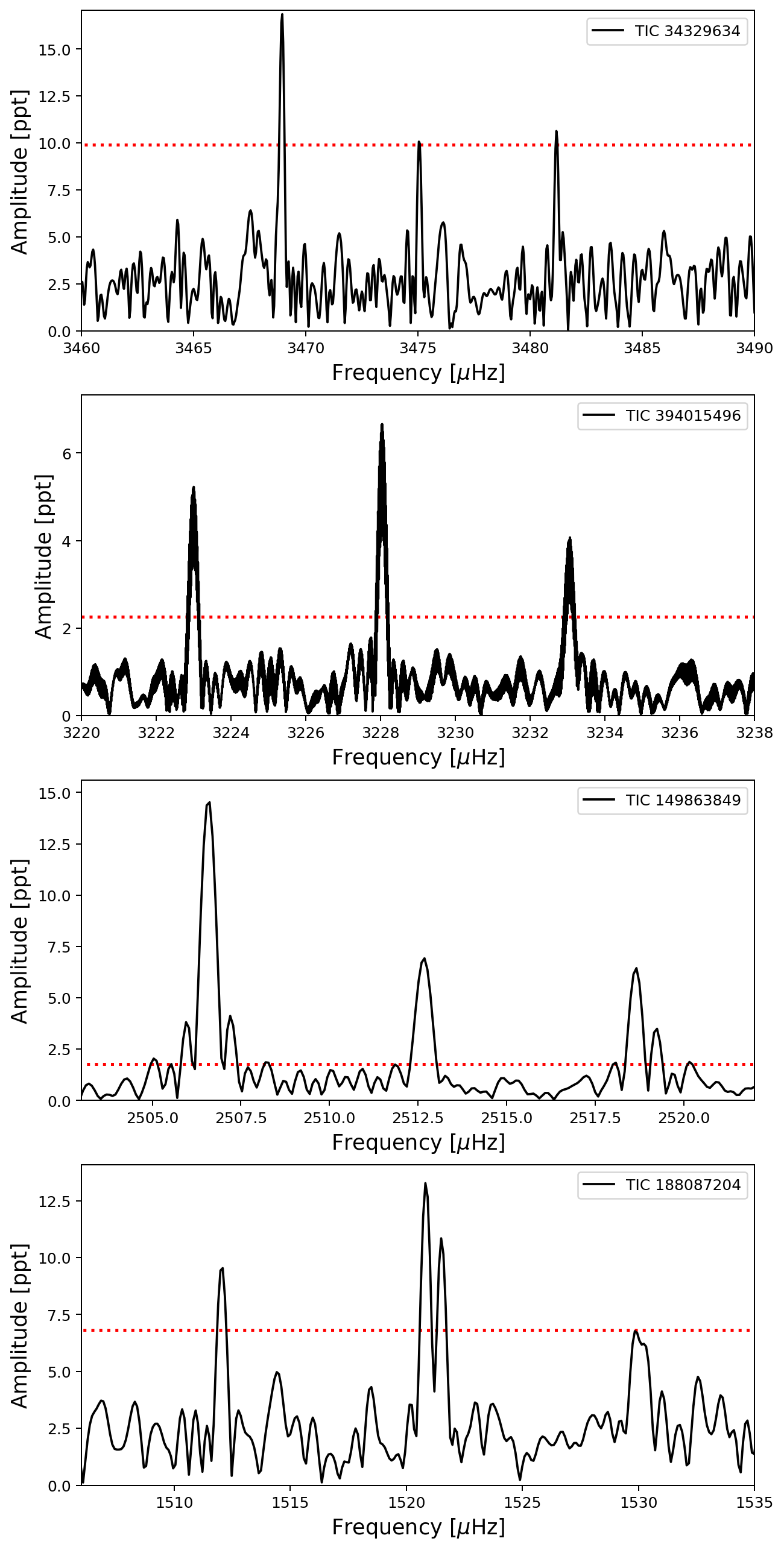
Figure 6: FT showing the three peaks corresponding to the triplet for four objects listed in Table 11.

The lack of aliasing from space-based data from Kepler and TESS has enabled the detection of rotational splittings for a much larger sample of pulsating white dwarfs. Among the first 27 ZZ Cetis observed by Kepler and K2, patterns from rotational splitting was observed in 20 ZZ Cetis (74 per cent, Hermes et al. 2017a). Unfortunately, we only detect patterns from rotation in just 4 of 74 ZZ Cetis ($<$6 per cent) in this manuscript.

This decrease in detection among ZZ Cetis with TESS can be understood in two ways. First, we are generally limited to a Nyquist frequency of 4166.67 $\mu$Hz (1/240 s^-1) with our 2-min-cadence data, so we are biased against the shortest-period ZZ Cetis that more commonly exhibit clear rotational splittings (Hermes et al., 2017b). Additionally, and likely most significantly, the noise limits (and thus the lowest amplitudes we can significantly detect) from TESS data on our ZZ Cetis are generally an order of magnitude worse than the 27 ZZ Cetis in Hermes et al. (2017a) — in that work the mean significant threshold is 0.75 ppt, whereas the mean value in this work is 8.4 ppt. We generally have the frequency resolution to detect 0.5-2.0-day rotation periods, but are only able to detect the highest-amplitude modes, and thus miss identifying many rotationally split multiples.

With additional coverage and high-enough cadence to detect shorter-period pulsations, we are optimistic that future observations of white dwarfs with the 20-second cadence will enable us to detect rotationally split modes in far more ZZ Cetis going forward.

6 Analysis of the sample

In this section we analyse the main results of our sample of 75 new bright ZZ Ceti stars reported in this paper, corresponding to the 74 objects observed by TESS and TIC 20976653. In Figure 7 we compare the values for the effective temperature from photometry + parallax from Gaia (x-axis) and asteroseismology (y-axis). We consider that the internal uncertainties from the asteroseismological fitting procedure are 100 K, 200 K, and 300 K, for effective temperatures, below $11\,400$ K, between $11\,400$ and $11\,800$ K, and higher than $11\,800$ K, respectively. The uncertainties for the photometric effective temperature are taken from Table 1. We depict the objects with one or two detected periods with blue squares, while the objects with more than two detected periods are depicted with black circles. As can be seen from this figure, the data clusters around the 1:1 correspondence line. The outliers correspond to those objects with photometric mass below 0.45 M_⊙ and those with photometric effective temperature higher than $14\,000$ K. The Pearson coefficient is $r$ = 0.1154, which indicates a negligible correlation. We do not expect a full correlation since both determinations come from different data sets: the three photometric filters and parallax for the photometric determination, and the detected period spectrum for the seismological determination.

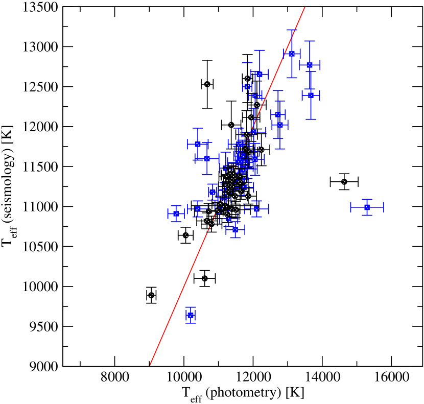
Figure 7: Comparison between the effective temperature obtained from Gaia photometry + parallax (see Table 1) and the asteroseismological fit (see Table 8). The red line indicates the 1:1 correspondence. Blue squares correspond to objects with one or two detected periods, and black circle to those with more than two detected periods.

Figure 8 shows the comparison between the stellar mass from photometry + parallax (x-axis) from Gaia and the value obtained from our seismological fit. The black circles correspond to the 36 objects with more than two detected periods, while the blue squares depict the 37 objects with one or two detected periods; these blue squares have seismological results that are less reliable since there are so few constraints from pulsation periods. Note that we do not include TIC 345202693 since this object has no reliable photometric parameters due to its main sequence companion. The uncertainties for the seismological mass correspond to internal uncertainties from the fitting procedure. Although the points are around the 1:1 correspondence line, there is a large scatter. The Pearson coefficient is $r$= 0.6020, corresponding to a moderate correlation.

The larger discrepancies between the photometric and seismological masses appear for the objects with photometric mass below 0.45 M_⊙. Since our model grid do not consider white dwarf models with stellar masses below 0.493 M_⊙, we do not expect an agreement between the two determinations.

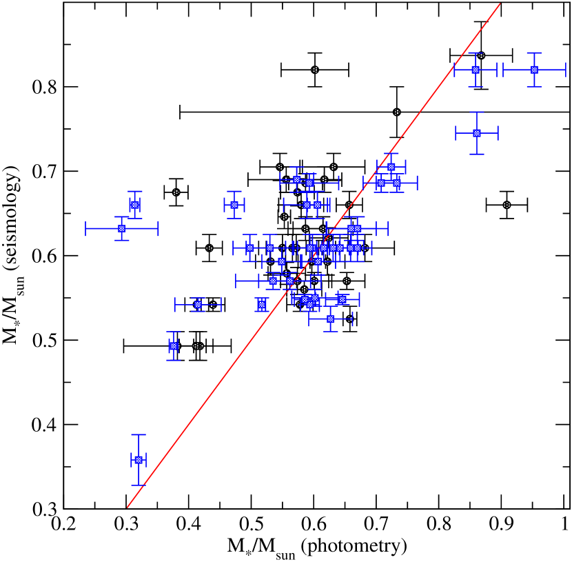
Figure 8: Comparison between the stellar mass obtained from Gaia photometry + parallax (see Table 1) and the asteroseismological fit (see Table 8). The red line indicates the 1:1 correspondence. The objects with one or two detected periods are depicted as blue squares, while those with more than two detected periods are depicted with black circles.

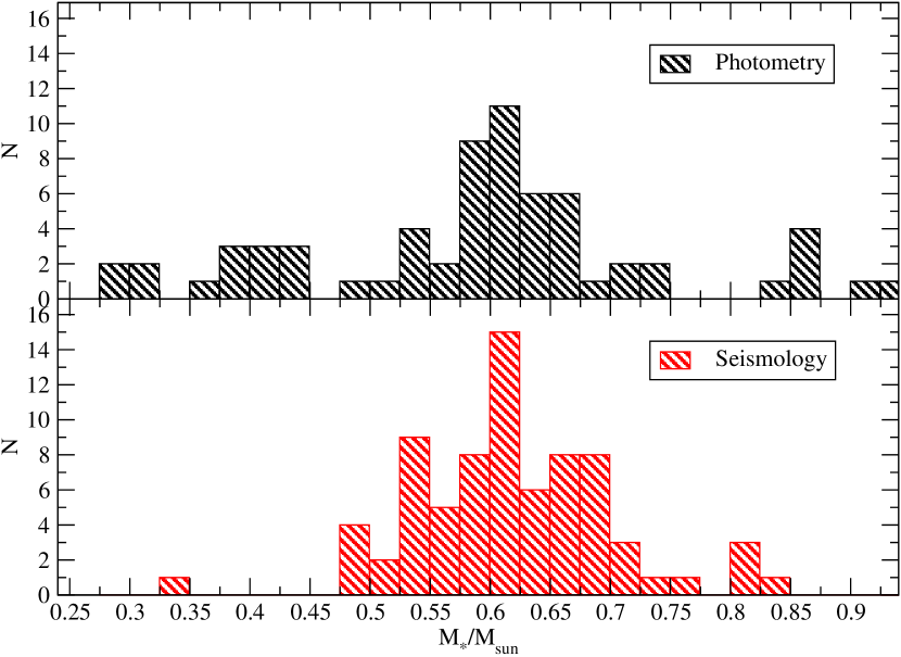
Figure 9: Histograms showing the distribution of the photometric (top) and seismological (bottom) stellar mass.

The mass distribution for our 74 objects is shown in Figure 9, where we show the histograms for the photometric (top panel) and the seismological (low panel) stellar mass. As expected, the mass distribution from photometry extends further to lower stellar masses, than the one from asteroseismology. In both cases, most of the object show stellar masses between 0.5 and 0.7 M_⊙.

The mean photometric mass is $\langle M_{\rm phot}\rangle=$ 0.588$\pm$ 0.038 M_⊙, while for the seismological mass, the value is $\langle M_{\rm seis}\rangle=$ 0.621$\pm$0.015 M_⊙. Even though both values agree within the uncertainties, the seismological mean mass is $\sim$ 5 per cent higher than the photometric value. If we consider only the 61 objects with photometric masses larger than 0.49 M_⊙, the values are $\langle M_{\rm phot}\rangle=$ 0.631$\pm$ 0.040 M_⊙, and $\langle M_{\rm seis}\rangle=$ 0.635$\pm$0.015 M_⊙, with an agreement within 1$\sigma$. Finally, these values for the photometric and seismological mean mass are in agreement with the mean mass of 351 known ZZ Ceti stars shown in Figure 1 with coloured symbols, being $\langle M_{*}\rangle=$ 0.644$\pm$0.034 M_⊙.

7 Conclusions

In this work we present the discovery of 74 new ZZ Ceti stars, based on the data from the TESS mission, from Sector 1 to Sector 39. In addition, we perform follow-up observations for 11 objects from ground-based facilities, i.e., the Konkoly observatory (1.0-m), SOAR telescope (4.1-m), Perkins telescope (1.8-m) and the Pico dos Dias observatory (1.6-m), which in most cases, increased the number of detected periods. The new ZZ Cetis are much brighter than the average previously known ZZ Ceti, and in this sample range from $13.5<G<17.5$ mag. In addition, we detected one additional new ZZ Ceti, TIC 20979953, from ground-based observations showing three pulsation periods. This object has no observations yet with TESS.

We perform a preliminary asteroseismological study of the new sample, and determine their seismological stellar mass, effective temperature and hydrogen envelope mass, among other structural parameters, depending on the number of detected periods. Extensive observations are required to detect a significant number of periods for a more meaningful seismological study, which will in many cases be enabled simply by adding future TESS data, which will improve noise limits to allow us to detect more modes.

We detected rotational splittings from TESS data for four objects, TIC 7675859, TIC 21187072, TIC 343296348 and TIC 394015496. Our derived rotation periods ($0.2-2.2$ days) are roughly compatible with previous estimates of other white dwarf stars.

The mean stellar mass of our sample from photometry and seismology are $\langle M_{\rm phot}\rangle=$ 0.588$\pm$ 0.038 M_⊙ and $\langle M_{\rm seis}\rangle=$ 0.621$\pm$0.015 M_⊙, respectively. Considering the 61 objects with photometric masses above 0.49 M_⊙, the values are $\langle M_{\rm phot}\rangle=$ 0.631$\pm$ 0.040 M_⊙, and $\langle M_{\rm seis}\rangle=$ 0.635$\pm$0.015 M_⊙, respectively. Both values are in agreement with the mean spectroscopic mass of a sample of 351 known ZZ Ceti depicted in Figure 1, $\langle M_{*}\rangle=$ 0.644$\pm$0.034 M_⊙.

These 75 new bright ZZ Cetis increase the sample of known pulsating DA white dwarf stars by roughly 20 per cent, and our understanding of their interiors will only improve with additional observations from the TESS mission.

Data Availability

Data from TESS is available at the MAST archive https://mast.stsci.edu/search/hst/ui/$#$/. Ground based data will be shared on reasonable request to the corresponding author.

References

- Althaus et al. (2010a) Althaus L. G., Córsico A. H., Isern J., García-Berro E., 2010a, A&ARv, 18, 471
- Althaus et al. (2010b) Althaus L. G., Córsico A. H., Bischoff-Kim A., Romero A. D., Renedo I., García-Berro E., Miller Bertolami M. M., 2010b, ApJ, 717, 897
- Bell et al. (2017) Bell K. J., Hermes J. J., Vanderbosch Z., Montgomery M. H., Winget D. E., Dennihy E., Fuchs J. T., Tremblay P. E., 2017, ApJ, 851, 24
- Bell et al. (2019) Bell K. J., et al., 2019, A&A, 632, A42
- Bergeron et al. (1995) Bergeron P., Saumon D., Wesemael F., 1995, ApJ, 443, 764
- Bergeron et al. (1997) Bergeron P., Ruiz M. T., Leggett S. K., 1997, ApJS, 108, 339
- Bergeron et al. (2019) Bergeron P., Dufour P., Fontaine G., Coutu S., Blouin S., Genest-Beaulieu C., Bédard A., Rolland B., 2019, ApJ, 876, 67
- Bida et al. (2014) Bida T. A., Dunham E. W., Massey P., Roe H. G., 2014, in Ramsay S. K., McLean I. S., Takami H., eds, Society of Photo-Optical Instrumentation Engineers (SPIE) Conference Series Vol. 9147, Ground-based and Airborne Instrumentation for Astronomy V. p. 91472N, doi:10.1117/12.2056872
- Bognar & Sodor (2016) Bognar Z., Sodor A., 2016, Information Bulletin on Variable Stars, 6184, 1
- Bognár et al. (2020) Bognár Z., et al., 2020, A&A, 638, A82
- Brickhill (1991) Brickhill A. J., 1991, MNRAS, 251, 673
- Castanheira & Kepler (2008) Castanheira B. G., Kepler S. O., 2008, MNRAS, 385, 430
- Chambers et al. (2016) Chambers K. C., et al., 2016, arXiv e-prints, p. arXiv:1612.05560
- Clemens (1993) Clemens J. C., 1993, Baltic Astronomy, 2, 407
- Clemens et al. (2004) Clemens J. C., Crain J. A., Anderson R., 2004, in Moorwood A. F. M., Iye M., eds, Society of Photo-Optical Instrumentation Engineers (SPIE) Conference Series Vol. 5492, Ground-based Instrumentation for Astronomy. pp 331–340, doi:10.1117/12.550069
- Córsico & Althaus (2006) Córsico A. H., Althaus L. G., 2006, A&A, 454, 863
- Córsico et al. (2012) Córsico A. H., Romero A. D., Althaus L. G., Hermes J. J., 2012, A&A, 547, A96
- Córsico et al. (2019) Córsico A. H., Althaus L. G., Miller Bertolami M. M., Kepler S. O., 2019, A&ARv, 27, 7
- Córsico et al. (2021) Córsico A. H., et al., 2021, A&A, 645, A117
- Cowling & Newing (1949) Cowling T. G., Newing R. A., 1949, ApJ, 109, 149
- Cunningham et al. (2020) Cunningham T., Tremblay P.-E., Gentile Fusillo N. P., Hollands M., Cukanovaite E., 2020, MNRAS, 492, 3540
- Currie et al. (2014) Currie M. J., Berry D. S., Jenness T., Gibb A. G., Bell G. S., Draper P. W., 2014, in Manset N., Forshay P., eds, Astronomical Society of the Pacific Conference Series Vol. 485, Astronomical Data Analysis Software and Systems XXIII. p. 391
- Dolez & Vauclair (1981) Dolez N., Vauclair G., 1981, A&A, 102, 375
- Eastman et al. (2010) Eastman J., Siverd R., Gaudi B. S., 2010, PASP, 122, 935
- Eisenstein et al. (2006) Eisenstein D. J., et al., 2006, ApJS, 167, 40
- Fontaine & Brassard (2008) Fontaine G., Brassard P., 2008, PASP, 120, 1043
- Fontaine et al. (2001) Fontaine G., Brassard P., Bergeron P., 2001, PASP, 113, 409
- Gaia Collaboration et al. (2018) Gaia Collaboration et al., 2018, A&A, 616, A10
- Gentile Fusillo et al. (2019) Gentile Fusillo N. P., et al., 2019, MNRAS, 482, 4570
- Gentile Fusillo et al. (2021) Gentile Fusillo N. P., et al., 2021, MNRAS, 508, 3877
- Gianninas et al. (2011) Gianninas A., Bergeron P., Ruiz M. T., 2011, ApJ, 743, 138
- Goldreich & Wu (1999) Goldreich P., Wu Y., 1999, ApJ, 511, 904
- Guidry et al. (2021) Guidry J. A., et al., 2021, ApJ, 912, 125
- Hermes et al. (2017a) Hermes J. J., et al., 2017a, ApJS, 232, 23
- Hermes et al. (2017b) Hermes J. J., et al., 2017b, ApJ, 841, L2
- Horne (1986) Horne K., 1986, PASP, 98, 609
- Istrate et al. (2014) Istrate A. G., Tauris T. M., Langer N., 2014, A&A, 571, A45
- Istrate et al. (2016) Istrate A. G., Marchant P., Tauris T. M., Langer N., Stancliffe R. J., Grassitelli L., 2016, A&A, 595, A35
- Jenkins et al. (2016) Jenkins J. M., et al., 2016, in Chiozzi G., Guzman J. C., eds, Society of Photo-Optical Instrumentation Engineers (SPIE) Conference Series Vol. 9913, Software and Cyberinfrastructure for Astronomy IV. p. 99133E, doi:10.1117/12.2233418
- Kawaler (2004) Kawaler S. D., 2004, in Maeder A., Eenens P., eds, IAU Conference Series Vol. 215, Stellar Rotation. p. 561
- Kepler (1993) Kepler S. O., 1993, Baltic Astronomy, 2, 515
- Kepler & Romero (2017) Kepler S. O., Romero A. D., 2017, in European Physical Journal Web of Conferences. p. 01011 (arXiv:1706.07020), doi:10.1051/epjconf/201715201011
- Kepler et al. (2019) Kepler S. O., et al., 2019, MNRAS, 486, 2169
- Kilic et al. (2007) Kilic M., Stanek K. Z., Pinsonneault M. H., 2007, ApJ, 671, 761
- Kilic et al. (2020) Kilic M., Bergeron P., Kosakowski A., Brown W. R., Agüeros M. A., Blouin S., 2020, ApJ, 898, 84
- Kleinman et al. (2013) Kleinman S. J., et al., 2013, ApJS, 204, 5
- Koester (2009) Koester D., 2009, A&A, 498, 517
- Koester (2010) Koester D., 2010, Mem. Soc. Astron. Italiana, 81, 921
- Koester et al. (2009) Koester D., Voss B., Napiwotzki R., Christlieb N., Homeier D., Lisker T., Reimers D., Heber U., 2009, A&A, 505, 441
- Kowalski & Saumon (2006) Kowalski P. M., Saumon D., 2006, ApJ, 651, L137
- Ledoux (1951) Ledoux P., 1951, ApJ, 114, 373
- Lenz & Breger (2004) Lenz P., Breger M., 2004, in Zverko J., Ziznovsky J., Adelman S. J., Weiss W. W., eds, IAU Conference Series Vol. 224, The A-Star Puzzle. pp 786–790, doi:10.1017/S1743921305009750
- Liebert et al. (2005) Liebert J., Bergeron P., Holberg J. B., 2005, ApJS, 156, 47
- Limoges et al. (2013) Limoges M. M., Lépine S., Bergeron P., 2013, AJ, 145, 136
- Marsh (1989) Marsh T. R., 1989, PASP, 101, 1032
- Montgomery et al. (2020) Montgomery M. H., Hermes J. J., Winget D. E., Dunlap B. H., Bell K. J., 2020, ApJ, 890, 11
- Mukadam et al. (2006) Mukadam A. S., Montgomery M. H., Winget D. E., Kepler S. O., Clemens J. C., 2006, ApJ, 640, 956
- Murphy (2015) Murphy S. J., 2015, MNRAS, 453, 2569
- Ourique et al. (2020) Ourique G., Kepler S. O., Romero A. D., Klippel T. S., Koester D., 2020, MNRAS, 492, 5003
- Pelisoli & Vos (2019) Pelisoli I., Vos J., 2019, MNRAS, 488, 2892
- Pych (2004) Pych W., 2004, PASP, 116, 148
- Raddi et al. (2017) Raddi R., et al., 2017, MNRAS, 472, 4173
- Renedo et al. (2010) Renedo I., Althaus L. G., Miller Bertolami M. M., Romero A. D., Córsico A. H., Rohrmann R. D., García-Berro E., 2010, ApJ, 717, 183
- Ricker et al. (2014) Ricker G. R., et al., 2014, in Oschmann Jacobus M. J., Clampin M., Fazio G. G., MacEwen H. A., eds, Society of Photo-Optical Instrumentation Engineers (SPIE) Conference Series Vol. 9143, Space Telescopes and Instrumentation 2014: Optical, Infrared, and Millimeter Wave. p. 914320 (arXiv:1406.0151), doi:10.1117/12.2063489
- Romero et al. (2015) Romero A. D., Campos F., Kepler S. O., 2015, MNRAS, 450, 3708
- Romero et al. (2019a) Romero A. D., Kepler S. O., Joyce S. R. G., Lauffer G. R., Córsico A. H., 2019a, MNRAS, 484, 2711
- Romero et al. (2019b) Romero A. D., et al., 2019b, MNRAS, 490, 1803
- Romero et al. (2021) Romero A. D., Lauffer G. R., Istrate A. G., Parsons S. G., 2021, MNRAS,
- Science Software Branch at STScI (2012) Science Software Branch at STScI 2012, PyRAF: Python alternative for IRAF (ascl:1207.011)
- Su et al. (2017) Su J., Fu J., Lin G., Chen F., Khokhuntod P., Li C., 2017, ApJ, 847, 34
- Subasavage et al. (2008) Subasavage J. P., Henry T. J., Bergeron P., Dufour P., Hambly N. C., 2008, AJ, 136, 899
- Tremblay & Bergeron (2009) Tremblay P. E., Bergeron P., 2009, ApJ, 696, 1755
- Tremblay et al. (2010) Tremblay P. E., Bergeron P., Kalirai J. S., Gianninas A., 2010, ApJ, 712, 1345
- Tremblay et al. (2011) Tremblay P. E., Bergeron P., Gianninas A., 2011, ApJ, 730, 128
- Tremblay et al. (2013) Tremblay P. E., Ludwig H. G., Steffen M., Freytag B., 2013, A&A, 559, A104
- Uzundag et al. (2021) Uzundag M., et al., 2021, A&A, 655, A27
- Vincent et al. (2020) Vincent O., Bergeron P., Lafrenière D., 2020, AJ, 160, 252
- Wang et al. (2020) Wang K., Zhang X., Dai M., 2020, ApJ, 888, 49
- Winget & Kepler (2008) Winget D. E., Kepler S. O., 2008, ARA&A, 46, 157
- Winget et al. (1982) Winget D. E., van Horn H. M., Tassoul M., Fontaine G., Hansen C. J., Carroll B. W., 1982, ApJ, 252, L65
- Winget et al. (1991) Winget D. E., et al., 1991, ApJ, 378, 326
- Winget et al. (1994) Winget D. E., et al., 1994, ApJ, 430, 839