A Parameter-Free Differential Evolution Algorithm for the Analytic Continuation of Imaginary Time Correlation Functions

Abstract

We report on Differential Evolution for Analytic Continuation (DEAC): a parameter-free evolutionary algorithm to generate the dynamic structure factor from imaginary time correlation functions. Our approach to this long-standing problem in quantum many-body physics achieves enhanced spectral fidelity while using fewer compute (CPU) hours. The need for fine-tuning of algorithmic control parameters is eliminated by embedding them within the genome to be optimized for this evolutionary computation based algorithm. Benchmarks are presented for models where the dynamic structure factor is known exactly, and experimentally relevant results are included for quantum Monte Carlo simulations of bulk ⁴He below the superfluid transition temperature.

I Introduction

Imaginary time correlation functions can be extended to the real time domain via analytic continuation Pathria and Beale (2022). However, the process to achieve accurate spectral functions from quantum Monte Carlo (QMC) data is a notoriously ill-posed inverse problem as a result of the stochastic uncertainty that ensures the equivalent likelihood of many different possible reconstructions through direct inverse Laplace transformations.

Current approaches to the inverse problem are labeled by a zoo of acronyms and include: the average spectrum method (ASM) Ghanem and Koch (2020), stochastic optimization with consistent constraints (SOCC) Goulko et al. (2017), genetic inversion via falsification of theories (GIFT) Bertaina et al. (2017); Vitali et al. (2010), the famous maximum entropy method (MEM) Jarrell and Gubernatis (1996), and the fast and efficient stochastic optimization method (FESOM) Bao et al. (2016). The ASM approach performs a functional average over all admissible spectral functions, while SOCC uses random updates to the spectrum consistent with error bars on the input data. The GIFT method uses a genetic algorithm with many algorithmic control parameters. The traditionally used MEM utilizes Bayesian inference and is further described in Section III.1. Finally, a state-of-the-art approach FESOM adds random noise to proposed spectra at each iteration, averaging the spectra when a level of fitness is reached, and is further described in Section III.2. More recent work has focused on applying machine learning techniques Fournier et al. (2020); Raghavan et al. (2021); Kades et al. (2020) with limited success for particular types of imaginary time correlations.

In this paper we introduce a new method: the differential evolution for analytic continuation (DEAC) algorithm, to achieve reconstructed dynamic structure factors $S({\bf\it q},\omega)$ from the imaginary time intermediate scattering function. Similar to the GIFT method Bertaina et al. (2017), a population of candidate spectral functions is maintained whose average fitness is improved through recombination over several generations. Control parameters are adjusted using self adaptive techniques. This new method is validated against nine multi-peak spectra at finite temperature and compared with two other robust and commonly used methods, MEM and FESOM. Our algorithm performs well in terms of speed, accuracy, and ease of use. These three strengths unlock new avenues for scientific discovery through greater utilization of computational resources and better fidelity of the reconstructed spectra.

The remainder of this paper is organized as follows. We begin with a comprehensive description of the inverse problem, the construction of simulated quantum Monte Carlo data, and the method used to generate imaginary time intermediate scattering data for superfluid ⁴He. Details are then given for our implementation of the two competing approaches, before proceeding to a detailed discussion of our evolutionary algorithm. A careful comparison of the results and performance of the DEAC algorithm with both the maximum entropy and stochastic optimization methods is provided for simulated data sets containing ubiquitous spectral features. Moving beyond simulated data, results are shown for the bulk ⁴He spectrum below the superfluid transition temperature. We conclude with an analysis of the resulting spectral functions and discussion of the advantages of each method. Scripts and data used in analysis and plotting as well as details to download the source code for the three analytic continuation methods explored are available online Nichols (2021a).

II Model and Data

II.1 The Inverse Problem

The dynamic structure factor is a measure of particle correlations in space and time Pathria and Beale (2022). It is defined as the temporal Fourier transform:

$$S({\bf\it q},\omega)=\frac{1}{2\pi}\int_{-\infty}^{\infty}F({\bf\it q},t)\exp(i\omega t)\mathrm{d}t$$ (1)

for wave vector ${\bf\it q}$ and frequency $\omega$, where $F({\bf\it q},t)=\frac{1}{N}\langle\rho_{{\bf\it q}}(t)\rho_{\bar{{\bf\it q}}}(0)\rangle$ is the intermediate scattering function, which can be written more explicitly as

$$F({\bf\it q},t)=\frac{1}{N}\expectationvalue{\sum_{j,l}e^{-i{\bf\it q}\cdot{\bf\it r}_{j}(t)}e^{i{\bf\it q}\cdot{\bf\it r}_{l}(0)}}$$ (2)

in units with Planck’s constant $\hbar=1$ and the Boltzmann constant $k_{B}=1$ for time-dependent particle positions ${\bf\it r}(t)$.

A determination of the intermediate scattering function in imaginary time is found by using the detailed balance condition of the dynamic structure factor $S({\bf\it q},\omega)=S({\bf\it q},-\omega)e^{\beta\omega}$, a Wick rotation of $F(t)$ to $F(-i\tau)$, and a Fourier transform of Eq. (1) giving

$$F({\bf\it q},\tau)=\int_{0}^{\infty}S({\bf\it q},\omega)\quantity[e^{-\tau\omega}+e^{-(\beta-\tau)\omega}]d\omega$$ (3)

for imaginary time $\tau$ and $\beta=\frac{1}{T}$. Exact results within statistical uncertainties for $F({\bf\it q},\tau)$ can be produced via quantum Monte Carlo (QMC) simulations Allen and Tildesley (2017).

Accurate reconstruction of $S({\bf\it q},\omega)$ through an inverse Laplace transform of Eq. (3) is problematic. A brute force approach quickly reveals the ill-conditioned nature of the transformation and unique solutions are not guaranteed due to the finite uncertainty in the measured $F({\bf\it q},\tau)$. Furthermore, the use of periodic boundary conditions in simulations to reduce finite size effects further restricts measurements to specific momenta

$${\bf\it q}=\sum_{\alpha=1}^{D}\frac{2\pi n_{\alpha}}{L_{\alpha}}\,\hat{e}_{\alpha},$$ (4)

which are commensurate with the periodicity of the $D$-dimensional hypercubic system with volume $\prod_{\alpha=1}^{D}L_{\alpha}$, $n_{\alpha}\in\mathbb{Z}$ and $\hat{e}_{\alpha}$ denote unit vectors. The use of incommensurate ${\bf\it q}$ vectors results in large deviations from expected results, especially at low momenta Villamaina and Trizac (2014). In order to make comparison with experimental measurements that depend only on the magnitude of the momentum vector, $q$ (such as with neutron scattering experiments on powder or liquid samples), we separate results for $S({\bf\it q},\omega)$ into bins of $[q,q+\Delta q]$ where $\Delta q$ is an arbitrarily chosen spectral resolution. Some finite error is introduced with this approach due to the nonuniform distribution of the magnitudes of $q$ vectors in each bin, but is mitigated with increasing box size approaching the thermodynamic limit. Approaches to generating accurate $S({\bf\it q},\omega)$ are discussed in Section III.

Spectral moments of integration Sturm (1993)

$$\langle\omega^{k}\rangle=\int_{0}^{\infty}\omega^{k}S({\bf\it q},\omega)\quantity[1+(-1)^{k}e^{-\beta\omega}]\mathrm{d}\omega$$ (5)

can be used to reduce the search over the number of possible spectral functions in some cases. The inverse first frequency moment $\langle\omega^{-1}\rangle$ is proportional to the static linear density response function Pines and Woo (1970) and is fixed by $F({\bf\it q},\tau)$

$$\langle\omega^{-1}\rangle=\frac{1}{2}\int_{0}^{\beta}\mathrm{d}\tau F({\bf\it q},\tau)\,,$$ (6)

while the zeroth frequency moment

$$\langle\omega^{0}\rangle=S({\bf\it q})\equiv\int_{0}^{\infty}S({\bf\it q},\omega)(1+e^{-\beta\omega})\mathrm{d}\omega$$ (7)

is the static structure factor $S({\bf\it q})$ by definition.

These moments of integration are useful when they are exactly known, such as in the case of neutral quantum liquids where the first frequency moment is equivalent to the free particle dispersion Pines and Woo (1970); Miller et al. (1962)

$$\langle\omega^{1}\rangle=\frac{\hbar\lvert{\bf\it q}\rvert^{2}}{2m}$$ (8)

shown here in dimensionful units, or when they can be accurately estimated, such as in the case of the uniform electron gas or other hard-core gasses for the third frequency moment Groth et al. (2019); Puff (1965); Mihara and Puff (1968); Iwamoto (1986); Iwamoto et al. (1984). To further highlight the general utility and knowledge free nature of the evolutionary algorithm discussed here, we chose to not enforce the moments of integration. However, their inclusion, when available, could serve to further enhance the accuracy of the DEAC method.

While we are ultimately interested in the dynamic structure factor, $S({\bf\it q},\omega)$, it can be useful to perform the analytic continuation on a modified kernel by replacing $S({\bf\it q},\omega)$ with $S^{\prime}({\bf\it q},\omega)$ in Eqs. (3) and (5) and transforming back after performing the analytic continuation. Three useful kernels of integration were determined and are described below. The standard kernel, $S^{\prime}({\bf\it q},\omega)=S({\bf\it q},\omega)$, is simply the dynamic structure factor. The normalization kernel, $S^{\prime}({\bf\it q},\omega)=S({\bf\it q},\omega)(1+e^{-\beta\omega})$, simplifies the static structure factor Boninsegni and Ceperley (1996). The hyperbolic kernel $S^{\prime}({\bf\it q},\omega)=2S({\bf\it q},\omega)e^{-\frac{\beta\omega}{2}}$, severely constrains the modified intermediate scattering function while causing hyperbolic terms to appear in Eqs. (3) and (5). These kernels exhibit different performance in terms of CPU hours, but give generally similar resulting spectra. The hyperbolic kernel was used with the simulated QMC data and the normalization kernel was used to produce the bulk ⁴He spectrum.

II.2 Simulated Quantum Monte Carlo Data

Alias	$p_{l}$	$\mu_{l}\;\quantity[$\mathrm{K}\text{/}$]$	$\sigma_{l}\;\quantity[$\mathrm{K}\text{/}$]$	$p_{r}$	$\mu_{r}\;\quantity[$\mathrm{K}\text{/}$]$	$\sigma_{r}\;\quantity[$\mathrm{K}\text{/}$]$
same height close (shc)	0.50	15.0	3.0	0.50	35.0	3.0
same height far (shf)	0.50	15.0	3.0	0.50	45.0	3.0
same height overlapping (sho)	0.50	15.0	3.0	0.50	25.0	3.0
short tall close (stc)	0.25	15.0	3.0	0.75	35.0	3.0
short tall far (stf)	0.25	15.0	3.0	0.75	45.0	3.0
short tall overlapping (sto)	0.25	15.0	3.0	0.75	25.0	3.0
tall short close (tsc)	0.75	15.0	3.0	0.25	35.0	3.0
tall short far (tsf)	0.75	15.0	3.0	0.25	45.0	3.0
tall short overlapping (tso)	0.75	15.0	3.0	0.25	25.0	3.0

Table 1: Parameters to generate the dynamic structure factor and intermediate scattering function from Eqs. (9) and (12) respectively. The subscripts $l$ and $r$ correspond to the left-most peak and right-most peak of the spectral function in the positive frequency space.

Simulated quantum Monte Carlo data was generated to determine how each of the methods described in the next section perform at reconstructing $S({\bf\it q},\omega)$ from $F({\bf\it q},\tau)$. A data set of spectral functions

$$S_{\mathrm{exact}}({\bf\it q},\omega)=p_{l}\tilde{s}(\omega,\mu_{l},\sigma_{l},\beta)+p_{r}\tilde{s}(\omega,\mu_{r},\sigma_{r},\beta)$$ (9)

was created from a superposition of two Gaussian-like features of the form

$$\tilde{s}(\omega,\mu,\sigma,\beta)=\Theta(\omega)s(\omega,\mu,\sigma)+\Theta(-\omega)s(-\omega,\mu,\sigma)e^{-\beta\omega}$$ (10)

scaled by a factor $p_{l|r}$ where

$$s(x,\mu,\sigma)=\frac{1}{\sigma\sqrt{2\pi}}e^{-\frac{1}{2}\bigl{(}\frac{x-\mu}{\sigma}\bigr{)}^{2}}$$ (11)

is a normalized Gaussian function centered at $\mu$ with width determined by $\sigma$. The spectra were normalized by their respective static structure factors, $S({\bf\it q})$. The exact intermediate scattering function for such spectra can be calculated using Eq. (3) as

$$\tilde{F}_{\mathrm{sim}}({\bf\it q},\tau)=p_{l}\tilde{f}(\tau,\mu_{l},\sigma_{l},\beta)+p_{r}\tilde{f}(\tau,\mu_{r},\sigma_{r},\beta)$$ (12)

where

$$\tilde{f}(\tau,\mu,\sigma,\beta)=\frac{1}{2}e^{-\frac{\mu^{2}}{2\sigma^{2}}}\quantity[f(\tau,\mu,\sigma)+f(\beta-\tau,\mu,\sigma)]$$ (13)

and

$$f(x,\mu,\sigma)=e^{\frac{(\mu-x\sigma^{2})^{2}}{2\sigma^{2}}}\quantity{1+\text{erf}\quantity[\frac{1}{\sigma\sqrt{2}}(\mu-x\sigma^{2})]}\,.$$ (14)

The first frequency moment for a single Gaussian-like spectra $\tilde{s}(\omega,\mu,\sigma,\beta)$ can be calculated via Eq. (5) as

$$\expectationvalue{\omega^{1}_{\tilde{s}}}=\frac{1}{2}\left\{e^{\frac{\beta^{2}\sigma^{2}}{2}-\beta\mu}\quantity(\beta\sigma^{2}-\mu)\text{erfc}\quantity[\frac{\quantity(\beta\sigma^{2}-\mu)}{\sigma\sqrt{2}}]\right.\\ +\left.\mu\quantity[\text{erf}\quantity(\frac{\mu}{\sigma\sqrt{2}})+1]\right\}.$$ (15)

Simulated quantum Monte Carlo data $F_{\mathrm{sim}}(\mathbf{q},\tau)$ was generated by adding normally distributed noise to the exact intermediate scattering function for $N_{s}=1000$ samples and averaging the results:

$$F_{\mathrm{sim}}({\bf\it q},\tau)=\frac{1}{N_{s}}\sum_{1}^{N_{s}}(1+\epsilon\mathcal{N}(0,1))\tilde{F}_{\mathrm{sim}}({\bf\it q},\tau)$$ (16)

where $\mathcal{N}$ is the standard normal distribution and $\epsilon$ is the noise amplitude. Three separate noise amplitudes were explored $\epsilon={0.0001,0.001,0.01}$ and are referred to as small, medium, and large error. These labels are not intended as commentary on the quality of the simulated data and are only used for easy reference between the three error levels.

Nine simulated data sets at each error level were generated with two Gaussian-like peaks in the positive frequency space. Parameters to Eqs. (9) and (12) used to generate the exact dynamic structure factors and intermediate scattering functions along with aliases for each spectra are found in Table 1. These parameters were chosen to simulate experimentally relevant spectra and explore the resolving power of spectral features for each analytic continuation method explored. Each data set was generated at temperature $T=1.2\,$\mathrm{K}\text{/}$$ for $M=129$ imaginary time steps from $\tau_{0}=0$ to $\tau_{M}=\frac{\beta}{2}$.

II.3 Bulk Helium Quantum Monte Carlo Data

Liquid helium is the most accessible and best studied strongly interacting quantum fluid Glyde (2017); Feynman (1955); Pines (2018); Nozieres (2018). A demonstration of the ability of the DEAC algorithm to generate experimentally relevant spectra will be presented in Section V.2 by reproducing the phonon-roton spectrum of bulk ⁴He from quantum Monte Carlo data. The results presented herein utilize our open source path integral quantum Monte Carlo code in the canonical ensemble (access details in Ref. Del Maestro, 2020). Simulations were performed with temperature $T=1.35\,$\mathrm{K}\text{/}$$, chemical potential $\mu=-5.47\,$\mathrm{K}\text{/}$$, $M=100$ imaginary time slices, and $N=64$ particles. The finite box size was determined by setting the density corresponding to saturated vapor pressure with $L_{x}=L_{y}=L_{z}\approx 14.31158\,$\mathrm{\SIUnitSymbolAngstrom}\text{/}$$ Herdman et al. (2014). For the helium-helium interactions we adopted the Aziz intermolecular potential Aziz et al. (1979). Data was collected for 1357 different ${\bf\it q}$ vectors constructed according to Eq. (4) corresponding to all allowable vectors with magnitudes $q\leq 3.0\,$$$. Imaginary time symmetry around $\tau=\frac{\beta}{2}$ was used to combine measurements taken for $F({\bf\it q},{\beta}/{2}+i\Delta\tau)$ and $F({\bf\it q},{\beta}/{2}-i\Delta\tau)$. Results for each vector were jackknife averaged over 100 separate seeds.

III Previous Methods

III.1 Maximum Entropy Method

The standard and most commonly used approach for determining spectral functions from imaginary time correlation functions is the Maximum Entropy Method (MEM) Jarrell and Gubernatis (1996); Bergeron and Tremblay (2016). Bayesian inference is used to optimize the likelihood function and prior probability. Starting from Bayes’ theorem:

$$P(S|F)=\frac{P(F|S)P(S)}{P(F)}$$ (17)

where $P(S|F)$ is the probability of obtaining spectrum $S$ given the intermediate scattering function function $F$, $P(F|S)$ is the probability of obtaining $F$ given $S$ and is the likelihood, $P(S)$ is the so called prior probability of obtaining spectrum $S$, and $P(F)$ is a marginal probability that can be ignored in this treatment as it is constant. Through the central limit theorem, a proportionality can be determined for the likelihood

$$P(F|S)\propto e^{-\frac{1}{2}\chi^{2}}$$ (18)

where

$$\chi^{2}=\sum_{i=0}^{M}\frac{1}{M}\frac{(F_{i}-\bar{F}_{i})^{2}}{\sigma_{i}^{2}}.$$ (19)

The expected value $\bar{F}_{i}$ is the averaged simulation data, while $\sigma_{i}^{2}$ is its variance at imaginary time slice $\tau_{i}$, and $M$ is the number of imaginary time slices.

A form for the prior probability that obeys the properties of the spectral function can be introduced to constrain the search space for possible solutions

$$P(S)\propto e^{\alpha\hat{S}}$$ (20)

where $\alpha$ is the regularization constant and the information gain (or relative entropy term)

$$\hat{S}=-\sum_{i}\frac{\Delta\omega_{i}}{2\pi}S(\omega_{i})\ln\frac{S(\omega_{i})}{D(\omega_{i})}.$$ (21)

is the Kullback-Leibler divergence of a spectral function $A(\omega)$ from some default model $D(\omega)$ that captures prior information of the spectrum after discretization of the frequency space.

The posterior probability can then be described by

$$P(S|F)\propto e^{\alpha\hat{S}-\frac{1}{2}\chi^{2}}.$$ (22)

Maximizing this quantity amounts to the minimization of

$$Q[S]=\frac{1}{2}\chi^{2}-\alpha\hat{S}.$$ (23)

We use the Broyden–Fletcher–Goldfarb–Shanno (BFGS) method as the algorithm of choice Malouf (2002); Andrew and Gao (2007) to minimize Eq. (23). A maximum of 20000 BFGS iterations are performed for each simulation.

There are several approaches to determining the appropriate regularization constant $\alpha$ and we employ a recent method developed by Bergeron and Tremblay Bergeron and Tremblay (2016).

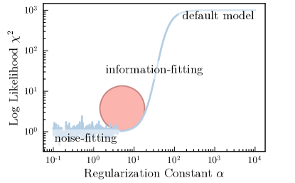
Figure 1: A schematic representation of the method to determine the optimal regularization constant when using the maximum entropy approach. The noise-fitting region is characterized by little to no change in the recovered spectra with changes to $\alpha$ and is dominated by fitting to the noise in the intermediate scattering function. The information-fitting region corresponds to spectra with deviations from the default model strongly affected by $\alpha$. The default model region consists of spectra with little or no deviation from the default model. An example of a circle fit to the data is shown in red, where an estimate of curvature can be made made from the radius.

A schematic representation of their approach is shown in Figure 1 where a sweep over possible $\alpha$ is performed with the optimal value chosen by computing the curvature of $\log_{10}\chi^{2}$ as a function of $\log_{10}\alpha$. Curvature is estimated as $\kappa=\frac{1}{R}$ where $R$ is the radius of a circle fit to the data. Three distinct regions are observed: noise-fitting, information-fitting, and default model region. The $\alpha$ value corresponding to the maximum curvature close to the noise-fitting region is the value that recovers the optimal spectral function.

The default model $D(\omega)$ was chosen to be a single Gaussian-like peak in the positive frequency space using Eq. (10) for an equally spaced frequency partition of size $N=129$ ranging from $\omega_{0}=0.0\,$\mathrm{K}\text{/}$$ to $\omega_{N}=64.0\,$\mathrm{K}\text{/}$$. For each model per simulated spectra, the parameter $\mu$ was chosen to be the first moment as calculated by Eq. (15) and the parameter:

$$\sigma=\frac{\mathrm{min}\quantity(\expectationvalue{\omega^{1}}-\omega_{0},\,\omega_{N}-\expectationvalue{\omega^{1}})}{3}.$$ (24)

where the denominator allows for sufficient damping of the default model before reaching the edges of the frequency search space. The initial guess for $S({\bf\it q},\omega)$ for each MEM simulation was set to the default model. The regularization constant $\alpha$ was swept over for an equally spaced partition in $\log_{10}$-space of size $N_{\alpha}=1001$ from $10^{-1}$ to $10^{4}$. Optimal final spectra at each error level for the data set described by Table 1 were determined as described above.

III.2 Fast and Efficient Stochastic Optimization Method

The fast and efficient stochastic optimization method (FESOM) Bao et al. (2016) is a state-of-the-art technique to determine spectral functions from imaginary time quantum Monte Carlo data. The approach uses minimal prior information by solely optimizing the likelihood function. This is achieved by brute force minimization of Eq. (19) through a numerical algorithm (described below) to within an acceptable tolerance level $\eta$. Several FESOM simulations are performed and the final spectrum is determined by averaging the results. A confidence band can be constructed by taking the standard deviation. This treatment of the final spectrum is statistically allowable since each realization has the same posterior probability when $\chi^{2}=\eta$.

In practice, a FESOM simulation is performed as follows. An initial spectrum is generated on a discretized frequency space $\{\omega_{0}\leq\omega_{1}\leq\ldots\leq\omega_{i}\leq\ldots\leq\omega_{N-1}\leq\omega_{N}\}$ obeying the normalization condition Eq. (7). The quality of fit $\chi^{2}$ is calculated via Eq. (19). For each iteration, an update to the spectrum is proposed by scaling each spectral weight $S({\bf\it q},\omega_{i})$ by $\lvert 1+x_{i}\rvert$ where $x_{i}\in\mathcal{N}(0,1)$ and normalizing by the static structure factor $S({\bf\it q})$. If the new spectrum has a $\chi^{2}$ value that is smaller than the previous iteration, the update is accepted. Iterations are performed until acceptable tolerance is achieved as described previously. In our simulations, the initial spectrum was generated using the same method described for the default model above in SectionIII.1 with the exception that the frequency space partition size was $N=513$. For each error level, $N_{R}=1000$ reconstructions of the spectral function were measured using FESOM to an acceptable tolerance level of $\eta=5\epsilon$. A maximum of $N_{I}=10^{7}$ iterations were performed for each simulation. The results were averaged to generate a final spectrum at each error level for the data set described by Table 1. The final spectra were smoothed by averaging the spectral weight in adjacent frequency bins.

IV Differential Evolution for Analytic Continuation

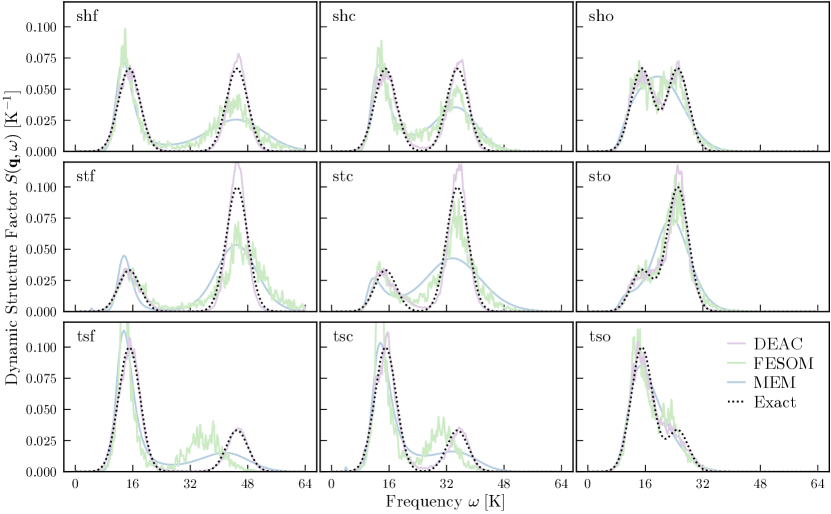
Figure 2: Nine different spectral reconstructions using different analytic continuation methods on simulated quantum Monte Carlo data. The black dashed line is the exact spectra. Results are shown for the smallest error level explored $\epsilon=0.0001$. The DEAC algorithm accurately captures the spectral features in all cases explored.

Inspired by the genetic inversion via falsification of theories (GIFT) algorithm Bertaina et al. (2017); Vitali et al. (2010), we developed an approach using evolutionary computation, the differential evolution for analytic continuation (DEAC) method that does not rely on hyperparameters. A comparison of GIFT with MEM at $T=0\;$\mathrm{K}\text{/}$$ can be found in Ref. Kora and Boninsegni (2018). The new approach developed here expands to the more difficult finite temperature regime and uses an evolutionary computation method well suited for a genome consisting of real valued numbers.

Differential evolution Storn and Price (1997) is a class of evolutionary algorithms, which determines an optimal solution within a certain tolerance based on fitness criteria. A population of candidate solutions is maintained and updated through a simple vector process described below. As the simulation progresses, each candidate solution is rated and added to the population based on some fitness criteria and the average fitness of the population improves. Here, the population is comprised of spectral functions $S({\bf\it q},\omega)$ discretized over a fixed frequency space, and the fitness of candidate solutions was calculated via Eq. (19).

Each iteration of the DEAC algorithm generates a new candidate population by the following process. For each agent $\tilde{S}_{m}({\bf\it q},\omega)$ in the population, three other agents $\tilde{S}_{j}$, $\tilde{S}_{k}$, and $\tilde{S}_{l}$ are randomly chosen such that $\tilde{S}_{m}\neq\tilde{S}_{j}\neq\tilde{S}_{k}\neq\tilde{S}_{l}$. A potential new member $\tilde{S}_{n}$ is created by iterating over the frequency space $\{\omega_{0},\ldots,\omega_{N}\}$ and for each $\omega_{i}$

$$\tilde{S}_{n}(\omega_{i})=\begin{cases}\tilde{S}_{j}(\omega_{i})+\gamma[\tilde{S}_{k}(\omega_{i})-\tilde{S}_{l}(\omega_{i})],&\mathcal{U}(0,1)\leq P^{c}\\ \tilde{S}_{m}(\omega_{i}),&\text{otherwise}\end{cases}$$ (25)

where $\mathcal{U}(0,1)$ is a random number drawn from the standard uniform distribution, $P^{c}$ is the crossover probability, and $\gamma$ is the differential weight. The new agent $\tilde{S}_{n}$ replaces $\tilde{S}_{m}$ in the next generation if fitness improves over $\tilde{S}_{m}$, otherwise $\tilde{S}_{m}$ is retained.

In a standard differential evolution simulation, the differential weight and the crossover probability would need to be optimized, and while in principle they should not affect the final outcome, in practice, a poor choice can affect convergence. Here we employ a self adaptive approach Qin and Suganthan (2005); Fan and Zhang (2016) by embedding $\gamma$ and $P_{c}$ within the genome of the candidate solutions, such that each $\tilde{S}_{m}$ has a corresponding $P^{c}_{m}$ and $\gamma_{m}$. Updates to the crossover probability are performed 10% of the time by

$$P^{c}_{n}=\begin{cases}\mathcal{U}(0,1),&\mathcal{U}(0,1)\leq 0.1\\ P^{c}_{m},&\text{otherwise}\end{cases}$$ (26)

and updates to the differential weight are also performed 10% of the time by

$$\gamma_{n}=\begin{cases}\mathcal{U}(0,2),&\mathcal{U}(0,1)\leq 0.1\\ \gamma_{m},&\text{otherwise}\end{cases}\,.$$ (27)

Note that the control parameters are updated before generating a new candidate population and $P^{c}_{n}$ and $\gamma_{n}$ should be used in Eq. (25). This ensures that beneficial changes to the crossover probability or differential weight are preserved.

The population size $N_{P}$ can be as small as $N_{P}=4$ and as large as the computing resource can manage. An optimal solution can be reached for any $N_{P}\geq 4$, although scaling of $N_{P}$ can help determine a population size that conforms to system constraints and an acceptable usage of CPU hours. Here we use $N_{P}=16$ for the simulated data, and $N_{P}=8$ for the bulk helium data.

A maximum of $N_{I}=10^{7}$ iterations were performed, where the average fitness of the candidate solution population improved with each generation. Once an individual solution $\tilde{S}_{m}({\bf\it q},\omega)$ reaches an acceptable tolerance level $\chi^{2}=\eta$, the simulation is terminated and the solution returned as the optimal spectra $S({\bf\it q},\omega)$. The tolerance levels were chosen to be the same as those used in FESOM (Section III.2) for the simulated data, and $\eta=1.0$ for superfluid helium. The frequency space partition size was $N=513$ and ranged from $\omega_{0}=0.0\,$\mathrm{K}\text{/}$$ to $\omega_{N}=64.0\,$\mathrm{K}\text{/}$$ for the simulated data, and $N=4096$ ranging from $\omega_{0}=0.0\,$\mathrm{K}\text{/}$$ to $\omega_{N}=512.0\,$\mathrm{K}\text{/}$$ for helium. In each case, $N_{R}=1000$ reconstructions of the spectral function were measured. The results were averaged to generate a final spectrum at each error level for the data set described by Table 1 and for each wave vector examined for the helium. The final spectra were smoothed by averaging the spectral weight in adjacent frequency bins. Similar to FESOM, confidence bands can be generated by taking the standard deviation.

V Results

V.1 Benchmarking on Simulated Data

Reconstructed spectra found using DEAC, MEM, and FESOM on simulated quantum Monte Carlo data are shown in Figure 2 for the small error level, $\epsilon=0.0001$. The DEAC algorithm achieves improved spectral feature resolution over the other two methods in all cases. These improvements can be seen in the goodness of fit calculated as the lack-of-fit sum of squares

$$\varphi_{\mathrm{lof}}=\frac{1}{N}\sum_{i}^{N}(S({\bf\it q},\omega_{i})-S_{\mathrm{exact}}({\bf\it q},\omega_{i}))^{2}$$ (28)

where squared deviations of the spectral weight at each frequency are averaged. Across the range of sample data, DEAC achieves the best score (where lower is better) for all nine benchmarks except in the tso case for medium error. DEAC shows almost an order of magnitude of improvement in the goodness of fit over the other two methods at small error as shown in Table 2 and half that at other error levels.

	small			medium			large
Alias	D	F	M	D	F	M	D	F	M
shf	5.30	3.95	3.75	4.66	3.93	4.19	4.17	3.91	3.57
shc	5.09	3.99	3.89	4.47	4.00	3.76	4.23	3.97	3.78
sho	4.90	4.46	4.12	4.58	4.49	4.19	4.51	4.44	3.69
stf	4.86	3.66	3.74	5.17	3.65	3.23	4.94	3.64	3.19
stc	4.73	4.03	3.51	4.98	4.03	3.48	4.79	3.94	3.46
sto	4.67	4.53	4.02	4.57	4.48	4.23	4.83	4.51	4.03
tsf	4.89	3.44	3.92	4.76	3.45	4.04	3.93	3.44	3.27
tsc	5.12	3.63	4.09	4.31	3.63	4.13	4.06	3.62	3.48
tso	4.69	4.23	4.47	4.21	4.20	4.50	4.48	4.12	4.22

Table 2: Logarithmically scaled goodness of fit for each spectral function reconstruction at each error level. Values shown are $-\log_{10}(\varphi_{\mathrm{lof}})$ where $\varphi_{\mathrm{lof}}$ is calculated by Eq. (28). More positive values indicate better qualities of fit. Here we abbreviate the methods DEAC, FESOM, and MEM as D, F, and M respectively.

A closer look at the outlier as shown in Figure 3 reveals that although MEM has a better goodness of fit, it lacks the ability to resolve two distinct peaks. Both FESOM and DEAC indicate a shoulder of a smaller peak next to the main spectral feature and encourage further QMC data collection to reduce the error level and achieve better spectral resolution. The perhaps more surprising result is MEM not winning across all the close cases as the method we employed included prior knowledge by including the first moment as a part of the default spectrum.

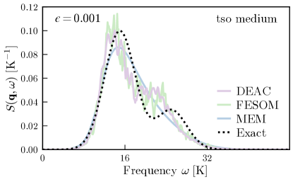
Figure 3: Analytic continuation results using DEAC, FESOM, and MEM for the tso case at medium error level. In this case, MEM achieves a better goodness of fit over FESOM and DEAC. The striking lack or even hint of two spectral peaks for the MEM results is reason to judge the FESOM and DEAC results as qualitatively better.

Another important factor is the computational efficiency of algorithms, as often spectra must be generated for a large number of ${\bf\it q}$ values. The total CPU time to achieve the final spectra for the large error data set $\epsilon=0.01$ is shown in Figure 4. These timings include the full parameter sweep for the MEM method and the $N_{R}=1000$ reconstructions for the FESOM and DEAC methods. They do not include the time needed to generate the final spectra using the curvature technique for MEM or averaging the spectra for DEAC and FESOM (as these contributions were negligible). The MEM results used up to $66\times$ ($14\times$ on average across all benchmarks) more CPU hours than DEAC, and the FESOM results used up to $79\times$ ($13\times$ on average across all benchmarks) more CPU hours than DEAC.

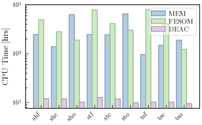
Figure 4: CPU time required to generate the final spectra using each analytic continuation technique. Timings displayed are for the largest error level explored $\epsilon=0.01$. Lower is better, and significant improvement in CPU time can be achieved using DEAC. Almost two orders of magnitude improvement can be seen over the other methods.

V.2 Bulk Helium

To test the performance of our parameter free algorithm in an experimentally relevant setting, we consider the well known phonon-roton spectrum of ⁴He at $T=1.35\,$\mathrm{K}\text{/}$$. The imaginary time scattering function was generated from canonical quantum Monte Carlo as described in Section II.3. The resulting spectrum in Figure 5 is consistent with experimental results Glyde (2017); Donnelly and Barenghi (1998); Godfrin et al. (2021); Beauvois et al. (2018); Prisk (2021), and we note it involves no adjustable parameters. Spectral peaks in the maxon and roton regions are found at momenta $q\approx 1.1\,$$$ and $q\approx 2.0\,$$$ with energy transfers of $\omega\approx 1.2\,$\mathrm{meV}\text{/}$$ and $\omega\approx 0.8\,$\mathrm{meV}\text{/}$$ respectively. Parts of the linear dispersing branch are observable, but obscured due to vertical gaps in the spectral data from certain momenta not being measured. This was either from being incommensurate with periodic boundary conditions or finite size effects.

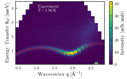
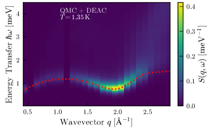
Figure 5: The phonon-roton spectrum of ⁴He at $T=1.56\,$\mathrm{K}\text{/}$$ from neutron scattering experiments on superfluid helium (top) Prisk (2021) and at $T=1.35\,$\mathrm{K}\text{/}$$ as generated by DEAC from canonical quantum Monte Carlo data (bottom). Peak locations for experimental measurements of helium at temperatures below the superfluid transition temperature $T_{\lambda}$ and saturated vapor pressure are shown as the red dashed line using splines from Donnelly and Barenghi Donnelly and Barenghi (1998). Good agreement is observed for the maxon and roton locations. Deviations from the experimental spectra and gaps in data are due to finite size effects.

Many attempts have been performed to resolve this spectra where much of the focus has been on a few fixed $q$-values Boninsegni and Ceperley (1996); Kora and Boninsegni (2018); Vitali et al. (2010); Ferré and Boronat (2016).

An advantage that DEAC and FESOM have over other methods is the ability to estimate confidence bands on spectral features. For each $N_{R}$ reconstruction of the spectrum, we determined the location of the maxima in frequency space and binned the results for each wavevector ${\bf\it q}$ investigated. Then the average and standard error were calculated in the usual way from the binned data. In Figure 6, we show the average maximum peak locations of the helium dispersion as determined using standard techniques from the average data including standard error, where the error bars indicate the full width half maximum.

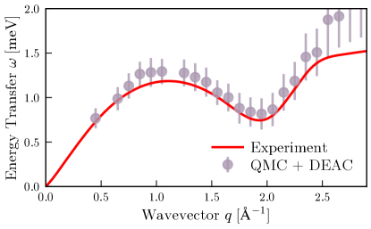
Figure 6: Maximum peak locations for the ⁴He dispersion at $T=1.35\,$\mathrm{K}\text{/}$$ as generated by analytic continuation of QMC data using the DEAC algorithm. Experimental data for low temperature helium $T<2.17\,$\mathrm{K}\text{/}$$ at saturated vapor pressure is shown Donnelly and Barenghi (1998). Again, deviations from the experimental data are observed due to finite size effects.

VI Discussion

The maximum entropy (MEM) approach is well supported in the literature and performs well for resolving spectral features for well separated peak locations. However, for closely spaced peaks, it tends to average out the resulting spectra. This effect can be seen in the overlapping cases in Figure 2. Also, for the other non-overlapping cases, there appears to be some skew in the first peak and large broadening of the second peak.

The fast and efficient stochastic optimization approach (FESOM) Bao et al. (2016) was able to resolve spectral features in all cases, but had difficulty in determining the second peak location for the tall short benchmark. This method was prone to becoming stuck in local optima and not reaching the selected tolerance level before the maximum number of iterations. For this reason and for a fairer comparison between the three methods, the timing results shown are for the large error cases where all runs were able to achieve convergence within the set tolerance. Broadening of the second peak was also an issue for this method.

The differential evolution for analytic continuation (DEAC) algorithm introduced here provided the best results in the shortest amount of CPU time in all cases tested. Proof of principle for the ability of this new method to produce experimentally relevant spectra is shown by the bulk ⁴He spectrum in Figure 5. The observed finite size effects can be mitigated by larger simulation size.

The benchmark spectra were generated using versions of DEAC, FESOM, and MEM that utilize multithreading, and were written in Julia with source code available online Nichols (2021b, c, d). Additionally, the bulk helium spectrum was generated by a C++ version of DEAC with optional GPU acceleration (both HIP and CUDA supported) with source code also available online Nichols (2021e). The authors recommend the C++ version of DEAC over the Julia version.

A note of caution is offered for using any of the three methods described above. We noticed while exploring the analytic continuation problem that spectral weight will build up in the final frequency bin if a large enough maximum frequency is not explored. For the benchmark data, this resulted in the second peak being pushed to lower energies. This problem is solved by increasing the maximum frequency at the expense of either CPU time or frequency resolution $\Delta\omega$.

In conclusion, a fast, accurate, and parameter-free method to reconstruct the dynamic structure factor from imaginary time pair correlation functions has been developed. The differential evolution for analytic continuation algorithm uses evolutionary computation with a self adaptive approach to tackle this long standing problem in many-body physics. Benchmarks on finite temperature simulated quantum Monte Carlo data against the traditional maximum entropy method and the state-of-the-art fast and efficient stochastic optimization method have shown several advantages. These are found in massive speedups and the increased fidelity of resulting spectra. The greater ability to resolve spectral features coupled with reduced computational overhead offers further opportunity to compare the stochastically exact results from quantum Monte Carlo with experimental data obtained on the real frequency axis.

VII Acknowledgments

We benefited from discussion with H. Barghathi. This research was supported in part by the National Science Foundation (NSF) under award Nos. DMR-1809027 and DMR-1808440. Computations were performed on the Vermont Advanced Computing Core supported in part by NSF award No. OAC-1827314. This work used the Extreme Science and Engineering Discovery Environment (XSEDE) Towns et al. (2014), which is supported by NSF grant number ACI-1548562. XSEDE resources used include Bridges and Bridges-2 at Pittsburgh Supercomputing Center, Comet at San Diego Supercomputer Center, and Open Science Grid (OSG) Pordes et al. (2007); Sfiligoi et al. (2009) through allocations TG-DMR190045 and TG-DMR190101. OSG is supported by the NSF under award No. 1148698, and the U.S. Department of Energy’s Office of Science.

References

- Pathria and Beale (2022) R. Pathria and P. D. Beale, “15 - Fluctuations and nonequilibrium statistical mechanics,” in Statistical Mechanics (Fourth Edition), edited by R. Pathria and P. D. Beale (Academic Press, 2022) fourth edition ed., pp. 599–657.
- Ghanem and Koch (2020) K. Ghanem and E. Koch, “Average spectrum method for analytic continuation: Efficient blocked-mode sampling and dependence on the discretization grid,” Phys. Rev. B 101, 085111 (2020).
- Goulko et al. (2017) O. Goulko, A. S. Mishchenko, L. Pollet, N. Prokof’ev, and B. Svistunov, “Numerical analytic continuation: Answers to well-posed questions,” Phys. Rev. B 95, 014102 (2017).
- Bertaina et al. (2017) G. Bertaina, D. E. Galli, and E. Vitali, “Statistical and computational intelligence approach to analytic continuation in Quantum Monte Carlo,” Adv. Phys.: X 2, 302 (2017).
- Vitali et al. (2010) E. Vitali, M. Rossi, L. Reatto, and D. E. Galli, “Ab initio low-energy dynamics of superfluid and solid 4He,” Phys. Rev. B 82, 174510 (2010).
- Jarrell and Gubernatis (1996) M. Jarrell and J. Gubernatis, “Bayesian inference and the analytic continuation of imaginary-time quantum Monte Carlo data,” Phys. Rep. 269, 133 (1996).
- Bao et al. (2016) F. Bao, Y. Tang, M. Summers, G. Zhang, C. Webster, V. Scarola, and T. A. Maier, “Fast and efficient stochastic optimization for analytic continuation,” Phys. Rev. B 94, 125149 (2016).
- Fournier et al. (2020) R. Fournier, L. Wang, O. V. Yazyev, and Q. Wu, “Artificial Neural Network Approach to the Analytic Continuation Problem,” Phys. Rev. Lett. 124, 056401 (2020).
- Raghavan et al. (2021) K. Raghavan, P. Balaprakash, A. Lovato, N. Rocco, and S. M. Wild, “Machine-learning-based inversion of nuclear responses,” Phys. Rev. C 103, 035502 (2021).
- Kades et al. (2020) L. Kades, J. M. Pawlowski, A. Rothkopf, M. Scherzer, J. M. Urban, S. J. Wetzel, N. Wink, and F. P. G. Ziegler, “Spectral reconstruction with deep neural networks,” Phys. Rev. D 102, 096001 (2020).
- Nichols (2021a) N. S. Nichols, “Available Online,” DEAC Paper Code Repository (2021a), 10.5281/zenodo.5835340, https://github.com/DelMaestroGroup/papers-code-DEAC.
- Allen and Tildesley (2017) M. P. Allen and D. J. Tildesley, Computer Simulation of Liquids: Second Edition, 2nd ed. (Oxford University Press, Oxford, 2017) p. 640.
- Villamaina and Trizac (2014) D. Villamaina and E. Trizac, “Thinking outside the box: fluctuations and finite size effects,” Eur. J. Phys. 35, 035011 (2014).
- Sturm (1993) K. Sturm, “Dynamic Structure Factor: An Introduction,” Zeitschrift fü Naturforschung A 48, 233 (1993).
- Pines and Woo (1970) D. Pines and C.-W. Woo, “Sum Rules, Structure Factors, and Phonon Dispersion in Liquid at Long Wavelengths and Low Temperatures,” Phys. Rev. Lett. 24, 1044 (1970).
- Miller et al. (1962) A. Miller, D. Pines, and P. Nozières, “Elementary Excitations in Liquid Helium,” Phys. Rev. 127, 1452 (1962).
- Groth et al. (2019) S. Groth, T. Dornheim, and J. Vorberger, “Ab initio path integral Monte Carlo approach to the static and dynamic density response of the uniform electron gas,” Phys. Rev. B 99, 235122 (2019).
- Puff (1965) R. D. Puff, “Application of Sum Rules to the Low-Temperature Interacting Boson System,” Phys. Rev. 137, A406 (1965).
- Mihara and Puff (1968) N. Mihara and R. D. Puff, “Liquid Structure Factor of Ground-State ,” Phys. Rev. 174, 221 (1968).
- Iwamoto (1986) N. Iwamoto, “Inequalities for frequency-moment sum rules of electron liquids,” Phys. Rev. A 33, 1940 (1986).
- Iwamoto et al. (1984) N. Iwamoto, E. Krotscheck, and D. Pines, “Theory of electron liquids. II. Static and dynamic form factors, correlation energy, and plasmon dispersion,” Phys. Rev. B 29, 3936 (1984).
- Boninsegni and Ceperley (1996) M. Boninsegni and D. M. Ceperley, “Density fluctuations in liquid4He. Path integrals and maximum entropy,” Journal of Low Temperature Physics 104, 339 (1996).
- Glyde (2017) H. R. Glyde, “Excitations in the quantum liquid 4He: A review,” Rep. Prog. Phys. 81, 014501 (2017).
- Feynman (1955) R. Feynman, “Chapter II Application of Quantum Mechanics to Liquid Helium,” (Elsevier, 1955) pp. 17–53.
- Pines (2018) D. Pines, Theory Of Quantum Liquids: Normal Fermi Liquids (CRC Press, 2018).
- Nozieres (2018) P. Nozieres, Theory Of Quantum Liquids: Superfluid Bose Liquids (CRC Press, 2018).
- Del Maestro (2020) A. Del Maestro, “Available Online,” Del Maestro Group Code Repository (2020).
- Herdman et al. (2014) C. M. Herdman, A. Rommal, and A. Del Maestro, “Quantum Monte Carlo measurement of the chemical potential of 4He,” Phys. Rev. B 89, 224502 (2014).
- Aziz et al. (1979) R. A. Aziz, V. P. S. Nain, J. S. Carley, W. L. Taylor, and G. T. McConville, “An accurate intermolecular potential for helium,” The Journal of Chemical Physics 70, 4330 (1979).
- Bergeron and Tremblay (2016) D. Bergeron and A.-M. S. Tremblay, “Algorithms for optimized maximum entropy and diagnostic tools for analytic continuation,” Phys. Rev. E 94, 023303 (2016).
- Malouf (2002) R. Malouf, “A Comparison of Algorithms for Maximum Entropy Parameter Estimation,” in Proceedings of the 6th Conference on Natural Language Learning - Volume 20, COLING-02 (Association for Computational Linguistics, USA, 2002) p. 1–7.
- Andrew and Gao (2007) G. Andrew and J. Gao, “Scalable Training of L1-Regularized Log-Linear Models,” in Proceedings of the 24th International Conference on Machine Learning, ICML ’07 (Association for Computing Machinery, New York, NY, USA, 2007) p. 33–40.
- Kora and Boninsegni (2018) Y. Kora and M. Boninsegni, “Dynamic structure factor of superfluid from quantum Monte Carlo: Maximum entropy revisited,” Phys. Rev. B 98, 134509 (2018).
- Storn and Price (1997) R. Storn and K. Price, “Differential Evolution – A Simple and Efficient Heuristic for global Optimization over Continuous Spaces,” Journal of Global Optimization 11, 341 (1997).
- Qin and Suganthan (2005) A. K. Qin and P. N. Suganthan, “Self-adaptive differential evolution algorithm for numerical optimization,” in 2005 IEEE Congress on Evolutionary Computation, Vol. 2 (2005) pp. 1785–1791.
- Fan and Zhang (2016) Q. Fan and Y. Zhang, “Self-adaptive differential evolution algorithm with crossover strategies adaptation and its application in parameter estimation,” Chemom. Intell. Lab. Syst. 151, 164 (2016).
- Donnelly and Barenghi (1998) R. J. Donnelly and C. F. Barenghi, “The Observed Properties of Liquid Helium at the Saturated Vapor Pressure,” Journal of Physical and Chemical Reference Data 27, 1217 (1998).
- Godfrin et al. (2021) H. Godfrin, K. Beauvois, A. Sultan, E. Krotscheck, J. Dawidowski, B. Fåk, and J. Ollivier, “Dispersion relation of Landau elementary excitations and thermodynamic properties of superfluid ,” Phys. Rev. B 103, 104516 (2021).
- Beauvois et al. (2018) K. Beauvois, J. Dawidowski, B. Fåk, H. Godfrin, E. Krotscheck, J. Ollivier, and A. Sultan, “Microscopic dynamics of superfluid : A comprehensive study by inelastic neutron scattering,” Phys. Rev. B 97, 184520 (2018).
- Prisk (2021) T. R. Prisk, (2021), Private communication.
- Ferré and Boronat (2016) G. Ferré and J. Boronat, “Dynamic structure factor of liquid across the normal-superfluid transition,” Phys. Rev. B 93, 104510 (2016).
- Nichols (2021b) N. S. Nichols, “Available Online,” DEAC.jl Julia Code Repository (2021b), https://github.com/nscottnichols/DEAC.jl.
- Nichols (2021c) N. S. Nichols, “Available Online,” FESOM.jl Julia Code Repository (2021c), https://github.com/nscottnichols/FESOM.jl.
- Nichols (2021d) N. S. Nichols, “Available Online,” MAXENT.jl Julia Code Repository (2021d), https://github.com/nscottnichols/FESOM.jl.
- Nichols (2021e) N. S. Nichols, “Available online,” DEAC C++ Code Repository (2021e), https://github.com/nscottnichols/deac-cpp.
- Towns et al. (2014) J. Towns, T. Cockerill, M. Dahan, I. Foster, K. Gaither, A. Grimshaw, V. Hazlewood, S. Lathrop, D. Lifka, G. D. Peterson, R. Roskies, J. Scott, and N. Wilkins-Diehr, “XSEDE: Accelerating Scientific Discovery,” Comput. Sci. Eng. 16, 62 (2014).
- Pordes et al. (2007) R. Pordes, D. Petravick, B. Kramer, D. Olson, M. Livny, A. Roy, P. Avery, K. Blackburn, T. Wenaus, F. Würthwein, I. Foster, R. Gardner, M. Wilde, A. Blatecky, J. McGee, and R. Quick, “The open science grid,” J. Phys.: Conf. Ser. 78, 012057 (2007).
- Sfiligoi et al. (2009) I. Sfiligoi, D. C. Bradley, B. Holzman, P. Mhashilkar, S. Padhi, and F. Wurthwein, “The Pilot Way to Grid Resources Using glideinWMS,” in 2009 WRI World Congress on Computer Science and Information Engineering, Vol. 2 (2009) p. 428.