A Parameter Space Exploration of High Resolution Numerically Evolved Early Type
Galaxies Including AGN Feedback and Accurate Dynamical Treatment of Stellar Orbits

Abstract

An extensive exploration of the model parameter space of axisymmetric Early-Type Galaxies (ETGs) hosting a central supermassive Black Hole (SMBH) is conducted by means of high resolution hydrodynamical simulations performed with our code MACER. Global properties such as 1) total SMBH accreted mass, 2) final X-ray luminosity and temperature of the X-ray emitting halos, 3) total amount of new stars formed from the cooling gas, 4) total ejected mass in form of supernovae and AGN feedback induced galactic winds, are obtained as a function of galaxy structure and internal dynamics. In addition to the galactic dark matter halo, the model galaxies are also embedded in a group/cluster dark matter halo; finally cosmological accretion is also included, with amount and time dependence derived from cosmological simulations. Angular momentum conservation leads to the formation of cold HI disks; these disks further evolve under the action of star formation induced by disk instabilities, of the associated mass discharge onto the central SMBH, and of the consequent AGN feedback. At the end of the simulations, the hot (metal enriched) gas mass is roughly $10\%$ the mass in the old stars, with twice as much having been ejected into the intergalactic medium. The cold gas disks are a $\approx$ kpc in size, and the metal rich new stars are in $0.1$ kpc disks. The masses of cold gas and new stars are roughly $0.1\%$ the mass of the old stars. Overall, the final systems appear to reproduce quite successfully the main global properties of real ETGs.

1. Introduction

Numerous observational, numerical, and theoretical studies show that in Early Type Galaxies (hereafter ETGs), the evolution of their hot X-ray emitting atmospheres (e.g., Kim et al. 2019, Babyk et al. 2018) is determined by the complex interplay between the ISM (produced by stellar mass losses and cosmological accretion from group/cluster environment), and the internal structure and dynamics of the host galaxies, the SNIa’s heating, the central SMBH AGN feedback effects (see for reviews Kim and Pellegrini 2012, Mathews and Brighenti 2003, Werner et al. 2019). Over the years, increasingly detailed and realistic simulations have been developed and performed by several groups, with specific focus on the several aspects of the problem. The improvements on the input physics can be broadly summarized in four large categories: 1) galaxy structure and internal dynamics (e.g., shape and density profiles of stars and dark matter, velocity dispersion and rotational fields of the stellar component), 2) physics of the ISM (cooling and heating mechanisms, evolution of the dust and metals content of the ISM, star formation processes, instabilities), 3) central SMBH accretion and associated AGN feedback (radiative and mechanical feedback and its dependence on the local ISM properties, radiative transfer, cosmic-ray acceleration, 4) cluster/group confining and accretion effects. Recent studies of our group with the hydro code MACER (Gan et al. 2019a,b, Gan et al. 2020, hereafter G19a,b and G20, respectively, and references therein), focused mainly on point 3), with exploratory investigations of points 1) and 2), in particular concerning the effect of galaxy shape and rotation on the SMBH accretion, gas cooling, and star formation. These high-resolution axisymmetric hydrodynamical simulations have inner boundaries ranging from 2.5 pc to 20 pc to resolve the Bondi radius. And, while only performed in 2D, they greatly exceed the spatial resolution available in most cosmological simulations.

In particular, effects of galaxy shape and rotation seem to deserve special attention, motivated by observational and theoretical arguments. In fact rotating and flat ETGs are observed to host (albeit with the usual non-negligible scatter in their properties) systematically fainter and cooler X-ray emitting halos than ETGs of same optical luminosity but of rounder shape and with less ordered rotation in the stellar population (see, e.g., Eskridge et al. 1995, Juranova et al. 2020, Kim and Fabbiano 2015, Pellegrini et al. 1997, Sarzi 2013). Preliminary simulations, conducted with a different 2D code in cylindrical coordinates (Posacki et al. 2013, Negri et al. 2014a,b, Negri et al. 2015) reassuringly showed that in fact rotation can be effective in enhancing ISM instabilities and leading to the formation of cold gaseous rotating disks, with substantial reduction of X-ray luminosity, and lower emission temperatures of the ISM (see also Brighenti and Mathews 1996, 1997; D’Ercole and Ciotti 1998, and references therein). These simulations, while modeling star formation in the equatorial gaseous disk by using a simple, physically based recipe for star formation, lacked however the modeling of angular momentum transport, with the consequent inability to properly model SMBH accretion, so that in these preliminary simulations AGN feedback was not activated. A step forward in the modeling, also including physically appropriate AGN feedback, confirming the main results of these preliminary investigations, was done in a series of subsequent papers (Ciotti et al. 2017, Pellegrini et al. 2018, Yoon et al. 2018, G20), by using galaxy models of increasing realism.

For what concerns the numerical modeling of gas flows in ETGs, two complementary approaches can be devised, each of them with its merits and limitations. In the first, one focuses on some specific, well observed galaxy, and attempts to reproduce in detail the observed features (in particular, the X-ray surface brightness profile and the the temperature profile of the ISM), to test the implemented physical assumptions. In the second, one instead considers a large set of galaxy models, spanning the range of observed galaxy properties, aiming at reproducing the observed trends of global properties, such as the ISM total X-ray luminosity and emission-weighted temperature, the final SMBH masses, the duty-cycle of the AGN, and so on. Of course, in the first approach one can use well taylored galaxy models, but the unavoidable shortcoming is that one does not have information on the specific time at which the real system is observed, a problem somewhat aggravated by the empirical (and significant) differences from system-to-system: in practice, also when modeling a well observed galaxy, from the point of view of the simulations, one is forced to interpret the results in some time-averaged way. In the second approach, one cannot expect to reproduce in great detail a single object, however global trends (presumably quite independent of very specific physical assumptions, and averaged over the large number of models) may be reproduced, thus hopefully deriving information useful to build a consistent “big picture” of the different physical mechanisms involved in the evolution of the ISM, and in the AGN feedback activity. Clearly, the exploration of the parameter space can be very time-expensive, in particular if high spatial and temporal resolution is adopted (as required for a proper numerical modeling).

In this paper we take advantage of the latest version of our high-resolution MACER code, improved in particular on the physical treatment of feedback, on the effects of rotation of the stellar component on SMBH accretion, and on star formation and disk instabilities, and we focus on the second approach, by using realistic dynamical models for the host galaxies. In particular, an extensive exploration of the model parameter space is conducted. Properties such as 1) total SMBH accreted mass, 2) final X-ray luminosity and temperature of the X-ray emitting halos, 3) total amount of new stars, 4) total ejected mass are obtained, as a function of galaxy structure (stellar and DM amount and distribution, galaxy flattening), and internal dynamics (amount of ordered rotation). A group/cluster DM halo is also added, providing an important confining effect, and finally cosmological accretion is also included, in accordance with the results of cosmological simulations (at this stage however a major omission is the neglect of the accretion of satellite galaxies). We also consider the time change of the stellar velocity dispersion and rotational velocity fields, due to mass loss of the stellar populations, and to the mass growth of the central SMBH. The code used has been developed by Ciotti & Ostriker and collaborators (2001, 2007, 2011), with recent major additions described in G19a,b and G20, to allow for the inclusion of a suite of chemical elements, and the study of dust production and destruction.

The paper is organized as follows: in Section 2 we describe the galaxy models adopted for the simulations, and in Section 3 we present the major upgrades in the input physics. Section 4 is dedicated to present the main results, while in Section 5 we discuss the results and present the conclusions, together with a list of important improvements that we are currently developing.

2. The galaxy models

A major ingredient for the hydrodynamical simulations of galactic gas flows is represented by the galaxy models hosting the flows. In fact, the models are needed in order to assign the gravitational field of the host galaxies, and the spatial and temporal distribution of the gas source terms (mass, momentum, and energy). In turn, the momentum and energy terms require the specification of the galaxy internal dynamics. Over the years, more and more realistic (and numerically tractable) models have been developed and employed in the simulations.

The galaxy models adopted here are an extension of the models already used in G19a,b and G20, and are based on the JJe dynamical models (Ciotti et al. 2021, hereafter CMPZ21). Here we recall their main structural and dynamical properties relevant for the hydrodynamical simulations. The stellar density distribution is described by an oblate ellipsoidal Jaffe (1983) model of total mass $M_{*}$, scale-length $r_{*}$, and axial ratio $0<q_{*}\leq 1$, so that its density profile is given by

$$\rho_{*}(m_{*})={M_{*}\over 4\pi q_{*}r_{*}^{3}m_{*}^{2}(1+m_{*})^{2}},\quad m_{*}^{2}\equiv{R^{2}\over r_{*}^{2}}+{z^{2}\over q_{*}^{2}r_{*}^{2}}.$$ (1)

It is useful to introduce the flattening parameter $\eta_{*}$, related to the axial ratio as $\eta_{*}=1-q_{*}$, so that $\eta_{*}=0$ corresponds to a spherical stellar distribution. The circularized effective radius $\langle R_{\rm e}\rangle$ of an ellipsoidal stellar system observed edge-on is related to the effective radius $R_{\rm e}$ of the same model in the spherical limit (or when observed face-on) by the identity

$$\langle R_{\rm e}\rangle=\sqrt{q_{*}}R_{\rm e},$$ (2)

moreover, in the edge-on projection of an ellipsoidal system, the isophotal flattening coincide with the intrinsic flattening. As is well known, the projected density profile of the Jaffe model is remarkably similar to the de Vaucouleurs $R^{1/4}$ law over a quite large radial range, and in the spherical case $R_{\rm e}\simeq 3r_{*}/4$, so that we can use Equation (2) to determine the scale $r_{*}$ for our models once $q_{*}$ and $\langle R_{\rm e}\rangle$ are fixed by observations.

In JJe models the stellar distribution is embedded in a galactic dark matter (hereafter DM) halo, so that the total (stellar plus DM) galaxy density distribution is again described by a Jaffe ellipsoidal distribution of total mass $M_{\rm g}={\cal R}M_{*}$, axial ratio $q_{\rm g}$, and scale length $r_{\rm g}=\xi r_{*}$:

$$\rho_{\rm g}(m_{\rm g})={M_{*}{\cal R}\xi\over 4\pi r_{*}^{3}q_{\rm g}m_{\rm g}^{2}(\xi+m_{\rm g})^{2}},\quad m_{\rm g}^{2}\equiv{R^{2}\over r_{*}^{2}}+{z^{2}\over q_{\rm g}^{2}r_{*}^{2}};$$ (3)

in the present models we always assume the natural choice $\xi\geq 1$. As in our previous papers in this series (G19a,b, G20), for simplicity we restrict to the case of spherically symmetric $\rho_{\rm g}$, i.e., we set $q_{\rm g}=1$ in Equation (3). The approximation is quite acceptable for moderately flattened galaxies (as the isopotential surfaces are in general rounder than the associated mass density), with the additional advantage of a simple expression for the galaxy gravitational field, and of explicit expressions for the solutions of the Jeans equations, of easy implementation in the hydrodynamical code (see Section 2.1). In the spherical limit, the total galaxy mass contained in the sphere of radius $r$, and the galaxy potential, are given by

$$M_{\rm g}(r)={M_{*}{\cal R}s\over\xi+s},\qquad\phi_{\rm g}(r)={GM_{*}{\cal R}\over r_{*}\xi}\ln{s\over\xi+s},\qquad s\equiv{r\over r_{*}}.$$ (4)

Since in JJe models $\rho_{\rm g}$ and $\rho_{*}$ are assigned, a condition for the positivity of the galaxy DM halo density distribution $\rho_{\rm DM}=\rho_{\rm g}-\rho_{*}$ is needed. From Equation (13) in CMPZ21, imposing $\xi\geq 1$ and $q_{\rm g}=1$, the positivity condition reduces to

$${\cal R}\geq{\cal R}_{\rm m}={\xi\over 1-\eta_{*}},$$ (5)

A model with ${\cal R}={\cal R}_{\rm m}$ is called minimum halo model, and it can be shown that in this case $\rho_{\rm DM}$ is well described by the NFW profile over a large radial range (see Ciotti & Ziaee Lorzad 2018; Ciotti, Mancino and Pellegrini 2019, CMPZ21), for this reason in the simulations we set the initial galaxy parameters to the minimum-halo case. Notice that the total (stars plus DM) galaxy density profile$\rho_{\rm g}$ in Equation (3) is proportional to $r^{-2}$ inside $r_{\rm g}$: this property is one of the motivations behind the construction of JJe models, as different theoretical and observational findings support this assumption over a large radial range (e.g., see among others, Wang et al. 2019, 2020; Li, Shu and Wang 2018; Cappellari et al. 2015; Poci, Cappellari and McDermid 2017; Lyskova, Churazov and Naab 2018; Auger et al. 2010; Barnabè et al. 2011; Koopmans et al. 2009; Gavazzi et al. 2007; Serra et al. 2016; Bellstedt et al. 2018).

In order to take into account the effects of a group/cluster DM halo on the gas flows, we also consider the gravitational field produced by a spherically symmetric quasi-isothermal DM halo of asymptotic circular velocity $v_{\rm h}$ and scale-length $r_{\rm h}=\xi_{\rm h}r_{*}$

$$\rho_{\rm h}(r)={v_{\rm h}^{2}\over 4\pi Gr_{*}^{2}(\xi_{\rm h}^{2}+s^{2})},$$ (6)

$$M_{\rm h}(r)={v_{\rm h}^{2}r_{*}\over G}\,\left(s-\xi_{\rm h}\arctan{s\over\xi_{\rm h}}\right),\qquad\phi_{\rm h}(r)=v_{\rm h}^{2}\,\left(\ln{\sqrt{1+s^{2}/\xi_{\rm h}^{2}}\over{\rm e}}+{\xi_{\rm h}\over s}\arctan{s\over\xi_{\rm h}}\right).$$ (7)

Notice that in Equations (4) and (7) we fixed $\phi_{\rm g}(\infty)=0=\phi_{\rm h}(0)$. In the simulations we consider models with $\xi_{\rm h}\gg 1$, and so, as we will see in the next Section, the group/cluster DM component does not alter significantly the internal dynamics of the models (see Section 2.1).

The stellar mass $\langle M_{*}\rangle(r)$ contained in a sphere of radius $r$ centered in the origin is easily computed in the homeoidal expansion approximation, and from Equations (15)-(16) in CMPZ21 we have

$$\langle M_{*}\rangle(r)={M_{*}s\over 1+s}\left[1+{\eta_{*}\over 3(1+s)}\right],$$ (8)

so that the total DM mass (galactic plus group/cluster) inside the same sphere is

$$M_{\rm DM}(r)={M_{*}{\cal R}s\over\xi+s}-\langle M_{*}\rangle(r)+M_{\rm h}(r).$$ (9)

For the three families of models in Table 1, it follows that $M_{\rm DM}(r)/M_{\rm g}(r)\simeq 52\%$ at $r=\langle R_{\rm e}\rangle$, and $\simeq 64\%$ at $r=2\langle R_{\rm e}\rangle$ for $\eta_{*}=0.3$, and for reference $\simeq 39\%$ at $r=R_{\rm e}$, and $\simeq 55\%$ at $r=2R_{\rm e}$, for $\eta_{*}=0$.

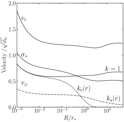
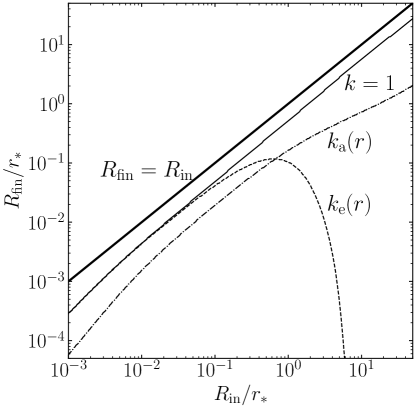
Figure 1.— Left: radial profiles of the stellar velocities in the equatorial plane in units of $\sqrt{\phi_{\rm n}}\equiv\sqrt{GM_{*}/r_{*}}$ (the numerical values of this normalization scale are given in Column (7) of Table 1 for the different model families). From top to bottom, the circular velocity $v_{\rm c}$ in Equation (17), the stellar vertical velocity dispersion component $\sigma_{*}$ in Equation (A1), and the three different azimuthal streaming velocities $\overline{v_{\varphi}}$ obtained from the first of Equations (11), respectively for the isotropic rotator (solid, $k=1$), and for the exponentially declining (dashed, $k=k_{\rm e}$) and asymptotically flat (dot-dashed, $k=k_{\rm a}$) Satoh decompositions in Equation (12). The effect of the central SMBH is clearly visibile in the innermost regions; notice also that in the exponential decomposition the stars rotate faster in the inner regions (as the isotropic rotator) than in the asymptotically flat decomposition, while rotation is the lowest in the outher galactic regions. Right: final circularization radius $R_{\rm fin}$ for the gas infalling on the equatorial plane at the radius $R_{\rm in}$, under the assumption of angular momentum conservation discussed in Section 4.2 (see in particular Equation 30). The solid line refers to isotropic rotators, the dot-dashed line to the asymptotically flat decomposition, and the dashed line to the exponential decomposition. The heavy solid line marks the locus of $R_{\rm fin}=R_{\rm in}$.

Finally, a SMBH of initial mass $M_{\rm BH}=\mu M_{*}$ (with an initial value of $\mu\simeq 10^{-3}$, half of the currently observationally estimated value) is added at the center of the galaxy, with

$$\phi_{\rm BH}(r)=-{GM_{*}\mu\over r}.$$ (10)

2.1. Internal Dynamics

The internal dynamics of the galaxy models, i.e., their velocity dispersion and ordered rotation fields, are important ingredients of the problem, as they determine the momentum and kinetic energy sources associated with stellar mass losses that enter the hydrodynamical equations. The kinematical fields are obtained by solving the Jeans Equations for the density $\rho_{*}$, under the assumption of a two-integral phase-space distribution function; here we just recall the main properties relevant for the setup of the simulations (see CMPZ21, for a complete description of the models). In particular, the Jeans equations for the stellar component are solved in homeoidal approximation, so that the solution can be expressed in fully analytical form (see Appendix A). This fact not only allows for a simple numerical implementation (G19a), but it also allows to follow the secular changes of the gravitational and kinematical fields due to the stellar mass losses and the mass growth of the central SMBH, just by imposing the required time dependence on the structural parameters (see Appendix B). We also consider the effects on the gas flows of the (time dependent) gravitational field associated with the formation of the stellar disk in the equatorial plane (Section 3), and with the gravitational field of a group/cluster DM halo; for simplicity, instead, we do not consider their effects on the stellar kinematical field, so the formulae in the Appendices give the kinematical field produced by the total mass distribution (disk excluded) and the central SMBH.

Table 1Structural properties of the three families of models

Model family	$L_{\rm B}$	$M_{*}$	$r_{*}$	$\langle R_{\rm e}\rangle$	$v_{\rm c}(0)$	$\sigma_{*}(0)$	$\sqrt{GM_{*}/r_{*}}$	$v_{\rm h}$
	$(10^{11}\,L_{\rm B,\odot})$	$(10^{11}\,{\rm M}_{\odot})$	$({\rm kpc})$	$({\rm kpc})$	$({\rm km}\;{\rm s}^{-1})$	$({\rm km}\;{\rm s}^{-1})$	$({\rm km}\;{\rm s}^{-1})$	$({\rm km}\;{\rm s}^{-1})$
	(1)	(2)	(3)	(4)	(5)	(6)	(7)	(8)
LM	$0.32$	$1.54$	$7.33$	$4.57$	$360$	$223$	$301$	$360$
MM	$0.65$	$3.35$	$11.29$	$7.04$	$427$	$265$	$357$	$427$
HM	$1.38$	$7.80$	$18.94$	$11.80$	$504$	$312$	$421$	$504$

• For the family name on the left, each column gives: (1) the galaxy luminosity in the $B$-band, (2) the initial stellar mass, (3) the scale-length of the stellar distribution (Equation 1), (4) the edge-on circularized effective radius (Equation 2), (5) the galaxy central circular velocity (in absence of the SMBH and in the minimum halo case, Equation 16), (6) the stellar central velocity dispersion (in absence of the SMBH, and in the minimum halo case, Equation 15), (7) the velocity scale of the models, and (8) the asymptotic circular velocity of the quasi-isothermal DM halo (Equation 6), fixed to coincide with $v_{\rm g}(0)$. For all models, the flattening of the stellar distribution in Equation (1) is $\eta_{*}=0.3$, the initial SMBH-to-stellar mass ratio is $\mu=M_{\rm BH}/M_{*}=0.001$, the parameters $\xi$ and ${\cal R}$ characterizing the total galaxy density in Equation (3) are $\xi=12.6$ and ${\cal R}=18$, corresponding to a minimum-halo model from Equation (5), and the scale-length of the quasi-isothermal halo in Equation (6) is $\xi_{\rm h}=5$.

As is well known, the azimuthal velocity field is split in its ordered ($\overline{v_{\varphi}}$) and dispersion ($\sigma_{\varphi}$) components by adopting a generalised Satoh (1980) $k$-decomposition

$$\overline{v_{\varphi}}=k\,\sqrt{\Delta_{*}},\qquad\sigma_{\varphi}^{2}=\sigma_{*}^{2}+(1-k^{2})\Delta_{*},\qquad\Delta_{*}=\overline{v_{\varphi}}^{2}+\sigma_{\varphi}^{2}-\sigma_{*}^{2};$$ (11)

where $\sigma_{*}$ is the vertical (and then also radial) velocity dispersion, and the explicit expressions of $\sigma_{*}$ and $\Delta_{*}$ are given in Appendix A. Therefore, $k=1$ correspond to a “fast” rotating galaxy (the isotropic rotator), while $k=0$ describes a galaxy with a flattening totally supported by tangential velocity dispersion. In addition to the standard case with constant $k$, we also explore two more families of rotating galaxies, with a spatially-dependent Satoh parameter

$$k_{\rm a}(r)=k_{0}+(k_{\infty}-k_{0}){s\over\xi_{0}+s},\qquad k_{\rm e}(r)={\rm e}^{-r/\langle R_{\rm e}\rangle},$$ (12)

with $k_{0}=0.42$, $k_{\infty}=0.05$, $\xi_{0}=2.67$. In the exponential case $\overline{v_{\varphi}}$ decreases significantly at large radii, while the $k_{\rm a}(r)$ case $\overline{v_{\varphi}}$ becomes asymptotically flat; in the central region, instead, stars of a model with $k_{\rm e}(r)$ rotate rotate almost as fast as an isotropic rotator, faster than those in the asymptotically flat case $k_{\rm a}(r)$, as at the center $k_{\rm a}(0)=k_{0}$ is lower than unity (see Fig. 1).

The assumptions of homeoidal expansion, and the neglect of the effects of the external DM halo on the stellar dynamics inside a few effective radii of the galaxy (corresponding to more than $99\%$ of the total stellar mass) was checked by numerical integration of the Jeans Equations in the full gravitational field, without using the homeoidal expansion; the integration was done with the multi-component stellar dynamical code JASMINE2 (Jeans AxiSymmetric Models of Galaxies IN Equilibrium; see Caravita et al. 2021, see also Posacki et al. 2013). We found that these effects within $\approx 2R_{\rm e}$ are in fact negligible, so that for the purposes of the present exploration the formulae in Appendix A can be safely adopted.

To set up realistic galaxy models, we recall that their stellar central velocity dispersion in absence of the central SMBH, can be obtained combining Equations (26) and (42) in CMPZ21 (the former with ${\cal R}=\xi=1$ and $\eta_{\rm g}=\eta_{*}$, and the latter with $\mu=0$ and $\eta_{\rm g}=0$):

$$\sigma_{*}^{2}(0) = {GM_{*}{\cal R}\over 2\xi r_{*}}{1-\eta_{*}\cos^{2}\theta\over 1+\eta_{*}-2\eta_{*}\cos^{2}\theta}$$ (13)

$$= {GM_{*}{\cal R}\over 2\xi(1+\eta_{*})r_{*}}={GM_{*}\over 2(1-\eta_{*}^{2})r_{*}},$$ (15)

where the second equality holds when evaluating the limit along the equatorial plane ($\theta=\pi/2$), and finally the last expression for minimum halo models, i.e. for ${\cal R}={\cal R}_{\rm m}$ given in Equation (5). We adopt $\sigma_{*}(0)$ as a proxy for the observed velocity dispersion of the galaxy in the central regions (outside the sphere of influence of the central SMBH). Moreover, from Equation (4) it follows that the circular velocity of JJe models does not vanishes at the center, and

$$v_{\rm g}^{2}(0)={GM_{*}{\cal R}\over r_{*}\xi}=2(1+\eta_{*})\sigma_{*}^{2}(0),$$ (16)

where the last expression holds independently of the minimum halo model assumption. Finally, the model circular velocity in the equatorial plane $v_{\rm c}^{2}(r)=v_{\rm BH}^{2}(r)+v_{\rm g}^{2}(r)+v_{\rm h}^{2}(r)$ can be written in terms of $v_{\rm g}(0)$ as

$${v_{\rm c}^{2}(r)\over v_{\rm g}^{2}(0)}={\mu\xi\over{\cal R}s}+{\xi\over\xi+s}+{v_{\rm h}^{2}\over v_{\rm g}^{2}(0)}\left(1-{\xi_{\rm h}\over s}\arctan{s\over\xi_{\rm h}}\right),$$ (17)

where we neglect for simplicity the contribution to the gravitational field of the equatorial stellar disk formed by the cooling and rotating ISM (see Section 3): notice that in absence of the central SMBH, $v_{\rm c}(0)=v_{\rm g}(0)$. If needed, the equation above can be recast without difficulty in terms of $\sigma_{*}(0)$, and further specialized to the minimum halo case.

3. The input physics and the hydrodynamical simulations

The hydrodynamical Equations in the simulations are given in Equations (1)-(2)-(3) in G19a, where a full discussion of the various terms is provided. Here we recall the points of direct relevance for the present paper, and in particular the changes and the additions to the input physics with respect to G19a.

The mass source terms for the galactic gas flows are provided by the mass return from stellar evolution (including mass loss of red giants and AGB stars, SNIa explosions from the passively evolving population and SNII from the new stars formed, see Appendix B in G19a, see also Pellegrini 2012, and Ciotti & Ostriker 2012), and by cosmological accretion from a circumgalactic medium (hereafter CGM). Stellar evolution injects over the galaxy body a total amount of gas of the order of $\approx 10\%$ of the initial stellar mass, with an almost power-law steadily declining injection rate $\dot{\rho}=\alpha(t)\rho_{*}$, where $\rho$ is the gas density. Instead, the time-dependence of cosmological mass accretion from the CGM is modeled following Choi et al. (2017) and Brennan et al. (2018), and according to Equation (12) of G19a is given by

$$\dot{M}_{\rm CGM}(t)=2M_{\rm acc}{{\rm e}^{-(t/t_{0})^{2}}\over 1-{\rm e}^{-(\Delta t/t_{0})^{2}}}{t\over t_{0}^{2}},$$ (18)

where we fix $t_{0}=9$ Gyr, and we scale $M_{\rm acc}$ so that the total mass accreted from the CGM is $\simeq 0.44M_{*}$ during the time span on the simulation, $\Delta t=12$ Gyr.

The various source terms are injected into the galaxy, not only mass, but also momentum, internal, and kinetic energy; the associated terms are given in Equations (52)-(53) in G19a (Negri et al. 2014a,b; Ciotti et al. 2017, see also Chapter 10 in Ciotti 2021). In particular, the dynamical properties of the stellar component enter in the thermalization term in the energy equation as

$$\dot{E}_{S}=\dot{\rho}\,{{\rm Tr}\,\sigma^{2}+\|{\bf u}-\overline{v_{\varphi}}{\bf e}_{\varphi}\|^{2}\over 2}$$ (19)

where ${\rm Tr}\,\sigma_{*}^{2}=2\sigma_{*}^{2}+\sigma_{\varphi}^{2}=3\sigma_{*}^{2}+(1-k^{2})\Delta_{*}$ is the trace of the velocity dispersion tensor, ${\bf u}$ is the fluid velocity, and $\overline{v_{\varphi}}$ the azimuthal streaming velocity of stars in Equation (11). Similarly, it can be proved that the momentum source term is given by

$$\dot{\bf m}_{S}=\dot{\rho}\,\overline{v_{\varphi}}{\bf e}_{\varphi}.$$ (20)

Also the mass accretion flow from the CGM imposed at the outer boundary of the numerical grid injects energy and momentum in the computational domain. We assume a purely radial accretion velocity at the outer grid boundary (at $r_{\rm t}=250$ kpc), so no angular momentum is associated with $\dot{M}_{\rm CGM}$, and the modulus of this infall velocity is

$$v_{\rm CGM}=\sqrt{-{\phi_{\rm g}(r_{\rm t})-v_{\rm h}^{2}(r_{\rm t})\over 2}}.$$ (21)

This value corresponds to half of the free-fall velocity from infinity, under the assumption that the DM quasi-isothermal halo in Equation (6) is truncated at $r_{\rm t}$. Besides the mass input rate and infall velocity, the numerical modeling also requires the angular distribution and the temperature of the infalling material. Following G19a, its internal energy is set so that its sound velocity equals $v_{\rm CGM}$, while the CGM mass flux is weighted by a $\sin^{2}\theta$ angular dependence, therefore most of the CGM is injected near the equatorial plane. Finally, the metallicity of the CGM is obtained by assuming $\dot{M}_{\rm CGM}$ made of $1/4$ primordial gas, and $3/4$ low metallicity gas of $0.2$ solar abundance (see also Table 1 in G19b).

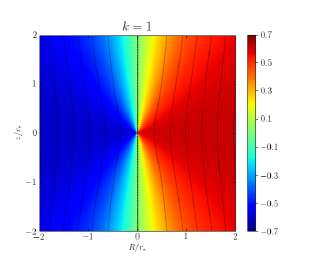
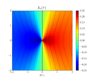
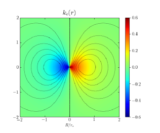
Figure 2.— Maps of the stellar ordered rotational velocity field $\overline{v_{\varphi}}/\sqrt{\phi_{\rm n}}$ in the $(R,z)$ plane, for the isotropic rotator (left), and for the two spatially dependent Satoh decompositions in Equation (12); $\phi_{\rm n}=GM_{*}/r_{*}$ is given in Table 1 for the different model families. The dotted lines are contours of constant angular momentum per unit mass of the stellar component; as shown in Equation (30), in absence of mass sources and viscous dissipation, or for a gaseous halo rotating with the same velocity $\overline{v_{\varphi}}$ of the stars, the cooling gas would fall at $R_{\rm in}$ on the equatorial plane along these lines, and then contract to $R_{\rm fin}$ as illustrated in the right panel of Figure 1.

In rotating models, we follow the evolution of the equatorial cold gaseous disk produced by the gas inflow and cooling, modeling the star formation in it, and the consequent gas accretion on the SMBH associated with the (local) Toomre instability. From Equations (13)-(14) in G19a, we evaluate at each time-step the $Q$-profile of the disk as:

$$Q(R)={c_{s}\kappa\over\pi G\Sigma},\qquad\kappa^{2}={2\Omega\over R}{d(\Omega R^{2})\over dR},\qquad\Omega(R)={v_{\rm c}(R)\over R},$$ (22)

where $\Sigma$ is the gas surface density of the disk, $c_{s}$ is the sound velocity, and $v_{\rm c}$ is the circular velocity in the equatorial plane given by Equation (17). When the Toomre instability affects (a ring) in the cold gaseous disk, we assume that a fraction $\Delta Q=\max(1-Q,0)$ of the unstable gas falls onto the center, on a time scale given by the local $v_{\rm c}(R)$ as in Equation (15) in G19a, which will result in decrement of $\Sigma$ (thus increment of $Q$). We refer to G19a also for a description of the algorithm for the numerical treatment of instability, and the associated redistribution of mass, energy, and angular momentum, as well as of the disk $\alpha$-viscosity. In this way, $Q$ is re-established to unity, and the disk self-regulates locally (Bertin and Lodato 1999, Cossins et al. 2009).

Disk instability induces also star formation, and according Equation (20) in G19a,

$$\dot{\rho}_{*,Q}=\eta_{\rm SF,Q}\,\Delta Q\,\rho\,\Omega,\qquad\Delta Q=\max(1-Q,0),\qquad\eta_{\rm SF,Q}=0.02,$$ (23)

where we reduced $\eta_{\rm SF}$ by a factor of 5 respect to the value of $0.1$ adopted in G19a. The IMF of star formed in the disk is assumed to be top-heavy (e.g., see Goodman and Tan 2004) to match the IMF seen in the central disk of MW and M31, and we assume an initial mass function for stars of mass $M$, formed in the unit time, at time $t$, of the form:

$${dN\over dM}={N_{0}(t)\over{\rm M}_{\odot}}\left({M\over{\rm M}_{\odot}}\right)^{-1.65},$$ (24)

with ${\rm M}_{\odot}<M<50{\rm M}_{\odot}$, and $N_{0}(t)$ determined to match the total mass of disk stars formed in the time step. Such an IMF gives $\approx 60\%$ of the total new star mass in massive stars ($M>8{\rm M}_{\odot}$), which will turn into SNe II on a timescale of $\approx 2\times 10^{7}$ yrs.

Disk instability is not the only channel considered for star formation. In the simulations we also allow for star formation provided that 1) the gas temperature falls below $4\times 10^{4}$ K, and 2) the gas density is higher than $10^{5}$ atom/cm^-3. When the temperature and the density of a gas element satisfy the conditions above, star formation takes place via Jeans instability with the standard timescale given by $\max(\tau_{\rm cool},\tau_{\rm dyn})$, as fully described in Equations (22)-(23) in G19a.

A new feature of the present simulations is the gravitational effect on the gas flows due to the stellar disk of new stars formed by the rotating cooling gas. In fact, albeit the total mass of the disk at any time is much lower than the total initial galaxy mass (stars plus DM), its gravitational field can be important in the central galactic region, especially near the equatorial plane. Two competitive effects of the compression produced by the vertical gravitational field of the stellar disk on the accreting gas are expected: one is compressional heating, with a reduction of accretion, the other is the tendency towards gas cooling and accretion, due to the increase in gas density. In past simulations of rotating gas flows (e.g., Negri et al. 2014a,b; Ciotti et al. 2017), only the second effect could be at work, as the gravitational field of the stellar disk was not taken into account. We consider here a semi-quantitative modelization of the disk that allows for a fast numerical computation. In practice, at each time-step, we compute the time dependent disk stellar mass $M_{\rm d*}(t)$, and the half mass disk radius $R_{\rm d*}(t)$ from the history of star formation (see Table 2), then we assume that the disk is described by a Kuzmin-Toomre razor thin disk (see Binney and Tremaine 2008)

$$\Sigma_{\rm d*}(R)={M_{\rm d*}a\over 2\pi(R^{2}+a^{2})^{3/2}},\quad\phi_{\rm d*}(R,z)=-{GM_{\rm d*}\over\sqrt{R^{2}+(a+|z|)^{2}}},$$ (25)

where $a=R_{\rm d*}/\sqrt{3}$. The formula above is used to compute and update at each time-step the vertical and radial gravitational fields produced by the stellar disk. For simplicity we do not compute the gravitational field due to the gaseous equatorial disk, nor the modifications of the stellar kinematics produced by the (time-dependent) gravitational field of the stellar disk; instead we take into account the change in the total gravitational field due to the growth of the central SMBH and the decrease of stellar mass (see Appendix B for more details).

Here we list the main additions/changes adopted in the present simulations. Following the treatment in Núñez et al. (2017), we now also consider the effect of UV heating produced by the (massive) new stars formed in the disk, updating the ISM temperature as

$${dT\over dt}={10^{4}\,{\rm K}-T\over t_{\rm rec}},\quad{\rm if}\quad T\leq 10^{4}\,{\rm K}$$ (26)

where the recombination time-scale $t_{\rm rec}$ is estimated as

$$t_{\rm rec}\equiv{1\over n_{\rm H}\alpha_{\rm B}},\quad\alpha_{\rm B}\simeq 2.56\,10^{-13}\;{\rm cm}^{-3}{\rm s}^{-1},$$ (27)

where $n_{\rm H}$ is the hydrogen number density of the ISM in cm^-3, and $\alpha_{\rm B}$ is the effective radiative recombination rate for hydrogen, assuming a gas temperature of $10^{4}$ K (Draine 2011). The UV heating is effective in each grid, provided that 1) the temperature is less than $10^{4}$ K, and 2) and the numerical grid size is smaller than the Stromgren sphere, estimated from Equation (3) of Núñez et al. (2017).

A key ingredient of the hydrodynamical simulations is represented by the input physics describing energy and momentum feedback from the stellar components, and from accretion events on the central MBH. For a complete description of the input physics and its numerical implementation we refer to Section 2.7 in G19a, and Appendix A and B therein. (1) we adopted a maximum wind efficiency of $\epsilon_{\rm w}^{\rm M}=0.005$ as in G19a, (2) we increased the opening angle of the AGN winds by weighting its angular distribution by $|\cos\theta|$ (rather than $\cos^{2}\theta$ as in G19a); and (3) we smoothed the transition from the cold to the hot AGN feedback mode by introducing two correction factors ($A=0.5$, $B=0.5$) to Equations (27) and (28) in G19a as follows:

$$\epsilon_{\rm w}=\epsilon_{\rm w}^{\rm M}\sqrt{{5\,l\over 4+l}\,{\rm e}^{-\left(A\,{\dot{M}_{\rm disk,crit}}/{\dot{M}_{\rm BH}}\right)^{4}}}$$ (28)

$$\dot{M}_{\rm w}=\dot{M}_{\rm disk}\times\left(1-B\,\sqrt{{3r_{s}\over r_{\rm tr}}}\right).$$ (29)

As a check, we performed several numerical experiments, at different spatial resolutions (up to a factor of $10$ higher), and with different choices for the parameters modeling AGN feedback/star formation/CGM accretion. In general these changes produce results in the expected direction, and overall the presented models, although can surely be improved in some specific aspect, are well representative of the results that can be obtained in the present framework.

3.1. The numerical code

We solve the Eulerian hydrodynamical equations, together with those relative to 12 metal tracers (G19b) and grain physics (G20), with our high-resolution MACER (Massive AGN Controlled Ellipticals Resolved) grid hydrodynamical code (G19a), based on the Athena++ code (version 1.0.0; Stone et al. 2020). We use spherical coordinates $(r,\theta)$ and we assume axi-symmetry, but allow for rotation (a.k.a. 2.5-dimensional simulation). The outer boundary is chosen as $250$ kpc from the galaxy center to well enclose the whole stellar distribution of the galaxy, and also a significant region of the group/cluster DM halo. The inner radial grid point $r_{\rm in}$ is placed at $25$ pc from the galaxy center, allowing us to resolve the fiducial Bondi radius; for example, the Bondi radius of the three families of models in Table 1, evaluated for a reference gas temperature of $T=10^{6}$ K, and an initial SMBH mass of $M_{\rm BH}=0.001M_{*}$, is $\simeq 30$ pc, $\simeq 65$ pc, and $\simeq 150$ pc, respectively for LM, MM, and HM models. Of course, as the SMBH mass increases with time, the numerical resolution tends to improve as the simulations proceed. Even if this resolution is quite high when compared to that adopted in other numerical studies, for some tests (see below) we also performed significantly more time-expensive simulations, with $r_{in}=2.5$ pc. The radial grid is logarithmic, with 120 grid points and an expansion factor of $\Delta r_{i+1}/\Delta r_{i}=1.1$ between two adiacent grids. The azimuthal angle $\theta$ is divided into 30 uniform cells, and covers an azimuthal range from $0.05\pi$ to $0.95\pi$. The numerical solver for the gas dynamics is composed by the combination of the HLLE Riemann Solver, the PLM reconstruction, and the second-order van Leer integrator. Outflow boundary conditions are imposed at the galaxy outskirts, which allows the gas to escape from the galaxy, but does not force it to do so. The inner boundary conditions are designed to allow for the ISM to flow inward freely, and to avoid mass outflow from the center, while the treatment of the AGN winds is implemented at the innermost active cells, placed immediately outside the inner boundary radius.

4. Exploring the parameter space: results

¿From the description of the models in Section 2 and of the input physics in Section 3, it should be clear that a systematic and complete exploration of the parameter space is impossible. In fact, a run of a model with the inner grid placed at 25 pc from the origin takes around 3-4 days with 40 cores ($2\times$ Skylake 6148 on a single node), while it takes $10\times$ longer time with the increased resolution and the first grid placed at 2.5 pc from the center. For this reason we fixed the galaxy flattening to represent E3 galaxies, and we consider three representative values for the initial stellar mass, i.e. $M_{*}=1.5\times 10^{11}{\rm M}_{\odot}$, $3.4\times 10^{11}{\rm M}_{\odot}$, and $7.8\times 10^{11}{\rm M}_{\odot}$; the explored models (respectively LM, MM, and HM in Table 1) correspond to galaxies that are massive enough that the evolution of the gaseous halo is not entirely dominated by SNIa heating (e.g., Ciotti et al. 1991), being smaller systems able to sustain galactic winds just due to the SN energy input. The models are constructed to be on the Fundamental Plane of elliptical galaxies, and as in our previous works the age of the galaxy at the beginning of the simulation is fixed to be 2 Gyr, so that the initial phases of galaxy formation are terminated (and a SMBH with a mass near to observed values is assumed to be be already in place). The galaxy DM halo corresponds to minimum halo models, with a mass 18 times larger than the initial stellar mass, and a scale length $\simeq 13$ times larger than that of the stellar distribution; in this way, the galactic DM halo is very well represented by a NFW-like profile over a very large radial range, down to the galaxy center. The group/cluster DM halo is instead important only at very large radii (outside several effective radii of the galaxy), with asymptotic circular velocity fixed to match the circular velocity near the center (in absence of central SMBH). All the structural parameters of the models are given in Table 1. Finally, as detailed in Table 2, for each of the three mass models, we consider three different rotational supports: no rotation (all the galaxy flattening is due to tangential velocity dispersion), moderate rotation (rotation exponentially declining in the outer regions as described by Equation (12)), and finally the isotropic rotator case (all the galaxy flattening is supported by ordered rotation).

Table 2Integrated properties of the models at 13.7 Gyr

Model name	$\Delta M_{\rm BH}$	$M_{\rm dHI}$	$R_{\rm dHI}$	$\langle\Sigma_{\rm dHI}\rangle$	$M_{\rm d*}$	$R_{\rm d*}$	$\Delta M_{*}$	$M_{\rm out}$	$M_{\rm hot}$	$L_{\rm X}$	$T_{\rm X}$
	$(10^{8}{\rm M}_{\odot})$	$(10^{8}{\rm M}_{\odot})$	$({\rm kpc})$	$({\rm M}_{\odot}/{\rm pc}^{2})$	$(10^{8}{\rm M}_{\odot})$	$({\rm kpc})$	$(10^{8}{\rm M}_{\odot})$	$(10^{8}{\rm M}_{\odot})$	$(10^{8}{\rm M}_{\odot})$	$(10^{40}{\rm erg}/{\rm s})$	$(10^{6}\,{\rm K})$
	(1)	(2)	(3)	(4)	(5)	(6)	(7)	(8)	(9)	(10)	(11)
LM0	7.0	0.0	0.0	-	0.0	0.0	0.0	204.5	5.6	5.4	6.1
LMk	12.8	2.4	0.7	150.3	2.1	0.1	4.8	507.1	4.3	0.8	6.9
LM1	16.7	60.3	4.4	101.4	3.0	0.3	6.8	523.0	1.6	0.1	11.0
MM0	22.2	0.0	0.0	-	0.0	0.0	0.0	156.6	49.9	20.3	10.9
MMk	36.7	11.0	0.5	1454	5.3	0.1	12.2	1181.5	21.1	8.6	9.4
MM1	71.9	46.6	3.6	114.4	12.2	0.3	28.0	1236.8	11.6	1.1	11.5
HM0	85.1	0.0	0.0	-	0.0	0.0	0.0	3273.8	76.4	12.9	12.5
HMk	90.2	12.3	0.6	1167	12.5	0.1	28.9	2186.1	240.1	87.3	12.3
HM1	143.0	57.8	3.0	208.6	29.8	0.3	68.7	2833.6	117.9	18.3	12.8

• Final values of a selection of global properties for the models on the leftmost column; the subscript in the model name indicates the adopted parameterization azimuthal stellar motions, in order of increasing importance of the rotational support: $0$ means no ordered rotation, $k$ indicates the exponentially declining ordered rotation as given by $k_{\rm e}(r)$ in Equation (12)), and $1$ the isotropic rotator. The other columns give: (1) the accreted SMBH mass, 2) the cold ($T\leq T_{\rm c}=5\times 10^{5}$ K) gas mass in the equatorial gaseous disk, (3) the cold disk truncation radius, (4) the cold disk average surface density, (5) the stellar mass of the equatorial disk, (6) the half-mass radius of the stellar disk, (7) the total mass of star formed in the galaxy, (8) the total gas mass ejected from the numerical grid (250 kpc), (9) the total mass of the hot ISM (defined as the gas with $T>T_{\rm c}$ and $r<5\,\langle R_{\rm e}\rangle$), (10) the X-ray luminosity $L_{\rm X}$ of the ISM (in the $0.3-8$ keV energy band, in the region bounded by $100\,{\rm pc}<r<5\,\langle R_{\rm e}\rangle$), and (11) the $0.3-8$ keV emission-weighted temperature $T_{\rm X}$ in the same region.

4.1. SMBH accretion and duty-cycles

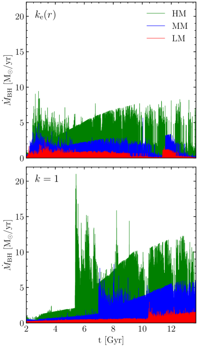
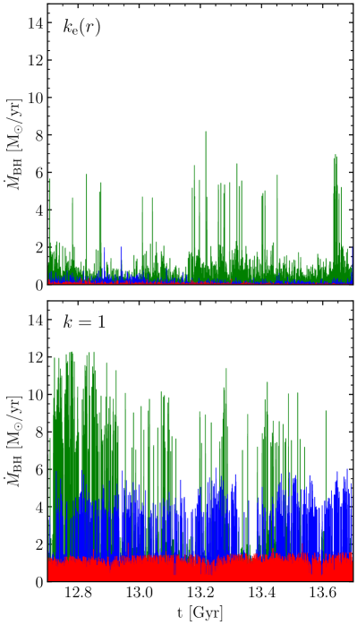
Figure 3.— Time evolution of the SMBHs accretion rate, for the high-mass (green), medium-mass (blue), and low-mass (red) galaxy models, during the whole evolution (left panels), and over the last Gyr (right panels). $\dot{M}_{\rm BH}$ spans a range of $\approx(10^{-5}-10^{-1})\times\dot{M}_{\rm Edd}$, with very few accretion episodes with $\dot{M}_{\rm BH}$ exceeding $\dot{M}_{\rm Edd}$. The different stellar ordered rotation is indicated by the $k$ values in the upper left corner (with $k_{\rm e}(r)$ corresponding to mild rotation, and $k=1$ to isotropic rotators).

¿From inspection of Table 2, we found systematic trends between the mass $\Delta M_{\rm BH}$ accreted by the SMBH at the end of the simulations, and the galaxy mass and the degree of internal ordered rotation.

The first trend is that $\Delta M_{\rm BH}$ increases with galaxy mass. This is not surprsing, as the mass losses from stars scale linearly with the stellar galaxy mass $M_{*}$, and from Equation (18) also the mass accretion from the group/cluster environment scales linearly with the galaxy mass, so that in more massive galaxies more gas is available for accretion. However, from inspection of the $M_{*}$ values in Table 1, one sees that $\Delta M_{\rm BH}$ increases more than linearly with the mass sources, i.e., SMBHs in massive galaxies accrete more efficiently than SMBHs in galaxies of lower mass. This is a quite well established result, a natural byproduct of the larger binding energy per unit mass of more massive galaxies, as dictated by the Faber-Jackson law, which leads to a more efficient gas retention, as the heating sources (thermalization of stellar winds, and SN explosions) scale instead linearly with the galaxy mass (e.g., Ciotti et al. 1991). This is confirmed by the amounts of hot gas retained by the galaxies inside a volume of $5\,\langle R_{\rm e}\rangle$ at the end of the simulations (see Column 9 in Table 2, see also Figure 7).

The second trend is that, in each of the families (LM, MM, and HM), the more rapidly rotating galaxies accrete more material on to their SMBH (see the $\Delta M_{\rm BH}$ evolution in Figure 4, left panels). This result may appear at odds with expectations, as the centrifugal barrier of faster rotating galaxies acts in the sense of preventing accretion (see Figure 2). In fact quite the opposite happens: a stronger rotational favour large scale instabilities and gas cooling over the galaxy body, leading to stronger inflows on the equatorial plane, and to the formation of more massive and extended gaseous disks than in mildy rotating models, where less massive and smaller disks form (see Columns 2 and 3 in Table 2, see also Section 4.2). Toomre instabilities then discharge gas on to the central SMBH, following the prescriptions of Section 3; interestingly, the smaller disks have a higher gas density (Column 4 in Table 2), and are thus more prone to Toomre instability than the more massive and more diffuse gaseous disks of faster rotating models. A check shows that the larger $\Delta M_{\rm BH}$ of fast rotators is due to fewer instability events, characterized though by significantly larger mass accretion episodes.

In Figure 3 we show the time evolution of $\dot{M}_{\rm BH}$ over the whole time interval spanned by the simulations (left panels), and over the last Gyr (right panels). In the top panels the plots refer to the midly rotating models, while in the bottom panels to the isotropic rotators. The dependence of the SMBH accretion rate on galaxy mass and internal rotation is clearly detectable: the accretion episodes reach systematically higher $\dot{M}_{\rm BH}$ in high mass models and in models with substantial internal rotation. The left panels also show how important accretion episodes begin almost immediately in the mildy rotating galaxies (top panel), while the first massive accretion episodes in the isotropic rotators (with peaks of $\dot{M}_{\rm BH}\simeq 10-20\;{\rm M}_{\odot}{\rm yr}^{-1}$) start at quite late times, with the epoch of the first important event increasing at decreasing galaxy mass (bottom panel), with more rotating gas collects at larger radii and lower densities, hence lower lower cooling and later accretion events. At low redshift, peak rates of accretion hardly reach Eddington values, $\dot{M}_{\rm Edd}=L_{\rm Edd}/0.1c^{2}$, with common values of $\dot{M}_{\rm BH}$ in the range $\approx(10^{-5}-10^{-1})\times\dot{M}_{\rm Edd}$.

In the left panels of Figure 4 we plot the function $\Delta M_{\rm BH}=\int\dot{M}_{\rm BH}dt$ as a function of time, where the vertical lines mark the time at which half of the final value of $\Delta M_{\rm BH}$ is reached. The more conspicuous features are the more rapid growth in the mildly rotating models (top panel) than in the isotropic rotators (bottom panel); the jumps of $\Delta M_{\rm BH}$ in the isotropic rotators (corresponding to the jumps in $\dot{M}_{\rm BH}$ in Figure 3, bottom left), absent in the less rapidly rotating galaxies;, and finally the inversion of the time order in which half of the accreted mass is reached, with a faster evolution of the HM model with respect to the LM one, in the isotropic rotator case, while the opposite holds for the $k_{\rm e}(r)$ models. The bottom panels of Figure 4 are consistent with the observed fact that lower mass Seyfert galaxies peak at later epochs than do higher mass Quasars, a dramatic confirmation of our modeling.

Overall, the results in this Section confirm that AGN feedback is efficient to maintain SMBHs masses in the present universe small, when compared to the available gas that could be accreted with unstopped cooling flows (approximately two orders of magnitude more than the final SMBHs masses, even not considering group/cluster accretion). It is also shown how specific properties of ordered rotation can significantly affect the accretion history and the AGN feedback in ETGs. Finally, we notice that the final SMBHs masses obtained in the present simulations are somewhat larger than the observed ones. However, our test models run at higher resolution (with the first radial grid point placed at 2.5 pc from the SMBH, instead of 25 pc as in the model survey here presented) indicate that the final $\Delta M_{\rm BH}$ mass would be appreciably smaller in a still higher resolution simulation, with a significant fraction of the mass that in the quoted simulations falls to the SMBH instead being either ejected or turned into stars. Thus the too large final SMBH masses in the present simulations would probably be reduced to values consistent with the Kormendy and Ho (2013) relation, were we able to proceed to still higher resolution simulations.

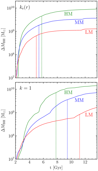
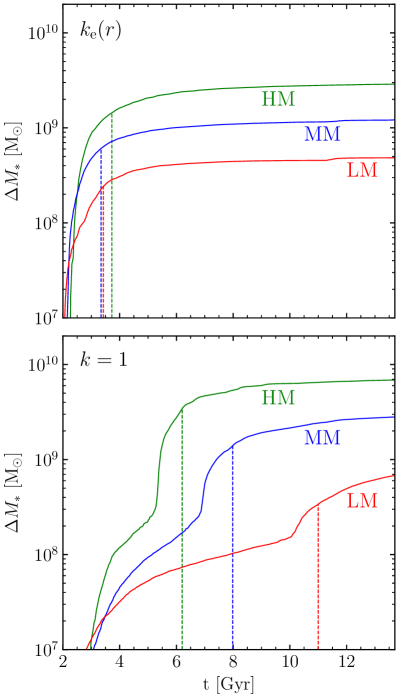
Figure 4.— Left panels: time evolution of the mass $\Delta M_{\rm BH}$ accreted by the central SMBH, for the same models in Figure 3 (high-mass: green, medium-mass: blue, low-mass: red). Right panels: evolution of the time-integrated star formation rate, $\Delta M_{*}$, for the same models in Figure 6; notice that $\Delta M_{*}$ is not the present-day mass of stars formed during the model evolution (cfr. Columns 5 and 7 in Table 2), as a significant fraction of $\Delta M_{*}$ is re-injected in the ISM from mass losses from the newly formed stars. In each plot, the vertical lines mark the time at which each quantity reaches half of its final value. Note haw BH accretion occurs later in lower mass galaxies.

4.2. The equatorial gaseous and stellar disks. Star formation rates

4.2.1 The equatorial disks

With the exception of non rotating models, all models in Table 2 are characterized by different degrees of internal ordered rotation (Section 2.1). It is a natural result of gas cooling in the presence of angular momentum that even in case of low-rotational support of the stellar component, cold gaseous disks form in the equatorial plane of the galaxy. This is because mass injection from the stellar population contributes a source of momentum and angular momentum for the ISM proportional to the local streaming velocity of stars $\overline{v_{\varphi}}$ (e.g., see Equation (53) in G19a, Chapter 10 in Ciotti 2021b). Several works have explored the problem of rotating cooling flows, both numerically with the aid of hydrodynamical simulations (e.g., see Brighenti and Mathews 1996, D’Ercole & Ciotti 1998, Negri et al. 2014a,b, Negri et al. 2015), and analytically (Ciotti & Pellegrini 1996, Posacki et al. 2013). In the above investigations, no AGN feedback was considered. The common findings can be summarized as (1) a substantial and enhanced tendency of the rotating ISM towards instabilitites/cooling (almost absent in non rotating models), (2) a rotational field of the ISM comparable to that of the stars, with the ISM rotational velocity $u_{\varphi}\simeq\overline{v_{\varphi}}$, (3) the formation of cold gaseous disks in the equatorial plane, more or less massive and extended depending on the amount of ordered rotational support, (4) a substantial decrease of the ISM X-ray luminosity $L_{\rm X}$ when compared to that of similar galaxies in absence of rotation. This latter result is interesting, as observations (e.g., see Sarzi et al. 2013, Juranova et al. 2020) seem in fact to indicate that rotating systems tend to be X-ray underluminous when compared with non rotating galaxies of similar optical luminosity.

In the previous studies two major ingredients were missing, namely the effect of disk instabilities/viscosity, and AGN feedback. The two phenomena are clearly related, as in a rotating system the centrifugal barrier would make accretion on the SMBH impossible in the absence viscous effects. We studied in exploratory works the combined effect of rotation and AGN feedback (Ciotti et al. 2017, Pellegrini et al. 2018, Yoon et al. 2018, G19a,b, G20), with a phenomenological description of Toomre instability, angular momentum migration, and mass discharge on the SMBH. In the present study we adopt more realistic galaxy models, an updated treatment of disk instabilites and gas viscosity, and an improved AGN feedback modelization. Overall, for the comprehensive set of rotating models in Table 2 the four main results mentioned above are recovered.

Table 2 lists the final values of the mass $M_{\rm dHI}$ and size $R_{\rm dHI}$ (defined as the truncation radius) of the cold gaseous disks that form in the equatorial plane: they are defined by considering the region with the gas temperature $T\leq T_{\rm c}=5\times 10^{5}$ K. It is apparent how in each of the three families, the final mass of the cold disk $M_{\rm dHI}$ increases with increasing rotational support of the galaxy, and so does the disk size $R_{\rm dHI}$, ranging from a few hundreds pc to a few kpc. The increase of $M_{\rm dHI}$ with rotation, at fixed galaxy structure, testifies to the effect of rotation in enhancing gas cooling over the galaxy body. This can be clearly seen in the left panels of Figure 5, where the time evolution of $M_{\rm dHI}$ is shown. In particular, notice how in the isotropic rotators the epoch of the significant drops of disk mass happens at later times at decreasing galaxy mass, and how the drops coincide with the beginning of strong burst in SMBH accretion (bottom left panels in Figures 3 and 4).

A simple explanation for the increase of $R_{\rm dHI}$ with the importance of galactic rotation, can be obtained by considering the equation for the $z$-component of the angular momentum (per unit mass) $j_{z}$ of the gas flows, subjected to the angular momentum injection due to stellar evolution. Due to the axisymmetry of the simulations, and ignoring for simplicity viscosity effects of the inflows (at variance with the evolution of the cold and dense equatorial disks, where $\alpha$-viscosity is taken into account), it is easy to show that along the pathlines of fluid elements

$${Dj_{z}\over Dt}={\dot{\rho}\over\rho}R\,(\overline{v_{\varphi}}-u_{\varphi}),\quad R=r\sin\theta,$$ (30)

where $D/Dt$ is the usual lagrangian derivative, $\overline{v_{\varphi}}$ is the stellar streaming velocity in Equation (11), $u_{\varphi}$ is the gas azimuthal velocity, and $R$ the cylindrical radius. The numerical simulations show that the velocity difference of gas and stars (in the azimuthal direction) is quite small, so that as a zeroth-order approximation we can assume $j_{z}$ is conserved. This allows us to compute the surfaces of constant $j_{z}=R\,\overline{v_{\varphi}}(R,z)$ (see Figure 2). Under this simplified model, the cooling gas falls onto the equatorial disk at $R_{\rm in}$, where the surfaces of constant $j_{z}$ cross the equatorial plane. However, due to the axysimmetric drift, the rotational velocity of the gas is lower than the galaxy local circular velocity $v_{\rm c}(R)$, and so the gas will move inward, ending on a circular orbit of radius $R_{\rm fin}$, where $R_{\rm in}\overline{v_{\varphi}}(R_{\rm in},0)=R_{\rm fin}v_{\rm c}(R_{\rm fin})$ (see Figure 1, right panel). Figure 2 shows clearly that the gas falls onto the disk at significantly larger radii in the isotropic rotators than in the mildy rotating models. This has interesting consequences: even if the cold gas mass in isotropic rotators is larger than in models of same structure but less rotating, yet the much larger disk size implies a lower gas surface density; as a consequence the more massive disks in isotropic rotators are expected to be less Toomre unstable than the smaller disks in mildly rotating galaxies of same structure. These expectations are confirmed by the time evolution of the mean gas surface density, defined as $\langle\Sigma_{\rm dHI}\rangle=M_{\rm dHI}/(\pi R_{\rm dHI}^{2})$, shown in the right panels of Figure 5, and Table 2. We conclude that the larger final masses of the SMBH in isotropic rotators is a consequence not of more instability events, but of fewer instabilities each involving larger amounts of mass, due to the larger $M_{\rm dHI}$.

Quite naturally, the above findings are also found in the evolution of star formation, as disk instabilities are related both to SMBH accretion and star formation.

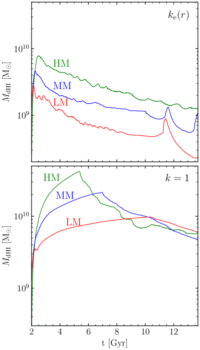
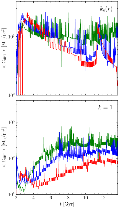
Figure 5.— Left panels: time evolution of the total mass of cold gas present in the equatorial disk, for the high-mass (green), medium-mass (blue), and low-mass (red) galaxy models, over the whole cosmic time spanned by the simulations. The different amounts of ordered stellar rotation are indicated by $k=k_{\rm e}(r)$ (mild rotation), and by $k=1$ (isotropic rotators). Right panels: time evolution of the average gas surface density of the disks, defined as $M_{\rm dHI}/(\pi R_{\rm dHI}^{2})$, for the same models in the left panels.

4.2.2 Star formation

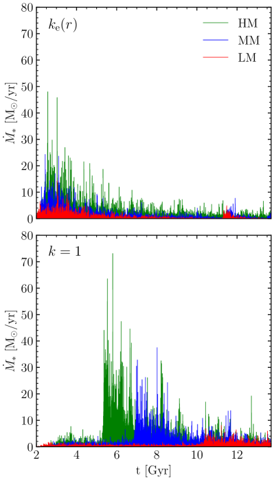
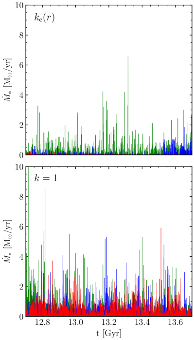
Figure 6.— Time evolution of the star formation rate, for the high-mass (green), medium-mass (blue), and low-mass (red) galaxy models, over the whole simulated time (left panels), and over the last Gyr (right panels). The different amount of galactic rotation in the galaxy stellar population is indicated by $k=k_{\rm e}(r)$ (mild rotation), and by $k=1$ (isotropic rotators).

As anticipated in Section 3, Toomre instabilities in the equatorial gaseous disk not only lead to mass accretion events on the SMBH, but also produce local bursts of star formation, as apparent by comparing Figures 3 and 6, where the SMBH accretion rates ($\dot{M}_{\rm BH}$) and the star formation rates ($\dot{M}_{*}$) are shown as a function of time. The parallel evolution of SMBH accretion (and AGN activity) and star formation is also visibile in Figure 4, where in the right panels we show the cumulative star formation $\Delta M_{*}$ in the galaxy. Again, in the isotropic rotator case, the less massive galaxies evolve with longer time scales than more massive systems, as can be seen from the position of the vertical lines in the bottom-right panel, marking the epoch when half of the total star formation in each galaxy has been reached.

In the simulations, we assume for simplicity that the newly formed stars stay on the circular orbit where they form, and we then follow their evolution, that contributes mass losses, and SNII explosions. At the end of the simulations, stellar disks of mass $M_{\rm d*}\simeq 10^{8}-10^{9}{\rm M}_{\odot}$, and half-mass radius $R_{\rm d*}\simeq 100-300$ pc, are present in the equatorial plane (Columns 5 and 6 in Table 2); notice that in each family of models the trend of $M_{\rm d*}$ and $R_{\rm d*}$ with the galaxy mass and rotational support nicely follows the trends of the gaseous disks parameters ($M_{\rm dHI}$ and $R_{\rm dHI}$). The stellar disks are significantly more concentrated ($R_{\rm d*}<R_{\rm dHI}$) as a consequence of the density dependence of the star formation algorithm. Of course, from the stellar formation prescription in G19a, star formation is not necessarily limited to the equatorial gaseous disk; but in the simulations almost all the star formation takes place in the disk: the difference between $\Delta M_{*}$ and $M_{\rm d*}$ is fully explained by the star evolution and mass losses in the (top-heavy) secondary star generations. The inevitable formation of second-generation, metal rich ($\alpha$-enhanced) stellar disks produced by the gas recycled by stars in the galaxy, is an important prediction of the present models, that will be discussed in depth in a dedicated paper; notice that these stellar disks are always corotating with the parent galaxy, because the intrisic mechanism cannot produce counterrotating disks, and the material from the circumgalactic medium is assumed to be accreted on radial orbits.

4.3. X-ray luminosities and temperatures of the hot ISM coronae

The last group of quantities characterizing the evolutionary properties of the hot ISM, are the final values of the total amount of hot gas $M_{\rm hot}$ ($T>T_{\rm c}=5\times 10^{5}$ K), the X-ray luminosity in the usual $0.3-8$ keV energy band, and measured inside the obervational aperture of $r_{\rm X}=5\langle R_{\rm e}\rangle$, and finally the emission-weighted temperature $T_{\rm X}$ measured inside the same aperture (see Table 2). An additional quantity useful to check the mass conservation of the code is the amount of gas $M_{\rm out}$ lost at the last radial grid point ($250$ kpc); in fact for each run we monitored the mass balance over the whole numerical grid due to the mass sources and sinks, obtaining an execellent agreement (notice that $M_{\rm out}$ and $M_{\rm hot}$ reported in Table 2 cannot be directly compared, being measured over different volumes).

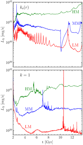
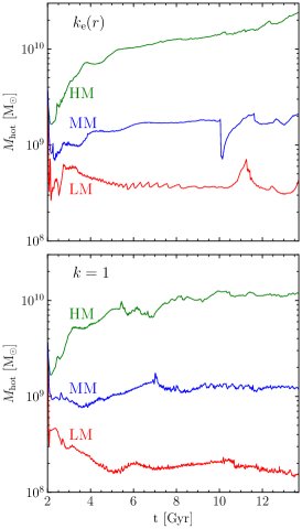
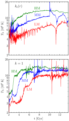
Figure 7.— Left panels: time evolution of the X-ray luminosity $L_{\rm X}$ of the ISM measured in the energy band of $0.3-8$ keV, inside a sphere of radius $r_{\rm X}=5\,\langle R_{\rm e}\rangle$ (see Table 1), and excluding the inner 100 pc to reduce the fluctuations due to AGN activity. Green, blu, and red lines refer to HM, MM, and LM models, respectively; note how more ordered galaxy rotation (bottom panel) reduces $L_{\rm X}$, at fixed galaxy structure. Central panels: time evolution of the mass $M_{\rm hot}$ of the hot ISM ($T>T_{\rm c}=5\times 10^{5}$ K) contained within a sphere of radius $r_{\rm X}=5\langle R_{\rm e}\rangle$. A close parallel between $L_{\rm X}$ and $M_{\rm hot}$ is apparent, with a substantial reduction of $M_{\rm hot}$ in the isotropic rotators. Right panels: the emission-weighted X-ray temperature of the ISM, over the same volume used for the computation of $L_{\rm X}$.

In Figure 7 we show the time evolution of $M_{\rm hot}$, $L_{\rm X}$, and $T_{\rm X}$; reassuringly, the values of $L_{\rm X}$ and $T_{\rm X}$ agree with those observed: the final $L_{\rm X}$ and $T_{\rm X}$ in Table 2 exhibit a range of values that compares very well with that reported for the large number of ETGs in the $Chandra$ Galaxy Atlas (Kim et al. 2019), and in the $Chandra$ sample of Kim and Fabbiano (2015), for galaxies of comparable mass. Also, the range of $L_{\rm X}$ shown by the models both covers most of the observed range, and progressively moves to larger values with increasing galaxy mass, as observed. A few trends are clearly detectable: first, $L_{\rm X}$ and $T_{\rm X}$ in each family of models correlate with the total mass of the galaxy, being more massive galaxies more X-ray luminous and hotter than less massive systems, a well know manifestation of the underlying Faber-Jackson relation. Second, $T_{\rm X}$ tends to increase with time, while $L_{\rm X}$ can span a range up to two orders of magnitude (for a range of 5 in the stellar masses in the explored models). Third, for fixed galaxy mass, less rapidly rotating systems are more X-ray luminous than their isotropic rotator counterparts. Thus, we confirm that, at each mass, rotation tends to reduce the X-ray luminosity of ETGs, due to the tendency of rotating flows to induce gas cooling at relatively large radii (e.g., Negri et al. 2014a,b; Gaspari et al. 2015). This finding is in accordance with X-ray observations that show flatter systems (that are typically more rapidly rotating objects) to have a lower $L_{\rm X}$ than rounder ones of the same optical luminosity (Eskridge et al. 1995; Sarzi et al. 2013; see also Juranova et al. 2020). In particular, Sarzi et al., using data from the ATLAS^3D survey, found fast rotators to have lower $L_{\rm X}$ and $T_{\rm X}$ than slow rotators. The simulations also predict extended hot gas cooling, in rotating systems, and then a larger tendency for them to host (large) cold disks. Indeed, gas forming disks in the equatorial plane of ETGs (and aligned with the rotation of the stars) has been detected from the ionized to the atomic (HI) to the molecular (CO) phase, and preferentially in fast rotators (Young et al. 2011, Davis et al. 2019, Juranova et al. 2019; see also Babyk et al. 2019). Finally, a paper is in preparation, specifically dedicated to a thorough analysis of the X-ray properties of the models, including the radial profiles of their X-ray surface brightness, and of their luminosity-weighted projected temperature, to be compared with those typically observed.

Also note the solution to the classical “cooling flow problem” indicated by our numerical solutions. While some (metal enriched) gas falls to the center, as revealed by $\Delta M_{\rm BH}$, $M_{\rm dHI}$, and $M_{\rm d*}$, $\approx 30$ times more gas ($M_{\rm out}$) is expelled by feedback, as reported in Column 9 of Table 2. In general, rotating models (with the exception of HM family) tend to eject more mass as the rotational support of the galaxy increases, because rotation not only increases the tendency for gas cooling, but also unbinds gas at large radii (see e.g. Cotti and Pellegrini 1996, Posacki et al. 2014, Negri et al. 2014b); thus the net effect of substantial rotation is to produce more cold gas and less hot ISM, leading to an X-ray underluminosity and lower hot gas temperatures.

5. Discussion and conclusions

In this paper we presented a first, systematic exploration of the hot gas evolution for a set of realistic high resolution models of massive ETGs with central SMBHs. The exploration was conducted with the latest version of the high-resolution 2D hydrodynamical code MACER. The innermost grid point was placed at 25 pc from the center, the outermost at 250 kpc, and the flow evolution was followed at high temporal resolution over the cosmological time span of 12 Gyr. A few, time-expensive test simulations, were also conducted with a much higher spatial resolution, with the first active grid point placed at 2.5 pc from the SMBH. The initial stellar mass of the galaxy models is in the range $1.5\times 10^{11}<M_{*}/{\rm M}_{\odot}<7.8\times 10^{11}$, and has the E3 shapes when observed edge-on. The stellar density distribution, and the DM halo associated with the galaxies, are modeled by two-component ellipsoidal Jaffe profiles (JJe models, CMPZ21), providing a very good approximation over a large radial range of the de Vaucouleurs and the NFW profiles, respectively; a group/cluster quasi-isothermal DM halo with a flat rotation curve in the outer regions is also considered. The internal dynamics of the galaxies is obtained by solving the Jeans equations, and for each model we explore the non-rotating case (when the galaxy flattening is fully supported by tangential velocity dispersion), the isotropic rotator (when galaxy flattening is fully supported by ordered rotation), and an intermediate case with exponentially declining ordered rotation, obtained from a spatially dependent Satoh decomposition. Mass sources are represented by mass losses from stars (red giants, AGB stars, and SNIa/SNII explosions, computed following the prescriptions of stellar evolution), and by a time-dependent cosmologically motivated mass accretion rate from the group/cluster ambient, imposed at the outer boundary of the numerical grid. In rotating models the stellar mass losses are injected in the ISM following the galaxy ordered velocity field, and the cooling gas collapses on to a rotating gaseous disk in the equatorial plane. Tqhe ISM is heated by thermalization of the kinetic energy of SNe explosions, and stellar motions; gas cooling is implemented as in our previous version of MACER (G19a); the production and circulation of metals, and the formation/destruction of dust, are also considered following G20. Two different channels are considered for star formation: the classical one based on the cooling and and the Jeans collapse times of the ISM, and a second based on the assumption that the rotating gaseous disk self-regulates due to Toomre instabilities around a value of $Q\simeq 1$. These instabilites lead to bursts of star formation, the formation of a central rotating stellar disk, outward angular momentum transport and inward mass transport (in addition to the effects of standard $\alpha$-viscosity, also considered in the simulations), and finally to SMBH accretion and AGN feedback.

As a first improvement over our previous simulations, we consider the secular evolution of the galaxy gravitational field due to mass losses of stars (in addition to the changes of the gravitational field due to the mass growth of the SMBH, already considered in our previous studies); we also implemented the associated changes of the velocity dispersion and rotational fields of the stars. In rotating models, the effects of the time-evolving gravitational field of the equatorial stellar disk on the gas flows, are also taken into account. As a second important improvement we now model the UV heating effects of the massive, young stars in the stellar disk, in addition to the disk SNII feedback. The third set of improvements concerns the treatment of AGN feedback. In particular we adopt a higher maximum wind efficiency $\epsilon_{\rm w}^{\rm M}$ in the cold-accretion mode, and a smoother transition of $\epsilon_{\rm w}$ between cold and hot accretion regimes.

The main results can be summarized as follows. In general, we confirm the picture that the evolution of the ISM undergoes recurrent cycles, during which the gas cools, falls towards the central galactic regions, and – if it possesses angular momentum – accumulates in a central disk; there, it becomes over-dense and self-gravitating, until in the disk the Toomre instability sets in, allowing for star formation and mass inflow from the disk towards the SMBH. The errupting SMBH then ejects much of the inflowing material back into the ISM. Thus, with a short delay (of the order of the orbital period of the circumnuclear disk), star formation is followed by accretion of disk material onto the SMBH. An AGN burst is then triggered, and the energy output from the galactic centre, in the form of radiation and winds, modifies the hydrodynamics of the ISM throughout the host galaxy (which is known as the AGN feedback). The biconical AGN winds cause the ejection of gas into the polar regions, but also the other galactic regions are affected more or less directly by the propagation of shock waves, with the consequent alternate compression and rarefaction. After a starburst, the massive stars can also feed energy back to the ISM via SNII explosions; this impacts mostly the region around where star formation occurs (over a lengthscale of $\sim 1$ kpc). Most of the SNII events occur within the cold rotating (and dusty) disk, but in some models we allow for 40% of the SNII to arise from runaway stars which have typically travelled 100–300 pc away from their birthplaces. The new stars in the central disk form with a top heavy mass function as found in the MW and M31 (see also Goodman and Tan 2004). They are embedded in a dusty cool gas envelope which will have notable IR emission properties (see e.g. G19b), in agreement with observations.

More in detail, we focused on three specific properties of the model evolution, considering both the effects of the galaxy mass, and of the degree of internal rotation.

For what concerns SMBH accretion, we found (not suprisingly) that $\Delta M_{\rm BH}$ increases with galaxy mass, but more than linearly with the mass sources, i.e., SMBHs in massive galaxies accrete more efficiently than SMBHs in galaxies of lower mass, a natural consequence of the scaling with galaxy mass of heating sources and the depth of the galaxy potential well, with the SMBH mass accretion (and AGN feedback) peaking earlier in the high mass systems. Moreover, at fixed galaxy mass the more rapidly rotating galaxies accrete more material on to their central SMBH. This is due to the fact that a stronger rotation tends to favour large scale instabilities and gas cooling, leading to stronger inflows, and the formation of more massive and extended gaseous disks. The larger $\Delta M_{\rm BH}$ of fast rotators is due to fewer instability events in the disk, characterized though by significantly larger mass accretion. In fact, accretion reaches systematically higher $\dot{M}_{\rm BH}$ in high mass models and in models with substantial internal rotation. Important accretion episodes begin almost immediately in the mildy rotating galaxies, while the first massive accretion episodes in the isotropic rotators start at quite late times, with the epoch of the first important event increasing at decreasing galaxy mass. It is intriguing to speculate that these trends may help to explain the empirical observation that the activity of lower mass Seyfert galaxies peaks at later epochs than do higher mass Quasars. Overall, the results in this Section confirm that AGN feedback is efficient to maintain SMBHs masses in the present universe small, when compared to the available gas that could be accreted with unstopped cooling flows.

For what concerns the formation of the equatorial gaseous disk, its instabilites, and the associated star formation, we confirmed that gas cooling, even in presence of moderate rotational support of the stellar component, produces cold gaseous disks in the equatorial plane, with present day masses in the range $10^{8}{\rm M}_{\odot}-10^{9}{\rm M}_{\odot}$, sizes ranging from a fraction of kpc to a few kpc, and surface densities of $\approx 10^{2}{\rm M}_{\odot}/{\rm pc}^{2}$; masses and disk sizes increase for increasing galaxy mass and amount of rotational support. Interestingly, even if the mass of the cold disks in isotropic rotators is larger than in models of same structure but less rapidly rotating (due to the well known enancement of cooling efficiency in rotating models), yet the much larger size implies a lower gas surface density, so that the more massive disks in isotropic rotators are in general less Toomre unstable than the smaller disks in moderatly rotating galaxies of same structure. An interesting consequence of this behavior is that the larger final masses of the SMBH in isotropic rotators are a consequence not of more instability events, but of fewer instabilities each involving larger amounts of mass, due to the larger values of $M_{\rm dHI}$. As instabilities in the gaseous disk, not only lead to mass accretion events on the central SMBH, but also produce local bursts of star formation, we also found at the end of the simulations, stellar disks of mass $M_{\rm d*}\simeq 10^{8}{\rm M}_{\odot}-10^{9}{\rm M}_{\odot}$, and half-mass radii $R_{\rm d*}\simeq 100{\rm pc}-300$ pc, in the galaxy equatorial plane; in each family of models the dependence of $M_{\rm d*}$ and $R_{\rm d*}$ on the amount of galaxy mass and rotational support nicely follows the trends of the gaseous disks properties $M_{\rm dHI}$ and $R_{\rm dHI}$. Moreover, in the isotropic rotator case, the less massive galaxies evolve with longer time scales than the more massive systems.

Finally, for what concerns the X-ray properties of the hot gas, in our systematic exploration of parameter space, the values of $L_{\rm X}$ (the X-ray luminosity inside $5\langle R_{\rm e}\rangle$ and in the energy band of 0.3-8 keV) and of $T_{\rm X}$ (the associated emission-weighted temperature over the same volume) are in the observed range, with more massive galaxies hosting more luminous gaseous halos. In each mass range, the isotropic rotators are found at a lower luminosity than models of similar structure but less rapidly rotating, confirming that rotation tends to reduce the X-ray luminosity of galaxies, due to the strong tendency of rotating flows to induce gas cooling. We also confirm the strong sensitivity of X-ray luminosity on the galaxy mass, with $L_{\rm X}$ spanning a range up to two orders of magnitude, for a range of a factor of 5 in the stellar masses.

There are numerous observational checks possible to determine if we have adequately modelled the evolution of gaseous halos of massive galaxies, and we list here some of them. Do the final hot X-ray properties agree with observations in terms not only of intergrated properties, but also on detailed radial profiles of $\Sigma_{\rm X}$ and $T_{\rm X}$? Does the amount and metallicity of the expelled gas correspond to the observed CGM? Do the predicted circumnuclear gas and stellar disks exist in the real world? Of course mergers, which we neglect, would tend to disrupt and disperse this component. Do the outflowing winds seen in AGN have the high metal content – in particular the $\alpha$-enhanced abundances – predicted by our models as a consequence of top-heavy star formation in the central disk? What is the effect of a nuclear jet on the galaxy evolution? What new phenomena are associated with genuine 3D hydrodynamics? Further papers in this series will address some of these questions.

Appendix A Stellar velocity dispersions

The solution of the Jeans equations for the galaxy stellar component (excluding for simplicity the contribution of the group/cluster quasi-isothermal DM halo and of the time-dependent equatorial stellar disks, see Section 2.1) can be written as

$$\sigma_{*}^{2}=\sigma_{*{\rm BH}}^{2}+\sigma_{*{\rm g}}^{2},\qquad\Delta_{*}=\Delta_{*{\rm BH}}+\Delta_{*{\rm g}},$$ (A1)

where $\sigma_{*{\rm BH}}$ and $\sigma_{*{\rm g}}$ represent the contribution of the central SMBH and of the galaxy potential to the radial and vertical components of the velocity dispersion tensor, and similarly for the quantity $\Delta_{*}=\overline{v_{\varphi}}^{2}+\sigma_{\varphi}^{2}-\sigma_{*}^{2}$. For the considered models, in the special case of a spherically symmetric total (stars plus DM) density distribution, the general solutions (see CMPZ21) reduce to

$$\rho_{*}\sigma_{*{\rm BH}}^{2}={GM_{*}^{2}\mu\over 4\pi r_{*}^{4}}\left[A(s)+\eta_{*}B(s)+\eta_{*}C(s)s^{2}\sin^{2}\theta\right],\quad\rho_{*}\Delta_{*{\rm BH}}={GM_{*}^{2}\mu\over 2\pi r_{*}^{4}}\eta_{*}C(s)s^{2}\sin^{2}\theta,$$ (A2)

$$\rho_{*}\sigma_{*{\rm g}}^{2}={GM_{*}^{2}{\cal R}\over 4\pi r_{*}^{4}}\left[D(s,\xi)+\eta_{*}E(s,\xi)+\eta_{*}F(s,\xi)s^{2}\sin^{2}\theta\right],\qquad\rho_{*}\Delta_{*{\rm g}}={GM_{*}^{2}{\cal R}\over 2\pi r_{*}^{4}}\eta_{*}F(s,\xi)s^{2}\sin^{2}\theta,$$ (A3)

where $s=r/r_{*}$ and

$$A(s)={12s^{3}+6s^{2}-2s+1\over 3s^{3}(1+s)}+4\ln{s\over 1+s},\quad B(s)={24s^{4}+36s^{3}+8s^{2}-2s-1\over 3s^{3}(1+s)^{2}}+8\ln{s\over 1+s},$$ (A4)

$$C(s)=-{180s^{6}+270s^{5}+60s^{4}-15s^{3}+6s^{2}-3s-4\over 10s^{5}(1+s)^{2}}-18\ln{s\over 1+s}.$$ (A5)

$$D(s,\xi)=-{3\xi^{2}-\xi-1\over\xi^{2}(\xi-1)(1+s)}-{(3\xi+2)s-\xi\over 2\xi^{2}s^{2}(1+s)}-{1\over\xi^{3}(\xi-1)^{2}}\ln{s\over\xi+s}-{3\xi-4\over(\xi-1)^{2}}\ln{s\over 1+s},$$ (A6)

$$E(s,\xi) = -\frac{2(3\xi^{3}-6\xi^{2}+2\xi-1)s+9\xi^{3}-18\xi^{2}+9\xi-4}{2\xi^{2}(\xi-1)^{2}(1+s)^{2}}-\frac{2(\xi-1)s+\xi}{2\xi^{2}s^{2}(1+s)^{2}}$$ (A7)

$$+ \,\frac{3\xi-1}{\xi^{3}(\xi-1)^{3}}\ln\frac{s}{\xi+s}-\frac{3\xi^{2}-9\xi+8}{(\xi-1)^{3}}\ln\frac{s}{1+s},$$ (A8)

$$F(s,\xi) = \frac{2(5\xi^{5}-8\xi^{4}+\xi^{3}+\xi^{2}+\xi-1)s+15\xi^{5}-24\xi^{4}+3\xi^{3}+3\xi^{2}+5\xi-4}{\xi^{4}(\xi-1)^{2}(1+s)^{2}}$$ (A9)

$$+ \,\frac{4(5\xi^{3}+2\xi^{2}-3)s^{3}-\xi(5\xi^{2}+2\xi-6)s^{2}+2\xi^{2}(\xi-2)s+3\xi^{3}}{6\xi^{4}s^{4}(1+s)^{2}}$$ (A10)

$$- \frac{2(2\xi-1)}{\xi^{5}(\xi-1)^{3}}\ln\frac{s}{\xi+s}+\frac{2(5\xi^{2}-13\xi+9)}{(\xi-1)^{3}}\ln\frac{s}{1+s}.$$ (A11)

Finally, the functions $D$, $E$, and $F$ need a separate treatment for the special case $\xi=1$, when

$$D(s,1)=-{(6s^{2}+6s-1)(2s+1)\over 2s^{2}(1+s)^{2}}-6\ln{s\over 1+s},\quad E(s,1)=-{12s^{4}+30s^{3}+22s^{2}+3s+3\over 6s^{2}(1+s)^{3}}-2\ln{s\over 1+s},$$ (A12)

$$F(s,1)={60s^{6}+150s^{5}+110s^{4}+15s^{3}-3s^{2}+s+3\over 6s^{4}(1+s)^{3}}+10\ln{s\over 1+s}.$$ (A13)

Appendix B Gravitational effects of stellar mass losses and SMBH growth

One of the useful features of the adopted analytical models for galaxies is the possibility to easily implement in the hydrodynamical code the secular changes of the gravitational field of the galaxy and of the stellar velocity dispersion and rotational fields of the stars due to the mass growth of the central SMBH and to the reduction of the stellar mass due to the stellar mass losses. Moreover, as described in Sections 2.1 and 3, we also consider the effects of the time independent gravitational field of a group/cluster DM halo, and the time dependent gravitational field of the stellar equatorial disk produced by the rotating cooling gas: hower, for simplicity we neglect the effects of these two gravitational fields on the velocity fields of stars.

The stellar mass losses (stellar winds plus SNIa explosions) produce a mass source term $\dot{\rho}=\alpha(t)\rho_{*}$ in the hydrodynamical equations, where the function $\alpha(t)$ is prescribed by stellar evolution (see e.g. Pellegrini 2012; Ciotti & Ostriker 2012 for details). We define the mass reduction factor

$$f(t)=1-\epsilon(t),\qquad\epsilon(t)\equiv\int_{2{\rm Gyr}}^{t}\alpha(\tau)d\tau,$$ (B1)

so that

$$M_{*}(t)=f(t)M_{*},\quad\rho_{*}(t)=f(t)\rho_{*},\quad\phi_{*}(t)=f(t)\phi_{*},$$ (B2)

and in the following all quantities independent of time refer to the initial time of the simulations (when as usual the stellar population is assumed to be 2 Gyr old). In particular, in equation above $\phi_{*}$ is the potential at the beginning of the simulations of the ellipsoidal Jaffe stellar distribution in Equation (3), obtained for simplicity by homeoidal expansion

$$\phi_{*}={GM_{*}\over r_{*}}\left[\tilde{\phi}_{*0}(s)+\eta_{*}\tilde{\phi}_{*1}(s)+\eta_{*}\tilde{\phi}_{*2}(s)s^{2}\sin^{2}\theta\right],\quad\tilde{\phi}_{*i}=\begin{cases}\displaystyle{\ln{s\over 1+s}},\qquad(i=0),\\ \displaystyle{{s^{2}+2s+4\over 3s^{2}(1+s)}+{1\over 3}\ln{s\over 1+s}-{4\ln(1+s)\over 3s^{3}}},\quad(i=1),\\ \displaystyle{-{s+2\over s^{4}(1+s)}+{2\ln(1+s)\over s^{5}}},\quad(i=2),\end{cases}$$ (B3)

(see Equation 19 in CMPZ21, with $\xi={\cal R}=1$ and $\eta_{\rm g}=\eta_{*}$ therein). Notice that in terms of the initial quantities,

$${\cal R}(t)\equiv{M_{\rm g}(t)\over M_{*}(t)}={{\cal R}-\epsilon(t)\over f(t)},\quad\mu(t)\equiv{M_{\rm BH}(t)\over M_{*}(t)}={\mu\over f(t)}{M_{\rm BH}(t)\over M_{\rm BH}}.$$ (B4)

The total gravitational potential experienced by the gas flows can be written

$$\phi_{\rm tot}(t)=\phi_{\rm g}+\phi_{\rm h}+{M_{\rm BH}(t)\over M_{\rm BH}}\phi_{\rm BH}+\phi_{\rm d*}(t)-\epsilon(t)\phi_{*},$$ (B5)

where $\phi_{\rm g}$, $\phi_{\rm h}$, $\phi_{\rm BH}$ and $\phi_{\rm d*}(t)$ are given respectively by Equations (4), (7), (10) and (25).

Finally, we obtain the expression for the time dependence of the vertical (and radial) velocity dispersion $\sigma_{*}$ and of the function $\Delta_{*}$ needed in Equation (11) to determine the azimuthal velocity dispersion and the streaming velocity of stars. From the dependence of the Jeans equations on the total potential, and from the considerations above, it is easy to show that

$$\sigma_{*}^{2}(t)=\sigma_{*{\rm g}}^{2}+{M_{\rm BH}(t)\over M_{\rm BH}}\,\sigma_{*{\rm BH}}^{2}-\epsilon(t)\sigma_{**}^{2},\quad\Delta_{*}(t)=\Delta_{*{\rm g}}+{M_{\rm BH}(t)\over M_{\rm BH}}\,\Delta_{*{\rm BH}}-\epsilon(t)\Delta_{**},$$ (B6)

where the time independent quantities $\sigma_{*{\rm g}}$, $\Delta_{*{\rm g}}$, $\sigma_{*{\rm BH}}$ and $\Delta_{*{\rm BH}}$ are obtained from Equations (A1)-(A2) by using Equation (1). $\sigma_{**}$ and $\Delta_{**}$ describe the self-contribution of the stellar distribution. From Equations (39) and (41) in CMPZ21 one obtains

$$\rho_{*}\sigma_{**}^{2}={GM_{*}^{2}\over 4\pi r_{*}^{4}}\left[D(s,1)+\eta_{*}X(s)+\eta_{*}Y(s)s^{2}\sin^{2}\theta\right],\quad\rho_{*}\Delta_{**}={GM_{*}^{2}\over 2\pi r_{*}^{4}}\eta_{*}Z(s)s^{2}\sin^{2}\theta,$$ (B7)

where

$$X(s) = {86s^{6}+185s^{5}+101s^{4}-s^{3}-4s^{2}-4\over 5s^{4}(1+s)^{3}}-{34\over 5}\ln{s\over 1+s}$$ (B8)

$$+ 2\left[{60s^{5}+30s^{4}-10s^{3}+5s^{2}-3s+2\over 5s^{5}(1+s)}+12\ln{s\over 1+s}\right]\ln(1+s)-24{\cal H}(1,s),$$ (B9)

$$Y(s) = -{4572s^{8}+10170s^{7}+6002s^{6}+198s^{5}-90s^{4}+44s^{3}-60s^{2}-15s-90\over 63s^{6}(1+s)^{3}}+{52\over 7}\ln{s\over 1+s}$$ (B10)

$$- 2\left[{840s^{7}+420s^{6}-140s^{5}+70s^{4}-42s^{3}+28s^{2}-20s+15\over 21s^{7}(1+s)}+40\ln{s\over 1+s}\right]\ln(1+s)+80{\cal H}(1,s),$$ (B11)

$$Z(s) = -2{2286s^{7}+2799s^{6}+202s^{5}-103s^{4}+58s^{3}-36s^{2}+6s+18\over 63s^{6}(1+s)^{2}}+{52\over 7}\ln{s\over 1+s}$$ (B12)

$$- 2\left[{840s^{8}+1260s^{7}+280s^{6}-70s^{5}+28s^{4}-14s^{3}+8s^{2}-5s-6\over 21s^{7}(1+s)^{2}}+40\ln{s\over 1+s}\right]\ln(1+s)+80{\cal H}(1,s).$$ (B13)

and the function ${\cal H}(\xi,s)$ is defined in Equation (83) of CMPZ21.

References

- Auger (2010) Auger, M. W., Treu, T., Bolton, A. S., Gavazzi, R., Koopmans, L. V. E., Marshall, P. J., Moustakas, L. A., Burles, S. 2010, ApJ, 724, 511
- Babyk (2018) Babyk, Iu. V., McNamara, B. R., Nulsen, P. E. J., Hogan, M. T., Vantyghem, A. N., Russell, H. R., Pulido, F. A., Edge, A. C. 2018, ApJ, 857, 32
- Barnabè (2011) Barnabè, M., Czoske, O., Koopmans, L. V. E., Treu, T., Bolton, A.S. 2011, MNRAS, 415, 2215
- Bellstedt (2018) Bellstedt, S. 2018, MNRAS, 476, 4543
- Bertin (1999) Bertin, G., Lodato, G. 1999, A&A, 350, 694
- Binney (2008) Binney, J., Tremaine, S. 2008, Galactic Dynamics, 2nd ed. Princeton University Press, Princeton, NJ
- Brighenti (1996) Brighenti, F., Mathews, W. G. 1996, 470, 747
- Brighenti (1997) Brighenti, F., Mathews, W. G. 1997, 490, 592
- Caravita (2021) Caravita, C., Ciotti, L., Pellegrini, S. 2021, MNRAS, 506, 1480
- Cappellari (2015) Cappellari, M., Romanowsky, A.J., Brodie, J.P., Forbes, D.A., Strader, J., Foster, C., Kartha, S.S., Pastorello, N., Pota, V., Spitler, L.R., Usher, C., Arnold, J.A. 2015, ApJL, 804, L21
- Ciotti (2001) Ciotti, L., Ostriker, J. P. 2001, ApJ, 551, 131
- Ciotti (2007) Ciotti, L., Ostriker, J. P. 2007, ApJ, 665, 1038
- Ciotti (2011) Ciotti, L., Ostriker, J. P. 2011, ApJ, 737, 26
- Ciotti (2012) Ciotti, L., & Ostriker, J. P. 2012, in Hot Interstellar Matter in Elliptical Galaxies, Vol. 378, ed. D.-W. Kim & S. Pellegrini (New York: Springer), 83
- Ciotti (1996) Ciotti, L., Pellegrini, S. 1996, MNRAS, 279, 240
- Ciotti (2017) Ciotti, L., Pellegrini, S., Negri, A., Ostriker, J.P. 2017, ApJ, 835, 15
- Ciotti (2019) Ciotti, L., Mancino, A., Pellegrini, S. 2019, MNRAS, 490, 2656
- Ciotti (2021a) Ciotti, L., Ziaee Lorzad, A. 2018, MNRAS, 473, 5476
- Ciotti (2021a) Ciotti, L., Mancino, A., Pellegrini, S., Ziaee Lorzad, A. 2021a, MNRAS, 500, 1054 (CMPZ21)
- Ciotti (2021b) Ciotti, L. 2021b, Introduction to Stellar Dynamics, Cambridge University Press, Cambridge, UK
- Cossins (2009) Cossins, P., Lodato, G., Clarke, C.J. 2009, MNRAS, 393, 1157
- D’Ercole (1998) D’Ercole, A., Ciotti, L. 1998, ApJ, 494, 535
- Draine (2011) Draine, B.T. 2011, ”Physics of the Interstellar and Intergalactic Medium”, Princeton University Press (Princeton)
- Eskridge (1995) Eskridge, P.B., Fabbiano, G., Kim, D.-W. 1995, ApJS, 97, 141
- Gan (2019a) Gan, Z., Ciotti, L., Ostriker, J.P., Yuan, F. 2019a, ApJ, 872, 167 (G19a)
- Gan (2019b) Gan, Z., Choi, E., Ostriker, J.P., Ciotti, L., Pellegrini, S. 2019b, ApJ, 875, 109 (G19b)
- Gan (2020) Gan, Z., Hensley, B. S., Ostriker, J. P., Ciotti, L., Schiminovich, D., Pellegrini, S. 2020, ApJ, 901, 7 (G20)
- Gavazzi (2007) Gavazzi, R., Treu, T., Rhodes, J.D., Koopmans, L. V. E., Bolton, A.S., Burles, S., Massey, R.J., Moustakas, L.A. 2007, ApJL, 667, 176
- Goodman (2004) Goodman, J., Tan, J.C. 2004, ApJ, 608, 108
- Juranova (2020) Juranova, A., Werner, N. Nulsen, P. E. J., Gaspari, M., Lakhchaura, K., Canning, R. E. A., Donahue, M., Hroch, F., Voit, G. M. 2020, MNRAS, 499, 5163
- Kim (2012) Kim, D.-W., Pellegrini, S. 2012, ”Hot Interstellar Matter in Elliptical Galaxies”, Astrophysics and Space Science Library, vol. 378, Springer
- Kim (2015) Kim, D.-W., Fabbiano, G. 2015, ApJ, 812, 127
- Kim (2019) Kim, D.-W., Craig, A., Douglas, B., D’Abrusco, R., Fabbiano, G., Fruscione, A., Lauer, J., McCollough, M., Morgan, D., Mossman, A., O’Sullivan, E., Paggi, A., Vrtilek, S., Trinchieri, G. 2019, ApJS, 241, 36
- Koopmans (2009) Koopmans, L. V. E., Bolton, A., Treu, T., Czoske, O., Auger, M. W., Barnabè, M., Vegetti, S., Gavazzi, R., Moustakas, L. A., Burles, S. 2009, ApJL, 703, L51
- Kormendy (2013) Kormendy, J., Ho, L. C. 2013, ARAA, 51, 511
- Li (2018) Li, R., Shu, Y., Wang, J. 2018, MNRAS, 480, 431
- Lyskova (2018) Lyskova, N., Churazov, E., Naab, T. 2018, MNRAS, 475, 2403
- Mathews (2003) Mathews, W. G., Brighenti, F. 2003, ARAA, 41, 191
- Negri (2014a) Negri, A., Ciotti, L., Pellegrini, S. 2014a, MNRAS, 439, 823
- Negri (2014b) Negri, A., Posacki, S., Pellegrini, S., Ciotti, L. 2014b, MNRAS, 445, 1351
- Negri (2015) Negri, A., Pellegrini, S., Ciotti, L. 2015, MNRAS, 451, 1212
- Núñez (2017) Núñez, A., Ostriker, J.P., Naab, T., Oser, L. Hu, C.-Y., Choi, E. 2017, ApJ, 836, 204
- Pellegrini (1997) Pellegrini, S., Held, E. V., Ciotti, L. 1997, MNRAS, 288, 1
- Pellegrini (2012) Pellegrini, S. 2012, in Hot Interstellar Matter in Elliptical Galaxies, Vol. 378, ed. D.-W. Kim & S. Pellegrini (New York: Springer), 21
- Pellegrini (2018) Pellegrini, S., Ciotti, L., Negri, A., Ostriker, J.P. 2018, ApJ, 856, 115
- Poci (2017) Poci, A., Cappellari, M., McDermid, R.M. 2017, MNRAS, 467, 1397
- Posacki (2013) Posacki, S., Pellegrini, S., Ciotti, L. 2013, MNRAS, 433, 2259
- Sarzi (2013) Sarzi, M., et al. 2013, MNRAS, 432, 1845
- Serra (2016) Serra, P., Oosterloo, T., Cappellari, M., den Heijer, M., Józsa, G. I. G. 2016, MNRAS, 460, 1382
- Stone (2008) Stone, J. M., Gardiner, T.A., Teuben, P., Hawley, J.F., Simon, J.B. 2008, ApJS, 178, 137
- Stone (2020) Stone, J. M., Tomida, K., White, C.J., Felker, K.G. 2020, ApJS, 249, 4
- Wang (2019) Wang, Y., Vogelsberger, M., Xu, D., Shen, X., Mao, S., Barnes, D., Li, H., Marinacci, F., Torrey, P., Springel, V., Hernquist, L. 2019, MNRAS, 490, 5722
- Wang (2020) Wang, Y., Vogelsberger, M., Xu, D., Mao., S., Springel, V., Li, H., Barnes, D., Hernquist, L., Pillepich, A., Marinacci, F., Pakmor, R., Weinberger, R., Torrey, P. 2020, MNRAS, 491, 5188
- Werner (2019) Werner, N., McNamara, B. R., Churazov, E., Scannapieco, E. 2019, SSRv, 215, 5
- Yoon (2018) Yoon, D.S., Yuan, F., Gan, Z., Ostriker, J.P., Li, Y-P., Ciotti, L. 2018, ApJ, 864, 6