Critical regularity issues for the compressible Navier–Stokes system in bounded domains

Abstract.

We are concerned with the barotropic compressible Navier–Stokes system in a bounded domain of $\mathbb{R}^{d}$ (with $d\geq 2$). In a critical regularity setting, we establish local well-posedness for large data with no vacuum and global well-posedness for small perturbations of a stable constant equilibrium state.

Our results rely on new maximal regularity estimates - of independent interest - for the semigroup of the Lamé operator, and of the linearized compressible Navier–Stokes equations.

1. Introduction

We are concerned with the following barotropic compressible Navier–Stokes system in a $\mathcal{C}^{\infty}$ bounded domain $\Omega$ of $\mathbb{R}^{d}$, $d\geq 2$:

(1.1) $$\left\{\begin{aligned} &\partial_{t}\rho+\operatorname{div}(\rho u)=0\quad&\hbox{in }\ \mathbb{R}_{+}\times\Omega,\\ &\partial_{t}(\rho u)+\operatorname{div}(\rho u\otimes u)-2\operatorname{div}(\mu D(u))-\nabla(\lambda\operatorname{div}u)+\nabla P=0&\quad\hbox{in }\ \mathbb{R}_{+}\times\Omega,\\ &u=0&\quad\hbox{on }\ \mathbb{R}_{+}\times\partial\Omega,\\ &(\rho,u)|_{t=0}=(\rho_{0},u_{0})&\quad\hbox{in }\ \Omega.\end{aligned}\right.$$

The unknowns are the (scalar nonnegative) density $\rho=\rho(t,x)$ and the vector-field $u=u(t,x).$ The notation $D(u)$ stands for the symmetric part of the Jacobian matrix of $u.$ The viscosity coefficients $\lambda$ and $\mu$ are smooth functions of $\rho$ satisfying $\mu>0$ and $\lambda+2\mu>0.$ We shall often assume (with no loss of generality) that the average value of the density on $\Omega,$ a conserved quantity, is equal to $1.$

The mathematical study of the Cauchy problem (or initial boundary value problem) for the compressible Navier–Stokes system has been initiated sixty years ago with the pioneering works by J. Serrin [32] and J. Nash [31] who established the local-in-time existence and uniqueness of classical solutions. In the case $\Omega=\mathbb{R}^{3},$ the global existence of strong solutions with Sobolev regularity has been first proved by A. Matsumura and T. Nishida [25], for small perturbations of a constant state $(\rho,u)=(\bar{\rho},0)$ under the stability condition $P^{\prime}(\bar{\rho})>0.$ The proof was based on subtle energy estimates that enabled the authors to pinpoint some $\mathrm{L}^{2}$-in-time integrability for both the density and the velocity, as well as algebraic time decay estimates.

With completely different methods based on parabolic maximal regularity in the framework of Lebesgue spaces, local existence has been established by V. Solonnikov [33] for general data with no vacuum (see also the more recent work by the first author [8] where critical regularity is almost achieved) as well as global existence for small perturbations of $(\bar{\rho},0)$ (see  [29], and [21]).

In the present paper, we want to recover the classical results of strong solutions for (1.1) in the bounded domain case within a critical regularity setting, that is, in functional spaces that are invariant by the following rescaling for all $\ell>0$:

(1.2) $$\bigl{(}\rho_{0}(x),u_{0}(x)\bigr{)}\leadsto\bigl{(}\rho_{0}(\ell x),\ell u_{0}(\ell x)\bigr{)}\quad\hbox{and}\quad\bigl{(}\rho(t,x),u(t,x)\bigr{)}\leadsto\bigl{(}\rho(\ell^{2}t,\ell x),\ell u(\ell^{2}t,\ell x)\bigr{)}\cdotp$$

Observe that the above rescaling leaves the whole system invariant, up to a change of the pressure term (provided the fluid domain is dilated accordingly, of course). As first noticed by H. Fujita and T. Kato in [17] for the incompressible Navier–Stokes equations, working in scaling invariant spaces is the key to getting optimal well-posedness results.

Our main goal here is to prove the following type of statements:

• local well-posedness for general data having critical regularity and such that $\rho_{0}>0$;

• if, in addition, $P^{\prime}(1)>0,$ global well-posedness for data $(\rho_{0},u_{0})$ that are small perturbations of $(1,0)$ (for some norm having the invariance of the first part of (1.2)).

When the fluid domain is the whole space, a number of results in that spirit have been established, and the critical norms are always built upon homogeneous Besov spaces with last index equal to $1$. More precisely, it has been first observed in [7] that one can take any data such that $\rho_{0}-1$ is small in $\dot{\mathrm{B}}^{d/2-1}_{2,1}(\mathbb{R}^{d})\cap\dot{\mathrm{B}}^{d/2}_{2,1}(\mathbb{R}^{d}),$ and $u_{0}$ is small in $\dot{\mathrm{B}}^{d/2-1}_{2,1}(\mathbb{R}^{d}).$ Later works (see, e.g., [5], [6]) pointed out that it is actually enough to assume the high frequencies of the data to be in the larger space $\dot{\mathrm{B}}^{d/p}_{p,1}(\mathbb{R}^{d})\times\dot{\mathrm{B}}^{d/p-1}_{p,1}(\mathbb{R}^{d})$ for some $p$ in the range $\bigl{(}2,\min(4,\frac{2d}{d-2})\bigr{)}\cdotp$

Here we aim at extending those results to the physically relevant case where the fluid domain is bounded and the velocity vanishes at the boundary. Compared to works in the whole space, the expected difficulty is that one can no longer use techniques based on the Fourier transform to investigate (1.1) (in particular, global results of [7] were based on a decomposition into low and high frequencies of the solution). Whether one can adapt those techniques to the domain case is unclear. In the present paper, we focus on the bounded domain case which is expected to be easier than the unbounded domain case since, somehow, low frequencies do not exist (therefore, prescribing different regularity for low and high frequencies is irrelevant).

Since the linearized compressible Navier–Stokes system may be associated to an analytic semigroup in suitable functional spaces, using maximal $\mathrm{L}^{q}$-regularity seems to be an acceptable substitute to Fourier analysis. However, as already pointed out in previous works (see, e.g., [8]), reaching critical regularity within the classical theory would require maximal $\mathrm{L}^{1}$-regularity, which is false in the setting of Lebesgue or Sobolev spaces for instance.

For the reader’s convenience, let us briefly recall what maximal regularity is. Let $X$ be a Banach space and $-A:\mathcal{D}(A)\subset X\to X,$ the generator of a bounded analytic semigroup $(T(t))_{t\geq 0}$ on $X.$ Consider for $f\in\mathrm{L}^{q}(\mathbb{R}_{+};X)$, $1\leq q\leq\infty$, the abstract Cauchy problem

$$\left\{\begin{aligned} u^{\prime}(t)+Au(t)&=f(t)\qquad(t>0),\\ u(0)&=0.\end{aligned}\right.$$

By virtue of [4, Prop. 3.1.16] the unique mild solution to this problem is given by the variation of constants formula

$$u(t)=\int_{0}^{t}T(t-\tau)f(\tau)\;\mathrm{d}\tau\qquad(t>0).$$

We say that $A$ has maximal $\mathrm{L}^{q}$-regularity if, for every $f\in\mathrm{L}^{q}(\mathbb{R}_{+};X),$ it holds for almost every $t>0$ that $u(t)\in\mathcal{D}(A),$ and $Au\in\mathrm{L}^{q}(\mathbb{R}_{+};X)$. Notice that in this case also $u^{\prime}\in\mathrm{L}^{q}(\mathbb{R}_{+};X)$ and that the closed graph theorem implies the existence of a constant $C>0$ such that for all $f\in\mathrm{L}^{q}(\mathbb{R}_{+};X)$ it holds

$$\|u^{\prime},Au\|_{\mathrm{L}^{q}(\mathbb{R}_{+};X)}\leq C\|f\|_{\mathrm{L}^{q}(\mathbb{R}_{+};X)}.$$

See the monographs of Denk, Hieber, and Prüss [13] and of Kunstmann and Weis [23] for further information. Our aim here is to adapt an argument of real interpolation that originates from Da Prato-Grisvard’s work in [12] so as to reach the endpoint $q=1$ that turns out to be the key to proving global-in-time results in critical regularity framework (in this respect, see also our recent paper [11]).

We perform the analysis first for the semigroup associated to the Lamé operator (namely the linearization of the velocity equation if neglecting the pressure term), so as to get a local well-posedness result for general data with critical regularity, then for the linearization of the whole system (1.1) about $(\rho,u)=(1,0)$ to obtain a global result.

Back to the nonlinear system, one cannot just push all nonlinear terms to the right-hand side and bound them according to Duhamel’s formula, though. The troublemaker is the convection term in the density equation, namely $u\cdot\nabla\rho,$ that causes a loss of one derivative (this reflects the fact that the system under consideration is partly hyperbolic). The way to overcome the difficulty is well-known: it is called Lagrangian coordinates. Indeed, if rewriting (1.1) in Lagrangian coordinates, then one just has to consider the evolution equation for the velocity which is of parabolic type. Therefore, not only the loss of derivative may be avoided, but also the solution may be obtained (either locally for large data, or globally for small data) by means of the contraction mapping argument in Banach spaces.

Let us now come to the main results of the paper.

Theorem 1.1.

Assume that $\Omega$ is a smooth bounded domain of $\mathbb{R}^{d}$ ($d\geq 2$) and let $p$ be in $(d-1,2d).$ Then, for all initial densities $\rho_{0}\in\mathrm{B}^{d/p}_{p,1}(\Omega),$ positive and bounded away from zero, and all $u_{0}\in\mathrm{B}^{d/p-1}_{p,1}(\Omega;\mathbb{R}^{d}),$ System (1.1) admits a unique solution $(\rho,u)$ on some nontrivial time interval $[0,T],$ such that $(\rho,u)\in\mathcal{C}_{b}([0,T];\mathrm{B}^{d/p}_{p,1}(\Omega)\times\mathrm{B}^{d/p-1}_{p,1}(\Omega;\mathbb{R}^{d}))$ and

$$(\rho,u)\in\mathrm{W}^{1,1}(\mathbb{R}_{+};\mathrm{B}^{{d}/{p}}_{p,1}(\Omega)\times\mathrm{B}^{{d}/{p}-1}_{p,1}(\Omega;\mathbb{R}^{d}))\cap\mathrm{L}^{1}(\mathbb{R}_{+};\mathrm{B}^{{d}/{p}}_{p,1}(\Omega)\times\mathrm{B}^{{d}/{p}+1}_{p,1}(\Omega;\mathbb{R}^{d}))\cdotp$$

Furthermore, $\inf_{(t,x)\in[0,T]\times\Omega}\>\rho(t,x)>0$ and the average of $\rho$ is time independent.

Proving a global result for small perturbations of a stable constant state is based on maximal regularity estimates for the linearized compressible Navier–Stokes system (where $\mu^{\prime}=\lambda+\mu$):

(1.3) $$\left\{\begin{aligned} &\partial_{t}a+\operatorname{div}u=f\quad&\hbox{in }\ \mathbb{R}_{+}\times\Omega,\\ &\partial_{t}u-\mu\Delta u-\mu^{\prime}\nabla\operatorname{div}u+\nabla a=g&\quad\hbox{in }\ \mathbb{R}_{+}\times\Omega,\\ &u=0&\quad\hbox{on }\ \mathbb{R}_{+}\times\partial\Omega,\\ &(a,u)|_{t=0}=(a_{0},u_{0})&\quad\hbox{in }\ \Omega.\end{aligned}\right.$$

The following statement extends the work by P.B. Mucha and W. Zaja̧czkowski [29] to the endpoint case where the time Lebesgue exponent is equal to $1,$ and also provides exponential decay for the solutions of the system.

Theorem 1.2.

Take initial data $(a_{0},u_{0})$ in $\mathrm{B}^{s+1}_{p,1}(\Omega)\times\mathrm{B}^{s}_{p,1}(\Omega;\mathbb{R}^{d})$ and source terms $(f,g)$ in $\mathrm{L}^{1}(\mathbb{R}_{+};\mathrm{B}^{s+1}_{p,1}(\Omega)\times\mathrm{B}^{s}_{p,1}(\Omega;\mathbb{R}^{d}))$ with $(s,p)$ satisfying

$$1<p<\infty\quad\hbox{and}\quad\max\biggl{(}\frac{1}{p},\frac{d}{p}-\frac{d}{2}\biggr{)}-1<s<\frac{1}{p}\cdotp$$

Assume also that the average of $a_{0}$ and of $f(t)$ (for a.e. $t>0$) is zero. Then, System (1.3) has a unique global solution $(a,u)$ in the space

(1.4) $$\mathrm{E}_{p}^{s}:=\mathrm{W}^{1,1}(\mathbb{R}_{+};\mathrm{B}^{s+1}_{p,1}(\Omega)\times\mathrm{B}^{s}_{p,1}(\Omega;\mathbb{R}^{d}))\cap\mathrm{L}^{1}(\mathbb{R}_{+};\mathrm{B}^{s+1}_{p,1}(\Omega)\times\mathrm{B}^{s+2}_{p,1}(\Omega;\mathbb{R}^{d}))\cdotp$$

Additionally, there exist two positive constants $c$ and $C$ depending only on $p,$ $\Omega,$ $\mu$, and $\mu^{\prime}$ such that if $\mathrm{e}^{ct}(f,g)\in\mathrm{L}^{1}(\mathbb{R}_{+};\mathrm{B}^{s+1}_{p,1}(\Omega)\times\mathrm{B}^{s}_{p,1}(\Omega;\mathbb{R}^{d}))$, then

(1.5) $$\|\mathrm{e}^{ct}(a,u)\|_{\mathrm{E}^{s}_{p}}\leq C\biggl{(}\|(a_{0},u_{0})\|_{\mathrm{B}^{s+1}_{p,1}\times\mathrm{B}^{s}_{p,1}}+\|\mathrm{e}^{ct}(f,g)\|_{\mathrm{L}^{1}(\mathbb{R}_{+};\mathrm{B}^{s+1}_{p,1}\times\mathrm{B}^{s}_{p,1})}\biggr{)}\cdotp$$

After recasting System (1.1) in Lagrangian coordinates, combining the above result with nonlinear estimates allows to get the following global well-posedness result for critical regularity:

Theorem 1.3.

Let $\Omega,$ $p$, and $d$ be as in Theorem 1.1 and assume in addition that $P^{\prime}(1)>0.$ Let $\rho_{0}\in\mathrm{B}^{d/p}_{p,1}(\Omega)$ with average $1$ and $u_{0}\in\mathrm{B}^{d/p-1}_{p,1}(\Omega;\mathbb{R}^{d}).$ There exists a constant $\alpha=\alpha(\lambda,\mu,p,d,P,\Omega)>0$ such that if $a_{0}:=\rho_{0}-1$ and $u_{0}$ satisfy

(1.6) $$\|a_{0}\|_{\mathrm{B}^{d/p}_{p,1}}+\|u_{0}\|_{\mathrm{B}^{d/p-1}_{p,1}}\leq\alpha,$$

then System (1.1) admits a unique global solution $(\rho,u)$ with $(a,u):=(\rho-1,u)$ in the maximal regularity space $\mathrm{E}_{p}:=\mathrm{E}_{p}^{d/p-1}.$ In addition, there exists $c>0$ depending only on the parameters of the system, on $p$, and on $\Omega$ such that $(a,u)$ fulfills:

$$\|\mathrm{e}^{ct}(a,u)\|_{\mathrm{E}_{p}}\leq C\bigl{(}\|a_{0}\|_{\mathrm{B}^{d/p}_{p,1}}+\|u_{0}\|_{\mathrm{B}^{d/p-1}_{p,1}}\bigr{)}\cdotp$$

The rest of the paper unfolds as follows. The next two sections are dedicated to the “linear study” namely proving maximal regularity results first for the Lamé operator, and next for the linearized compressible Navier–Stokes system. In Section 5, we prove our main global existence result. In Section 6, we establish local existence results with no smallness condition on the velocity, first in the easy case where the initial density is close to a constant and, next, assuming only that the density is bounded away from zero. Some technical results are recalled/proved in Appendix.

Acknowledgement

The authors have been partially supported by ANR-15-CE40-0011.

2. Some background from semigroup theory

We use this section to introduce the basic functional analytic notions and arguments that are crucial for the theory that is developed afterwards.

Let $X$ denote a Banach space over the complex field. For $\theta\in(0,\pi)$ define the sector $\mathrm{S}_{\theta}$ in the complex plane

$$\mathrm{S}_{\theta}:=\{z\in\mathbb{C}\setminus\{0\}:\lvert\arg(z)\rvert<\theta\},$$

and set $\mathrm{S}_{0}:=(0,\infty)$.

The standard definition of (bounded) analytic semigroups reads:

Definition 2.1.

A family $(T(z))_{z\in\mathrm{S}_{\theta}\cup\{0\}}\subset{\mathcal{L}}(X)$, $\theta\in(0,\pi/2]$, is called an analytic semigroup of angle $\theta$ if

1. $T(0)=\operatorname{Id}$ and $T(z+w)=T(z)T(w)$ for all $z,w\in\mathrm{S}_{\theta}$;

2. the map $z\mapsto T(z)$ is analytic in $\mathrm{S}_{\theta}$;

3. $\lim_{\mathrm{S}_{\vartheta}\ni z\to 0}T(z)x=x$ for all $x\in X$ and all $0<\vartheta<\theta$.

If in addition

1. $\|T(z)\|_{{\mathcal{L}}(X)}$ is bounded in $\mathrm{S}_{\vartheta}$ for all $0<\vartheta<\theta$,

the family $(T(z))_{z\in\mathrm{S}_{\theta}\cup\{0\}}$ is called a bounded analytic semigroup.

To any analytic semigroup of some angle $\theta\in(0,\pi/2],$ one can attach a unique operator $A:\mathcal{D}(A)\subset X\to X$ defined by

$$\mathcal{D}(A):=\Big{\{}x\in X:\lim_{t\to 0}\frac{1}{t}(T(t)x-x)\text{ exists}\Big{\}}$$

and, for $x\in\mathcal{D}(A),$

$$Ax:=-\lim_{t\to 0}\frac{1}{t}(T(t)x-x).$$

The operator $-A$ is called the generator of $(T(z))_{z\in\mathrm{S}_{\theta}\cup\{0\}}.$

Combining (1) and (2) one readily sees that the range of $T(z)$ is contained in $\mathcal{D}(A)$ for any $z\in\mathrm{S}_{\theta}$ and that the function $u:[0,\infty)\to X$ given by $u(t):=T(t)x$ solves the abstract Cauchy problem

(2.1) $$\left\{\begin{aligned} u^{\prime}(t)+Au(t)&=0&&t>0,\\ u(0)&=x.\end{aligned}\right.$$

From the PDE perspective, one can wonder if, whenever $A:\mathcal{D}(A)\subset X\to X$ is a given linear operator, $-A$ is the generator of an analytic semigroup. At this point, we need to recall the notion of a sectorial operator.

Definition 2.2.

A linear operator $B:\mathcal{D}(B)\subset X\to X$ is called sectorial of angle $\omega$ for some $\omega\in[0,\pi)$ if its spectrum satisfies $\sigma(B)\subset\overline{\mathrm{S}_{\omega}}$ and if for all $\omega<\omega^{\prime}<\pi$ there exists $C>0$ such that

$$\|\lambda(\lambda-B)^{-1}\|_{{\mathcal{L}}(X)}\leq C\qquad(\lambda\in\mathbb{C}\setminus\overline{\mathrm{S}_{\omega^{\prime}}}).$$

The following characterization theorem for analytic semigroups is classical [15, Thm. II.4.6].

Theorem 2.3.

Let $A:\mathcal{D}(A)\subset X\to X$ be a linear operator. Then $-A$ is the generator of an analytic semigroup if and only if $A$ is densely defined and there exists $z\in\mathbb{C}$ such that $z+A$ is sectorial of some angle $\omega\in[0,\pi/2)$. Moreover, $-A$ generates a bounded analytic semigroup if and only if additionally one can choose $z=0$, i.e., $A$ itself is sectorial of angle $\omega\in[0,\pi/2)$.

Remark 2.4.

The condition that $z+A$ is sectorial of angle $\omega\in[0,\pi/2)$ is equivalent to the fact that there exists $R>0$ such that $\sigma(-A)\subset\overline{\mathrm{S}_{\omega}}\cup B(0,R)$ and such that

$$\|\lambda(\lambda+A)^{-1}\|_{{\mathcal{L}}(X)}\leq C\qquad(\lambda\in\mathbb{C}\setminus[\overline{\mathrm{S}_{\omega^{\prime}}}\cup B(0,R)]).$$

Remark 2.5.

If $-A$ generates a bounded analytic semigroup and if $0\in\rho(A)$, then the corresponding semigroup is exponentially decaying. Indeed, as $A$ is sectorial of angle $\omega\in[0,\pi/2)$ and as the resolvent set is open, one finds that

$$\inf_{\lambda\in\sigma(A)}\operatorname{Re}(\lambda)>0.$$

Thus, there exists $\varepsilon>0$ and $\omega^{\prime}\in[0,\pi/2)$ such that $A-\varepsilon$ is sectorial of angle $\omega^{\prime}$ which implies that the semigroup generated by $\varepsilon-A$ is bounded. This in turn implies the exponential decay of the semigroup generated by $-A$.

To solve nonlinear equations, it is helpful to consider (2.1) for a homogeneous initial value but for an inhomogeneous right-hand side of the first equation, i.e.,

(2.2) $$\left\{\begin{aligned} u^{\prime}(t)+Au(t)&=f(t)&&t\in(0,T),\\ u(0)&=0,\end{aligned}\right.$$

where $0<T\leq\infty$ and $f\in\mathrm{L}^{q}(0,T;X)$, $1\leq q\leq\infty$. As recalled in the introduction, a densely defined operator $A:\mathcal{D}(A)\subset X\to X$ is said to have maximal $\mathrm{L}^{q}$-regularity if there exists a constant $C>0$ such that for all $f\in\mathrm{L}^{q}(0,T;X),$ System (2.2) has a unique solution $u$ that satisfies $u(t)\in\mathcal{D}(A)$ for almost all $t\in(0,T),$ is almost everywhere differentiable and such that

$$\|u^{\prime},Au\|_{\mathrm{L}^{q}(0,T;X)}\leq C\|f\|_{\mathrm{L}^{q}(0,T;X)}.$$

It is classical, see, e.g., Dore [14, Cor. 4.4], that the maximal $\mathrm{L}^{q}$-regularity of $A$ implies that $-A$ generates an analytic semigroup. Characterizing when a given operator admits maximal $\mathrm{L}^{q}$-regularity is often a difficult issue, which involves questions on the geometry of Banach spaces and operator-valued multiplier theorems, see [13, 23]. However, if one is willing to change the underlying Banach space into a real interpolation space between $X$ and $\mathcal{D}(A)$, then the question of maximal $\mathrm{L}^{q}$-regularity simplifies tremendously. It is a classical result of Da Prato and Grisvard [12], that is described below.

To state the result, we need to introduce the definition of a part of an operator onto another space.

Definition 2.6.

Let $X$ and $Y$ be Banach spaces and $C:\mathcal{D}(C)\subset X\to X$ be a linear operator. The part of $C$ in $Y$ is the operator given by

$$\mathcal{D}({\bf C}):=\{y\in\mathcal{D}(C)\cap Y:Cy\in Y\},\quad{\bf C}y:=Cy.$$

Let in the following $B$ denote the time derivative operator on $(0,T)$, with $0<T\leq\infty$, i.e.,

$$B:\{u\in\mathrm{W}^{1,q}((0,T);X):u(0)=0\}\subset\mathrm{L}^{q}(0,T;X)\to\mathrm{L}^{q}(0,T;X),\quad u\mapsto u^{\prime}.$$

It is well-known, see, e.g., [19, Sec. 8.4-8.6], that $B$ is sectorial of angle $\pi/2$.

Furthermore, let $A$ be a densely defined and sectorial operator of angle $\omega\in[0,\pi/2)$, i.e., $-A$ is the generator of a bounded analytic semigroup. We lift the operator $A$ to the time-dependent space by defining

$$A^{\uparrow}:\mathcal{D}(A^{\uparrow}):=\mathrm{L}^{q}(0,T;\mathcal{D}(A))\subset\mathrm{L}^{q}(0,T;X)\to\mathrm{L}^{q}(0,T;X),\quad[A^{\uparrow}u](t):=Au(t).$$

As the operator $A$ does not explicitly depend on time, the resolvents of $A^{\uparrow}$ and $B$ commute, i.e., it holds

$$(\lambda-A^{\uparrow})^{-1}(\mu-B)^{-1}=(\mu-B)^{-1}(\lambda-A^{\uparrow})^{-1}\qquad(\lambda\in\rho(A),\,\mu\in\rho(B)).$$

In this situation, the theorem of Da Prato and Grisvard may be formulated as follows, see [12, Thm. 3.11, Lem. 3.5]:

Theorem 2.7.

Let $\theta\in(0,1)$ and $1\leq q\leq\infty$. With the notation above, the part of the operator

$$C:=A^{\uparrow}+B\quad\textit{with domain}\quad\mathcal{D}(C):=\mathcal{D}(A^{\uparrow})\cap\mathcal{D}(B)$$

in the real interpolation space

$$\big{(}\mathrm{L}^{q}(0,T;X),\mathcal{D}(A^{\uparrow})\big{)}_{\theta,q}=\mathrm{L}^{q}(0,T;(X,\mathcal{D}(A))_{\theta,q})$$

is sectorial of angle $\pi/2$. Furthermore, there exists $M>0$ such that for all $\lambda>0$ and $y\in\mathrm{L}^{q}(0,T;(X,\mathcal{D}(A))_{\theta,q})$ it holds that $A^{\uparrow}(\lambda+A^{\uparrow}+B)^{-1}y\in\mathrm{L}^{q}(0,T;(X,\mathcal{D}(A))_{\theta,q})$ and $B(\lambda+A^{\uparrow}+B)^{-1}y\in\mathrm{L}^{q}(0,T;(X,\mathcal{D}(A))_{\theta,q})$ and that

$$\halign{\hbox to\displaywidth{$\hfil\displaystyle#\hfil$}\cr 0.0pt{\hfil$\displaystyle\quad\|A^{\uparrow}(\lambda+A^{\uparrow}+B)^{-1}y\|_{\mathrm{L}^{q}(0,T;(X,\mathcal{D}(A))_{\theta,q})}+\|B(\lambda+A^{\uparrow}+B)^{-1}y\|_{\mathrm{L}^{q}(0,T;(X,\mathcal{D}(A))_{\theta,q})}\hfill\cr 0.0pt{\hfil$\displaystyle\hfill\leq M\|y\|_{\mathrm{L}^{q}(0,T;(X,\mathcal{D}(A))_{\theta,q})}.\quad\crcr}}}$$

The application of this theorem to the situation of maximal regularity is as follows. By construction, the solution operator to (2.2) is given by

$$(A^{\uparrow}+B)^{-1},$$

so that the question of whether $A$ has maximal $\mathrm{L}^{q}$-regularity is about whether $A^{\uparrow}+B$ is invertible and whether

$$A^{\uparrow}(A^{\uparrow}+B)^{-1}\quad\text{and}\quad B(A^{\uparrow}+B)^{-1}$$

are bounded. We present how to derive these properties by means of the theorem of Da Prato and Grisvard, for operators $A$ that are additionally invertible. Notice that the invertibility of $A$ implies the invertibility of $A^{\uparrow}$. By the argument in Remark 2.5, there exists $\varepsilon>0$ such that $A^{\uparrow}-\varepsilon$ is sectorial of angle less than $\pi/2$ as well. Applying Theorem 2.7 to $C:=(A^{\uparrow}-\varepsilon)+B$ shows that there exists $K>0$ such that

$$\|B(A^{\uparrow}+B)^{-1}\|_{{\mathcal{L}}(\mathrm{L}^{q}(0,T;(X,\mathcal{D}(A))_{\theta,q}))}=\|B(\varepsilon+C)^{-1}\|_{{\mathcal{L}}(\mathrm{L}^{q}(0,T;(X,\mathcal{D}(A))_{\theta,q}))}\leq K$$

and

$$\|A^{\uparrow}(A^{\uparrow} +B)^{-1}\|_{{\mathcal{L}}(\mathrm{L}^{q}(0,T;(X,\mathcal{D}(A))_{\theta,q}))}+\|(A^{\uparrow}+B)^{-1}\|_{{\mathcal{L}}(\mathrm{L}^{q}(0,T;(X,\mathcal{D}(A))_{\theta,q}))}$$

$$\leq\|(A^{\uparrow}-\varepsilon)(\varepsilon+C)^{-1}\|_{{\mathcal{L}}(\mathrm{L}^{q}(0,T;(X,\mathcal{D}(A))_{\theta,q}))}+(1+\varepsilon)\|(\varepsilon+C)^{-1}\|_{{\mathcal{L}}(\mathrm{L}^{q}(0,T;(X,\mathcal{D}(A))_{\theta,q}))}$$

$$\leq K.$$

This shows that there exists a constant $K>0$ such that whenever $f\in\mathrm{L}^{q}(0,T;(X,\mathcal{D}(A))_{\theta,q})$, the equation (2.2) has a unique solution $u$ satisfying

(2.3) $$\|u,u^{\prime},Au\|_{\mathrm{L}^{q}(0,T;(X,\mathcal{D}(A))_{\theta,q})}\leq K\|f\|_{\mathrm{L}^{q}(0,T;(X,\mathcal{D}(A))_{\theta,q})}.$$

In later sections, we will in particular be interested in the case $q=1$.

We conclude this section, by shortly discussing how to extend this theory to include inhomogeneous initial values in (2.2) if $q=1$. We have to investigate under which conditions on $x$ the function $t\mapsto AT(t)x$ lies in $\mathrm{L}^{1}(0,T;(X,\mathcal{D}(A))_{\theta,1})$. Now, we use that the real interpolation space $(X,\mathcal{D}(A))_{\theta,q}$ can be characterized by means of the semigroup $(T(t))_{t\geq 0}$. Indeed, e.g., by [19, Thm. 6.2.9] it holds (in the special case $1\leq q<\infty$)

(2.4) $$\big{(}X,\mathcal{D}(A)\big{)}_{\theta,q}=\Big{\{}x\in X:[x]_{\theta,q}^{q}:=\int_{0}^{\infty}\|t^{1-\theta}AT(t)x\|_{X}^{q}\,\frac{\mathrm{d}t}{t}<\infty\Big{\}}=:\mathcal{D}_{A}(\theta,q)$$

and the norms

$$\|x\|_{(X,\mathcal{D}(A))_{\theta,q}}\quad\text{and}\quad\|x\|_{X}+[x]_{\theta,q}=:\|x\|_{\mathcal{D}_{A}(\theta,q)}$$

are equivalent. A similar result holds for $q=\infty$ with the obvious changes in the definition of $[x]_{\theta,q}$. In our case $q=1$, we directly find by the exponential decay and the analyticity of the semigroup (i.e., we use that $\|\mathrm{e}^{\varepsilon s}sAT(s)\|_{{\mathcal{L}}(X)}$ is uniformly bounded with respect to $s>0$ for some $\varepsilon>0$) that

$$\int_{0}^{T}\|AT(s)x\|_{X}\,\mathrm{d}s \leq\int_{0}^{1}s^{\theta}\|s^{1-\theta}AT(s)x\|_{X}\,\frac{\mathrm{d}s}{s}+\int_{1}^{\infty}\|sAT(s)x\|_{X}\,\frac{\mathrm{d}s}{s}$$

$$\leq\int_{0}^{1}\|s^{1-\theta}AT(s)x\|_{X}\,\frac{\mathrm{d}s}{s}+M\int_{1}^{\infty}\mathrm{e}^{-\varepsilon s}\,\mathrm{d}s\;\|x\|_{X}$$

$$\leq M^{\prime}\|x\|_{\mathcal{D}_{A}(\theta,1)}.$$

Moreover, using the analyticity of the semigroup again, followed by occasional applications of Fubini’s theorem and the linear substitution rule yields for some constant $M>0$ that

$$\int_{0}^{T}\int_{0}^{\infty}\|t^{1-\theta}AT(t)AT(s)x\|_{X}\,\frac{\mathrm{d}t}{t}\,\mathrm{d}s \leq M\int_{0}^{\infty}\int_{0}^{\infty}\frac{t^{1-\theta}}{s+t}\|AT(\tfrac{1}{2}(s+t))x\|_{X}\,\frac{\mathrm{d}t}{t}\,\mathrm{d}s$$

$$=M\int_{0}^{\infty}\int_{t}^{\infty}\frac{t^{1-\theta}}{\tau}\|AT(\tfrac{1}{2}\tau)x\|_{X}\,\mathrm{d}\tau\,\frac{\mathrm{d}t}{t}$$

$$=M\int_{0}^{\infty}\int_{0}^{\tau}t^{-\theta}\,\mathrm{d}t\,\|AT(\tfrac{1}{2}\tau)x\|_{X}\,\frac{\mathrm{d}\tau}{\tau}$$

$$=\frac{M}{1-\theta}\int_{0}^{\infty}\|\tau^{1-\theta}AT(\tfrac{1}{2}\tau)x\|_{X}\,\frac{\mathrm{d}\tau}{\tau}$$

$$=\frac{M2^{1-\theta}}{1-\theta}\|x\|_{\mathcal{D}_{A}(\theta,1)}.$$

Thus, for all $x\in(X,\mathcal{D}(A))_{\theta,1}$, we find that

$$\|s\mapsto AT(s)x\|_{\mathrm{L}^{1}(0,T;\mathcal{D}_{A}(\theta,1))}\leq M\|x\|_{\mathcal{D}_{A}(\theta,1)}.$$

We formulate the results of this discussion as a corollary of the theorem of Da Prato and Grisvard.

Corollary 2.8.

Let $X$ be a Banach space and let $-A$ be the generator of a bounded analytic semigroup on $X$ with $0\in\rho(A)$. Let $\theta\in(0,1)$ and $0<T\leq\infty$. Then for all $f\in\mathrm{L}^{1}(0,T;(X,\mathcal{D}(A))_{\theta,1})$ and for all $x\in(X,\mathcal{D}(A))_{\theta,1}$ the equation

$$\left\{\begin{aligned} u^{\prime}(t)+Au(t)&=f(t)&&t\in(0,T),\\ u(0)&=x\end{aligned}\right.$$

has a unique solution in the space

$$\mathrm{W}^{1,1}((0,T);(X,\mathcal{D}(A))_{\theta,1})\cap\mathrm{L}^{1}(0,T;\mathcal{D}({\bf A}))$$

satisfying

$$\|u,u^{\prime},Au\|_{\mathrm{L}^{1}(0,T;(X,\mathcal{D}(A))_{\theta,1})}\leq K\big{(}\|x\|_{(X,\mathcal{D}(A))_{\theta,1}}+\|f\|_{\mathrm{L}^{1}(0,T;(X,\mathcal{D}(A))_{\theta,1})}\big{)}.$$

Here, ${\bf A}$ denotes the part of $A$ on $(X,\mathcal{D}(A))_{\theta,1}$.

3. Study of the Lamé operator

This section is dedicated to the study of the linearization of the velocity equation of System (1.1), when neglecting the pressure. We shall first establish various regularity results for the Lamé operator $L$ given by

(3.1) $$L=-\mu\Delta-z\nabla\operatorname{div},$$

then look at the properties of the associated semigroup, with particular attention to the maximal $\mathrm{L}^{q}$-regularity on Besov spaces $\mathrm{B}^{s}_{p,q}(\Omega;\mathbb{C}^{d})$ up to the limit value $q=1.$ This is done by employing Amann’s technique of inter- and extrapolation spaces. Throughout the section, $\Omega\subset\mathbb{R}^{d}$, $d\geq 1$, is a smooth bounded domain. The Lebesgue exponent $p$ is supposed to satisfy $1<p<\infty$, the microlocal parameter $q$ satisfies $1\leq q\leq\infty$, and we assume that the real number $s$ is such that

(3.2) $$-1+\frac{1}{p}<s<\frac{1}{p}\cdotp$$

Recall that (3.2) ensures that elements of $\mathrm{B}^{s}_{p,q}(\Omega;\mathbb{C}^{d})$ have no trace at the boundary.

As a start, let us record the standard $\mathrm{L}^{2}$-theory of the Lamé operator, following the exposition in [27]. Let $Du$ denote the Jacobian matrix of a vector field $u,$ and let $\nabla u$ denote its transpose. Define the $\operatorname{curl}$ of $u$ by

$$\operatorname{curl}u:=\frac{1}{\sqrt{2}}(\nabla u-Du).$$

Let $\mu>0$ and $z\in\mathbb{C}$ and define the sesquilinear form

(3.3) $$\mathfrak{a}:\left\{\begin{aligned} \mathrm{W}^{1,2}_{0}(\Omega;\mathbb{C}^{d})\times\mathrm{W}^{1,2}_{0}(\Omega;\mathbb{C}^{d})&\longrightarrow\mathbb{C},\\ (u,v)\qquad&\longmapsto\mu\int_{\Omega}\operatorname{curl}u\cdot\overline{\operatorname{curl}v}\;\mathrm{d}x+(\mu+z)\int_{\Omega}\operatorname{div}u\,\overline{\operatorname{div}v}\;\mathrm{d}x,\end{aligned}\right.$$

where the matrix product is understood component-wise. As the complex parameter $z$ is not standard in usual considerations of the Lamé system, we give more details in the subsequent discussion. Under the supplementary condition that $\mu+\operatorname{Re}(z)>0,$ the sesquilinear form $\mathfrak{a}$ is bounded and coercive, cf. [27, Lem. 3.1]. Then, define the Lamé operator on $\mathrm{L}^{2}$ by

$$\mathcal{D}(L_{2}) :=\bigl{\{}u\in\mathrm{W}^{1,2}_{0}(\Omega;\mathbb{C}^{d}):\exists f\in\mathrm{L}^{2}(\Omega;\mathbb{C}^{d})\text{ s.t.\@ }\mathfrak{a}(u,v)=\langle f,v\rangle_{\mathrm{L}^{2}}\text{ for all }v\in\mathrm{W}^{1,2}_{0}(\Omega;\mathbb{C}^{d})\bigr{\}}$$

$$L_{2}u :=f\qquad(u\in\mathcal{D}(L_{2})).$$

With this definition, $L_{2}$ embodies (3.1) in the sense of distributions. Notice that

$$\mathrm{C}_{c}^{\infty}(\Omega;\mathbb{C}^{d})\subset\mathcal{D}(L_{2})\subset\mathrm{W}^{1,2}_{0}(\Omega;\mathbb{C}^{d}),$$

hence $L_{2}$ is densely defined. Moreover, $L_{2}$ is closed and, according to the Lax-Milgram theorem, invertible.

Following [24, Thm. 4.16 and Thm. 4.18] and using a covering argument, it is easy to obtain the following regularity result for $L_{2}$ (with the convention $\mathrm{W}^{0,2}(\Omega;\mathbb{C}^{d})=\mathrm{L}^{2}(\Omega;\mathbb{C}^{d})$).

Proposition 3.1.

Let $\mu>0$ and $z\in\mathbb{C}$ with $\mu+\operatorname{Re}(z)>0$. Let $k\in\mathbb{N}_{0}$ and $\Omega$ be a bounded domain with smooth boundary. Then, there exists a constant $C>0$ such that for all $f\in\mathrm{W}^{k,2}(\Omega;\mathbb{C}^{d})$ and $u$ given by $u=L_{2}^{-1}f,$ it holds

$$\|u\|_{\mathrm{W}^{k+2,2}(\Omega;\mathbb{C}^{d})}\leq C\|f\|_{\mathrm{W}^{k,2}(\Omega;\mathbb{C}^{d})}.$$

Having some $\mathrm{L}^{2}$-mapping properties of the Lamé operator at our disposal, we focus now on the $\mathrm{L}^{p}$-theory. If $2<p<\infty$, then we define the Lamé operator on $\mathrm{L}^{p}(\Omega;\mathbb{C}^{d})$, denoted by $L_{p}$, to be the part of $L_{2}$ in $\mathrm{L}^{p}(\Omega;\mathbb{C}^{d})$. Note that $L_{p}$ is a closed operator and that $\mathrm{C}_{c}^{\infty}(\Omega;\mathbb{C}^{d})$ is included in $\mathcal{D}(L_{p})$.

For $1<p<2$, define $L_{p}$ to be the closure of $L_{2}$ in $\mathrm{L}^{p}(\Omega;\mathbb{C}^{d})$ whenever $L_{2}$ is closable in this space. That $L_{2}$ is indeed closable in $\mathrm{L}^{p}(\Omega;\mathbb{C}^{d})$ is deduced by the following argument: Since $L_{2}$ is closed and densely defined, its $\mathrm{L}^{2}$-adjoint $L_{2}^{*}$ is well-defined, densely defined, and closed. Clearly, this operator is the realization of (3.1) with $z$ replaced by its complex conjugate $\overline{z}$. Now, the fact that $L_{2}$ is closable in $\mathrm{L}^{p}(\Omega;\mathbb{C}^{d})$ stems from the following lemma that can be proved by basic annihilator relations and is partly presented in [35, Lem. 2.8].

Lemma 3.2.

Let $1<p<2$. Then $\mathcal{D}(L_{2})$ is dense in $\mathrm{L}^{p}(\Omega;\mathbb{C}^{d})$. Moreover, $L_{2}$ is closable in $\mathrm{L}^{p}(\Omega;\mathbb{C}^{d})$ if and only if the part $(L_{2}^{*})_{p^{\prime}}$ of $L_{2}^{*}$ in $\mathrm{L}^{p^{\prime}}(\Omega;\mathbb{C}^{d})$ is densely defined. In this case, it holds $L_{p}^{*}=(L_{2}^{*})_{p^{\prime}}$ and $(L_{2}^{*})_{p^{\prime}}^{*}=L_{p}$.

Having the $\mathrm{L}^{p}$-realization of $L_{2}$ at hand, we turn to the regularity theory of $L_{p}$ for $1<p<\infty$. The counterpart of Proposition 3.1 (that is proved in Appendix) reads:

Proposition 3.3.

Let $\mu>0$ and $z\in\mathbb{C}$ with $\mu+\operatorname{Re}(z)>0$. Let $k\in\mathbb{N}_{0}$ and $\Omega$ be a bounded domain with smooth boundary. For all $1<p<\infty$ it holds $0\in\rho(L_{p})$ and $\mathcal{D}(L_{p}^{k})$ is continuously embedded into $\mathrm{W}^{2k,p}(\Omega;\mathbb{C}^{d})$. Moreover, in the case $2\leq p<\infty$ there exists a constant $C>0$ such that for all $f\in\mathrm{W}^{k,p}(\Omega;\mathbb{C}^{d})$ and $u$ given by $u=L_{p}^{-1}f$ it holds

(3.5) $$\|u\|_{\mathrm{W}^{k+2,p}(\Omega;\mathbb{C}^{d})}\leq C\|f\|_{\mathrm{W}^{k,p}(\Omega;\mathbb{C}^{d})}.$$

In the case $1<p<2$ there exists a constant $C>0$ such that for all $f\in\mathcal{D}(L_{p}^{k})$ it holds

(3.6) $$\|u\|_{\mathrm{W}^{2k+2,p}(\Omega;\mathbb{C}^{d})}\leq C\|f\|_{\mathrm{W}^{2k,p}(\Omega;\mathbb{C}^{d})}.$$

In particular, for any $1<p<\infty,$ we have

(3.7) $$\mathcal{D}(L_{p})=\mathrm{W}^{2,p}(\Omega;\mathbb{C}^{d})\cap\mathrm{W}^{1,p}_{0}(\Omega;\mathbb{C}^{d}).$$

We aim at proving that $-L_{p}$ generates a bounded analytic semigroup on a wide family of Besov spaces. Our starting point is the following proposition, which is a consequence of [27, Thm. 1.3] and [8, App. A].

Proposition 3.4.

Let $\mu,\mu^{\prime}\in\mathbb{R}$ with $\mu>0$ and $\mu+\mu^{\prime}>0$, $1<p<\infty$, and $L_{p}$ be the Lamé operator with coefficients $\mu$ and $z=\mu^{\prime}$. Then, $-L_{p}$ generates a bounded analytic semigroup on $\mathrm{L}^{p}(\Omega;\mathbb{C}^{d})$.

We want to prove a similar result but at the scale of a ‘negative’ regularity space that may be regarded as $\mathrm{W}^{-2,p}.$ To proceed, we need to introduce the following canonical isomorphism (where the dependency on $r$ is omitted for notational simplicity):

(3.8) $$\Phi:\mathrm{L}^{r^{\prime}}(\Omega;\mathbb{C}^{d})\to\mathrm{L}^{r}(\Omega;\mathbb{C}^{d})^{\prime},\quad\Phi f:=\bigg{[}g\mapsto\int_{\Omega}f\cdot\overline{g}\;\mathrm{d}x\bigg{]}\cdotp$$

Recall that $(L^{*}_{2})_{p^{\prime}}$ is the Lamé operator with $z$ replaced by $\overline{z}$ on $\mathrm{L}^{p^{\prime}}(\Omega;\mathbb{C}^{d})$. Since $\mathcal{D}((L^{*}_{2})_{p^{\prime}})$ is a closed subspace of $\mathrm{W}^{2,p^{\prime}}(\Omega;\mathbb{C}^{d})$, the domain $\mathcal{D}((L^{*}_{2})_{p^{\prime}})$ is a Banach space when endowed with the $\mathrm{W}^{2,p^{\prime}}$-norm and $(L^{*}_{2})_{p^{\prime}}\in{\mathrm{Isom}}(\mathcal{D}((L^{*}_{2})_{p^{\prime}}),\mathrm{L}^{p^{\prime}}(\Omega;\mathbb{C}^{d}))$. Denote the dual operator from $\mathrm{L}^{p^{\prime}}(\Omega;\mathbb{C}^{d})^{\prime}$ onto $\mathcal{D}((L^{*}_{2})_{p^{\prime}})^{\prime}$ by a ^∘, i.e.,

$$\widetilde{\mathcal{L}}_{p}:=(L^{*}_{2})_{p^{\prime}}^{\circ}\in{\mathrm{Isom}}(\mathrm{L}^{p^{\prime}}(\Omega;\mathbb{C}^{d})^{\prime},\mathcal{D}((L^{*}_{2})_{p^{\prime}})^{\prime})$$

and define the extrapolation $\mathcal{L}_{p}$ of $L_{p}$ on the ground space $X_{p}^{-1}:=\mathcal{D}((L_{2}^{*})_{p^{\prime}})^{\prime}$ to be

(3.9) $$\mathcal{L}_{p}:\mathcal{D}(\mathcal{L}_{p})\subset X_{p}^{-1}\to X_{p}^{-1},\quad\mathcal{L}_{p}u:=\widetilde{\mathcal{L}}_{p}u\quad\hbox{with}\quad\mathcal{D}(\mathcal{L}_{p}):=\mathrm{L}^{p^{\prime}}(\Omega;\mathbb{C}^{d})^{\prime}.$$

Observe that $\widetilde{\mathcal{L}}_{p}$ is defined as the adjoint of the bounded operator $(L_{2}^{*})_{p^{\prime}}:\mathcal{D}((L^{*}_{2})_{p^{\prime}})\to\mathrm{L}^{p^{\prime}}(\Omega;\mathbb{C}^{d})$. This should be distinguished from the adjoint operator $(L^{*}_{2})_{p^{\prime}}^{\prime}:\mathcal{D}((L^{*}_{2})_{p^{\prime}}^{\prime})\subset\mathrm{L}^{p^{\prime}}(\Omega;\mathbb{C}^{d})^{\prime}\to\mathrm{L}^{p^{\prime}}(\Omega;\mathbb{C}^{d})^{\prime}$, where $(L^{*}_{2})_{p^{\prime}}$ is regarded as a closed and densely defined operator on $\mathrm{L}^{p^{\prime}}(\Omega;\mathbb{C}^{d})$. The links between all these definitions are clarified in Appendix (see Lemma A.3).

The previous lemma allows us to define an extrapolation $\mathcal{L}_{p}$ of the operator $L_{p}$ to the larger ground space $X_{p}^{-1}:=\mathcal{D}((L_{2}^{*})_{p^{\prime}})^{\prime}$, which can be regarded as a $\mathrm{W}^{-2,p}$-space. In particular, Lemma A.3 (3) allows us to write

$$\mathcal{L}_{p}=TL_{p}T^{-1},$$

where $T:=\widetilde{\mathcal{L}}_{p}\Phi$ is an isomorphism from $\mathrm{L}^{p}(\Omega;\mathbb{C}^{d})$ onto $X_{p}^{-1}$. This will enable us to transport all kinds of functional analytic properties from $L_{p}$ to $\mathcal{L}_{p}$. Finally, Lemma A.3 (5) allows us to recover $L_{p}$ (modulo the canonical isomorphism $\Phi$) from $\mathcal{L}_{p}$ as its part on $\mathrm{L}^{p^{\prime}}(\Omega;\mathbb{C}^{d})^{\prime}$, so that $\mathcal{L}_{p}$ can indeed be regarded as an extrapolation of $L_{p}$. This eventually leads to the following proposition.

Proposition 3.5.

Let $\mu,\mu^{\prime}\in\mathbb{R}$ with $\mu>0$ and $\mu+\mu^{\prime}>0$, $1<p<\infty$, and $\mathcal{L}_{p}$ be the Lamé operator with coefficients $\mu$ and $z=\mu^{\prime}$ on $X^{-1}_{p}$. Then, $-\mathcal{L}_{p}$ generates a bounded analytic semigroup on $X^{-1}_{p}$.

Having a bounded analytic semigroup on various function spaces at our disposal, we want to deduce the maximal $\mathrm{L}^{q}$-regularity of the Lamé operator on suitable intermediate spaces. For this purpose, we briefly introduce the setting of Da Prato and Grisvard established in [12].

For $1<p<\infty,$ define the spaces

$$X^{k}_{p}:=\Phi\mathcal{D}(L_{p}^{k})\qquad(k\in\mathbb{N}_{0}).$$

Endow $X^{k}_{p}$ with the norm

$$\|\mathfrak{u}\|_{X^{k}_{p}}:=\|L_{p}^{k}\Phi^{-1}\mathfrak{u}\|_{\mathrm{L}^{p}(\Omega;\mathbb{C}^{d})}\qquad(\mathfrak{u}\in X_{p}^{k}).$$

Observe that, by construction, all spaces $X_{p}^{k}$ (including $X_{p}^{-1}$) are complete.

For $-1<s<1$, $0<t<2$, and $1\leq q\leq\infty$ define the following intermediate spaces via real interpolation:

$$X^{s}_{p,q}:=\big{(}X_{p}^{-1},X_{p}^{1}\big{)}_{(s+1)/2,q}\qquad\text{and}\qquad Y^{t}_{p,q}:=\big{(}X_{p}^{0},X_{p}^{2}\big{)}_{t/2,q}.$$

Note that for all of the parameters above, the following continuous inclusions hold

(3.10) $$X^{s}_{p,q}\hookrightarrow X^{-1}_{p}\qquad\text{and}\qquad Y^{t}_{p,q}\hookrightarrow X^{0}_{p}=\mathcal{D}(\mathcal{L}_{p}).$$

For some combinations of the parameters, the spaces $X^{s}_{p,q}$ and $Y^{t}_{p,q}$ are calculated as follows. To formulate the proposition, introduce, for $1<p<\infty$, $1\leq q\leq\infty$, and $s\in\mathbb{R},$ the space

$$\mathrm{B}^{s}_{p,q,D}(\Omega;\mathbb{C}^{d}):=\begin{cases}\{f\in\mathrm{B}^{s}_{p,q}(\Omega;\mathbb{C}^{d}):f|_{\partial\Omega}=0\},&\text{if }s>1/p\\ \mathrm{B}^{s}_{p,q}(\Omega;\mathbb{C}^{d}),&\text{if }s<1/p.\end{cases}$$

Here, elements in the Besov space $\mathrm{B}^{s}_{p,q}(\Omega;\mathbb{C}^{d})$ are defined to be restrictions to $\Omega$ of elements in $\mathrm{B}^{s}_{p,q}(\mathbb{R}^{d};\mathbb{C}^{d})$ and the norm of $\mathrm{B}^{s}_{p,q}(\Omega;\mathbb{C}^{d})$ is given by the corresponding quotient norm. Furthermore, if $\Omega$ is smooth enough, e.g., Lipschitz regular, then the following interpolation identity holds (see more details in [37, Thm. 2.13]):

$$\big{(}\mathrm{B}^{s_{0}}_{p,q_{0}}(\Omega;\mathbb{C}^{d}),\mathrm{B}^{s_{1}}_{p,q_{1}}(\Omega;\mathbb{C}^{d})\big{)}_{\theta,q}=\mathrm{B}^{s}_{p,q}(\Omega;\mathbb{C}^{d}),$$

where

$$\theta\in(0,1),\quad s_{0}\neq s_{1}\in\mathbb{R},\quad s=(1-\theta)s_{0}+\theta s_{1},\quad p\in(1,\infty),\quad\text{and}\quad q_{0},q_{1},q\in[1,\infty].$$

Proposition 3.6.

Let $1<p<\infty$ and $1\leq q\leq\infty$. Then, for $-1/p^{\prime}<2s<2$ with $2s\neq 1/p$ it holds up to the identification by the isomorphism $\Phi$ that

$$X^{s}_{p,q}=\mathrm{B}^{2s}_{p,q,D}(\Omega;\mathbb{C}^{d}).$$

Furthermore, for $0<s<1$ with $2s\neq 1/p$ it holds

$$Y^{s}_{p,q}=\mathrm{B}^{2s}_{p,q,D}(\Omega;\mathbb{C}^{d}).$$

In the case $2s=1/p$, it holds that

$$X^{s}_{p,q}\hookrightarrow\mathrm{B}^{2s}_{p,q}(\Omega;\mathbb{C}^{d})\quad\text{and}\quad Y^{s}_{p,q}\hookrightarrow\mathrm{B}^{2s}_{p,q}(\Omega;\mathbb{C}^{d}).$$

Proof.

First, we consider the spaces $Y^{s}_{p,q}$. Notice that by [19, Prop. 6.6.7] and the sectoriality of $L_{p}$ on $\mathrm{L}^{p}(\Omega;\mathbb{C}^{d})$ it holds for $0<s<1$

$$Y^{s}_{p,q}=\big{(}X_{p}^{0},X_{p}^{2}\big{)}_{s/2,q}=\big{(}X_{p}^{0},X_{p}^{1}\big{)}_{s,q}.$$

Since, by definition of the spaces, $\Phi$ is an isomorphism

$$\Phi:\mathrm{L}^{p}(\Omega;\mathbb{C}^{d})\to X_{p}^{0}\qquad\text{and}\qquad\Phi:\mathcal{D}(L_{p})\to X_{p}^{1},$$

it holds by virtue of [2, Thm. 5.2] whenever $2s\neq 1/p$ with equivalent norms that

$$Y^{s}_{p,q}=\big{(}X_{p}^{0},X_{p}^{1}\big{)}_{s,q}=\Phi\big{(}\mathrm{L}^{p}(\Omega;\mathbb{C}^{d}),\mathcal{D}(L_{p})\big{)}_{s,q}=\Phi\mathrm{B}^{2s}_{p,q,D}(\Omega;\mathbb{C}^{d}).$$

If $2s=1/p$, then $\mathcal{D}(L_{p})\subset\mathrm{W}^{2,p}(\Omega;\mathbb{C}^{d})$ implies that

$$Y^{\frac{1}{2p}}_{p,q}=\big{(}X_{p}^{0},X_{p}^{1}\big{)}_{\frac{1}{2p},q}\subset\Phi\big{(}\mathrm{L}^{p}(\Omega;\mathbb{C}^{d}),\mathrm{W}^{2,p}(\Omega;\mathbb{C}^{d})\big{)}_{\frac{1}{2p},q}=\Phi\mathrm{B}^{\frac{1}{p}}_{p,q}(\Omega;\mathbb{C}^{d}).$$

We turn to study the spaces $X^{s}_{p,q}$. As we already calculated $(X_{p}^{0},X_{p}^{1})_{\theta,q}$ for $\theta\in(0,1)$, we concentrate first on $(X_{p}^{-1},X_{p}^{0})_{\theta,q}$ and the case $1<q<\infty$. By the definitions of the spaces and the duality theorem [36, Sec. 1.11.2], we find

$$\big{(}X_{p}^{-1},X_{p}^{0}\big{)}_{\theta,q}=\big{(}\mathrm{L}^{p^{\prime}}(\Omega;\mathbb{C}^{d}),\mathcal{D}((L_{2}^{*})_{p^{\prime}})\big{)}_{1-\theta,q^{\prime}}^{\prime}=\mathrm{B}^{2(1-\theta)}_{p^{\prime},q^{\prime},D}(\Omega;\mathbb{C}^{d})^{\prime}=\mathrm{B}^{-2(1-\theta)}_{p,q,D}(\Omega;\mathbb{C}^{d}).$$

Notice that the following interpolation identities hold true, see [2, Thm. 5.2],

$$\big{(}X^{0}_{p},X^{1}_{p}\big{)}_{\theta,q}=\Phi\mathrm{B}^{2\theta}_{p,q}(\Omega;\mathbb{C}^{d})\qquad(2\theta<1/p)$$

and

$$\big{(}\mathrm{L}^{p^{\prime}}(\Omega;\mathbb{C}^{d}),\mathcal{D}((L_{2}^{*})_{p^{\prime}})\big{)}_{1-\theta,q^{\prime}}=\mathrm{B}^{2(1-\theta)}_{p^{\prime},q^{\prime}}(\Omega;\mathbb{C}^{d})\qquad(2(1-\theta)<1/p^{\prime}).$$

In particular, [36, Sec. 4.8.2] implies that

$$\mathrm{B}^{2(1-\theta)}_{p^{\prime},q^{\prime}}(\Omega;\mathbb{C}^{d})^{\prime}=\mathrm{B}^{-2(1-\theta)}_{p,q}(\Omega;\mathbb{C}^{d})\qquad(2(1-\theta)<1/p^{\prime}).$$

Since $\{\mathrm{B}^{s}_{p,q}(\Omega;\mathbb{C}^{d})\}_{-1/p^{\prime}<s<1/p}$ forms an interpolation family with respect to the real interpolation method [36, Sec. 4.3.1], we find by [38] (see also [20]) and [2, Thm. 5.2] modulo an identification with the canonical isomorphism $\Phi$ that

$$X^{s}_{p,q}=\mathrm{B}^{2s}_{p,q,D}(\Omega;\mathbb{C}^{d})\qquad(-1/p^{\prime}<2s<2\text{ with }2s\neq 1/p).$$

The condition $q=1$ or $q=\infty$ can now be added by the reiteration theorem. ∎

Having the scale $X^{s}_{p,q}$ of intermediate spaces at hand, we realize the Lamé operator ${\bf L}_{p,q,s}$ on $X^{s}_{p,q}$ as the part of $\mathcal{L}_{p}$ on this space, namely

$$\mathcal{D}({\bf L}_{p,q,s}):=\{\mathfrak{u}\in\mathcal{D}(\mathcal{L}_{p})\cap X^{s}_{p,q}:\mathcal{L}_{p}\mathfrak{u}\in X^{s}_{p,q}\}.$$

In Lemma A.4, it is shown that, for all $1<p<\infty$, $1\leq q\leq\infty$, and $-1<s<1$ it holds with equivalent norms

(3.11) $$\mathcal{D}({\bf L}_{p,q,s})=Y^{s+1}_{p,q}.$$

In general, if an operator generates a bounded analytic semigroup, its part onto a subspace need not generate a semigroup. However, as we already know that the domain of ${\bf L}_{p,q,s}$ is $Y^{s+1}_{p,q},$ this delivers right mapping properties of the resolvent of ${\bf L}_{p,q,s}$.

Proposition 3.7.

For all $1<p<\infty$, $1\leq q\leq\infty$, and $-1<s<1$ the operator $-{\bf L}_{p,q,s}$ with coefficients $\mu$ and $z=\mu^{\prime}$ generates a bounded analytic semigroup on $X^{s}_{p,q}$ with $0\in\rho(L_{p})$.

Proof.

According to Lemma A.3, $T:=\widetilde{\mathcal{L}}_{p}\Phi$ is an isomorphism between $\mathrm{L}^{p}(\Omega;\mathbb{C}^{d})$ and $X^{-1}_{p},$ and $\mathcal{L}_{p}=TL_{p}T^{-1}.$ Hence $\rho(\mathcal{L}_{p})=\rho(L_{p})$. Furthermore, because $-L_{p}$ generates a bounded analytic semigroup, cf. Proposition 3.4, there exists some $\theta\in(\pi/2,\pi)$ and $C>0$ such that

$$\mathrm{S}_{\theta}\subset\rho(-\mathrm{L}_{p})\quad\hbox{and}\quad\|\lambda\Phi(\lambda+L_{p})^{-1}\Phi^{-1}\|_{{\mathcal{L}}(X^{0}_{p})}\leq C\quad\hbox{for all }\ \lambda\in\mathrm{S}_{\theta}.$$

Notice that Lemma A.3 (5) implies that $(\lambda+\mathcal{L}_{p})^{-1}|_{X^{0}_{p}}=\Phi(\lambda+L_{p})^{-1}\Phi^{-1}$. Thus, since $T:X_{p}^{0}\to X^{-1}_{p}$ is an isomorphism, it holds

$$\|\lambda(\lambda+\mathcal{L}_{p})^{-1}\|_{{\mathcal{L}}(X^{-1}_{p})} =\|\lambda T\Phi^{-1}(\Phi(\lambda+L_{p})^{-1}\Phi^{-1})\Phi T^{-1}\|_{{\mathcal{L}}(X^{-1}_{p})}$$

$$\leq C\|\lambda\Phi(\lambda+L_{p})^{-1}\Phi^{-1}\|_{{\mathcal{L}}(X^{0}_{p})}\leq C.$$

Then, by real interpolation we derive that for all $1<p<\infty$, $1\leq q\leq\infty$, and $-1<s<0$ there exists $C>0$ such that for all $\lambda\in\mathrm{S}_{\theta}$ it holds

(3.12) $$\|\lambda(\lambda+\mathcal{L}_{p})^{-1}|_{X^{s}_{p,q}}\|_{{\mathcal{L}}(X^{s}_{p,q})}\leq C.$$

Finally, we prove that $\rho(\mathcal{L}_{p})\subset\rho({\bf L}_{p,q,s})$ and that $(\lambda+\mathcal{L}_{p})^{-1}|_{X^{s}_{p,q}}=(\lambda+{\bf L}_{p,q,s})^{-1}$ holds for $\lambda\in\rho(-\mathcal{L}_{p})$.

Let $\lambda\in\rho(-\mathcal{L}_{p})$. Clearly $\lambda+{\bf L}_{p,q,s}$ inherits the injectivity of $\lambda+\mathcal{L}_{p}$. For the surjectivity, let $\mathfrak{f}\in X^{s}_{p,q}$. Since $\lambda\in\rho(-\mathcal{L}_{p})$, there exists $\mathfrak{u}\in\mathcal{D}(\mathcal{L}_{p})=X^{0}_{p}$ such that $(\lambda+\mathcal{L}_{p})\mathfrak{u}=\mathfrak{f}$. Since $X^{0}_{p}\hookrightarrow X^{s}_{p,q}$, the definition of the part of an operator now implies that $\mathfrak{u}\in\mathcal{D}({\bf L}_{p,q,s})$ and that $(\lambda+{\bf L}_{p,q,s})\mathfrak{u}=\mathfrak{f}$. Consequently, this together with (3.12) implies that $-{\bf L}_{p,q,s}$ generates a bounded analytic semigroup on $X^{s}_{p,q}$.

In the case $0<s<1$ this follows immediately by the characterization in (2.4) and the fact that $-L_{p}$ generates a bounded analytic semigroup on $\mathrm{L}^{p}(\Omega;\mathbb{C}^{d})$, see Proposition 3.4.

The final case $s=0$ follows by interpolation. ∎

Putting together all the previous results, it is now possible to state maximal $\mathrm{L}^{q}$-regularity for the Lamé operator in Besov spaces, including the case $q=1$.

Theorem 3.8.

Let $\mu,\mu^{\prime}\in\mathbb{R}$ with $\mu>0$ and $\mu+\mu^{\prime}>0$, $1<p<\infty$, $1\leq q\leq\infty$, $-1<s<1$, and ${\bf L}_{p,q,s}$ be the Lamé operator with coefficients $\mu$ and $z=\mu^{\prime}$ on $X^{s}_{p,q}$. Then, ${\bf L}_{p,q,s}$ has maximal $\mathrm{L}^{q}$-regularity on the time interval $\mathbb{R}_{+}$. In particular, if ${\bf L}_{p,q,s}^{\uparrow}$ denotes the lifted operator to $\mathrm{L}^{q}(\mathbb{R}_{+};X^{s}_{p,q})$ (as in Section 2), then there exists a constant $C>0$ such that the sum operator $\frac{\mathrm{d}}{\mathrm{d}t}+{\bf L}_{p,q,s}^{\uparrow}$ satisfies for all $K>0$ and for all $f\in\mathrm{L}^{q}(\mathbb{R}_{+};X^{s}_{p,q})$

(3.13) $$\|\nabla^{2}(\tfrac{\mathrm{d}}{\mathrm{d}t}+K+{\bf L}_{p,q,s}^{\uparrow})^{-1}f\|_{\mathrm{L}^{q}(\mathbb{R}_{+};\mathrm{B}^{2s}_{p,q}(\Omega;\mathbb{C}^{d^{3}}))}\leq C\|f\|_{\mathrm{L}^{q}(\mathbb{R}_{+};X^{s}_{p,q})}.$$

Proof.

Fix $1<p<\infty$ and $1\leq q\leq\infty$. By virtue of Proposition 3.7 we know for all $-1<s_{0}<1$ that

$$-{\bf L}_{p,q,s_{0}}\quad\text{generates a bounded analytic semigroup on}\quad X^{s_{0}}_{p,q}\quad\text{with}\quad 0\in\rho({\bf L}_{p,q,s_{0}}).$$

Now, for $s\in(s_{0},\min\{s_{0}+1,1\})$ the discussion below Theorem 2.7 that leads to (2.3), reveals that the part of ${\bf L}_{p,q,s_{0}}$ in $X^{s}_{p,q}$ has maximal $\mathrm{L}^{q}$-regularity on the time interval $\mathbb{R}_{+}$. Since the part of ${\bf L}_{p,q,s_{0}}$ in $X^{s}_{p,q}$ is the operator ${\bf L}_{p,q,s}$ by Lemma A.4, this readily proves the first part of the theorem.

The estimate (3.13) follows by the boundedness of $\nabla^{2}{\bf L}_{p,q,s}^{-1}$ from $X^{s}_{p,q}$ into $\mathrm{B}^{2s}_{p,q}(\Omega;\mathbb{C}^{3})$ which is established by combining Lemma A.4 with Proposition 3.6. The estimate is then concluded by an application Theorem 2.7. ∎

Corollary 3.9.

Let $0<T\leq\infty.$ Let $1<p<\infty$ and $-1+1/p<s<1/p.$ For any $u_{0}$ in $\mathrm{B}^{s}_{p,1}(\Omega;\mathbb{R}^{d})$ and $f\in\mathrm{L}^{1}(0,T;\mathrm{B}^{s}_{p,1}(\Omega;\mathbb{R}^{d})),$ system

((L)) $$\left\{\begin{aligned} \partial_{t}u-\mu\Delta u-\mu^{\prime}\nabla\operatorname{div}u&=f&&\hbox{in }\ (0,T)\times\Omega,\\ u|_{\partial\Omega}&=0&&\hbox{on }\ (0,T)\times\partial\Omega,\\ u|_{t=0}&=u_{0}&&\hbox{in }\ (0,T)\times\Omega,\end{aligned}\right.$$

admits a unique solution $u\in\mathcal{C}_{b}([0,T];\mathrm{B}^{s}_{p,1}(\Omega;\mathbb{R}^{d}))$ with

$$u\in\mathrm{W}^{1,1}(0,T;\mathrm{B}^{s}_{p,1}(\Omega;\mathbb{R}^{d}))\cap\mathrm{L}^{1}(0,T;\mathrm{B}^{s+2}_{p,1}(\Omega;\mathbb{R}^{d}))$$

and there exists a constant $C>0$ depending only on $p,$ $s,$ $\mu^{\prime}/\mu$, and $\Omega$ such that

(3.14) $$\sup_{t\in[0,T]}\|u(t)\|_{\mathrm{B}^{s}_{p,1}}+\int_{0}^{T}\bigl{(}\|\partial_{t}u\|_{\mathrm{B}^{s}_{p,1}}+\mu\|u\|_{\mathrm{B}^{s+2}_{p,1}}\bigr{)}\mathrm{d}t\leq C\biggl{(}\|u_{0}\|_{\mathrm{B}^{s}_{p,1}}+\int_{0}^{T}\|f\|_{\mathrm{B}^{s}_{p,1}}\,\mathrm{d}t\biggr{)}\cdotp$$

Furthermore, $C$ may be chosen uniformly with respect to $\mu^{\prime}/\mu$ whenever $\mu_{*}\leq\mu^{\prime}/\mu\leq\mu^{*}$ for some constants $\mu_{*}$ and $\mu^{*}$ such that $-1<\mu_{*}<\mu^{*}.$

Proof.

Performing the time rescaling

$$u(t,x)=\widetilde{u}(\mu t,x)\quad\hbox{and}\quad f(t,x)=\mu\widetilde{f}(\mu t,x)$$

reduces the proof to the case $\mu=1.$ So we assume $\mu=1$ in what follows.

Now, if $u_{0}=0,$ then the result is a mere reformulation of Theorem 3.8 with $q=1.$ Indeed, from it, we get the maximal $\mathrm{L}^{1}$-regularity for ${\bf L}_{p,1,s},$ then using (3.11) and Proposition 3.6 gives the desired bound for $\|u\|_{\mathrm{B}^{s+2}_{p,1}}.$ The initial value $u_{0}$ can be added by virtue of Corollary 2.8, and the bound on $\|u(t)\|_{\mathrm{B}^{s}_{p,1}}$ follows from the bound on $\partial_{t}u$ and the fundamental theorem of calculus.

Let us finally prove that if $\mu=1$ (with no loss of generality) and $-1<\mu_{*}\leq\mu^{\prime}\leq\mu^{*},$ then the constant $C$ in (3.14) may be chosen independently of $\mu^{\prime}$. Argue by contradiction, assuming that there exists a sequence $(\mu^{\prime}_{n})_{n\in\mathbb{N}}$ in $[\mu_{*},\mu^{*}]$ and a sequence $(u_{0,n},f_{n})_{n\in\mathbb{N}}$ such that

$$\|u_{0,n}\|_{\mathrm{B}^{s}_{p,1}}+\int_{0}^{\infty}\|f_{n}\|_{\mathrm{B}^{s}_{p,1}}\mathrm{d}t=1$$

and the solution $u_{n}$ of $(L)$ with coefficients $\mu=1$ and $\mu^{\prime}=\mu^{\prime}_{n},$ and data $(u_{0,n},f_{n})$ satisfies

(3.15) $$\int_{0}^{\infty}\bigl{(}\|\partial_{t}u_{n}\|_{\mathrm{B}^{s}_{p,1}}+\|u_{n}\|_{\mathrm{B}^{s+2}_{p,1}}\bigr{)}\mathrm{d}t\geq n.$$

Up to subsequence, we have $\mu^{\prime}_{n}\to\bar{\mu}^{\prime}\in[\mu_{*},\mu^{*}].$ We observe that

$$\partial_{t}u_{n}-\Delta u_{n}-\bar{\mu}^{\prime}\nabla\operatorname{div}u_{n}=f_{n}+(\mu^{\prime}_{n}-\bar{\mu}^{\prime})\nabla\operatorname{div}u_{n}.$$

Hence applying Inequality (3.14) with coefficients $1$ and $\bar{\mu}^{\prime},$ we get some constant $C$ such that

$$\int_{0}^{\infty}\bigl{(}\|\partial_{t}u_{n}\|_{\mathrm{B}^{s}_{p,1}}\!+\!\|u_{n}\|_{\mathrm{B}^{s+2}_{p,1}}\bigr{)}\mathrm{d}t\leq C\biggl{(}\|u_{0,n}\|_{\mathrm{B}^{s}_{p,1}}+\int_{0}^{\infty}\bigl{(}\|f_{n}\|_{\mathrm{B}^{s}_{p,1}}+|\mu^{\prime}_{n}-\bar{\mu}^{\prime}|\|\nabla\operatorname{div}u_{n}\|_{\mathrm{B}^{s}_{p,1}}\bigr{)}\mathrm{d}t\biggr{)}\cdotp$$

Given the definition of the data, we deduce (changing $C$ if need be) that

$$\int_{0}^{\infty}\bigl{(}\|\partial_{t}u_{n}\|_{\mathrm{B}^{s}_{p,1}}+\|u_{n}\|_{\mathrm{B}^{s+2}_{p,1}}\bigr{)}\mathrm{d}t\leq C\biggl{(}1+|\mu^{\prime}_{n}-\bar{\mu}^{\prime}|\int_{0}^{\infty}\|u_{n}\|_{\mathrm{B}^{s+2}_{p,1}}\,\mathrm{d}t\biggr{)}\cdotp$$

For $n$ large enough, the resulting inequality stands in contradiction with (3.15). ∎

4. The linearized compressible Navier–Stokes system

In this section, we are concerned with the full linearized compressible Navier–Stokes system, in the case where the pressure function $P$ satisfies $P^{\prime}(1)>0.$ We strive for a maximal $\mathrm{L}^{q}$-regularity result up to $q=1$ on the whole time interval $\mathbb{R}_{+}.$ The difficulty compared to the previous section is that we have to take into consideration the coupling between the density equation which is of hyperbolic type and the velocity equation which is of parabolic type.

As a first, let us observe that the following change of time scale and velocity:

(4.1) $$(\rho,u)(t,x)\leadsto(\widetilde{\rho},c\widetilde{u})(ct,x)\quad\hbox{with}\quad c:=\sqrt{P^{\prime}(1)}$$

reduces the study to the case $P^{\prime}(1)=1,$ so that the linearization of the compressible Navier–Stokes system about $(\rho,u)=(1,0)$ coincides with (1.3).

Throughout this section, we assume that $1<p<\infty$ and that $-1/p^{\prime}<s<1/p$. If $2\leq p<\infty$, then we let $1\leq q<\infty$ and if $1<p<2$, then we assume additionally that

$$s>\frac{d}{p}-\frac{d}{2}-1\qquad\hbox{or}\qquad s\geq\frac{d}{p}-\frac{d}{2}-1\quad\hbox{and}\quad 1\leq q\leq 2.$$

Notice that these assumptions guarantee that functions in the space $\mathrm{B}^{s}_{p,q}(\Omega;\mathbb{C}^{d})$ admit a well-defined trace and, owing to the boundedness of $\Omega$, that

(4.2) $$\mathrm{B}^{s}_{p,q}(\Omega;\mathbb{C}^{d})\hookrightarrow\mathrm{W}^{-1,2}(\Omega;\mathbb{C}^{d})\qquad\text{and}\qquad\mathrm{B}^{s+1}_{p,q}(\Omega)\hookrightarrow\mathrm{L}^{2}(\Omega).$$

To define the second-order operator involved in (1.3) in the context of the spaces $\mathrm{B}^{s}_{p,q}(\Omega;\mathbb{C}^{d}),$ we set

$$\mathcal{X}^{s}_{p,q} :=[\mathrm{B}^{s+1}_{p,q}(\Omega)\cap\mathrm{L}^{p}_{0}(\Omega)]\times\mathrm{B}^{s}_{p,q}(\Omega;\mathbb{C}^{d})$$

$$\mathcal{D}(A_{p,q,s}) :=[\mathrm{B}^{s+1}_{p,q}(\Omega)\cap\mathrm{L}^{p}_{0}(\Omega)]\times\mathrm{B}^{s+2}_{p,q,D}(\Omega;\mathbb{C}^{d}),$$

where $\mathrm{L}^{p}_{0}(\Omega)$ denotes the space of $\mathrm{L}^{p}$-functions which are average free.

Recall that ${\bf L}_{p,q,s}$ denotes the Lamé operator on $\mathrm{B}^{s}_{p,q}(\Omega;\mathbb{C}^{d}).$ Then, we put

(4.3) $$A_{p,q,s}:\mathcal{D}(A_{p,q,s})\subset\mathcal{X}^{s}_{p,q}\to\mathcal{X}^{s}_{p,q},\quad\begin{pmatrix}a\\ u\end{pmatrix}\mapsto\begin{pmatrix}\operatorname{div}u\\ {\bf L}_{p,q,s}u+\nabla a\end{pmatrix}\cdotp$$

The rest of the section is devoted to proving the following result which implies Theorem 1.2.

Theorem 4.1.

Let $p$, $q$, and $s$ be chosen as above. Then $-A_{p,q,s}$ generates an exponentially stable analytic semigroup on $\mathcal{X}^{s}_{p,q},$ and $A_{p,q,s}$ has maximal $\mathrm{L}^{q}$-regularity on the time interval $\mathbb{R}_{+}$.

Proof.

The main steps are as follows. First, we show that for each $0<T<\infty,$ the operator $A_{p,q,s}$ has maximal $\mathrm{L}^{q}$-regularity on the interval $(0,T)$ (which, in light of [14, Thm. 4.3], implies that operator $-A_{p,q,s}$ generates an analytic semigroup on $\mathcal{X}^{s}_{p,q}$). Next, we prove that $0$ is in the resolvent set of $-A_{p,q,s}.$ In the third step – the core of the proof – we establish that the whole right complex half-plane is in $\rho(-A_{p,q,s}).$ By standard arguments, putting all those informations together allows to conclude the proof (last step).

First step: local-in-time maximal regularity

We want to show that, for each $0<T<\infty,$ the operator $A_{p,q,s}$ has maximal $\mathrm{L}^{q}$-regularity on the interval $(0,T)$. To proceed, we introduce, for some $K>0$ that will be chosen later on, the auxiliary problem

(4.4) $$\Bigl{(}\tfrac{\mathrm{d}}{\mathrm{d}t}+K\Bigr{)}\begin{pmatrix}\widetilde{a}\\ \widetilde{u}\end{pmatrix}+A_{p,q,s}\begin{pmatrix}\widetilde{a}\\ \widetilde{u}\end{pmatrix}=\begin{pmatrix}\widetilde{f}\\ \widetilde{g}\end{pmatrix}$$

for $(\widetilde{f},\widetilde{g})\in\mathrm{L}^{q}(\mathbb{R}_{+};\mathcal{X}^{s}_{p,q}),$ supplemented with null initial data.

Clearly, $(\widetilde{a},\widetilde{u})$ satisfies (4.4) if and only if $(a,u)(t):=\mathrm{e}^{Kt}(\widetilde{a},\widetilde{u})(t)$ is a solution of

(4.5) $$\tfrac{\mathrm{d}}{\mathrm{d}t}\begin{pmatrix}a\\ u\end{pmatrix}+A_{p,q,s}\begin{pmatrix}a\\ u\end{pmatrix}=\begin{pmatrix}f\\ g\end{pmatrix}$$

with null initial data and $(f,g)(t):=\mathrm{e}^{Kt}(\widetilde{f},\widetilde{g})(t).$

The operator $\frac{\mathrm{d}}{\mathrm{d}t}+K$ with domain $\mathrm{W}^{1,q}_{0}(\mathbb{R}_{+};\mathrm{B}^{s}_{p,q}(\Omega;\mathbb{C}^{d}))$ is invertible on $\mathrm{L}^{q}(\mathbb{R}_{+};\mathrm{B}^{s}_{p,q}(\Omega;\mathbb{C}^{d})),$ with inverse given by

$$\bigl{(}\tfrac{\mathrm{d}}{\mathrm{d}t}+K\bigr{)}^{-1}\widetilde{f}:t\mapsto\int_{0}^{t}\mathrm{e}^{-K(t-\tau)}\widetilde{f}(\tau)\,\mathrm{d}\tau.$$

Furthermore, it holds

(4.6) $$\bigl{\|}\bigl{(}\tfrac{\mathrm{d}}{\mathrm{d}t}+K\bigr{)}^{-1}\widetilde{f}\bigr{\|}_{\mathrm{L}^{q}(\mathbb{R}_{+};\mathrm{B}^{s}_{p,q}(\Omega;\mathbb{C}^{d}))}\leq K^{-1}\|\widetilde{f}\|_{\mathrm{L}^{q}(\mathbb{R}_{+};\mathrm{B}^{s}_{p,q}(\Omega;\mathbb{C}^{d}))}.$$

By abuse of notation, we will keep the same notation $\frac{\mathrm{d}}{\mathrm{d}t}+K$ to designate the time derivative plus $K$ on $\mathrm{L}^{q}(\mathbb{R}_{+};\mathrm{B}^{s+1}_{p,q}(\Omega)\cap\mathrm{L}^{p}_{0}(\Omega)).$ To solve the parabolic problem (4.4), define

$$\widetilde{a}:=(\tfrac{\mathrm{d}}{\mathrm{d}t}+K)^{-1}(\widetilde{f}-\operatorname{div}\widetilde{u}),$$

where $\widetilde{u}$ is the unknown to be determined. Plugging this choice into the momentum equation delivers

$$\bigl{(}\tfrac{\mathrm{d}}{\mathrm{d}t}+K\bigr{)}\widetilde{u}+{\bf L}_{p,q,s}\widetilde{u}-\bigl{(}\tfrac{\mathrm{d}}{\mathrm{d}t}+K\bigr{)}^{-1}\nabla\operatorname{div}\widetilde{u}=\widetilde{g}-\bigl{(}\tfrac{\mathrm{d}}{\mathrm{d}t}+K\bigr{)}^{-1}\nabla\widetilde{f}=:G.$$

Notice that $G$ is a function in $\mathrm{L}^{q}(\mathbb{R}_{+};\mathrm{B}^{s}_{p,q}(\Omega;\mathbb{C}^{d}))$. To compute $\widetilde{u}$, introduce the new function $\widetilde{v}:=(\tfrac{\mathrm{d}}{\mathrm{d}t}+K+{\bf L}_{p,q,s})\widetilde{u}$. Then,

$$\bigl{(}\tfrac{\mathrm{d}}{\mathrm{d}t}+K\bigr{)}\widetilde{u}+{\bf L}_{p,q,s}\widetilde{u}-\bigl{(}\tfrac{\mathrm{d}}{\mathrm{d}t}+K\bigr{)}^{-1}\nabla\operatorname{div}\widetilde{u} =\widetilde{v}-\bigl{(}\tfrac{\mathrm{d}}{\mathrm{d}t}+K\bigr{)}^{-1}\nabla\operatorname{div}((\tfrac{\mathrm{d}}{\mathrm{d}t}+K+{\bf L}_{p,q,s})^{-1}\widetilde{v}).$$

Notice that by virtue of (4.6), Theorem 3.8 and Lemma A.4

$$\bigl{(}\tfrac{\mathrm{d}}{\mathrm{d}t}+K\bigr{)}^{-1}\nabla\operatorname{div}(\tfrac{\mathrm{d}}{\mathrm{d}t}+K+{\bf L}_{p,q,s})^{-1}:\mathrm{L}^{q}(\mathbb{R}_{+};\mathrm{B}^{s}_{p,q}(\Omega;\mathbb{C}^{d}))\to\mathrm{L}^{q}(\mathbb{R}_{+};\mathrm{B}^{s}_{p,q}(\Omega;\mathbb{C}^{d}))$$

is bounded and that there exists $C>0$ (independent of $K$) such that

$$\bigl{\|}\bigl{(}\tfrac{\mathrm{d}}{\mathrm{d}t}+K\bigr{)}^{-1}\nabla\operatorname{div}(\tfrac{\mathrm{d}}{\mathrm{d}t}+K+{\bf L}_{p,q,s})^{-1}\|_{{\mathcal{L}}(\mathrm{L}^{q}(\mathbb{R}_{+};\mathrm{B}^{s}_{p,q}(\Omega;\mathbb{C}^{d})))}\leq CK^{-1}.$$

Thus, if taking $K>C$, then one may conclude that the operator

$$\operatorname{Id}-(\tfrac{\mathrm{d}}{\mathrm{d}t}+K)^{-1}\nabla\operatorname{div}(\tfrac{\mathrm{d}}{\mathrm{d}t}+K+{\bf L}_{p,q,s})^{-1}:\mathrm{L}^{q}(\mathbb{R}_{+};\mathrm{B}^{s}_{p,q}(\Omega;\mathbb{C}^{d}))\to\mathrm{L}^{q}(\mathbb{R}_{+};\mathrm{B}^{s}_{p,q}(\Omega;\mathbb{C}^{d}))$$

is invertible by a Neumann series argument. This allows to express $\widetilde{v}$ in terms of $G,$ and to eventually get

$$\widetilde{u}=\bigl{(}\tfrac{\mathrm{d}}{\mathrm{d}t}+K+{\bf L}_{p,q,s}\bigr{)}^{-1}\bigl{[}\operatorname{Id}-\bigl{(}\tfrac{\mathrm{d}}{\mathrm{d}t}+K\bigr{)}^{-1}\nabla\operatorname{div}(\tfrac{\mathrm{d}}{\mathrm{d}t}+K+{\bf L}_{p,q,s})^{-1}\bigr{]}^{-1}G.$$

Then, reverting to the original parabolic problem (4.5), one can conclude the maximal $\mathrm{L}^{q}$-regularity of $A_{p,q,s}$ on each interval $(0,T),$ with constant $C\mathrm{e}^{KT}$.

Second step: showing that $0\in\rho(A_{p,q,s})$

To show surjectivity of $A_{p,q,s},$ we have to solve for all $(f,g)\in\mathcal{X}^{s}_{p,q}$, the system

(4.7) $$\left\{\begin{aligned} \operatorname{div}u&=f&&\text{in }\Omega\\ {\bf L}_{p,q,s}u+\nabla a&=g&&\text{in }\Omega\\ u&=0&&\text{on }\partial\Omega.\end{aligned}\right.$$

Take $v\in\mathrm{B}^{s+2}_{p,q,D}(\Omega;\mathbb{C}^{d})$ such that $\operatorname{div}v=f$. The existence of $v$ is guaranteed by interpolating the higher-order estimates in [22, Prop. 2.10].

By considering $u=v+w$ and $h=g-{\bf L}_{p,q,s}v,$ the problem is thus reduced to

$$\left\{\begin{aligned} \operatorname{div}w&=0&&\text{in }\Omega\\ {\bf L}_{p,q,s}w+\nabla a&=h&&\text{in }\Omega\\ w&=0&&\text{on }\partial\Omega.\end{aligned}\right.$$

Of course, since $\operatorname{div}w=0,$ we have ${\bf L}_{p,q,s}w=-\mu\Delta w,$ and we thus have only to consider the Stokes system with homogeneous boundary condition and source term in $\mathrm{B}^{s}_{p,q}(\Omega;\mathbb{C}^{d}),$ which is standard and can also be derived by interpolating the result in [22, Prop. 2.10]. Finally, injectivity of $A_{p,q,s}$ is an obvious consequence of the corresponding property for the Stokes system.

Third step: showing that $\mathbb{C}_{+}^{\times}:=\{z\in\mathbb{C}\setminus\{0\}:\operatorname{Re}(z)\geq 0\}$ is a subset of $\rho(-A_{p,q,s})$

Given $(f,g)\in\mathcal{X}^{s}_{p,q}$ and $\lambda\in\mathbb{C},$ the resolvent problem for the operator $-A_{p,q,s}$ reads:

(4.8) $$\left\{\begin{aligned} \lambda a+\operatorname{div}u&=f&&\text{in }\Omega\\ \lambda u+{\bf L}_{p,q,s}u+\nabla a&=g&&\text{in }\Omega\\ u&=0&&\text{on }\partial\Omega.\end{aligned}\right.$$

As a first, we are going to show the result for a closed extension of $A_{p,q,s}$ on $\mathrm{L}^{2}_{0}(\Omega)\times\mathrm{W}^{-1,2}(\Omega;\mathbb{C}^{d})$. To this end, set

$$\mathcal{X}:=\mathrm{L}^{2}_{0}(\Omega)\times\mathrm{W}^{-1,2}(\Omega;\mathbb{C}^{d})\qquad\text{and}\qquad\mathcal{D}(\mathcal{A}):=\mathrm{L}^{2}_{0}(\Omega)\times\mathrm{W}^{1,2}_{0}(\Omega;\mathbb{C}^{d}).$$

With $\mathfrak{a}$ denoting the sesquilinear form defined in (3.3), define $\mathcal{A}:\mathcal{D}(\mathcal{A})\subset\mathcal{X}\to\mathcal{X}$ by

$$\mathcal{A}:\quad\begin{pmatrix}a\\ u\end{pmatrix}\mapsto\begin{pmatrix}\operatorname{div}u\\ \mathrm{W}^{1,2}_{0}(\Omega;\mathbb{C}^{d})\ni v\mapsto\mathfrak{a}(u,v)-\langle a,\operatorname{div}v\rangle_{\mathrm{L}^{2}}\end{pmatrix}\cdotp$$

To investigate the resolvent problem for $\mathcal{A}$ in the case $\lambda\not=0,$ we eliminate $a$ in the second equation of (4.8), getting

$$a=\lambda^{-1}(f-\operatorname{div}u)\quad\hbox{and}\quad\lambda u+{\bf L}_{p,q,s}u-\lambda^{-1}\nabla\operatorname{div}u=g-\lambda^{-1}\nabla f.$$

To determine $u,$ it is thus natural to consider the following sesquilinear form:

$$\mathfrak{a}_{\lambda}:\left\{\begin{aligned} &\mathrm{W}^{1,2}_{0}(\Omega;\mathbb{C}^{d})\times\mathrm{W}^{1,2}_{0}(\Omega;\mathbb{C}^{d})\longrightarrow\mathbb{C},\\ &(u,v)\longmapsto\lambda\int_{\Omega}u\cdot\overline{v}\;\mathrm{d}x+\mu\int_{\Omega}\operatorname{curl}u\cdot\overline{\operatorname{curl}v}\;\mathrm{d}x+(\mu+\mu^{\prime}+\lambda^{-1})\int_{\Omega}\operatorname{div}u\,\overline{\operatorname{div}v}\;\mathrm{d}x.\end{aligned}\right.$$

For all $\lambda\in\mathbb{C}_{+}^{\times},$ $\mathfrak{a}_{\lambda}$ is bounded on the Hilbert space $\mathrm{W}^{1,2}_{0}(\Omega;\mathbb{C}^{d}),$ and $\operatorname{Re}\lambda\geq 0$ implies that

$$\operatorname{Re}\bigg{(}\lambda\int_{\Omega}\lvert u\rvert^{2}\;\mathrm{d}x+\lambda^{-1}\int_{\Omega}\lvert\operatorname{div}u\rvert^{2}\;\mathrm{d}x\bigg{)}\geq 0\qquad(u\in\mathrm{W}^{1,2}_{0}(\Omega;\mathbb{C}^{d})).$$

Consequently, employing [27, Lem. 3.1] and $\sqrt{2}\lvert z+\alpha\rvert\geq\lvert z\rvert+\alpha$ whenever $\alpha\geq 0$ and $z\in\mathbb{C}$ with $\operatorname{Re}(z)\geq 0$, we deduce that there exists $c>0$ such that

(4.9) $$\operatorname{Re}(\mathfrak{a}_{\lambda}(u,u))\geq c\bigg{\{}\int_{\Omega}\lvert\nabla u\rvert^{2}\;\mathrm{d}x+\operatorname{Re}\biggl{(}\lambda\int_{\Omega}\lvert u\rvert^{2}\;\mathrm{d}x+\lambda^{-1}\int_{\Omega}\lvert\operatorname{div}u\rvert^{2}\;\mathrm{d}x\biggr{)}\bigg{\}}\cdotp$$

Omitting the second term on the right-hand side of (4.9) and employing Poincaré’s inequality yields a constant $C>0$ such that

(4.10) $$\operatorname{Re}(\mathfrak{a}_{\lambda}(u,u))\geq C\|u\|_{\mathrm{W}^{1,2}_{0}(\Omega;\mathbb{C}^{d})}^{2}\qquad(u\in\mathrm{W}^{1,2}_{0}(\Omega;\mathbb{C}^{d}),\ \lambda\in\mathbb{C}^{\times}_{+}).$$

An application Lax–Milgram’s theorem then yields the following lemma.

Lemma 4.2.

Let $\lambda\in\mathbb{C}^{\times}_{+}$. For every $G\in\mathrm{W}^{-1,2}(\Omega;\mathbb{C}^{d})$ there exists a unique $u\in\mathrm{W}^{1,2}_{0}(\Omega;\mathbb{C}^{d})$ such that

$$\mathfrak{a}_{\lambda}(u,v)=\langle v,G\rangle_{\mathrm{W}^{1,2}_{0},\mathrm{W}^{-1,2}}\qquad(v\in\mathrm{W}^{1,2}_{0}(\Omega;\mathbb{C}^{d})).$$

Furthermore, there exists $C>0$ such that

$$\|u\|_{\mathrm{W}^{1,2}_{0}(\Omega;\mathbb{C}^{d})}\leq C\|G\|_{\mathrm{W}^{-1,2}(\Omega;\mathbb{C}^{d})}\qquad(G\in\mathrm{W}^{-1,2}(\Omega;\mathbb{C}^{d})).$$

The previous lemma opens the way to prove that $\mathbb{C}^{\times}_{+}\subset\rho(-\mathcal{A})$. Indeed, let $u\in\mathrm{W}^{1,2}_{0}(\Omega;\mathbb{C}^{d})$ be the unique function provided by Lemma 4.2 that satisfies

(4.11) $$\mathfrak{a}_{\lambda}(u,v)=\langle v,G\rangle_{\mathrm{W}^{1,2}_{0},\mathrm{W}^{-1,2}}\qquad(v\in\mathrm{W}^{1,2}_{0}(\Omega;\mathbb{C}^{d})),\quad\hbox{with}\quad G:=g-\lambda^{-1}\nabla f.$$

Then, remembering $a:=\lambda^{-1}(f-\operatorname{div}u)\in\mathrm{L}^{2}_{0}(\Omega),$ relation (4.11) turns into

$$\langle v,g\rangle_{\mathrm{W}^{1,2}_{0},\mathrm{W}^{-1,2}} +\lambda^{-1}\int_{\Omega}f\,\overline{\operatorname{div}v}\;\mathrm{d}x$$

$$=\lambda\int_{\Omega}u\cdot\overline{v}\;\mathrm{d}x+\mu\int_{\Omega}\operatorname{curl}u\cdot\overline{\operatorname{curl}v}\;\mathrm{d}x+(\mu+\mu^{\prime}+\lambda^{-1})\int_{\Omega}\operatorname{div}u\,\overline{\operatorname{div}v}\;\mathrm{d}x$$

$$=\lambda\int_{\Omega}u\cdot\overline{v}\;\mathrm{d}x+\mu\int_{\Omega}\operatorname{curl}u\cdot\overline{\operatorname{curl}v}\;\mathrm{d}x+(\mu+\mu^{\prime})\int_{\Omega}\operatorname{div}u\,\overline{\operatorname{div}v}\;\mathrm{d}x$$

$$\hskip 142.26378pt+\lambda^{-1}\int_{\Omega}f\,\overline{\operatorname{div}v}\;\mathrm{d}x-\int_{\Omega}a\,\overline{\operatorname{div}v}\;\mathrm{d}x.$$

Consequently, $\lambda u-\mu\Delta u-\mu^{\prime}\nabla\operatorname{div}u+\nabla a=g$ holds in the sense of distributions.

To show that $a$ and $u$ are unique, let $(f,g)\equiv(0,0)$. Eliminating $a$ by the relation $\lambda a=-\operatorname{div}u$ yields that $u\in\mathrm{W}^{1,2}_{0}(\Omega;\mathbb{C}^{d})$ must satisfy

$$\mathfrak{a}_{\lambda}(u,u)=0.$$

By virtue of (4.10) this implies that $u=0$ what in turn implies that $a=0$.

To conclude the proof of $\lambda\in\rho(-\mathcal{A}),$ it suffices to show the closedness of $\lambda+\mathcal{A}$. For this purpose, assume that $(a_{j},u_{j})\in\mathcal{D}(\mathcal{A})$ converges in $\mathcal{X}$ to some element $(a,u)$ and that there exists $(f,g)\in\mathcal{X}$ such that

$$\begin{aligned} \lambda a_{j}+\operatorname{div}u_{j}&=:f_{j}\to f&&\text{in }\mathrm{L}^{2}_{0}(\Omega)\qquad\text{and}\\ \lambda u_{j}-\mu\Delta u_{j}-\mu^{\prime}\nabla\operatorname{div}u_{j}+\nabla a_{j}&=:g_{j}\to g&&\text{in }\mathrm{W}^{-1,2}(\Omega;\mathbb{C}^{d}).\end{aligned}$$

Eliminating again $a_{j}$ in the second equation, testing the respective equations for $u_{j}$ and $u_{\ell}$ by $u_{j}-u_{\ell}$, $j,\ell\in\mathbb{N}$, and taking differences of the resulting equations yields

$$\lvert\mathfrak{a}_{\lambda}(u_{j}-u_{\ell},u_{j}-u_{\ell})\rvert \leq\|g_{j}-g_{\ell}\|_{\mathrm{W}^{-1,2}(\Omega;\mathbb{C}^{d})}\|u_{j}-u_{\ell}\|_{\mathrm{W}^{1,2}_{0}(\Omega;\mathbb{C}^{d})}$$

$$\qquad+\lvert\lambda^{-1}\rvert\|f_{j}-f_{\ell}\|_{\mathrm{L}^{2}(\Omega)}\|\operatorname{div}u_{j}-\operatorname{div}u_{\ell}\|_{\mathrm{L}^{2}(\Omega)}.$$

By virtue of (4.10) and Young’s inequality one obtains a constant $C>0$ independent of $j$ and $\ell$ such that

$$\|u_{j}-u_{\ell}\|_{\mathrm{W}^{1,2}_{0}(\Omega;\mathbb{C}^{d})}\leq C\big{(}\|g_{j}-g_{\ell}\|_{\mathrm{W}^{-1,2}(\Omega;\mathbb{C}^{d})}+\|f_{j}-f_{\ell}\|_{\mathrm{L}^{2}(\Omega)}\big{)}\cdotp$$

Consequently, $u\in\mathrm{W}^{1,2}_{0}(\Omega;\mathbb{C}^{d}).$ It follows that $(a,u)\in\mathcal{D}(\mathcal{A})$ and that $(a,u)$ satisfies the equation $(\lambda+\mathcal{A})(a,u)=(f,g)$. This completes the proof of

(4.12) $$\mathbb{C}_{+}^{\times}\subset\rho(-\mathcal{A}).$$

It is now easy to show the injectivity of $\lambda+A_{p,q,s}$ for $\lambda\in\mathbb{C}_{+}^{\times}$. Indeed, since $\mathcal{X}^{s}_{p,q}\subset\mathcal{X}$ (cf. (4.2)) the operator $\mathcal{A}$ is an extension of $A_{p,q,s}$. In particular, it holds $\mathcal{D}(A_{p,q,s})\subset\mathcal{D}(\mathcal{A})$. Thus, $(\lambda+A_{p,q,s})(a,u)=0$ implies that $(\lambda+\mathcal{A})(a,u)$ = 0 and (4.12) in turn implies that $(a,u)=0$.

Let us finally show that the range of $\lambda+A_{p,q,s}$ is $\mathcal{X}^{s}_{p,q}$ for all $\lambda\in\mathbb{C}_{+}^{\times}$. Thus, let $(f,g)\in\mathcal{X}^{s}_{p,q}$. Since $\mathcal{X}^{s}_{p,q}\subset\mathcal{X}$,  (4.12) implies that there exists $(a,u)\in\mathcal{D}(\mathcal{A})$ with

$$(\lambda+\mathcal{A})\begin{pmatrix}a\\ u\end{pmatrix}=\begin{pmatrix}f\\ g\end{pmatrix}$$

that is to say,

(4.13) $$a=\lambda^{-1}(f-\operatorname{div}u)\quad\text{and}\quad-\mu\Delta u-(\lambda^{-1}+\mu^{\prime})\nabla\operatorname{div}u=g-\lambda^{-1}\nabla f-\lambda u=:h.$$

Here, the second equation is fulfilled in $\mathrm{W}^{-1,2}(\Omega;\mathbb{C}^{d})$. To prove the surjectivity of $\lambda+A_{p,q,s}$ it suffices to show $(a,u)\in\mathcal{D}(A_{p,q,s})$, which follows once we derive $u\in\mathrm{B}^{s+2}_{p,q,D}(\Omega;\mathbb{C}^{d})$.

For this purpose, notice that by assumption it holds

$$\mu+\operatorname{Re}(\mu^{\prime}+\lambda^{-1})=\mu+\mu^{\prime}+\operatorname{Re}(\lambda)\lvert\lambda\rvert^{-2}>0.$$

Thus, the operator

$$L^{\lambda}:=-\mu\Delta-(\mu^{\prime}+\lambda^{-1})\nabla\operatorname{div}\qquad(\lambda\in\mathbb{C}^{\times}_{+}),$$

belongs to the class of operators that was studied in the previous section. Notice that $u\in\mathrm{W}^{1,2}_{0}(\Omega;\mathbb{C}^{d})$ implies that $u\in\mathrm{B}^{s}_{r_{0},q}(\Omega;\mathbb{C}^{d})$ for all $1<r_{0}<\infty$ with $1/r_{0}>(s-1)/d+1/2$. If $1/p>(s-1)/d+1/2,$ then one can take $r_{0}=p$ so that the right-hand side $h$ defined in (4.13) lies in $\mathrm{B}^{s}_{p,q}(\Omega;\mathbb{C}^{d}).$ Then, by Lemma A.4 and Proposition 3.6, it follows that $u\in\mathrm{B}^{s+2}_{p,q,D}(\Omega;\mathbb{C}^{d}),$ and we are done.

If $1/p\leq(s-1)/d+1/2,$ then any $r_{0}$ that satisfies the inequality above satisfies $1/p<1/r_{0}$. Moreover, it is possible to choose $r_{0}$ large enough such that $s>-1+1/r_{0},$ so that Lemma A.4 together with Proposition 3.6 guarantees that $u\in\mathrm{B}^{s+2}_{r_{0},q,D}(\Omega;\mathbb{C}^{d})$. Then, by Sobolev embedding, $h$ lies in a better space, which in turn implies that $u$ lies in a better space. Iterating this process delivers eventually $u\in\mathrm{B}^{s+2}_{p,q,D}(\Omega;\mathbb{C}^{d})$.

Last step: proving the global-in-time maximal regularity

Step 1 tells us that the operator $A_{p,q,s}$ has maximal $\mathrm{L}^{q}$-regularity on finite time intervals, and generates an analytic semigroup. Hence, by virtue of Remark 2.4 there exists $\vartheta\in(\pi/2,\pi)$ and $\lambda_{0}>0$ such that $[B(0,\lambda_{0})^{c}\cap\mathrm{S}_{\vartheta}]\subset\rho(-A_{p,q,s}),$ and $C>0$ such that for all $\lambda\in[B(0,\lambda_{0})^{c}\cap\mathrm{S}_{\vartheta}],$ it holds

(4.14) $$\|\lambda(\lambda+A_{p,q,s})^{-1}\|_{{\mathcal{L}}(\mathcal{X}^{s}_{p,q})}\leq C.$$

Moreover, by virtue of the second step and of the openness of the resolvent set, there exists $\varepsilon>0$ such that $B(0,\varepsilon)\subset\rho(-A_{p,q,s})$. Since

$$D_{\varepsilon,\lambda}:=\mathbb{C}_{+}^{\times}\cap[\overline{B(0,\lambda_{0})}\setminus B(0,\varepsilon/2)]$$

is compact and since $\mathbb{C}_{+}^{\times}\subset\rho(-A_{p,q,s}),$ there exists $C>0$ such that Inequality (4.14) holds on $D_{\varepsilon,\lambda}.$ Now, because the resolvent set is open and the boundary of $D_{\varepsilon,\lambda}$ along the imaginary axis is compact, one can eventually find some $\theta\in(\pi/2,\vartheta)$ such that $\mathrm{S}_{\theta}\subset\rho(-A_{p,q,s})$ and there exists $C>0$ such that (4.14) holds for all $\lambda\in\mathrm{S}_{\theta}$, see also Figure 1. It follows that $-A_{p,q,s}$ generates a bounded analytic semigroup. Moreover, since $0\in\rho(A_{p,q,s})$ this semigroup is exponentially stable. Finally, [14, Thm. 5.2] implies that $A_{p,q,s}$ has maximal $\mathrm{L}^{q}$-regularity on $\mathbb{R}_{+}$.

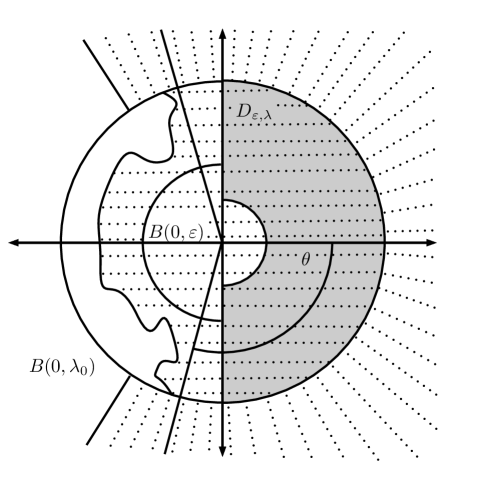
Figure 1. The ball $B(0,\lambda_{0})$ and half of the ball $B(0,\varepsilon)$ are depicted. The gray region visualizes the set $D_{\varepsilon,\lambda}$. Due to the openness of the resolvent set (which is indicated by the dashed region), the spectrum must keep some distance to $D_{\varepsilon,\lambda}$. One sees, that in this constellation one can find a sector $\mathrm{S}_{\theta}$ with $\theta\in(\pi/2,\vartheta)$ that is contained in the resolvent set.

∎

For completeness, let us end the section proving Theorem 1.2. As a start, we apply Theorem 4.1 with $q=1$ and notice that the last step of the proof ensures the existence of some $c>0$ depending only on $\mu,$ $\mu^{\prime}$ and $\Omega$ so that

$$\bigl{\{}z\in\mathbb{C}:\operatorname{Re}(z)\geq-c\bigr{\}}\subset\rho(-A_{p,1,s}).$$

This implies that $A_{p,1,s}+\frac{c}{2}$ has maximal $\mathrm{L}^{1}$-regularity. This yields Inequality (1.5). Of course, Theorem 4.1 directly yields that $(a,u)$ is in $\mathrm{E}_{p}.$

To add non-zero initial data $(a_{0},u_{0})\in\mathcal{X}^{s}_{p,1}$ in problem (1.3) we cannot simply employ Corollary 2.8. The reason is that we would need to choose a ground space $\mathcal{X}^{t}_{p,1}$ for some $t$ slightly smaller than $s$. Then we would need to calculate the real interpolation space $(\mathcal{X}^{t}_{p,1},\mathcal{D}(A_{p,1,t}))_{\theta,1}$. However, as the first components of $\mathcal{X}^{t}_{p,1}$ and $\mathcal{D}(A_{p,1,t})$ are the same, the result of the real interpolation in this first component will be the very same space and thus we will not reach initial data in $\mathcal{X}^{s}_{p,1}$.

To circumvent this problem, consider the caloric extension

$$\begin{pmatrix}a_{c}(t)\\ u_{c}(t)\end{pmatrix}:=\begin{pmatrix}\mathrm{e}^{t\Delta_{N}}a_{0}\\ \mathrm{e}^{t\Delta_{D}}u_{0}\end{pmatrix}\cdotp$$

Here, $\Delta_{N}$ denotes the Neumann Laplacian on $\mathrm{B}^{s+1}_{p,1}(\Omega)\cap\mathrm{L}^{p}_{0}(\Omega)$ and $\Delta_{D}$ denotes the Dirichlet Laplacian on $\mathrm{B}^{s}_{p,1}(\Omega;\mathbb{C}^{d})$. Notice that both operators are invertible and that $\Delta_{N}$ generates a bounded analytic semigroup on $\mathrm{L}^{p}_{0}(\Omega)$ while $\Delta_{D}$ generates a bounded analytic semigroup on $\mathrm{W}^{-1,p}(\Omega;\mathbb{C}^{d})$. An application of Corollary 2.8 yields the existence of a constant $C>0$ such that

$$\|\partial_{t}a_{c},a_{c},\nabla^{2}a_{c}\|_{\mathrm{L}^{1}(\mathbb{R}_{+};\mathrm{B}^{s+1}_{p,1})}+\|\partial_{t}u_{c},u_{c},\nabla^{2}u_{c}\|_{\mathrm{L}^{1}(\mathbb{R}_{+};\mathrm{B}^{s}_{p,1})}\leq C\|(a_{0},u_{0})\|_{\mathcal{X}^{s}_{p,1}}.$$

Notice that this together with the boundedness of the gradient operator between $\mathrm{B}^{s+1}_{p,1}(\Omega)$ and $\mathrm{B}^{s}_{p,1}(\Omega;\mathbb{C}^{d})$ implies that

$$\|\nabla a_{c}\|_{\mathrm{L}^{1}(\mathbb{R}_{+};\mathrm{B}^{s}_{p,1})}\leq C\|a_{c}\|_{\mathrm{L}^{1}(\mathbb{R}_{+};\mathrm{B}^{s+1}_{p,1})}.$$

Now, let $(b,v)\in\mathrm{E}_{p}$ with $(b(0),v(0))=(0,0)$ solve

$$\partial_{t}\begin{pmatrix}b\\ v\end{pmatrix}+A_{p,1,s}\begin{pmatrix}b\\ v\end{pmatrix}=-\partial_{t}\begin{pmatrix}a_{c}\\ u_{c}\end{pmatrix}-A_{p,1,s}\begin{pmatrix}a_{c}\\ u_{c}\end{pmatrix}\in\mathrm{L}^{1}(\mathbb{R}_{+};\mathcal{X}^{s}_{p,1}).$$

Then, for $a:=b+a_{c}$ and $u:=v+u_{c}$ one has $(a,u)\in\mathrm{E}_{p}$ and $(a,u)$ solve (1.3) with $f$ and $g$ being zero and non-zero initial data. ∎

5. Global well-posedness for the compressible Navier–Stokes system

The fastest way to solve System (1.1) in the critical regularity setting is to recast it in Lagrangian coordinates. To this end, let $X$ be the flow associated to $u,$ that is the solution to

(5.1) $$X(t,y)=y+\int_{0}^{t}u(\tau,X(\tau,y))\,\mathrm{d}\tau.$$

The ‘Lagrangian’ density and velocity are defined by

(5.2) $$\bar{\rho}(t,y):=\rho(t,X(t,y))\quad\hbox{and}\quad\bar{u}(t,y):=u(t,X(t,y)).$$

With this notation, relation (5.1) becomes

(5.3) $$X_{\bar{u}}(t,y):=X(t,y)=y+\int_{0}^{t}\bar{u}(\tau,y)\,\mathrm{d}\tau,$$

and thus

(5.4) $$DX_{\bar{u}}(t,y)=\operatorname{Id}+\int_{0}^{t}D\bar{u}(\tau,y)\,\mathrm{d}\tau.$$

The main interest of Lagrangian coordinates is that, whenever $DX_{\bar{u}}(t,y)$ is invertible, the density is entirely determined by $X_{\bar{u}}$ and $\rho_{0}$ through the relation

(5.5) $$\bar{\rho}(t,y)J_{\bar{u}}(t,y)=\rho_{0}(y)\quad\hbox{with}\quad J_{\bar{u}}(t,y):=\det(DX_{\bar{u}}(t,y)).$$

Furthermore, one can write

$$A_{\bar{u}}(t,y):=(DX_{\bar{u}}(t,y))^{-1}=J_{\bar{u}}^{-1}(t,y)\,\operatorname{adj}(DX_{\bar{u}}(t,y))$$

where $\operatorname{adj}(DX_{\bar{u}})$ (the adjugate matrix) stands for the transpose of the comatrix of $DX_{\bar{u}}(t,y).$ Define the ‘twisted’ deformation tensor and divergence operator by

$$D_{A}(z):=\frac{1}{2}\Bigl{(}Dz\cdot A+{}^{T}\!A\cdot\nabla z\Bigr{)}\quad\hbox{and}\quad\operatorname{div_{A}}z:={}^{T}\!A:\nabla z=Dz:A,\quad\bigl{(}A\in\mathbb{R}^{d}\times\mathbb{R}^{d}\bigr{)}\cdotp$$

As shown in, e.g., [9], in terms of the unknowns $\bar{a}:=\bar{\rho}-1$ and $\bar{u},$ System (1.1) translates into

(5.6) $$\left\{\begin{aligned} &J_{\bar{u}}\partial_{t}\bar{a}+(1+\bar{a})D\bar{u}:\operatorname{adj}(DX_{\bar{u}})=0\quad&\hbox{in }\ \mathbb{R}_{+}\times\Omega,\\ &\rho_{0}\partial_{t}\bar{u}-2\operatorname{div}\bigl{(}\mu(1+\bar{a})\operatorname{adj}(DX_{\bar{u}})\cdot D_{A_{\bar{u}}}(\bar{u})\bigr{)}-\nabla\bigl{(}\lambda(1+\bar{a})\operatorname{div}_{A_{\bar{u}}}\bar{u}\bigr{)}&\\ &\hskip 156.49014pt+{}^{T}\!\!\operatorname{adj}(DX_{\bar{u}})\cdot\nabla(P(1+\bar{a}))=0&\quad\hbox{in }\ \mathbb{R}_{+}\times\Omega,\\ &\bar{u}=0&\quad\hbox{on }\ \mathbb{R}_{+}\times\partial\Omega,\\ &(\bar{a},\bar{u})|_{t=0}=(a_{0},u_{0})&\quad\hbox{in }\ \Omega.\end{aligned}\right.$$

As pointed out in the Appendix of [9] (for $\mathbb{R}^{d}$ but the proof in the bounded domain case is similar), in our functional framework, there exists $\varepsilon>0$ such that whenever

(5.7) $$\int_{0}^{T}\|\nabla u\|_{\mathrm{B}^{d/p}_{p,1}(\Omega)}\,\mathrm{d}t\leq\varepsilon,$$

the Eulerian and Lagrangian formulations of the compressible Navier–Stokes equations are equivalent on $[0,T].$

The present section aims at proving a global existence result for small $(a_{0},u_{0})$ in the case $P^{\prime}(1)>0.$ Note that, after rescaling the time and velocity according to (4.1), System (5.6) may be rewritten exactly as (4.5) with

$$f :=(1-J_{\bar{u}})\partial_{t}\bar{a}+D\bar{u}:(\operatorname{Id}-\operatorname{adj}(DX_{\bar{u}}))-\bar{a}D\bar{u}:\operatorname{adj}(DX_{\bar{u}}),$$

$$g :=-a_{0}\partial_{t}\bar{u}+2\operatorname{div}\bigl{(}\widetilde{\mu}(\bar{a})\operatorname{adj}(DX_{\bar{u}})\cdot D_{A_{\bar{u}}}(\bar{u})-\bar{\mu}D(\bar{u})\bigr{)}$$

$$\hskip 85.35826pt+\nabla\bigl{(}(\widetilde{\lambda}(\bar{a})\operatorname{div}_{\!A_{\bar{u}}}\bar{u}-\bar{\lambda}\operatorname{div}\bar{u})\bigr{)}+(1-\Pi(\bar{a}))\nabla\bar{a}+\Pi(\bar{a})(\operatorname{Id}-\operatorname{adj}(DX_{\bar{u}}))\cdot\nabla\bar{a}.$$

Above, we denoted $\widetilde{\mu}(z):=\mu(1+z),$ $\widetilde{\lambda}(z):=\lambda(1+z),$ $\Pi(z):=P^{\prime}(1+z),$ $\bar{\mu}:=\mu(1)$ and $\bar{\lambda}:=\lambda(1).$

In the critical regularity setting, if we restrict ourselves to small perturbations of $(0,0),$ then one can expect $f$ and $g$ (that contain only at least quadratic terms) to be even smaller. Hence, it looks reasonable to get a global existence result for (5.6) by taking advantage of our estimates for the linearized system. From the linear theory, we have the constraint $d/p-1<1/p$ (that is $p>d-1$) and, when handling the nonlinear terms, the additional conditions $p<2d$ and $d\geq 2$ will pop up. In the end, we will obtain the following result, that is the counterpart of Theorem 1.3, in Lagrangian coordinates. Recall that $\mathrm{E}_{p}$ was defined by

$$\mathrm{E}_{p}=\mathrm{W}^{1,1}(\mathbb{R}_{+};\mathrm{B}^{{d}/{p}}_{p,1}(\Omega)\times\mathrm{B}^{{d}/{p}-1}_{p,1}(\Omega;\mathbb{R}^{d}))\cap\mathrm{L}^{1}(\mathbb{R}_{+};\mathrm{B}^{{d}/{p}}_{p,1}(\Omega)\times\mathrm{B}^{{d}/{p}+1}_{p,1}(\Omega;\mathbb{R}^{d}))\cdotp$$

Proposition 5.1.

Let the assumptions of Theorem 1.3 be in force. Then, System (5.6) admits a unique global solution $(\bar{a},\bar{u})$ in the maximal regularity space $\mathrm{E}_{p},$ and there exist two positive constants $c$ and $C$ depending only on the parameters of the system, on $p$, and on $\Omega,$ such that

(5.8) $$\|\mathrm{e}^{ct}(\bar{a},\bar{u})\|_{\mathrm{E}_{p}}\leq C\bigl{(}\|a_{0}\|_{\mathrm{B}^{d/p}_{p,1}}+\|u_{0}\|_{\mathrm{B}^{d/p-1}_{p,1}}\bigr{)}\cdotp$$

Proof.

Throughout, we use the short notation ${\bf A}$ for ${A_{p,1,d/p-1}}.$ The proof of existence is based on the fixed point theorem in the space $\mathrm{E}_{p}^{c}$ defined by

$$\mathrm{E}_{p}^{c}:=\bigl{\{}(a,u):\mathbb{R}_{+}\times\Omega\to\mathbb{R}\times\mathbb{R}^{d}\ \hbox{ s.t. }\ (\mathrm{e}^{tc}a,\mathrm{e}^{tc}u)\in\mathrm{E}_{p}\bigr{\}}$$

for the map $\Phi:({\bar{b}},{\bar{v}})\mapsto({\bar{a}},{\bar{u}}),$ where $({\bar{a}},{\bar{u}})$ stands for the solution in $\mathrm{E}_{p}^{c}$ to the linear system

(5.9) $$\tfrac{\mathrm{d}}{\mathrm{d}t}\begin{pmatrix}{\bar{a}}\\ {\bar{u}}\end{pmatrix}+{\bf A}\begin{pmatrix}{\bar{a}}\\ {\bar{u}}\end{pmatrix}=\begin{pmatrix}{\bar{f}}\\ {\bar{g}}\end{pmatrix}$$

supplemented with initial data $(a_{0},u_{0})$ and

$${\bar{f}} :=(1-J_{{\bar{v}}})\partial_{t}{\bar{b}}+D{\bar{v}}:(\operatorname{Id}-\operatorname{adj}(DX_{\bar{v}}))-{\bar{b}}D{\bar{v}}:\operatorname{adj}(DX_{\bar{v}}),$$

$${\bar{g}} :=-a_{0}\partial_{t}{\bar{v}}+2\operatorname{div}\bigl{(}\widetilde{\mu}({\bar{b}})\operatorname{adj}(DX_{\bar{v}})\cdot D_{A_{\bar{v}}}({\bar{v}})-\bar{\mu}D({\bar{v}})\bigr{)}$$

$$\hskip 56.9055pt+\nabla\bigl{(}(\widetilde{\lambda}({\bar{b}})\operatorname{div}_{A_{\bar{v}}}{\bar{v}}-\bar{\lambda}\operatorname{div}{\bar{v}})\bigr{)}+(1-\Pi({\bar{b}}))\nabla{\bar{b}}+\Pi({\bar{b}})(\operatorname{Id}-\operatorname{adj}(DX_{\bar{v}}))\cdot\nabla{\bar{b}}.$$

We claim that there exists some $R\in(0,1)$ such that, whenever $({\bar{b}},{\bar{v}})$ belongs to the closed ball $\bar{B}_{\mathrm{E}_{p}^{c}}(0,R):=\{(b,v)\in\mathrm{E}_{p}^{c}:\|(b,v)\|_{\mathrm{E}_{p}^{c}}\leq R\},$ System (5.9) admits a solution in $\bar{B}_{\mathrm{E}_{p}^{c}}(0,R).$ Now, from Theorem 4.1, we gather that there exists some $c>0$ depending only on $\Omega,$ $p,$ $\mu$ and $\mu^{\prime}$ such that

(5.10) $$\|(\bar{a},\bar{u})\|_{\mathrm{E}_{p}^{c}}\lesssim\|(a_{0},u_{0})\|_{\mathcal{X}^{d/p-1}_{p,1}}+\|\mathrm{e}^{ct}({\bar{f}},{\bar{g}})\|_{\mathrm{L}^{1}(\mathbb{R}_{+};{\mathcal{X}^{d/p-1}_{p,1}})}.$$

Hence our problem reduces to proving suitable estimates for ${\bar{f}}$ and ${\bar{g}}.$ To this end, we need the following two results proved in Appendix:

Proposition 5.2.

The numerical product is continuous from $\mathrm{B}^{s}_{p,1}(\Omega)\times\mathrm{B}^{d/p}_{p,1}(\Omega)$ to $\mathrm{B}^{s}_{p,1}(\Omega)$ whenever $-\min(d/p,d/p^{\prime})<s\leq d/p.$

Proposition 5.3.

Let $K:\mathbb{R}\to\mathbb{R}$ be a smooth function vanishing at $0,$ and $p\in[1,\infty).$ Then, there exists $C>0$ such that for all functions $z$ belonging to $\mathrm{B}^{d/p}_{p,1}(\Omega),$ the function $K(z)$ belongs to $\mathrm{B}^{d/p}_{p,1}(\Omega)$ and satisfies

$$\|K(z)\|_{\mathrm{B}^{d/p}_{p,1}(\Omega)}\leq C(1+\|z\|_{\mathrm{B}^{d/p}_{p,1}(\Omega)})^{k}\|z\|_{\mathrm{B}^{d/p}_{p,1}(\Omega)}\quad\hbox{with}\quad k:=\lceil d/p\rceil.$$

Furthermore (without assuming $K(0)=0$), for all pairs $(z_{1},z_{2})$ of functions in $\mathrm{B}^{d/p}_{p,1}(\Omega),$ we have

$$\|K(z_{2})-K(z_{1})\|_{\mathrm{B}^{d/p}_{p,1}(\Omega)}\leq C(1+\|z_{1}\|_{\mathrm{B}^{d/p}_{p,1}(\Omega)}+\|z_{2}\|_{\mathrm{B}^{d/p}_{p,1}(\Omega)})^{k}\|z_{2}-z_{1}\|_{\mathrm{B}^{d/p}_{p,1}(\Omega)}\quad\hbox{with}\quad k:=\lceil d/p\rceil.$$

For notational simplicity, we omit from now on the dependency on $\Omega$ in the norms. Assume that $R$ has been chosen so small as

(5.11) $$\|D{\bar{v}}\|_{\mathrm{L}^{1}(\mathbb{R}_{+};\mathrm{B}^{d/p}_{p,1})}\leq\varepsilon\ll 1.$$

In particular, owing to the embedding

(5.12) $$\mathrm{B}^{d/p}_{p,1}(\Omega)\hookrightarrow\mathrm{L}^{\infty}(\Omega),$$

the range of ${\bar{b}}$ is included in a small neighborhood of $0$ and the functions $\widetilde{\mu},$ $\widetilde{\lambda}$, and $\Pi$ may thus be extended smoothly to the whole $\mathbb{R}$ without changing the value of ${\bar{g}}$. This allows to apply Proposition 5.3 whenever it is needed.

Now, decompose ${\bar{f}}$ into

$${\bar{f}} =(1-J_{\bar{v}})\partial_{t}{\bar{b}}+D{\bar{v}}:(\operatorname{Id}-\operatorname{adj}(DX_{\bar{v}}))-{\bar{b}}\,D{\bar{v}}:\operatorname{adj}(DX_{\bar{v}})$$

$$={\bar{f}}^{1}+{\bar{f}}^{2}+{\bar{f}}^{3}.$$

Proposition 5.2 ensures that the space $\mathrm{B}^{d/p}_{p,1}$ is stable under products. Hence

$$\|{\bar{f}}^{1}\|_{\mathrm{B}^{d/p}_{p,1}} \lesssim\|1-J_{\bar{v}}\|_{\mathrm{B}^{d/p}_{p,1}}\|\partial_{t}\bar{b}\|_{\mathrm{B}^{d/p}_{p,1}},$$

$$\|{\bar{f}}^{2}\|_{\mathrm{B}^{d/p}_{p,1}} \lesssim\|D{\bar{v}}\|_{\mathrm{B}^{d/p}_{p,1}}\|\operatorname{Id}-\operatorname{adj}(DX_{\bar{v}})\|_{\mathrm{B}^{d/p}_{p,1}},$$

$$\|{\bar{f}}^{3}\|_{\mathrm{B}^{d/p}_{p,1}} \lesssim\|{\bar{b}}\|_{\mathrm{B}^{d/p}_{p,1}}\|D{\bar{v}}\|_{\mathrm{B}^{d/p}_{p,1}}\bigl{(}1+\|\operatorname{Id}-\operatorname{adj}(DX_{\bar{v}})\|_{\mathrm{B}^{d/p}_{p,1}}\bigr{)}\cdotp$$

In order to bound the right-hand sides (as well as the terms in ${\bar{g}}$ below), we will use repeatedly the following inequality that is based on Neumann expansion arguments, (5.11) and on the fact that $\mathrm{B}^{d/p}_{p,1}$ is stable under products (see details in the Appendix of [9] for the $\mathbb{R}^{d}$ situation):

(5.13) $$\sup_{t\geq 0}\Bigl{(}\|1-J_{\bar{v}}(t)\|_{\mathrm{B}^{d/p}_{p,1}}+\|A_{\bar{v}}(t)-\operatorname{Id}\|_{\mathrm{B}^{d/p}_{p,1}}+\|\operatorname{adj}(DX_{\bar{v}}(t))-\operatorname{Id}\|_{\mathrm{B}^{d/p}_{p,1}}\Bigr{)}\lesssim\|D{\bar{v}}\|_{\mathrm{L}^{1}(\mathbb{R}_{+};\mathrm{B}^{d/p}_{p,1})}.$$

In the end, we get

(5.14) $$\|\mathrm{e}^{ct}{\bar{f}}\|_{\mathrm{L}^{1}(\mathbb{R}_{+};\mathrm{B}^{d/p}_{p,1})}\lesssim\bigl{(}\|\mathrm{e}^{ct}\partial_{t}{\bar{b}}\|_{\mathrm{L}^{1}(\mathbb{R}_{+};\mathrm{B}^{d/p}_{p,1})}\\ +(1+\|D{\bar{v}}\|_{\mathrm{L}^{\infty}(\mathbb{R}_{+};\mathrm{B}^{d/p}_{p,1})})\|\mathrm{e}^{ct}{\bar{b}}\|_{\mathrm{L}^{\infty}(\mathbb{R}_{+};\mathrm{B}^{d/p}_{p,1})}+\|\mathrm{e}^{ct}D{\bar{v}}\|_{\mathrm{L}^{1}(\mathbb{R}_{+};\mathrm{B}^{d/p}_{p,1})}\bigr{)}\|D{\bar{v}}\|_{\mathrm{L}^{1}(\mathbb{R}_{+};\mathrm{B}^{d/p}_{p,1})}.$$

Next, we have to bound in $\mathrm{L}^{1}(\mathbb{R}_{+};\mathrm{B}^{d/p-1}_{p,1})$ the five terms constituting ${\bar{g}},$ namely

$$\begin{array}[]{ll}{\bar{g}}^{1}:=-a_{0}\partial_{t}{\bar{v}},&\quad{\bar{g}}^{2}:=2\operatorname{div}\bigl{(}\widetilde{\mu}({\bar{b}})\operatorname{adj}(DX_{\bar{v}})\cdot D_{A_{\bar{v}}}({\bar{v}})-\bar{\mu}D({\bar{v}})\bigr{)},\\[6.45831pt] {\bar{g}}^{3}:=\nabla\bigl{(}(\widetilde{\lambda}({\bar{b}})\operatorname{div}_{A_{\bar{v}}}{\bar{v}}-\bar{\lambda}\operatorname{div}{\bar{v}})\bigr{)},&\quad{\bar{g}}^{4}:=(1-\Pi({\bar{b}}))\nabla{\bar{b}},\\[6.45831pt] {\bar{g}}^{5}:=\Pi({\bar{b}})(\operatorname{Id}-\operatorname{adj}(DX_{\bar{v}}))\cdot\nabla{\bar{b}}.&\end{array}$$

For ${\bar{g}}^{1},$ a direct application of Proposition 5.2 yields, provided $p<2d$ and $d\geq 2,$

(5.15) $$\|\mathrm{e}^{ct}{\bar{g}}^{1}\|_{\mathrm{L}^{1}(\mathbb{R}_{+};\mathrm{B}^{d/p-1}_{p,1})}\lesssim\|a_{0}\|_{\mathrm{B}^{d/p}_{p,1}}\|\mathrm{e}^{ct}\partial_{t}{\bar{v}}\|_{\mathrm{L}^{1}(\mathbb{R}_{+};\mathrm{B}^{d/p-1}_{p,1})}.$$

Similarly, combining Propositions 5.2 and 5.3 yields

$$\|\mathrm{e}^{ct}{\bar{g}}^{4}\|_{\mathrm{L}^{1}(\mathbb{R}_{+};\mathrm{B}^{d/p-1}_{p,1})}\lesssim\|\mathrm{e}^{ct}{\bar{b}}\|_{\mathrm{L}^{\infty}(\mathbb{R}_{+};\mathrm{B}^{d/p}_{p,1})}\|\nabla{\bar{b}}\|_{\mathrm{L}^{1}(\mathbb{R}_{+};\mathrm{B}^{d/p-1}_{p,1})}$$

and since (argue by extension)

(5.16) $$\nabla:\mathrm{B}^{s+1}_{p,1}(\Omega)\to\mathrm{B}^{s}_{p,1}(\Omega)\quad\text{is a bounded operator},$$

one can conclude that

(5.17) $$\|\mathrm{e}^{ct}{\bar{g}}^{4}\|_{\mathrm{L}^{1}(\mathbb{R}_{+};\mathrm{B}^{d/p-1}_{p,1})}\lesssim\|\mathrm{e}^{ct}{\bar{b}}\|_{\mathrm{L}^{\infty}(\mathbb{R}_{+};\mathrm{B}^{d/p}_{p,1})}\|{\bar{b}}\|_{\mathrm{L}^{1}(\mathbb{R}_{+};\mathrm{B}^{d/p}_{p,1})}.$$

To handle ${\bar{g}}^{2}$, we use the decomposition

$${\bar{g}}^{2}=2\operatorname{div}\Bigl{(}(\widetilde{\mu}({\bar{b}})-\bar{\mu})\operatorname{adj}(DX_{\bar{v}})\cdot D_{A_{\bar{v}}}({\bar{v}})+\bar{\mu}(\operatorname{adj}(DX_{\bar{v}})-\operatorname{Id})\cdot D_{A_{\bar{v}}}({\bar{v}})+\bar{\mu}(D_{A_{\bar{v}}}({\bar{v}})-D({\bar{v}}))\Bigr{)}\cdotp$$

From the definition of $D_{A_{\bar{v}}},$ (5.11) and (5.13), we gather that

$$\|\mathrm{e}^{ct}(D_{A_{\bar{v}}}({\bar{v}})-D({\bar{v}}))\|_{\mathrm{L}^{1}(\mathbb{R}_{+};\mathrm{B}^{d/p}_{p,1})}\lesssim\|\mathrm{e}^{ct}D{\bar{v}}\|_{\mathrm{L}^{1}(\mathbb{R}_{+};\mathrm{B}^{d/p}_{p,1})}\|D{\bar{v}}\|_{\mathrm{L}^{1}(\mathbb{R}_{+};\mathrm{B}^{d/p}_{p,1})}.$$

Hence, combining with Propositions 5.2 and 5.3, (5.13) and (5.16), as (5.11) is fulfilled, we get

(5.18) $$\|\mathrm{e}^{ct}{\bar{g}}^{2}\|_{\mathrm{L}^{1}(\mathbb{R}_{+};\mathrm{B}^{d/p-1}_{p,1})}\lesssim\bigl{(}1+\|{\bar{b}}\|_{\mathrm{L}^{\infty}(\mathbb{R}_{+};\mathrm{B}^{d/p}_{p,1})}\bigr{)}\|\mathrm{e}^{ct}D{\bar{v}}\|_{\mathrm{L}^{1}(\mathbb{R}_{+};\mathrm{B}^{d/p}_{p,1})}\|D{\bar{v}}\|_{\mathrm{L}^{1}(\mathbb{R}_{+};\mathrm{B}^{d/p}_{p,1})}.$$

Bounding ${\bar{g}}^{3}$ is exactly the same. Finally, we have

$${\bar{g}}^{5}=\bigl{(}1+(\Pi({\bar{b}})-1)\bigr{)}(\operatorname{Id}-\operatorname{adj}(DX_{\bar{v}}))\cdot\nabla{\bar{b}}$$

and thus, combining Propositions 5.2 and 5.3 with (5.16), one ends up with

(5.19) $$\|\mathrm{e}^{ct}{\bar{g}}^{5}\|_{\mathrm{L}^{1}(\mathbb{R}_{+};\mathrm{B}^{d/p-1}_{p,1})}\lesssim\bigl{(}1+\|{\bar{b}}\|_{\mathrm{L}^{\infty}(\mathbb{R}_{+};\mathrm{B}^{d/p}_{p,1})}\bigr{)}\|D{\bar{v}}\|_{\mathrm{L}^{1}(\mathbb{R}_{+};\mathrm{B}^{d/p}_{p,1})}\|\mathrm{e}^{ct}{\bar{b}}\|_{\mathrm{L}^{1}(\mathbb{R}_{+};\mathrm{B}^{d/p}_{p,1})}.$$

Recall that the embedding $\mathrm{W}^{1,1}(\mathbb{R}_{+};\mathrm{B}^{{d}/{p}}_{p,1})\hookrightarrow\mathrm{L}^{\infty}(\mathbb{R}_{+};\mathrm{B}^{{d}/{p}}_{p,1})$ allows to control the $\mathrm{L}^{\infty}$-norms of quantities involving ${\bar{b}}$ by their norm in $\mathrm{E}_{p}$. Now, plugging Inequalities (5.14), (5.15), (5.17), (5.18), and (5.19) in (5.10) and using the definition of the norm in $\mathrm{E}_{p}$ yields

$$\|\mathrm{e}^{ct}({\bar{a}},{\bar{u}})\|_{\mathrm{E}_{p}}\leq C\Bigl{(}\|(a_{0},u_{0})\|_{\mathcal{X}^{d/p-1}_{p,1}}+(1+\|({\bar{b}},{\bar{v}})\|_{\mathrm{E}_{p}})\|({\bar{b}},{\bar{v}})\|_{\mathrm{E}_{p}}\|\mathrm{e}^{ct}({\bar{b}},{\bar{v}})\|_{\mathrm{E}_{p}}\Bigr{)}\cdotp$$

Remembering (1.6) and $({\bar{b}},{\bar{v}})\in\bar{B}_{\mathrm{E}_{p}^{c}}(0,R)$ with $R\in(0,1),$ one thus gets up to a change of $C,$

$$\|({\bar{a}},{\bar{u}})\|_{\mathrm{E}_{p}^{c}}\leq C(\alpha+R^{2}).$$

Therefore, choosing $R=2C\alpha$ and assuming that $4C\alpha\leq 1,$ one can conclude that $({\bar{a}},{\bar{u}})\in\bar{B}_{\mathrm{E}_{p}^{c}}(0,R).$

To complete the proof of existence of a fixed point for $\Phi,$ it is only a matter of exhibiting its properties of contraction. So let us consider $({\bar{b}}_{i},{\bar{v}}_{i})\in\bar{B}_{\mathrm{E}_{p}^{c}}(0,R)$ and $({\bar{a}}_{i},{\bar{u}}_{i}):=\Phi({\bar{b}}_{i},{\bar{v}}_{i}),$ $i=1,2.$ Denote $({\bar{f}}_{i},{\bar{g}}_{i}),$ $i=1,2$ the right-hand sides of System (5.9) corresponding to $({\bar{b}}_{i},{\bar{v}}_{i}).$ Then, from Theorem 1.2, we gather

(5.20) $$\|(\delta\!a,\delta\!u)\|_{\mathrm{E}_{p}^{c}}\lesssim\|\mathrm{e}^{ct}(\delta\!f,\delta\!g)\|_{\mathrm{L}^{1}(\mathbb{R}_{+};{\mathcal{X}^{d/p-1}_{p,1}})},$$

where $\delta\!a:={\bar{a}}_{2}-{\bar{a}}_{1},$ $\delta\!u:={\bar{u}}_{2}-{\bar{u}}_{1},$ $\delta\!f:={\bar{f}}_{2}-{\bar{f}}_{1}$, and $\delta\!g:={\bar{g}}_{2}-{\bar{g}}_{1}.$

Let us use the short notation $\operatorname{div}_{i}:=\operatorname{div}_{v_{i}}$ and so on and also introduce $\delta\!b:={\bar{b}}_{2}-{\bar{b}}_{1}$ and $\delta\!v:={\bar{v}}_{2}-{\bar{v}}_{1}$. We see that

$$\delta\!f^{1} =(1-J_{1})\partial_{t}\delta\!b+(J_{1}-J_{2})\partial_{t}{\bar{b}}_{2},$$

$$\delta\!f^{2} =D{\bar{v}}_{1}:\bigl{(}\operatorname{adj}(DX_{1})-\operatorname{adj}(DX_{2})\bigr{)}+D\delta\!v:(\operatorname{Id}-\operatorname{adj}(DX_{2})),$$

$$\delta\!f^{3} ={\bar{b}}_{1}\bigl{(}D{\bar{v}}_{1}:(\operatorname{adj}(DX_{1})-\operatorname{adj}(DX_{2}))-D\delta\!v:\operatorname{adj}(DX_{2})\bigr{)}-\delta\!b\,D{\bar{v}}_{2}:\operatorname{adj}(DX_{2}).$$

Since we have

$$A_{2}(t)-A_{1}(t)=\sum_{k=1}^{\infty}(-1)^{k}\sum_{j=0}^{k-1}\biggl{(}\int_{0}^{t}D{\bar{v}}_{2}\,\mathrm{d}\tau\biggr{)}^{j}\biggl{(}\int_{0}^{t}D\delta\!v\,\mathrm{d}\tau\biggr{)}\biggl{(}\int_{0}^{t}D{\bar{v}}_{1}\,\mathrm{d}\tau\biggr{)}^{k-1-j}$$

and similar identities for $J_{2}(t)-J_{1}(t)$ and $\operatorname{adj}(DX_{2}(t))-\operatorname{adj}(DX_{1}(t)),$ we get thanks to the stability of $\mathrm{B}^{d/p}_{p,1}$ under multiplication and to (5.11) (remember that $R$ is small) that for all $t\geq 0,$

(5.21) $$\|A_{2}(t)-A_{1}(t)\|_{\mathrm{B}^{d/p}_{p,1}}+\|\operatorname{adj}(DX_{2}(t))-\operatorname{adj}(DX_{1}(t))\|_{\mathrm{B}^{d/p}_{p,1}}\\ +\|J_{2}^{\pm 1}(t)-J_{1}^{\pm 1}(t)\|_{\mathrm{B}^{d/p}_{p,1}}\lesssim\|D\delta\!v\|_{\mathrm{L}^{1}(\mathbb{R}_{+};\mathrm{B}^{d/p}_{p,1})}.$$

Hence, using once more the stability of $\mathrm{B}^{d/p}_{p,1}$ under multiplication eventually yields

(5.22) $$\|\mathrm{e}^{ct}\delta\!f\|_{\mathrm{L}^{1}(\mathbb{R}_{+};\mathrm{B}^{d/p}_{p,1})}\lesssim\bigl{(}\|D{\bar{v}}_{1}\|_{\mathrm{L}^{1}(\mathbb{R}_{+};\mathrm{B}^{d/p}_{p,1})}+\|D{\bar{v}}_{2}\|_{\mathrm{L}^{1}(\mathbb{R}_{+};\mathrm{B}^{d/p}_{p,1})}\\ +\|\partial_{t}{\bar{b}}_{2}\|_{\mathrm{L}^{1}(\mathbb{R}_{+};\mathrm{B}^{{d}/{p}}_{p,1})}+\|{\bar{b}}_{1}\|_{\mathrm{L}^{\infty}(\mathbb{R}_{+};\mathrm{B}^{{d}/{p}}_{p,1})}\bigr{)}\cdot\bigl{(}\|\mathrm{e}^{ct}D\delta\!v\|_{\mathrm{L}^{1}(\mathbb{R}_{+};\mathrm{B}^{d/p}_{p,1})}+\|\mathrm{e}^{ct}\partial_{t}\delta\!b\|_{\mathrm{L}^{1}(\mathbb{R}_{+};\mathrm{B}^{{d}/{p}}_{p,1})}\bigr{)}.$$

We compute:

$$\delta\!g^{1} :=-a_{0}\partial_{t}\delta\!v,$$

$$\delta\!g^{2} :=2\operatorname{div}\Bigl{(}(\widetilde{\mu}({\bar{b}}_{2})-\widetilde{\mu}({\bar{b}}_{1}))\operatorname{adj}(DX_{2})\cdot D_{A_{2}}({\bar{v}}_{2})$$

$$+\widetilde{\mu}({\bar{b}}_{1})\bigl{(}\bigl{(}\operatorname{adj}(DX_{1})-\operatorname{Id}\bigr{)}\cdot\bigl{(}D_{A_{2}}({\bar{v}}_{2})-D_{A_{1}}({\bar{v}}_{1})\bigr{)}+\bigl{(}\operatorname{adj}(DX_{2})-\operatorname{adj}(DX_{1})\bigr{)}\cdot D_{A_{2}}(v_{2})\bigr{)}$$

$$\qquad\qquad+(\widetilde{\mu}({\bar{b}}_{1})-\bar{\mu})\bigl{(}D_{A_{2}}({\bar{v}}_{2})-D_{A_{1}}({\bar{v}}_{1})\bigr{)}+\bar{\mu}\bigl{(}D_{A_{2}}({\bar{v}}_{2})-D_{A_{1}}({\bar{v}}_{1})-D(\delta\!v)\bigr{)}\Bigr{)},$$

$$\delta\!g^{3} :=\nabla\Bigl{(}\bigl{(}\widetilde{\lambda}({\bar{b}}_{2})-\widetilde{\lambda}({\bar{b}}_{1})\bigr{)}\operatorname{div}_{A_{2}}{\bar{v}}_{2}+\bigl{(}\widetilde{\lambda}({\bar{b}}_{1})-\bar{\lambda}\bigr{)}\bigl{(}\bigl{(}\operatorname{div}_{A_{2}}{\bar{v}}_{2}-\operatorname{div}_{A_{2}}{\bar{v}}_{1}\bigr{)}$$

$$\qquad\qquad\qquad+\bigl{(}\operatorname{div}_{A_{2}}{\bar{v}}_{1}-\operatorname{div}_{A_{1}}{\bar{v}}_{1}\bigr{)}\bigr{)}+\bar{\lambda}\bigl{(}\operatorname{div}_{A_{2}}{\bar{v}}_{2}-\operatorname{div}_{A_{1}}{\bar{v}}_{1}-\operatorname{div}\delta\!v\bigr{)}\Bigr{)},$$

$$\delta\!g^{4} :=(1-\Pi({\bar{b}}_{1}))\nabla\delta\!b+\bigl{(}\Pi({\bar{b}}_{1})-\Pi({\bar{b}}_{2})\bigr{)}\nabla{\bar{b}}_{2},$$

$$\delta\!g^{5} :=\Pi({\bar{b}}_{1})(\operatorname{Id}-\operatorname{adj}(DX_{1}))\cdot\nabla\delta\!b+\Pi({\bar{b}}_{1})(\operatorname{adj}(DX_{1})-\operatorname{adj}(DX_{2}))\cdot\nabla{\bar{b}}_{2}$$

$$\hskip 199.16928pt+(\Pi({\bar{b}}_{2})-\Pi({\bar{b}}_{1}))(\operatorname{Id}-\operatorname{adj}(DX_{2}))\cdot\nabla{\bar{b}}_{2}.$$

It is straightforward that

(5.23) $$\|\mathrm{e}^{ct}\delta\!g^{1}\|_{\mathrm{B}^{d/p-1}_{p,1}}\leq C\|a_{0}\|_{\mathrm{B}^{d/p}_{p,1}}\|\mathrm{e}^{ct}\partial_{t}\delta\!v\|_{\mathrm{B}^{d/p-1}_{p,1}}.$$

Next, from Propositions 5.2 and 5.3,  (5.16) and Inequality (5.21), we easily get for $i=2,3,4,5,$

$$\|\mathrm{e}^{ct}\delta\!g^{i}\|_{\mathrm{L}^{1}(\mathbb{R}_{+};\mathrm{B}^{d/p-1}_{p,1})} \lesssim\Big{(}\|{\bar{b}}_{2},\nabla{\bar{v}}_{1},\nabla{\bar{v}}_{2}\|_{\mathrm{L}^{1}(\mathbb{R}_{+};\mathrm{B}^{d/p}_{p,1})}+\|{\bar{b}}_{1}\|_{\mathrm{L}^{\infty}(\mathbb{R}_{+};\mathrm{B}^{{d}/{p}}_{p,1})}\Big{)}\|\mathrm{e}^{ct}\delta\!b\|_{\mathrm{L}^{1}(\mathbb{R}_{+};\mathrm{B}^{d/p}_{p,1})}$$

$$\quad+\Big{(}\|{\bar{b}}_{1},{\bar{b}}_{2},\nabla{\bar{v}}_{1},\nabla{\bar{v}}_{2}\|_{\mathrm{L}^{1}(\mathbb{R}_{+};\mathrm{B}^{d/p}_{p,1})}+\|{\bar{b}}_{1}\|_{\mathrm{L}^{\infty}(\mathbb{R}_{+};\mathrm{B}^{d/p}_{p,1})}\Big{)}\|\mathrm{e}^{ct}\delta\!b\|_{\mathrm{L}^{\infty}(\mathbb{R}_{+};\mathrm{B}^{d/p}_{p,1})}$$

$$\quad+\Big{(}\|{\bar{b}}_{1},{\bar{b}}_{2},\nabla{\bar{v}}_{1},\nabla{\bar{v}}_{2}\|_{\mathrm{L}^{1}(\mathbb{R}_{+};\mathrm{B}^{d/p}_{p,1})}+\|{\bar{b}}_{1}\|_{\mathrm{L}^{\infty}(\mathbb{R}_{+};\mathrm{B}^{d/p}_{p,1})}\Big{)}\|\mathrm{e}^{ct}\nabla\delta\!v\|_{\mathrm{L}^{1}(\mathbb{R}_{+};\mathrm{B}^{d/p}_{p,1})}.$$

Note again, that the embedding $\mathrm{W}^{1,1}(\mathbb{R}_{+};\mathrm{B}^{{d}/{p}}_{p,1})\hookrightarrow\mathrm{L}^{\infty}(\mathbb{R}_{+};\mathrm{B}^{{d}/{p}}_{p,1})$ allows to control the $\mathrm{L}^{\infty}$-norms of quantities involving ${\bar{b}}_{1}$ or ${\bar{b}}_{2}$ by their norm in $\mathrm{E}_{p}$. Altogether, we conclude that

$$\|(\delta\!a,\delta\!u)\|_{\mathrm{E}_{p}^{c}}\leq C(R+\alpha)\|(\delta\!b,\delta\!v)\|_{\mathrm{E}_{p}^{c}}.$$

Since we chose $R$ of order $\alpha,$ we see that, indeed, the map $\Phi$ is contracting provided $\alpha$ is small enough. Then, Banach fixed point theorem ensures that $\Phi$ admits a fixed point in $\bar{B}_{\mathrm{E}_{p}^{c}}(0,R).$ Hence, we have a solution for (5.6) with the desired property.

In order to prove the uniqueness, consider two solutions $({\bar{a}}_{1},{\bar{u}}_{1})$ and $({\bar{a}}_{2},{\bar{u}}_{2})$ in $\mathrm{E}_{p}^{c}$ of (5.6) supplemented with the same data $(\rho_{0},u_{0}).$ Then, we have $({\bar{a}}_{i},{\bar{u}}_{i})=\Phi(({\bar{a}}_{i},{\bar{u}}_{i})),$ $i=1,2,$ and one can repeat the previous computation on any interval $[0,T]$ such that

$$\max\biggl{(}\int_{0}^{T}\|\nabla{\bar{u}}_{1}\|_{\mathrm{B}^{d/p}_{p,1}}\,\mathrm{d}t,\int_{0}^{T}\|\nabla{\bar{u}}_{2}\|_{\mathrm{B}^{d/p}_{p,1}}\,\mathrm{d}t\biggr{)}\leq\varepsilon\ll 1.$$

On such an interval, we obtain (with obvious notation)

$$\|(\delta\!a,\delta\!u)\|_{\mathrm{E}_{p}(T)}\leq C\bigl{(}\|({\bar{a}}_{1},{\bar{u}}_{1})\|_{\mathrm{E}_{p}(T)}+\|(\delta\!a,\delta\!u)\|_{\mathrm{E}_{p}(T)}\bigr{)}\|(\delta\!a,\delta\!u)\|_{\mathrm{E}_{p}(T)}.$$

Since the function $t\mapsto\|(\delta\!a,\delta\!u)\|_{\mathrm{E}_{p}(t)}$ is continuous and vanishes at $0$ and because one can assume with no loss of generality that $({\bar{a}}_{1},{\bar{u}}_{1})$ is the small solution constructed just above, we get uniqueness on $[0,T].$ Then, using a standard bootstrap argument yields uniqueness for all time. ∎

6. Local existence for general data with no vacuum

For achieving the local well-posedness of the compressible Navier–Stokes equations, there is no need to take the linear coupling of the density and velocity equations into consideration, and the sign of $P^{\prime}$ does not matter. Actually, in the Lagrangian formulation (5.6), it is enough to solve the velocity equation, since $J_{\bar{u}}\bar{\rho}=\rho_{0}$ and $J_{\bar{u}}$ may be computed from $\bar{u}.$ The pressure may be seen as a source term, and combining Corollary 3.9 with $s=d/p-1$ and $q=1,$ with suitable nonlinear estimates allows to solve (5.6) locally in the critical regularity setting.

Clearly, a basic perturbative method relying on our reference linear system with constant coefficients is bound to fail if the density variations are too large. However, since, in our functional setting, $\rho_{0}$ has to be uniformly continuous in $\Omega,$ one can expect that difficulty to be challengeable if using a suitable localization argument.

Here, for expository purpose, we first present the proof of the local well-posedness in the easier case where $\rho_{0}$ is close to some positive constant. Then, we explain what has to be modified to tackle the general case where one just assumes that it is bounded away from $0.$

6.1. The case of small variations of density

Our goal here is to establish the following result that implies Theorem 1.1 in the case of small density variations.

Proposition 6.1.

Let the assumptions of Theorem 1.1 be in force, and assume in addition that, for a small enough $\alpha>0,$ we have

(6.1) $$\|a_{0}\|_{\mathrm{B}^{d/p}_{p,1}(\Omega)}\leq\alpha.$$

Then, System (5.6) admits a unique solution $(\bar{a},\bar{u})$ on some interval $[0,T],$ such that $1+\bar{a}:=J_{\bar{u}}^{-1}\rho_{0}$ is bounded away from zero on $[0,T]\times\Omega$ and

$$({\bar{a}},{\bar{u}})\in\mathrm{W}^{1,1}(0,T;\mathrm{B}^{d/p}_{p,1}(\Omega)\times\mathrm{B}^{{d}/{p}-1}_{p,1}(\Omega;\mathbb{R}^{d}))\cap\mathrm{L}^{1}(0,T;\mathrm{B}^{{d}/{p}}_{p,1}(\Omega)\times\mathrm{B}^{d/p-1}_{p,1}(\Omega;\mathbb{R}^{d})).$$

Proof.

Throughout, we use the short notation ${\bf L}$ for ${\bf L}_{p,1,d/p-1}.$ Since the variations of density are small, one can look at the velocity equation as follows:

$$\halign{\hbox to\displaywidth{$\hfil\displaystyle#\hfil$}\cr 0.0pt{\hfil$\displaystyle\quad\partial_{t}\bar{u}+{\bf L}\bar{u}=-a_{0}\partial_{t}\bar{u}+2\operatorname{div}\bigl{(}\widetilde{\mu}(\bar{a})\operatorname{adj}(DX_{\bar{u}})\cdot D_{A_{\bar{u}}}(\bar{u})-\bar{\mu}D(\bar{u})\bigr{)}\\ \hfill\cr 0.0pt{\hfil$\displaystyle\hfill+\nabla\bigl{(}(\widetilde{\lambda}(\bar{a})\operatorname{div}_{A_{\bar{u}}}\bar{u}-\bar{\lambda}\operatorname{div}\bar{u})\bigr{)}-{}^{T}\!\operatorname{adj}(DX_{\bar{u}})\cdot\nabla(P(1+\bar{a}))\quad\crcr}}}$$

with $\bar{a}$ given by

$$\bar{a}=J^{-1}_{\bar{u}}\rho_{0}-1=(J^{-1}_{\bar{u}}-1)(1+a_{0})+a_{0}.$$

To proceed, we introduce for $T>0,$ the space

$$\mathrm{F}_{p}(T):=\mathrm{W}^{1,1}(0,T;\mathrm{B}^{{d}/{p}-1}_{p,1}(\Omega;\mathbb{R}^{d}))\cap\mathrm{L}^{1}(0,T;\mathrm{B}^{d/p-1}_{p,1}(\Omega;\mathbb{R}^{d}))\cdotp$$

We consider the map $\Psi:{\bar{v}}\mapsto{\bar{u}}$ where ${\bar{u}}$ is the solution to

$$\partial_{t}\bar{u}+{\bf L}\bar{u}={\bar{h}}\quad\hbox{in }\ (0,T)\times\Omega\quad\hbox{and}\quad u|_{t=0}=u_{0}\ \hbox{ in }\ \Omega,$$

with ${\bar{h}}={\bar{h}}^{1}+{\bar{h}}^{2}+{\bar{h}}^{3}+{\bar{h}}^{4}$ and

$${\bar{h}}^{1}:=-a_{0}\partial_{t}{\bar{v}},\quad {\bar{h}}^{2}:=2\operatorname{div}\bigl{(}\widetilde{\mu}({\bar{b}})\operatorname{adj}(DX_{\bar{v}})\cdot D_{A_{\bar{v}}}({\bar{v}})-\bar{\mu}D({\bar{v}})\bigr{)}$$

$${\bar{h}}^{3}:=\nabla\bigl{(}(\widetilde{\lambda}({\bar{b}})\operatorname{div}_{A_{{\bar{v}}}}{\bar{v}}-\bar{\lambda}\operatorname{div}{\bar{v}})\bigr{)},\quad {\bar{h}}^{4}:=-{}^{T}\!\operatorname{adj}(DX_{\bar{v}})\cdot\nabla(P(1+{\bar{b}}))\cdotp$$

Above, the function ${\bar{b}}$ is defined by

(6.2) $${\bar{b}}=J^{-1}_{\bar{v}}\rho_{0}-1=(J^{-1}_{\bar{v}}-1)(1+a_{0})+a_{0}.$$

We claim that there exists $\alpha>0$ in (6.1) such that for small enough $R,T>0,$ the function $\Psi$ is a self-map on $\bar{B}_{\mathrm{F}_{p}(T)}(u_{L},R),$ where $u_{L}:=\mathrm{e}^{-t{\bf L}}u_{0}$. To justify our claim, we set $\widetilde{v}:={\bar{v}}-u_{L}$ and look for ${\bar{u}}$ under the form ${\bar{u}}:=u_{L}+\widetilde{u}$ with $\widetilde{u}$ satisfying

$$\partial_{t}\widetilde{u}+{\bf L}\widetilde{u}={\bar{h}}\quad\hbox{in }\ (0,T)\times\Omega\quad\hbox{and}\quad\widetilde{u}|_{t=0}=0\ \hbox{ in }\ \Omega.$$

Consequently, Corollary 3.9 yields some $C>0$ independent of $T>0$ such that

(6.3) $$\|\widetilde{u}\|_{\mathrm{F}_{p}(T)}\leq C\|{\bar{h}}\|_{\mathrm{L}^{1}(0,T;\mathrm{B}^{d/p-1}_{p,1})}\quad\hbox{and}\quad\|u_{L}\|_{\mathrm{F}_{p}(T)}\leq C\|u_{0}\|_{\mathrm{B}^{d/p-1}_{p,1}}.$$

By Lebesgue’s dominated convergence theorem, $\|\nabla u_{L}\|_{\mathrm{L}^{1}(0,T;\mathrm{B}^{d/p}_{p,1})}$ converges to $0$ as $T\to 0.$ Hence, for any $R>0,$ one can find $T>0$ so that

(6.4) $$\int_{0}^{T}\|\nabla u_{L}\|_{\mathrm{B}^{d/p}_{p,1}}\,\mathrm{d}t\leq\frac{R}{2}\cdotp$$

Next, we have to bound ${\bar{h}}^{1}$ to ${\bar{h}}^{4}$ in $\mathrm{L}^{1}(0,T;\mathrm{B}^{d/p-1}_{p,1}).$ We shall use repeatedly Proposition 5.2 with $s\in\{d/p,d/p-1\}$ and Proposition 5.3, as well as the local-in-time version of (5.13). First, it is obvious that

$$\|{\bar{h}}^{1}\|_{\mathrm{L}^{1}(0,T;\mathrm{B}^{d/p-1}_{p,1})} \lesssim\|a_{0}\|_{\mathrm{B}^{d/p}_{p,1}}\|\partial_{t}{\bar{v}}\|_{\mathrm{L}^{1}(0,T;\mathrm{B}^{d/p-1}_{p,1})}$$

$$\lesssim\alpha R.$$

In order to bound the next terms, we shall use the fact that, owing to the decomposition of ${\bar{b}}$ in (6.2), the product and composition results in Proposition 5.2 and 5.3, and the local-in-time version of (5.13), we have for all smooth functions $k$ vanishing at $0$ and $t\in[0,T],$

$$\|k({\bar{b}}(t))\|_{\mathrm{B}^{d/p}_{p,1}} \lesssim\|{\bar{b}}(t)\|_{\mathrm{B}^{d/p}_{p,1}}$$

$$\lesssim\|a_{0}\|_{\mathrm{B}^{d/p}_{p,1}}+(1+\|a_{0}\|_{\mathrm{B}^{d/p}_{p,1}})\|J^{-1}_{\bar{v}}(t)-1\|_{\mathrm{B}^{d/p}_{p,1}}$$

$$\lesssim\|a_{0}\|_{\mathrm{B}^{d/p}_{p,1}}+(1+\|a_{0}\|_{\mathrm{B}^{d/p}_{p,1}})\int_{0}^{t}\|\nabla{\bar{v}}\|_{\mathrm{B}^{d/p}_{p,1}}\,\mathrm{d}\tau$$

$$\lesssim\alpha+R.$$

To bound ${\bar{h}}^{2},$ we use the decomposition

$$\halign{\hbox to\displaywidth{$\hfil\displaystyle#\hfil$}\cr 0.0pt{\hfil$\displaystyle\widetilde{\mu}({\bar{b}})\operatorname{adj}(DX_{\bar{v}})\cdot D_{A_{\bar{v}}}({\bar{v}})-\bar{\mu}D({\bar{v}})=(\widetilde{\mu}({\bar{b}})-\bar{\mu})\operatorname{adj}(DX_{\bar{v}})\cdot D_{A_{\bar{v}}}({\bar{v}})\hfill\cr 0.0pt{\hfil$\displaystyle\hfill+\bar{\mu}(\operatorname{adj}(DX_{\bar{v}})-\operatorname{Id})\cdot D_{A_{\bar{v}}}({\bar{v}})+\bar{\mu}(D_{A_{\bar{v}}}({\bar{v}})-D({\bar{v}})).\crcr}}}$$

Hence, using the aforementioned results and also (5.16), we find that for all $t\in[0,T],$

$$\halign{\hbox to\displaywidth{$\hfil\displaystyle#\hfil$}\cr 0.0pt{\hfil$\displaystyle\quad\|{\bar{h}}^{2}\|_{\mathrm{B}^{d/p-1}_{p,1}}\lesssim\|{\bar{b}}\|_{\mathrm{B}^{d/p}_{p,1}}\|\operatorname{adj}(DX_{\bar{v}})\cdot D_{A_{\bar{v}}}({\bar{v}})\|_{\mathrm{B}^{d/p}_{p,1}}\hfill\cr 0.0pt{\hfil$\displaystyle\hfill+\|(\operatorname{adj}(DX_{\bar{v}})-\operatorname{Id})\cdot D_{A_{\bar{v}}}({\bar{v}})\|_{\mathrm{B}^{d/p}_{p,1}}+\|D_{A_{\bar{v}}}({\bar{v}})-D({\bar{v}})\|_{\mathrm{B}^{d/p}_{p,1}},\quad\crcr}}}$$

whence we have

$$\|{\bar{h}}^{2}\|_{\mathrm{L}^{1}(0,T;\mathrm{B}^{d/p-1}_{p,1})} \lesssim\|{\bar{b}}\|_{\mathrm{L}^{\infty}(0,T;\mathrm{B}^{d/p}_{p,1})}\|\nabla{\bar{v}}\|_{\mathrm{L}^{1}(0,T;\mathrm{B}^{d/p}_{p,1})}+\|\nabla{\bar{v}}\|_{\mathrm{L}^{1}(0,T;\mathrm{B}^{d/p}_{p,1})}^{2}$$

$$\lesssim R\,(\alpha+R).$$

Bounding ${\bar{h}}^{3}$ is clearly the same. Finally, to handle ${\bar{h}}^{4}$ (that is, the pressure term), we assume with no loss of generality that $P(1)=0,$ and use the decomposition

$${\bar{h}}^{4}=(\operatorname{Id}-{}^{T}\!\operatorname{adj}(DX_{\bar{v}}))\cdot\nabla(P(1+{\bar{b}}))-\nabla(P(1+{\bar{b}})).$$

Hence

$$\|{\bar{h}}^{4}\|_{\mathrm{L}^{1}(0,T;\mathrm{B}^{d/p-1}_{p,1})} \lesssim\bigl{(}1+\|\operatorname{Id}-{}^{T}\!\operatorname{adj}(DX_{\bar{v}})\|_{\mathrm{L}^{\infty}(0,T;\mathrm{B}^{d/p}_{p,1})}\bigr{)}\|P(1+{\bar{b}})\|_{\mathrm{L}^{1}(0,T;\mathrm{B}^{d/p}_{p,1})}$$

$$\lesssim\bigl{(}1+\|\nabla{\bar{v}}\|_{\mathrm{L}^{1}(0,T;\mathrm{B}^{d/p}_{p,1})}\bigr{)}\|{\bar{b}}\|_{\mathrm{L}^{1}(0,T;\mathrm{B}^{d/p}_{p,1})}$$

$$\lesssim T(\alpha+R).$$

Reverting to (6.3), we end up with

$$\|\widetilde{u}\|_{\mathrm{F}_{p}(T)}\leq C(\alpha+R)(T+R).$$

Consequently, if one takes $R=\alpha$ and assumes, in addition to (6.4), that $T\leq\alpha,$ we obtain

$$\|\widetilde{u}\|_{\mathrm{F}_{p}(T)}\leq 4C\alpha^{2}.$$

One can thus conclude that $\Psi$ is a self-map on $\bar{B}_{\mathrm{F}_{p}(T)}(u_{L},R)$ provided $8C\alpha\leq 1.$

To complete the proof of existence of a fixed point for $\Psi,$ one has to exhibit its properties of contraction. Consider ${\bar{v}}_{i}\in\bar{B}_{\mathrm{F}_{p}(T)}(u_{L},R)$ and ${\bar{u}}_{i}:=\Psi{\bar{v}}_{i},$ $i=1,2,$ with $R$ and $T$ as above. Then, according to Corollary 3.9, we have

$$\|\delta\!u\|_{\mathrm{F}_{p}(T)}\lesssim\|\delta\!h\|_{\mathrm{L}^{1}(0,T;\mathrm{B}^{d/p-1}_{p,1})},$$

where $\delta\!u:={\bar{u}}_{2}-{\bar{u}}_{1}$, and so on. We see that $\delta\!u$ fulfills (where $\delta\!g^{2}$ and $\delta\!g^{3}$ have been defined just above (5.23)):

(6.5) $$\partial_{t}\delta\!u+{\bf L}\delta\!u=-a_{0}\partial_{t}\delta\!v+\delta\!h^{2}+\delta\!h^{3}\\ -{}^{T}\!\operatorname{adj}(DX_{1})\cdot\nabla(P(1+{\bar{b}}_{2})-P(1+{\bar{b}}_{1}))-{}^{T}\!(\operatorname{adj}(DX_{2})-\operatorname{adj}(DX_{1}))\cdot\nabla(P(1+{\bar{b}}_{2})).$$

Then, one has to perform always the same type of computations as just above and in the previous section. The details are omitted. One ends up with

$$\|\delta\!u\|_{\mathrm{F}_{p}(T)}\leq CR\|\delta\!v\|_{\mathrm{F}_{p}(T)},$$

which, provided $CR<1,$ allows to complete the proof of a fixed point for $\Psi,$ and thus of a solution for (5.6), in the desired regularity space.

Proving uniqueness is similar as for the global existence theorem, except that we now use (6.5) with ${\bar{v}}={\bar{u}}$ instead of the full system for $({\bar{a}},{\bar{u}}).$ In particular, there is no need to assume that the velocity of one of the solutions is small. Again, the details are left to the reader. ∎

6.2. The case of large variations of density

This part is devoted to the proof of Theorem 1.1 in full generality. The main issue is to adapt Corollary 3.9 to the following system:

(6.6) $$\left\{\begin{aligned} \rho\partial_{t}u-2\operatorname{div}(\mu D(u))-\nabla(\lambda\operatorname{div}u)=f&\quad\hbox{in }\ (0,T)\times\Omega,\\ u|_{\partial\Omega}=0&\quad\hbox{on }\ (0,T)\times\partial\Omega,\\ u|_{t=0}=u_{0}&\quad\hbox{in }\ \Omega,\end{aligned}\right.$$

where $\rho=\rho(x),$ $\lambda=\lambda(x)$, and $\mu=\mu(x)$ are given functions in $\mathrm{B}^{d/p}_{p,1}(\Omega),$ such that

(6.7) $$\inf_{x\in\Omega}\rho(x)>0,\quad\inf_{x\in\Omega}\mu(x)>0,\quad\hbox{and}\quad\inf_{x\in\Omega}(\lambda+2\mu)(x)>0.$$

Proposition 6.2.

Let $T>0.$ Let $1<p<\infty$ and $-1+1/p<s<1/p$ with $s\leq d/p-1.$ Take $u_{0}$ in $\mathrm{B}^{s}_{p,1}(\Omega;\mathbb{R}^{d})$ and $f$ in $\mathrm{L}^{1}(0,T;\mathrm{B}^{s}_{p,1}(\Omega;\mathbb{R}^{d})).$ Assuming (6.7), System (6.6) admits a unique solution $u\in\mathcal{C}_{b}([0,T];\mathrm{B}^{s}_{p,1}(\Omega;\mathbb{R}^{d}))$ in the space

$$u\in\mathrm{W}^{1,1}(0,T;\mathrm{B}^{s}_{p,1}(\Omega;\mathbb{R}^{d}))\cap\mathrm{L}^{1}(0,T;\mathrm{B}^{s+2}_{p,1}(\Omega;\mathbb{R}^{d}))$$

and there exists a constant $C>0$ depending only on $\rho,$ $\lambda,$ $\mu,$ $p,$ $s$ and $\Omega,$ such that

(6.8) $$\sup_{t\in[0,T]}\|u(t)\|_{\mathrm{B}^{s}_{p,1}}+\int_{0}^{T}\bigl{(}\|\partial_{t}u\|_{\mathrm{B}^{s}_{p,1}}+\|u\|_{\mathrm{B}^{s+2}_{p,1}}\bigr{)}\,\mathrm{d}t\leq C\biggl{(}\|u_{0}\|_{\mathrm{B}^{s}_{p,1}}+\int_{0}^{T}\|f\|_{\mathrm{B}^{s}_{p,1}}\,\mathrm{d}t\biggr{)}\cdotp$$

Proof.

The key idea is that the embedding $\mathrm{B}^{d/p}_{p,1}(\Omega)\hookrightarrow\mathcal{C}(\overline{\Omega})$ implies that the coefficients of System (6.6) are uniformly continuous on $\Omega,$ hence have small variations on small balls, so that one can take advantage of Corollary 3.9, after localization of the system.

To start with, as in [8], we introduce a covering $(B_{k})_{1\leq k\leq K}$ of $\overline{\Omega}$ by balls of radius $\delta\in(0,1)$ and center $x_{k}\in\Omega,$ with finite multiplicity (independent of $\delta$), and a partition of unity $(\phi_{k})_{1\leq k\leq K}$ of smooth functions on $\mathbb{R}^{d}$ such that:

• $\sum_{k=1}^{K}\phi_{k}\equiv 1$ in $\Omega$;

• $\|\nabla^{\alpha}\phi_{k}\|_{\mathrm{L}^{\infty}(\mathbb{R}^{d})}\leq C_{\alpha}\delta^{-\alpha},\ \alpha\in\mathbb{N}$;

• the support of $\phi_{k}$ is included in $B_{k}.$

This covering may be constructed from a smooth function $\theta$ supported in the unit ball, such that

$$\sum_{k\in\mathbb{Z}^{d}}\theta(x-k)=1\quad\hbox{on}\quad\mathbb{R}^{d}.$$

It is just a matter of setting $\phi_{k}(x):=\theta(\delta^{-1}(x-\delta k))$ with $x_{k}=\delta k,$ then relabelling the family $(\phi_{k}),$ keeping only indices for which ${\rm Supp}\,\phi_{k}\cap\Omega$ is nonempty. Clearly, combining the bounds of $\nabla^{\alpha}\phi_{k}$ with the fact that ${\rm Supp}\,\phi_{k}\subset B_{k}$ ensures that

$$\|\nabla^{\alpha}\phi_{k}\|_{\mathrm{L}^{p}(\mathbb{R}^{d})}\leq C^{\prime}_{\alpha}\delta^{\frac{d}{p}-\alpha},\quad\alpha\in\mathbb{N}$$

and thus, by interpolation,

(6.9) $$\|\phi_{k}\|_{\mathrm{B}^{d/p}_{p,1}(\mathbb{R}^{d})}\leq C\quad\hbox{and}\quad\|\nabla\phi_{k}\|_{\mathrm{B}^{d/p}_{p,1}(\mathbb{R}^{d})}\leq C\delta^{-1}.$$

We also need another two families $(\check{\phi}_{k})_{1\leq k\leq K}$ and $(\widetilde{\phi}_{k})_{1\leq k\leq K}$ such that $\check{\phi}_{k}\equiv 1$ on the support of $\phi_{k}$ and $\widetilde{\phi}_{k}\equiv 1$ on the support of $\check{\phi}_{k},$ with $\check{\phi}_{k}$ and $\widetilde{\phi}_{k}$ supported in slightly larger balls than $\phi_{k},$ and such that $\|\nabla^{\alpha}\check{\phi}_{k}\|_{\mathrm{L}^{\infty}}\leq C_{\alpha}\delta^{-\alpha}$ and $\|\nabla^{\alpha}\widetilde{\phi}_{k}\|_{\mathrm{L}^{\infty}}\leq C_{\alpha}\delta^{-\alpha}$ hold.

Let $\rho_{k}:=\rho(x_{k}),$ $u_{k}:=u\phi_{k},$ $f_{k}=\rho_{k}f,$ $\lambda_{k}=\lambda(x_{k})$, and $\mu_{k}=\mu(x_{k}).$ Then, we observe that $u_{k}$ satisfies:

(6.10) $$\left\{\begin{aligned} \rho_{k}\partial_{t}u_{k}-\mu_{k}\Delta u_{k}-(\lambda_{k}+\mu_{k})\nabla\operatorname{div}u_{k}=F_{k}&\quad\hbox{in }\ (0,T)\times\Omega,\\ u_{k}|_{\partial\Omega}=0&\quad\hbox{on }\ (0,T)\times\partial\Omega,\\ u_{k}|_{t=0}=u_{0,k}&\quad\hbox{in }\ \Omega,\end{aligned}\right.$$

with $u_{k,0}:=u_{0}\phi_{k}$ and

$$\halign{\hbox to\displaywidth{$\hfil\displaystyle#\hfil$}\cr 0.0pt{\hfil$\displaystyle F_{k}:=f_{k}+(\rho_{k}-\rho)\partial_{t}u_{k}+2\operatorname{div}\bigl{(}\phi_{k}(\mu-\mu_{k})D(u)\bigr{)}+\nabla\bigl{(}\phi_{k}(\lambda-\lambda_{k})\operatorname{div}u\bigr{)}\hfill\cr 0.0pt{\hfil$\displaystyle\hfill-2\mu D(u)\cdot\nabla\phi_{k}-\lambda\operatorname{div}u\,\nabla\phi_{k}-\mu_{k}\operatorname{div}\bigl{(}u\otimes\nabla\phi_{k}+\nabla\phi_{k}\otimes u\bigr{)}-\lambda_{k}\nabla(u\cdot\nabla\phi_{k}).\crcr}}}$$

Therefore, in light of Corollary 3.9 and denoting $\widetilde{\mu}_{k}:=\mu_{k}/\rho_{k},$ we have for all $t\in[0,T],$

(6.11) $$\|u_{k}(t)\|_{\mathrm{B}^{s}_{p,1}}+\int_{0}^{t}\bigl{(}\|\partial_{t}u_{k}\|_{\mathrm{B}^{s}_{p,1}}+\widetilde{\mu}_{k}\|u_{k}\|_{\mathrm{B}^{s+2}_{p,1}}\bigr{)}\,\mathrm{d}\tau\leq C\biggl{(}\|u_{k}(0)\|_{\mathrm{B}^{s}_{p,1}}+\rho_{k}^{-1}\int_{0}^{t}\|F_{k}\|_{\mathrm{B}^{s}_{p,1}}\,\mathrm{d}\tau\biggr{)}\cdotp$$

Note that our ellipticity condition (6.7) ensures that the constant $C$ is independent of $k.$

Throughout, we fix some $\varepsilon>0$ and take $\delta$ so that for all $k\in\{1,\cdots,K\},$

(6.12) $$\max\bigl{(}\|1-\rho/\rho_{k}\|_{\mathrm{L}^{\infty}(B_{k})},\mu_{k}^{-1}\|\mu-\mu_{k}\|_{\mathrm{L}^{\infty}(B_{k})},\mu_{k}^{-1}\|\lambda-\lambda_{k}\|_{\mathrm{L}^{\infty}(B_{k})}\bigr{)}\leq\varepsilon.$$

Actually, as we have to perform estimates in Besov spaces, we need a stronger property, namely

(6.13) $$\max\bigl{(}\|\widetilde{\phi}_{k}(1-\rho/\rho_{k})\|_{\mathrm{B}^{d/p}_{p,1}(\Omega)},\mu_{k}^{-1}\|\widetilde{\phi}_{k}(\mu-\mu_{k})\|_{\mathrm{B}^{d/p}_{p,1}(\Omega)},\mu_{k}^{-1}\|\widetilde{\phi}_{k}(\lambda-\lambda_{k})\|_{\mathrm{B}^{d/p}_{p,1}(\Omega)}\bigr{)}\leq\varepsilon,$$

which is proved at the end of the Appendix

Let us now estimate all the terms of $F_{k}.$ We have thanks to Proposition 5.2 and (6.13),

$$\|(\rho_{k}-\rho)\partial_{t}u_{k}\|_{\mathrm{B}^{s}_{p,1}(\Omega)} \leq C\|\widetilde{\phi}_{k}(\rho_{k}-\rho)\|_{\mathrm{B}^{d/p}_{p,1}(\Omega)}\|\partial_{t}u_{k}\|_{\mathrm{B}^{s}_{p,1}(\Omega)}$$

$$\leq C\varepsilon\rho_{k}\|\partial_{t}u_{k}\|_{\mathrm{B}^{s}_{p,1}(\Omega)},$$

and, using also (6.9), with the notation $\widetilde{u}_{k}:=\widetilde{\phi}_{k}u,$

$$\|\operatorname{div}\bigl{(}\phi_{k}(\mu-\mu_{k})D(u)\bigr{)}\|_{\mathrm{B}^{s}_{p,1}(\Omega)} \lesssim\|\widetilde{\phi}_{k}(\mu-\mu_{k})\|_{\mathrm{B}^{d/p}_{p,1}(\Omega)}\|\phi_{k}\nabla u\|_{\mathrm{B}^{s+1}_{p,1}(\Omega)}$$

$$\leq C\varepsilon\mu_{k}\bigl{(}\|\nabla(\phi_{k}u)\|_{\mathrm{B}^{s+1}_{p,1}(\Omega)}+\|\nabla\phi_{k}\otimes\widetilde{\phi}_{k}u\|_{\mathrm{B}^{s+1}_{p,1}(\Omega)}\bigr{)}$$

$$\leq C\varepsilon\mu_{k}\bigl{(}\|u_{k}\|_{\mathrm{B}^{s+2}_{p,1}(\Omega)}+\delta^{-1}\|\widetilde{u}_{k}\|_{\mathrm{B}^{s+1}_{p,1}(\Omega)}\bigr{)}\cdotp$$

The next term may be estimated in the same way. In order to estimate the term $\mu D(u)\cdot\nabla\phi_{k},$ let us set $\check{u}_{k}:=\check{\phi}_{k}u.$ Applying Proposition 5.2 and (6.9) yields

$$\|\mu D(u)\cdot\nabla\phi_{k}\|_{\mathrm{B}^{s}_{p,1}(\Omega)} \lesssim\|\mu\|_{\mathrm{B}^{d/p}_{p,1}(\Omega)}\|D(u)\cdot\nabla\phi_{k}\|_{\mathrm{B}^{s}_{p,1}(\Omega)}$$

$$\lesssim\|\mu\|_{\mathrm{B}^{d/p}_{p,1}(\Omega)}\|\nabla\phi_{k}\|_{\mathrm{B}^{d/p}_{p,1}(\Omega)}\|\check{\phi}_{k}D(u)\|_{\mathrm{B}^{s}_{p,1}(\Omega)}$$

$$\lesssim\delta^{-1}\|\mu\|_{\mathrm{B}^{d/p}_{p,1}(\Omega)}\bigl{(}\|\nabla(\check{\phi}_{k}u)\|_{\mathrm{B}^{s}_{p,1}(\Omega)}+\|\widetilde{\phi}_{k}u\otimes\nabla\check{\phi}_{k}\|_{\mathrm{B}^{s}_{p,1}(\Omega)}\bigr{)}$$

$$\lesssim\delta^{-1}\|\mu\|_{\mathrm{B}^{d/p}_{p,1}(\Omega)}\bigl{(}\|\check{u}_{k}\|_{\mathrm{B}^{s+1}_{p,1}(\Omega)}+\delta^{-1}\|\widetilde{u}_{k}\|_{\mathrm{B}^{s}_{p,1}(\Omega)}\bigr{)}\cdotp$$

A similar estimate holds for $\lambda\operatorname{div}u\,\nabla\phi_{k}.$ Finally,

$$\|\nabla(u\cdot\nabla\phi_{k})\|_{\mathrm{B}^{s}_{p,1}(\Omega)} \lesssim\|u\widetilde{\phi}_{k}\cdot\nabla\phi_{k}\|_{\mathrm{B}^{s+1}_{p,1}(\Omega)}$$

$$\lesssim\|\nabla\phi_{k}\|_{\mathrm{B}^{d/p}_{p,1}(\Omega)}\|\widetilde{u}_{k}\|_{\mathrm{B}^{s+1}_{p,1}(\Omega)}$$

$$\lesssim\delta^{-1}\|\widetilde{u}_{k}\|_{\mathrm{B}^{s+1}_{p,1}(\Omega)},$$

and the same holds for $\operatorname{div}\bigl{(}u\otimes\nabla\phi_{k}+\nabla\phi_{k}\otimes u\bigr{)}\cdotp$

Let us denote $\zeta^{*}:=1+\|\lambda/\mu\|_{\mathrm{L}^{\infty}}.$ Then, atogether, reverting to (6.11) and assuming that $\varepsilon$ has been chosen small enough (so as to absorb the terms with $\partial_{t}u_{k}$ and $\|u_{k}\|_{\mathrm{B}^{s+2}_{p,1}(\Omega)}$), we end up for all $k\in\{1,\cdots,K\}$ with

(6.14) $$\|u_{k}(t)\|_{\mathrm{B}^{s}_{p,1}}+\int_{0}^{t}\bigl{(}\|\partial_{t}u_{k}\|_{\mathrm{B}^{s}_{p,1}}+\widetilde{\mu}_{k}\|u_{k}\|_{\mathrm{B}^{s+2}_{p,1}}\bigr{)}\,\mathrm{d}\tau\leq C\biggl{(}\|u_{k}(0)\|_{\mathrm{B}^{s}_{p,1}}+\int_{0}^{t}\|f_{k}\|_{\mathrm{B}^{s}_{p,1}}\,\mathrm{d}\tau\\ +\widetilde{\mu}_{k}\delta^{-1}\int_{0}^{t}\bigl{(}\zeta^{*}\|\widetilde{u}_{k}\|_{\mathrm{B}^{s+1}_{p,1}}+\mu_{k}^{-1}\|(\lambda,\mu)\|_{\mathrm{B}^{d/p}_{p,1}}\|\check{u}_{k}\|_{\mathrm{B}^{s+1}_{p,1}}\bigr{)}\mathrm{d}\tau+\rho_{k}^{-1}\delta^{-2}\int_{0}^{t}\|(\lambda,\mu)\|_{\mathrm{B}^{d/p}_{p,1}}\|\widetilde{u}_{k}\|_{\mathrm{B}^{s}_{p,1}}\,\mathrm{d}\tau\biggr{)}\cdotp$$

Let us introduce the notation:

$$\|z\|_{\mathrm{B}^{s,\psi}_{p,1}}:=\sum_{k=1}^{K}\|\psi_{k}z\|_{\mathrm{B}^{s}_{p,1}(\Omega)}\quad\hbox{for }\ \psi\in\{\phi,\check{\phi},\widetilde{\phi}\}.$$

Then, summing up on $k\in\{1,\cdots,K\}$ in (6.14) and denoting $\widetilde{\mu}_{*}:=\inf_{\Omega}\mu/\rho,$ $\widetilde{\mu}^{*}:=\sup_{\Omega}\mu/\rho$ and $\rho_{*}:=\inf_{\Omega}\rho,$ we conclude that

(6.15) $$\|u(t)\|_{\mathrm{B}^{s,\phi}_{p,1}}+\int_{0}^{t}\bigl{(}\|\partial_{t}u\|_{\mathrm{B}^{s,\phi}_{p,1}}+\widetilde{\mu}_{*}\|u\|_{\mathrm{B}^{s+2,\phi}_{p,1}}\bigr{)}\,\mathrm{d}\tau\leq C\biggl{(}\|u_{0}\|_{\mathrm{B}^{s,\phi}_{p,1}}+\int_{0}^{t}\|f\|_{\mathrm{B}^{s,\phi}_{p,1}}\,\mathrm{d}\tau\\ +\delta^{-1}\widetilde{\mu}^{*}\zeta^{*}\int_{0}^{t}\|u\|_{\mathrm{B}^{s+1,\widetilde{\phi}}_{p,1}}\,\mathrm{d}\tau+\delta^{-1}\rho_{*}^{-1}\int_{0}^{t}\|(\lambda,\mu)\|_{\mathrm{B}^{d/p}_{p,1}}\bigl{(}\|u\|_{\mathrm{B}^{s+1,\check{\phi}}_{p,1}}+\delta^{-1}\|u\|_{\mathrm{B}^{s,\widetilde{\phi}}_{p,1}}\bigr{)}\,\mathrm{d}\tau\biggr{)}\cdotp$$

Since the properties of the support of the families $(\widetilde{\phi}_{k})$ and $(\check{\phi}_{k})$ guarantee that

$$\widetilde{\phi}_{k}=\sum_{k^{\prime}\sim k}\widetilde{\phi}_{k}\phi_{k^{\prime}}\quad\hbox{and}\quad\check{\phi}_{k}=\sum_{k^{\prime}\sim k}\check{\phi}_{k}\phi_{k^{\prime}},$$

we may write for all $-\min(d/p,d/p^{\prime})<\sigma\leq d/p,$ owsing to Proposition 5.2 and Inequality (6.9),

$$\|\widetilde{u}_{k}\|_{\mathrm{B}^{\sigma}_{p,1}}\leq C\sum_{k^{\prime}\sim k}\|\widetilde{\phi}_{k}\|_{\mathrm{B}^{d/p}_{p,1}}\|u_{k^{\prime}}\|_{\mathrm{B}^{\sigma}_{p,1}}\leq C\sum_{k^{\prime}\sim k}\|u_{k^{\prime}}\|_{\mathrm{B}^{\sigma}_{p,1}}.$$

A similar property is true for $\check{u}_{k}.$ Hence

$$\|u\|_{\mathrm{B}^{\sigma,\widetilde{\phi}}_{p,1}}\lesssim\|u\|_{\mathrm{B}^{\sigma,\phi}_{p,1}}\quad\hbox{and}\quad\|u\|_{\mathrm{B}^{\sigma,\check{\phi}}_{p,1}}\lesssim\|u\|_{\mathrm{B}^{\sigma,\phi}_{p,1}}.$$

This means that $\widetilde{\phi}$ and $\check{\phi}$ may be replaced by $\phi$ in the right-hand side of (6.15) (up to a change of $C$ of course). Now, the terms of (6.15) involving the index $s+1$ may be bounded by interpolation as follows for all $A>0$ and $\varepsilon>0$ :

$$A\|u\|_{\mathrm{B}^{s+1,\phi}_{p,1}} \leq C\sum_{k}A\|u_{k}\|_{\mathrm{B}^{s}_{p,1}}^{1/2}\|u_{k}\|_{\mathrm{B}^{s+2}_{p,1}}^{1/2}$$

$$\leq\varepsilon\widetilde{\mu}_{*}\sum_{k}\|u_{k}\|_{\mathrm{B}^{s+2}_{p,1}}+C\varepsilon^{-1}\widetilde{\mu}_{*}^{-1}A^{2}\sum_{k}\|u_{k}\|_{\mathrm{B}^{s}_{p,1}}$$

$$=\varepsilon\widetilde{\mu}_{*}\|u\|_{\mathrm{B}^{s+2,\phi}_{p,1}}+C\varepsilon^{-1}\widetilde{\mu}_{*}^{-1}A^{2}\|u\|_{\mathrm{B}^{s,\phi}_{p,1}},$$

with $C$ independent of $A$ and $\varepsilon.$ Hence, taking either $A=C\delta^{-1}\widetilde{\mu}^{*}\zeta^{*}$ or $A=C\delta^{-1}\rho_{*}^{-1}\|(\lambda,\mu)\|_{\mathrm{B}^{d/p}_{p,1}},$ Inequality (6.15) entails (observing that the last term of it can be dominated by the other ones resulting from the computations just above),

$$\halign{\hbox to\displaywidth{$\hfil\displaystyle#\hfil$}\cr 0.0pt{\hfil$\displaystyle\|u(t)\|_{\mathrm{B}^{s,\phi}_{p,1}}+\int_{0}^{t}\bigl{(}\|\partial_{t}u\|_{\mathrm{B}^{s,\phi}_{p,1}}+\widetilde{\mu}_{*}\|u\|_{\mathrm{B}^{s+2,\phi}_{p,1}}\bigr{)}\,\mathrm{d}\tau\leq C\biggl{(}\|u_{0}\|_{\mathrm{B}^{s,\phi}_{p,1}}+\int_{0}^{t}\|f\|_{\mathrm{B}^{s,\phi}_{p,1}}\,\mathrm{d}\tau\hfill\cr 0.0pt{\hfil$\displaystyle\hfill+\rho_{*}^{-1}\widetilde{\mu}_{*}^{-1}\delta^{-2}\bigl{(}\rho_{*}(\zeta^{*})^{2}(\widetilde{\mu}^{*})^{2}+\rho_{*}^{-1}\|(\lambda,\mu)\|_{\mathrm{B}^{d/p}_{p,1}}^{2}\bigr{)}\int_{0}^{t}\|u\|_{\mathrm{B}^{s,\phi}_{p,1}}\,\mathrm{d}\tau\biggr{)}\cdotp\crcr}}}$$

Since, $\rho_{*}\widetilde{\mu}^{*}\leq\mu^{*},$ and thus $\rho_{*}\widetilde{\mu}^{*}\lesssim\|\mu\|_{\mathrm{B}^{d/p}_{p,1}},$ applying Gronwall lemma eventually leads to

(6.16) $$\|u(t)\|_{\mathrm{B}^{s,\phi}_{p,1}}+\int_{0}^{t}\bigl{(}\|\partial_{t}u\|_{\mathrm{B}^{s,\phi}_{p,1}}+\widetilde{\mu}_{*}\|u\|_{\mathrm{B}^{s+2,\phi}_{p,1}}\bigr{)}\,\mathrm{d}\tau\\ \leq C\biggl{(}\|u_{0}\|_{\mathrm{B}^{s,\phi}_{p,1}}+\int_{0}^{t}\|f\|_{\mathrm{B}^{s,\phi}_{p,1}}\,\mathrm{d}\tau\biggr{)}\exp\Bigl{(}C\widetilde{\mu}_{*}^{-1}\delta^{-2}\rho_{*}^{-2}(\zeta^{*})^{2}\|(\lambda,\mu)\|_{\mathrm{B}^{d/p}_{p,1}}^{2}t\Bigr{)}\cdotp$$

Since the covering is finite, the norms $\|\cdot\|_{\mathrm{B}^{\sigma,\phi}_{p,1}}$ are actually equivalent to the Besov norms $\|\cdot\|_{\mathrm{B}^{\sigma}_{p,1}(\Omega)}$ (with bounds depending on $K$ of course), which eventually ensures the desired inequality (6.8).

In order to prove the existence of a solution to (6.6) in the space $\mathrm{F}^{s}_{p}(T)$ corresponding to the statement of Proposition 6.2, one may adapt the continuity method used in [8, Thm. 2.2].

For all $\theta\in[0,1],$ we define the linear operator $\mathcal{L}_{\theta}$ acting on time-dependent vector fields $u$ by:

$$\mathcal{L}_{\theta}u:=\rho_{\theta}\partial_{t}u-2\operatorname{div}(\mu_{\theta}D(u))-\nabla(\lambda_{\theta}\operatorname{div}u)$$

with $\rho_{\theta}:=(1-\theta)+\theta\rho,$ $\mu_{\theta}:=1-\theta+\theta\mu$ and $\lambda_{\theta}:=\theta\lambda.$ Note that the ellipticity condition (6.7) is ensured uniformly for $\theta\in[0,1]$ and that the value of $\delta$ and of $C$ may be chosen independent of $\theta$ in Inequality (6.16) (hence Inequality (6.8) corresponding to System (6.6) with coefficients $\rho_{\theta},$ $\mu_{\theta}$ and $\lambda_{\theta}$ is uniform with respect to $\theta$ as well).

We denote by $\mathcal{E}$ the set of parameters $\theta\in[0,1]$ such that for all data $u_{0}$ and $f$ satisfying the hypotheses of Proposition 6.2, System (6.6) with coefficients $\rho_{\theta},$ $\mu_{\theta}$ and $\lambda_{\theta}$ has a solution in $\mathrm{F}^{s}_{p}(T).$ Corollary 3.9 guarantees that $0$ is in $\mathcal{E}.$ Now consider any $\theta_{0}\in\mathcal{E}$ and data $u_{0},$ $f.$ Solving

$$\mathcal{L}_{\theta}u=f,\qquad u|_{\partial\Omega}=0,\qquad u|_{t=0}=u_{0}$$

in $\mathrm{F}_{p}^{s}(T)$ amounts to finding a fixed point in $\mathrm{F}_{p}^{s}(T)$ for the map $\Phi:v\mapsto u$ such that $u$ is a solution in $\mathrm{F}_{p}^{s}(T)$ of

(6.17) $$\mathcal{L}_{\theta_{0}}u=f+(\mathcal{L}_{\theta_{0}}-\mathcal{L}_{\theta})v,\qquad u|_{\partial\Omega}=0,\qquad u|_{t=0}=u_{0}.$$

Obviously, we have

$$(\mathcal{L}_{\theta_{0}}-\mathcal{L}_{\theta})v=(\theta-\theta_{0})\Bigl{(}(1-\rho)\partial_{t}v+2\operatorname{div}\bigl{(}(\mu-1)D(v)\bigr{)}+\operatorname{div}\bigl{(}\lambda\operatorname{div}v\bigr{)}\Bigr{)}\cdotp$$

Hence, using Proposition 5.2 eventually leads to

$$\|(\mathcal{L}_{\theta_{0}}-\mathcal{L}_{\theta})v\|_{\mathrm{B}^{s}_{p,1}}\leq C|\theta-\theta_{0}|\bigl{(}\|\partial_{t}v\|_{\mathrm{B}^{s}_{p,1}}+\|v\|_{\mathrm{B}^{s+2}_{p,1}}\bigr{)}\cdotp$$

The constant $C$ depends of course of $\rho,$ $\lambda$ and $\mu,$ but is independent of $\theta$ and $\theta_{0}.$ Now, since $\theta_{0}\in\mathcal{E},$ equation (6.17) is solvable in $\mathrm{F}_{p}^{s}(T)$ and estimate (6.8) combined with the above computation gives us

$$\|\Phi(v)\|_{\mathrm{F}^{s}_{p}(T)} \leq C\biggl{(}\|u_{0}\|_{\mathrm{B}^{s}_{p,1}}+\int_{0}^{T}\|f\|_{\mathrm{B}^{s}_{p,1}}\,dt+\int_{0}^{T}\|(\mathcal{L}_{\theta_{0}}-\mathcal{L}_{\theta})v\|_{\mathrm{B}^{s}_{p,1}}\,\mathrm{d}t\biggr{)}$$

$$\leq C\bigl{(}\|u_{0}\|_{\mathrm{B}^{s}_{p,1}}+|\theta-\theta_{0}|\|v\|_{\mathrm{F}^{s}_{p}(T)}\bigr{)}\cdotp$$

The same computation leads, for all pair $(v_{1},v_{2})$ in $\mathrm{F}^{s}_{p}(T)$ to

$$\|\Phi(v_{2})-\Phi(v_{1})\|_{\mathrm{F}^{s}_{p}(T)}\leq C\,|\theta-\theta_{0}|\,\|v_{2}-v_{1}\|_{\mathrm{F}^{s}_{p}(T)}.$$

Hence, setting $\varepsilon=1/2C,$ one can conclude by the contracting mapping argument that $\Phi$ admits a fixed point $u$ in $\mathrm{F}^{s}_{p}(T)$ whenever $|\theta-\theta_{0}|\leq\varepsilon.$ Since $\varepsilon$ is independent of $\theta_{0},$ we deduce that $1$ is in the set $\mathcal{E},$ which completes the proof of existence.∎

Proof of Theorem  1.1.

As in the previous parts, we shall rather prove the result in Lagrangian coordinates. Having Proposition 6.2 at hand, it suffices to modify the fixed point map $\Psi$ introduced a couple of pages ago accordingly. More precisely, we observe that we want the Lagrangian velocity ${\bar{u}}$ to satisfy

$$\left\{\begin{aligned} &{\bf L}_{\rho_{0}}{\bar{u}}=2\operatorname{div}\bigl{(}\mu(\bar{\rho}_{\bar{u}})\operatorname{adj}(DX_{\bar{u}})\cdot D_{A_{\bar{u}}}({\bar{u}})-\mu_{0}D({\bar{u}})\bigr{)}+\nabla\bigl{(}\lambda(\rho_{\bar{u}})\operatorname{div}_{A_{\bar{u}}}{\bar{u}}-\lambda_{0}\operatorname{div}{\bar{u}}\bigr{)}\\ &\hskip 284.52756pt-{}^{T}\!\operatorname{adj}(DX_{\bar{u}})\cdot\nabla(P(\bar{\rho}_{\bar{u}})),\\ &{\bar{u}}|_{\partial\Omega}=0,\\ &{\bar{u}}|_{t=0}=u_{0}\end{aligned}\right.$$

with $\lambda_{0}:=\lambda(\rho_{0}),$ $\mu_{0}:=\mu(\rho_{0}),$ ${\bf L}_{\rho_{0}}{\bar{u}}:=\rho_{0}\partial_{t}{\bar{u}}-2\operatorname{div}(\mu_{0}D({\bar{u}}))-\nabla(\lambda_{0}\operatorname{div}{\bar{u}})$ and $\bar{\rho}_{\bar{u}}:=\rho_{0}J^{-1}_{\bar{u}}.$

Define $\Psi:\mathrm{F}_{p}(T)\to\mathrm{F}_{p}(T)$ to be the map ${\bar{v}}\mapsto{\bar{u}}$ with ${\bar{u}}$ the solution in $\mathrm{F}_{p}(T)$ provided by Proposition 6.2 that corresponds to the right-hand side of the above system with ${\bar{v}}$ instead of ${\bar{u}}.$ Denote by $u_{L}^{\rho_{0}}$ the solution to ${\bf L}_{\rho_{0}}u=0$ with initial data $u_{0}$ given by Proposition 6.2.

Then, by following the proof of Proposition 6.1, it is not difficult to check that $\Psi$ satisfies the conditions of the contraction mapping theorem on some ball $\bar{B}_{\mathrm{F}_{p}(T)}(u_{L}^{\rho_{0}},R)$ provided $R$ and $T$ are small enough. In fact, the main changes are that the term corresponding to $\bar{h}^{1}$ is no longer present (hence we do not need to assume $\rho_{0}$ to be close to some constant) and that one has to bound in $\mathrm{B}^{d/p}_{p,1}$ terms like $\mu(\bar{\rho}_{\bar{v}})-\mu_{0}.$ However, owing to Propositions 5.2 and 5.3, and to Inequality (5.13), we may write

$$\|\mu(\bar{\rho}_{\bar{v}}(t))-\mu_{0}\|_{\mathrm{B}^{d/p}_{p,1}} \lesssim\|\bar{\rho}_{\bar{v}}(t)-\rho_{0}\|_{\mathrm{B}^{d/p}_{p,1}}$$

$$\lesssim\|\rho_{0}\|_{\mathrm{B}^{d/p}_{p,1}}\|J_{\bar{v}}^{-1}(t)-1\|_{\mathrm{B}^{d/p}_{p,1}}$$

$$\lesssim\|\rho_{0}\|_{\mathrm{B}^{d/p}_{p,1}}\int_{0}^{t}\|D{\bar{v}}\|_{\mathrm{B}^{d/p}_{p,1}}\,\mathrm{d}\tau$$

hence the proof may be easily completed. The details are left to the reader. ∎

Appendix A Results on the Lamé operator

As a first, for the convenience of the reader, we recall the proof of regularity estimates in Sobolev spaces for the Lamé operator.

Proof of Proposition 3.3.

The first step is to prove that there exists a constant $C>0$ such that all solutions $u\in\mathrm{W}^{k+2,p}(\Omega;\mathbb{C}^{d})$ to the equation

$$\left\{\begin{aligned} -\mu\Delta u-z\nabla\operatorname{div}u&=f&&\text{in }\Omega\\ u&=0&&\text{on }\partial\Omega\end{aligned}\right.$$

for some $f\in\mathrm{W}^{k,p}(\Omega;\mathbb{C}^{d})$ satisfy

(A.1) $$\|u\|_{\mathrm{W}^{k+2,p}(\Omega;\mathbb{C}^{d})}\leq C\big{(}\|f\|_{\mathrm{W}^{k,p}(\Omega;\mathbb{C}^{d})}+\|u\|_{\mathrm{L}^{p}(\Omega;\mathbb{C}^{d})}\big{)}\cdotp$$

In dimension $d=1,$ the result readily follows by integration. In the multi-dimensional case, it is a consequence of the theory of Agmon, Douglis, and Nirenberg (more precisely [1, Thm. 10.5]). To verify the assumptions therein, define the symbol of $L$ by

$$\mathcal{S}(\xi):=\mu|\xi|^{2}\operatorname{Id}+z\xi\otimes\xi\qquad(\xi\in\mathbb{R}^{d}).$$

Lemma A.1.

Let $\mu>0$ and $z\in\mathbb{C}$ with $\mu+\operatorname{Re}(z)>0$. Let $\delta\in(0,1)$ be any number that satisfies $\delta\mu+\operatorname{Re}(z)\geq 0$. Then, for each $\xi\in\mathbb{R}^{d}$ the determinant of $\mathcal{S}(\xi)$ satisfies

$$\mu^{d}(1-\delta)^{d}2^{-\frac{d}{2}}\lvert\xi\rvert^{2d}\leq\lvert\det(\mathcal{S}(\xi))\rvert\leq\big{(}\mu+\lvert z\rvert\big{)}^{d}\lvert\xi\rvert^{2d}.$$

Proof.

The result for $z=0$ being obvious, assume from now on that $z\not=0.$ Let $M$ denote the matrix $M:=\xi\otimes\xi$. Because $M$ is real and symmetric, $\mathcal{S}(\xi)$ is diagonalizable. Let $\eta\in\mathbb{C}^{d}$ be a unit eigenvector to $\mathcal{S}(\xi)$ with corresponding eigenvalue $\alpha\in\mathbb{C}$. Then,

$$\alpha\eta=\mathcal{S}(\xi)\eta=\mu\lvert\xi\rvert^{2}\eta+zM\eta,\quad\hbox{hence}\quad z^{-1}(\alpha-\mu\lvert\xi\rvert^{2})\eta=M\eta.$$

Hence, $\eta$ is an eigenvector to $M$ with corresponding eigenvalue $z^{-1}(\alpha-\mu\lvert\xi\rvert^{2})$. Since $M$ is real and symmetric, $\eta$ and $z^{-1}(\alpha-\mu\lvert\xi\rvert^{2})$ must be real. Thus, keeping in mind that $|\eta|=1,$ we get

$$\alpha=\mu\lvert\xi\rvert^{2}+zM\eta\cdot\eta=\mu\lvert\xi\rvert^{2}+z[\xi\cdot\eta]^{2}.$$

Let $\delta\in(0,1)$ be such that $\delta\mu+\operatorname{Re}(z)\geq 0$ holds. This combined with $\mu>0$ and some trigonometry yields

$$\lvert\alpha\rvert=\Big{\lvert}\mu\big{(}\lvert\xi\rvert^{2}-\delta[\xi\cdot\eta]^{2}\big{)}+(\delta\mu+z)[\xi\cdot\eta]^{2}\Big{\rvert} \geq\frac{1}{\sqrt{2}}\big{(}\mu(1-\delta)\lvert\xi\rvert^{2}+(\delta\mu+\operatorname{Re}(z))[\xi\cdot\eta]^{2}\big{)}$$

$$\geq\frac{\mu(1-\delta)}{\sqrt{2}}\lvert\xi\rvert^{2}.$$

Consequently, the determinant of $\mathcal{S}(\xi)$ satisfies

$$\lvert\det(\mathcal{S}(\xi))\rvert\geq\mu^{d}(1-\delta)^{d}2^{-\frac{d}{2}}\lvert\xi\rvert^{2d}.$$

The other inequality follows from

$$\lvert\alpha\rvert\leq\mu\lvert\xi\rvert^{2}+\bigl{|}z[\xi\cdot\eta]^{2}\bigr{|}\leq\big{(}\mu+\lvert z\rvert\big{)}\lvert\xi\rvert^{2}.$$

If $d\geq 3$, then Lemma A.1 implies that the operator $-\mu\Delta-z\nabla\operatorname{div}$ is elliptic in the sense of Agmon, Douglis, and Nirenberg, and we get (A.1). For $d=2,$ one needs to verify the following supplementary condition.

Lemma A.2.

Let $d=2$ and let $\xi,\xi^{\prime}\in\mathbb{R}^{2}$ be linearly independent. Then, $\det(\mathcal{S}(\xi+\tau\xi^{\prime}))$ regarded as a polynomial in the complex variable $\tau$ has exactly two roots with positive and two roots with negative imaginary part.

Proof.

The determinant of $\mathcal{S}(\xi+\tau\xi^{\prime})$ is calculated as

(A.2) $$\det(\mathcal{S}(\xi+\tau\xi^{\prime}))=\mu(\mu+z)\big{[}(\xi+\tau\xi^{\prime})\cdot(\xi+\tau\xi^{\prime})\big{]}^{2}.$$

Due to the assumptions on $\mu$ and $z$, the prefactor cannot be zero. If there would be a real root to the equation $\det(\mathcal{S}(\xi+\tau\xi^{\prime}))=0$, then $\xi$ and $\xi^{\prime}$ would have to be linearly dependent, a contradiction. Thus, (A.2) determines a fourth order polynomial in $\tau$ with real coefficients and no real roots. Hence, there must be two roots with positive and with negative imaginary part. ∎

Let us now go to the existence part of the proposition. Clearly, the case $p=2$ follows from Proposition 3.1. The case $p>2$ will be also a consequence of it. Indeed, then $L_{p}$ is injective as it is the part of $L_{2}$ in $\mathrm{L}^{p}(\Omega;\mathbb{C}^{d})$. Next, to prove the surjectivity of $L_{p},$ let us first consider $p_{1}\geq 2$ satisfying $1/p_{1}-1/2\leq 2/d,$ and let $f\in\mathrm{C}^{\infty}(\overline{\Omega};\mathbb{C}^{d})$. By Proposition 3.1 there exists a unique $u\in\mathcal{D}(L_{2})$ with $L_{2}u=f$ and $u\in\mathrm{W}^{k+4,2}(\Omega;\mathbb{C}^{d})$. By Sobolev’s embedding theorem, we conclude that $u\in\mathrm{W}^{k+2,p_{1}}(\Omega;\mathbb{C}^{d})$. Thus, by virtue of Inequality (A.1) we discover that there exists a constant $C>0$ such that

$$\|u\|_{\mathrm{W}^{k+2,p_{1}}(\Omega;\mathbb{C}^{d})}\leq C\big{(}\|f\|_{\mathrm{W}^{k,p_{1}}(\Omega;\mathbb{C}^{d})}+\|u\|_{\mathrm{L}^{p_{1}}(\Omega;\mathbb{C}^{d})}\big{)}\cdotp$$

Moreover, by Sobolev’s embedding theorem and again by Proposition 3.1 followed by Hölder’s inequality together with the boundedness of $\Omega$, we derive

(A.3) $$\begin{aligned} \|u\|_{\mathrm{W}^{k+2,p_{1}}(\Omega;\mathbb{C}^{d})}&\leq C\big{(}\|f\|_{\mathrm{W}^{k,p_{1}}(\Omega;\mathbb{C}^{d})}+\|u\|_{\mathrm{W}^{2,2}(\Omega;\mathbb{C}^{d})}\big{)}\\ &\leq C\big{(}\|f\|_{\mathrm{W}^{k,p_{1}}(\Omega;\mathbb{C}^{d})}+\|f\|_{\mathrm{L}^{2}(\Omega;\mathbb{C}^{d})}\big{)}\\ &\leq C\|f\|_{\mathrm{W}^{k,p_{1}}(\Omega;\mathbb{C}^{d})}.\end{aligned}$$

To proceed let $p_{2}\geq p_{1}$ with $1/p_{1}-1/p_{2}\leq 2/d$. By Proposition 3.1, we now find $u\in\mathrm{W}^{k+6,2}(\Omega;\mathbb{C}^{d})\hookrightarrow\mathrm{W}^{k+2,p_{2}}(\Omega;\mathbb{C}^{d})$. Inequality (A.1) followed by Sobolev’s embedding theorem then provide the estimate

$$\|u\|_{\mathrm{W}^{k+2,p_{2}}(\Omega;\mathbb{C}^{d})}\leq C\big{(}\|f\|_{\mathrm{W}^{k,p_{2}}(\Omega;\mathbb{C}^{d})}+\|u\|_{\mathrm{W}^{2,p_{1}}(\Omega;\mathbb{C}^{d})}\big{)}\cdotp$$

Combining this with (A.3) in the case $k=0$, Hölder’s inequality, and the boundedness of $\Omega$ we conclude that

$$\|u\|_{\mathrm{W}^{k+2,p_{2}}(\Omega;\mathbb{C}^{d})}\leq C\|f\|_{\mathrm{W}^{k,p_{2}}(\Omega;\mathbb{C}^{d})}.$$

Bootstrapping this argument delivers the stated estimate of the proposition for all $p\geq 2$. By density, we get (3.5) for all $f\in\mathrm{W}^{k,p}(\Omega;\mathbb{C}^{d}).$ Taking $k=0$ gives the surjectivity of $L_{p}$.

Let us next consider the case $1<p<2.$ Then, the invertibility of its adjoint (as according to Lemma 3.2, it is equal to $(L_{2}^{*})_{p^{\prime}}$, and $L_{2}^{*}$ is $L_{2}$ with $z$ replaced by $\overline{z}$), and standard annihilator relations imply that $L_{p}$ is injective and has dense range.

Next, for $f\in\mathrm{L}^{2}(\Omega;\mathbb{C}^{d})\hookrightarrow\mathrm{L}^{p}(\Omega;\mathbb{C}^{d}),$ let $u\in\mathcal{D}(L_{2})$ be such that $L_{2}u=f$. In this case, we already know that $u\in\mathrm{W}^{2,2}(\Omega;\mathbb{C}^{d})\hookrightarrow\mathrm{W}^{2,p}(\Omega;\mathbb{C}^{d})$ is valid, and Inequality (A.1) implies

(A.4) $$\|u\|_{\mathrm{W}^{2,p}(\Omega;\mathbb{C}^{d})}\leq C\big{(}\|f\|_{\mathrm{L}^{p}(\Omega;\mathbb{C}^{d})}+\|u\|_{\mathrm{L}^{p}(\Omega;\mathbb{C}^{d})}\big{)}.$$

As $u\in\mathcal{D}(L_{p}),$ there exists by definition a sequence $(u_{n})_{n\in\mathbb{N}}\subset\mathcal{D}(L_{2})$ which converges in $\mathrm{L}^{p}(\Omega;\mathbb{C}^{d})$ to $u$ and for which $f_{n}:=L_{2}u_{n}$ converges in $\mathrm{L}^{p}(\Omega;\mathbb{C}^{d})$ to $f:=L_{p}u$. Estimate (A.4) implies then that $(u_{n})_{n\in\mathbb{N}}$ converges in $\mathrm{W}^{2,p}(\Omega;\mathbb{C}^{d}).$ Hence (A.4) is valid for all $u\in\mathcal{D}(L_{p})$.

One can show that (3.6) with $k=0$ is valid by contradiction. Assuming the contrary, we obtain the existence of a sequence $(u_{n})_{n\in\mathbb{N}}\subset\mathcal{D}(L_{p})$ with $f_{n}:=L_{p}u_{n}$ such that for all $n\in\mathbb{N}$

$$\|u_{n}\|_{\mathrm{W}^{2,p}(\Omega;\mathbb{C}^{d})}=1\qquad\text{and}\qquad\|f_{n}\|_{\mathrm{L}^{p}(\Omega;\mathbb{C}^{d})}\to 0\quad\text{as}\quad n\to\infty.$$

By compactness (and by going over to a subsequence), $(u_{n})_{n\in\mathbb{N}}$ converges in $\mathrm{L}^{p}(\Omega;\mathbb{C}^{d})$ to some $u\in\mathrm{L}^{p}(\Omega;\mathbb{C}^{d})$. The closedness of $L_{p}$ then implies $u\in\mathcal{D}(L_{p})$ and $L_{p}u=0$. Since we already know that $L_{p}$ is injective, it follows that $u=0$. Now, (A.4) gives a contradiction and thus we infer that (3.6) for $k=0$ is valid. This estimate in turn implies that the range of $L_{p}$ is closed and since it is dense in $\mathrm{L}^{p}(\Omega;\mathbb{C}^{d})$, we deduce that $0\in\rho(L_{p})$.

Next, let $f\in\mathcal{D}(L_{p})$ and $u\in\mathcal{D}(L_{p}^{2})$ with $L_{p}u=f$. By definition, there exists $(f_{n})_{n\in\mathbb{N}}\subset\mathcal{D}(L_{2})$ with $f_{n}\to f$ and $L_{2}f_{n}\to L_{p}f$ in $\mathrm{L}^{p}(\Omega;\mathbb{C}^{d})$ as $n\to\infty$. By (A.4) it holds

$$\|f_{n}-f_{m}\|_{\mathrm{W}^{2,p}(\Omega;\mathbb{C}^{d})}\leq C\big{(}\|L_{2}(f_{n}-f_{m})\|_{\mathrm{L}^{p}(\Omega;\mathbb{C}^{d})}+\|f_{n}-f_{m}\|_{\mathrm{L}^{p}(\Omega;\mathbb{C}^{d})}\big{)}\cdotp$$

Thus, $(f_{n})_{n\in\mathbb{N}}$ is a Cauchy sequence in $\mathrm{W}^{2,p}(\Omega;\mathbb{C}^{d})$. Define $u_{n}:=L_{2}^{-1}f_{n}\in\mathcal{D}(L_{2}^{2})$ and observe that $u_{n}\to u$ in $\mathrm{L}^{p}(\Omega;\mathbb{C}^{d})$ as $n\to\infty$. Since $\mathcal{D}(L_{2}^{2})\hookrightarrow\mathrm{W}^{4,2}(\Omega;\mathbb{C}^{d})\hookrightarrow\mathrm{W}^{4,p}(\Omega;\mathbb{C}^{d})$, Inequality (A.1) guarantees that

$$\|u_{n}-u_{m}\|_{\mathrm{W}^{4,p}(\Omega;\mathbb{C}^{d})}\leq C\big{(}\|f_{n}-f_{m}\|_{\mathrm{W}^{2,p}(\Omega;\mathbb{C}^{d})}+\|u_{n}-u_{m}\|_{\mathrm{L}^{p}(\Omega;\mathbb{C}^{d})}\big{)}\cdotp$$

In the limit, this implies that $u\in\mathrm{W}^{4,p}(\Omega;\mathbb{C}^{d})$ and

$$\|u\|_{\mathrm{W}^{4,p}(\Omega;\mathbb{C}^{d})}\leq C\big{(}\|f\|_{\mathrm{W}^{2,p}(\Omega;\mathbb{C}^{d})}+\|u\|_{\mathrm{L}^{p}(\Omega;\mathbb{C}^{d})}\big{)}\cdotp$$

As above, (3.6) for $k=1$ follows from a contradiction argument. The case $k\geq 2$ follow the same strategy by iterating this argument.

Finally, using what we just proved in the case $k=0$ in the definition of $\mathcal{D}(L_{2})$ ensures that $\mathcal{D}(L_{p})\hookrightarrow\mathrm{W}^{2,p}(\Omega;\mathbb{C}^{d})\cap\mathrm{W}^{1,p}_{0}(\Omega;\mathbb{C}^{d}),$ and the reverse embedding is obvious. ∎

The following lemma clarifies the relationships between $L_{p},$ $\mathcal{L}_{p}$ and $\widetilde{\mathcal{L}}_{p}.$

Lemma A.3.

Let $1<p<\infty$. Under the notations in (3.8) with $r=p^{\prime},$ and (3.9), the following statements hold true:

1. For all $u\in\mathcal{D}(L_{p})$ it holds

   $$\Phi^{-1}\widetilde{\mathcal{L}}_{p}\Phi u=L_{p}u.$$

2. For all $f\in\mathrm{L}^{p}(\Omega;\mathbb{C}^{d})$ it holds

   $$\Phi^{-1}\mathcal{L}_{p}^{-1}\Phi f=L_{p}^{-1}f.$$

3. For $T:=\widetilde{\mathcal{L}}_{p}\Phi,$ we have that $T:\mathrm{L}^{p}(\Omega;\mathbb{C}^{d})\to X^{-1}_{p}$ is an isomorphism and that

   $$\mathcal{L}_{p}=TL_{p}T^{-1}.$$

4. If ${\bf L}_{p}$ denotes the part of $\mathcal{L}_{p}$ in $\mathrm{L}^{p^{\prime}}(\Omega;\mathbb{C}^{d})^{\prime}$, then it holds

   $${\bf L}_{p}=(L_{2}^{*})_{p^{\prime}}^{\prime}.$$

5. It holds

   $$\Phi^{-1}{\bf L}_{p}\Phi=L_{p}.$$

Proof.

1. Let $u\in\mathcal{D}(L_{p})$. Then, by virtue of the definition of $\widetilde{\mathcal{L}}_{p}$, the definition given in (3.4), and Lemma 3.2, we have

   $$\Phi^{-1}\widetilde{\mathcal{L}}_{p}\Phi u=\Phi^{-1}(L_{2}^{*})_{p^{\prime}}^{\circ}\Phi u=(L^{*}_{2})_{p^{\prime}}^{*}u=L_{p}u.$$

2. This is just a reformulation of (1).

3. Notice that since $L_{p}$ maps into $\mathrm{L}^{p}(\Omega;\mathbb{C}^{d})$ it holds $\mathcal{D}(\widetilde{\mathcal{L}}_{p}\Phi L_{p}\Phi^{-1}\widetilde{\mathcal{L}}_{p}^{-1})=\mathcal{D}(L_{p}\Phi^{-1}\widetilde{\mathcal{L}}_{p}^{-1})$.

   Let $\mathfrak{u}\in\mathcal{D}(L_{p}\Phi^{-1}\widetilde{\mathcal{L}}_{p}^{-1})$. Since $L_{p}$ is invertible, there exists $f\in\mathrm{L}^{p}(\Omega;\mathbb{C}^{d})$ such that

   $$L_{p}^{-1}f=\Phi^{-1}\widetilde{\mathcal{L}}_{p}^{-1}\mathfrak{u}.$$

   Applying (2) delivers $f=\Phi^{-1}\mathfrak{u}$ and it follows that $\mathfrak{u}\in\mathcal{D}(\mathcal{L}_{p})$. Furthermore, another application of (2) yields

   $$TL_{p}T^{-1}u=\widetilde{\mathcal{L}}_{p}\Phi L_{p}\Phi^{-1}\widetilde{\mathcal{L}}_{p}^{-1}\mathfrak{u}=\widetilde{\mathcal{L}}_{p}\mathfrak{u}=\mathcal{L}_{p}\mathfrak{u}.$$

   Conversely, let $\mathfrak{u}\in\mathcal{D}(\mathcal{L}_{p})=\mathrm{L}^{p^{\prime}}(\Omega;\mathbb{C}^{d})^{\prime}$. Then (1) implies

   $$\mathfrak{u}=\widetilde{\mathcal{L}}_{p}\Phi\Phi^{-1}\widetilde{\mathcal{L}}_{p}^{-1}\Phi\Phi^{-1}\mathfrak{u}=\widetilde{\mathcal{L}}_{p}\Phi L_{p}^{-1}\Phi^{-1}\mathfrak{u}.$$

   It follows that $\Phi^{-1}\widetilde{\mathcal{L}}_{p}^{-1}\mathfrak{u}\in\mathcal{D}(L_{p})$ and thus that $\mathfrak{u}\in\mathcal{D}(L_{p}\Phi^{-1}\widetilde{\mathcal{L}}_{p}^{-1})$.

4. Let $\mathfrak{u}\in\mathcal{D}({\bf L}_{p})$. Then by definition of the part of an operator, it holds $\mathfrak{u}\in\mathrm{L}^{p^{\prime}}(\Omega;\mathbb{C}^{d})^{\prime}$ and $(L^{*}_{2})_{p^{\prime}}^{\circ}\mathfrak{u}\in\mathrm{L}^{p^{\prime}}(\Omega;\mathbb{C}^{d})^{\prime}$. In particular, there exists $w\in\mathrm{L}^{p^{\prime}}(\Omega;\mathbb{C}^{d})^{\prime}$ such that for all $v\in\mathcal{D}((L_{2}^{*})_{p^{\prime}})$ it holds

   $$\langle(L^{*}_{2})_{p^{\prime}}^{\circ}\mathfrak{u},v\rangle_{\mathcal{D}((L_{2}^{*})_{p^{\prime}})^{\prime},\mathcal{D}((L_{2}^{*})_{p^{\prime}})}=\langle w,v\rangle_{(\mathrm{L}^{p^{\prime}})^{\prime},\mathrm{L}^{p^{\prime}}}.$$

   Consequently,

   $$\langle\mathfrak{u},(L_{2}^{*})_{p^{\prime}}v\rangle_{(\mathrm{L}^{p^{\prime}})^{\prime},\mathrm{L}^{p^{\prime}}}=\langle(L^{*}_{2})_{p^{\prime}}^{\circ}\mathfrak{u},v\rangle_{\mathcal{D}((L_{2}^{*})_{p^{\prime}})^{\prime},\mathcal{D}((L_{2}^{*})_{p^{\prime}})}=\langle w,v\rangle_{(\mathrm{L}^{p^{\prime}})^{\prime},\mathrm{L}^{p^{\prime}}}.$$

   This implies that $\mathfrak{u}\in\mathcal{D}((L_{2}^{*})_{p^{\prime}}^{\prime})$ and that $(L_{2}^{*})_{p^{\prime}}^{\prime}\mathfrak{u}=w$.

   Conversely, let $\mathfrak{u}\in\mathcal{D}((L_{2}^{*})_{p^{\prime}}^{\prime})$. By definition, it holds $\mathfrak{u}\in\mathrm{L}^{p^{\prime}}(\Omega;\mathbb{C}^{d})^{\prime}$ and there exists $w\in\mathrm{L}^{p^{\prime}}(\Omega;\mathbb{C}^{d})^{\prime}$ such that for all $v\in\mathcal{D}((L_{2}^{*})_{p^{\prime}})$ it holds

   $$\langle\mathfrak{u},(L_{2}^{*})_{p^{\prime}}v\rangle_{(\mathrm{L}^{p^{\prime}})^{\prime},\mathrm{L}^{p^{\prime}}}=\langle w,v\rangle_{(\mathrm{L}^{p^{\prime}})^{\prime},\mathrm{L}^{p^{\prime}}}.$$

   Thus,

   $$\langle(L^{*}_{2})_{p^{\prime}}^{\circ}\mathfrak{u},v\rangle_{\mathcal{D}((L_{2}^{*})_{p^{\prime}})^{\prime},\mathcal{D}((L_{2}^{*})_{p^{\prime}})}=\langle\mathfrak{u},(L_{2}^{*})_{p^{\prime}}v\rangle_{(\mathrm{L}^{p^{\prime}})^{\prime},\mathrm{L}^{p^{\prime}}}=\langle w,v\rangle_{(\mathrm{L}^{p^{\prime}})^{\prime},\mathrm{L}^{p^{\prime}}}.$$

   It follows that $(L^{*}_{2})_{p^{\prime}}^{\circ}\mathfrak{u}\in\mathrm{L}^{p^{\prime}}(\Omega;\mathbb{C}^{d})^{\prime}$ and thus $u\in\mathcal{D}({\bf L}_{p})$.

5. This readily follows by combining (4) with (3.4) and Lemma 3.2. ∎

Lemma A.4.

For all $1<p<\infty$, $1\leq q\leq\infty$, and $-1<s<1$ it holds with equivalent norms that $\mathcal{D}({\bf L}_{p,q,s})=Y^{s+1}_{p,q}.$

Furthermore, if $\theta\in(0,1)$ and $s+\theta<1$, then the part of ${\bf L}_{p,q,s}$ on $X^{s+\theta}_{p,q}\simeq\mathrm{B}_{p,q}^{2(s+\theta)}(\Omega;\mathbb{C}^{d})$ coincides with ${\bf L}_{p,q,s+\theta}$.

Proof.

First of all, recall that $\mathcal{L}_{p}$ is invertible and that its inverse is a bounded operator

(A.5) $$\mathcal{L}_{p}^{-1}:X_{p}^{-1}\to X_{p}^{0}.$$

If $\mathfrak{f}\in X^{1}_{p}$, then $\mathfrak{f}$ can be written as $\mathfrak{f}=\Phi f$ for some $f\in\mathcal{D}(L_{p})$. Now, Lemma A.3 (2) implies

$$\mathcal{L}_{p}^{-1}\mathfrak{f}=\Phi L_{p}^{-1}\Phi^{-1}\mathfrak{f}=\Phi L_{p}^{-1}f.$$

By virtue of Proposition 3.3, we thus have

$$\|\mathcal{L}_{p}^{-1}\mathfrak{f}\|_{X^{2}_{p}}=\|L_{p}^{2}L_{p}^{-1}f\|_{\mathrm{L}^{p}(\Omega;\mathbb{C}^{d})}\leq C\|L_{p}^{-1}f\|_{\mathrm{W}^{4,p}(\Omega;\mathbb{C}^{d})}\leq C\|f\|_{\mathrm{W}^{2,p}(\Omega;\mathbb{C}^{d})}\leq C\|\mathfrak{f}\|_{X^{1}_{p}}.$$

It follows that $\mathcal{L}_{p}^{-1}$ gives rise to a bounded operator

(A.6) $$\mathcal{L}_{p}^{-1}:X_{p}^{1}\to X_{p}^{2}.$$

Interpolating (A.5) and (A.6) reveals that for all $-1<s<1$, $1<p<\infty$, and $1\leq q\leq\infty$ the operator $\mathcal{L}_{p}^{-1}$ is a bounded operator

(A.7) $$\mathcal{L}_{p}^{-1}:X^{s}_{p,q}\to Y^{s+1}_{p,q}.$$

Let $\mathfrak{u}\in\mathcal{D}({\bf L}_{p,q,s})$. Then, by (A.7)

$$\mathfrak{u}=\mathcal{L}_{p}^{-1}\mathcal{L}_{p}\mathfrak{u}\in Y^{s+1}_{p,q}.$$

Moreover, since $\mathcal{L}_{p}\mathfrak{u}={\bf L}_{p,q,s}\mathfrak{u}$, the boundedness stated in (A.7) implies that there exists $C>0$ such that

$$\|\mathfrak{u}\|_{Y^{s+1}_{p,q}}\leq C\|{\bf L}_{p,q,s}\mathfrak{u}\|_{X^{s}_{p,q}}.$$

Conversely, let $\mathfrak{u}\in Y^{s+1}_{p,q}$. Since $\mathcal{D}(\mathcal{L}_{p})=\mathrm{L}_{p^{\prime}}(\Omega;\mathbb{C}^{d})^{\prime}$ and since $Y^{s+1}_{p,q}\hookrightarrow X^{0}_{p}=\mathrm{L}_{p^{\prime}}(\Omega;\mathbb{C}^{d})^{\prime}$ (cf. (3.10)), we have $\mathfrak{u}\in\mathcal{D}(\mathcal{L}_{p})$. By (A.7), we find $\mathcal{L}_{p}\mathfrak{u}\in X^{s}_{p,q}$ and the only information we need, to conclude that $\mathfrak{u}\in\mathcal{D}({\bf L}_{p,q,s})$, is that $\mathfrak{u}\in X^{s}_{p,q}$. This, however, follows by Proposition 3.6. Finally, the inequality follows from

$$\|{\bf L}_{p,q,s}\mathfrak{u}\|_{X^{s}_{p,q}}=\|\mathcal{L}_{p}\mathfrak{u}\|_{X^{s}_{p,q}}\leq C\|\mathfrak{u}\|_{Y^{s+1}_{p,q}}.$$

Finally, to prove the second part of the lemma, we use that the domain of the part of ${\bf L}_{p,q,s}$ on $X^{s+\theta}_{p,q}$ is by definition given as

$$\big{\{}\mathfrak{u}\in\mathcal{D}({\bf L}_{p,q,s})\cap X^{s+\theta}_{p,q} :{\bf L}_{p,q,s}\mathfrak{u}\in X^{s+\theta}_{p,q}\big{\}}$$

$$=\big{\{}\mathfrak{u}\in\mathcal{D}(\mathcal{L}_{p})\cap X^{s}_{p,q}\cap X^{s+\theta}_{p,q}:\mathcal{L}_{p}\mathfrak{u}\in X^{s}_{p,q}\cap X^{s+\theta}_{p,q}\big{\}}$$

$$=\big{\{}\mathfrak{u}\in\mathcal{D}(\mathcal{L}_{p})\cap X^{s+\theta}_{p,q}:\mathcal{L}_{p}\mathfrak{u}\in X^{s+\theta}_{p,q}\big{\}}$$

$$=\mathcal{D}({\bf L}_{p,q,s+\theta}).\qed$$

Appendix B Some results for Besov spaces in domains

Proof of Proposition 5.2.

Consider two real valued functions $u\in\mathrm{B}^{s}_{p,1}(\Omega)$ and $v\in\mathrm{B}^{d/p}_{p,1}(\Omega).$ We want to prove that $uv$ lies in $\mathrm{B}^{s}_{p,1}(\Omega),$ if $-\min(d/p,d/p^{\prime})<s\leq d/p.$ The result is classical for $\Omega=\mathbb{R}^{d}$ and the general domain case follows from the definition of Besov spaces by restriction given in Section 3. Indeed, if $u\in\mathrm{B}^{s}_{p,1}(\Omega)$ and $v\in\mathrm{B}^{d/p}_{p,1}(\Omega),$ then for any extension $\widetilde{u}\in\mathrm{B}^{s}_{p,1}(\mathbb{R}^{d})$ and $\widetilde{v}\in\mathrm{B}^{d/p}_{p,1}(\mathbb{R}^{d})$ of $u$ and $v$ on $\mathbb{R}^{d},$ we may write

$$\|\widetilde{u}\,\widetilde{v}\|_{\mathrm{B}^{s}_{p,1}(\mathbb{R}^{d})}\lesssim\|\widetilde{u}\|_{\mathrm{B}^{s}_{p,1}(\mathbb{R}^{d})}\|\widetilde{v}\|_{\mathrm{B}^{d/p}_{p,1}(\mathbb{R}^{d})}.$$

As $\widetilde{u}\,\widetilde{v}$ is an extension of $uv$ on $\mathbb{R}^{d},$ taking the infimum on all extensions gives the result. ∎

Proof of Proposition 5.3.

Looking at the proof of [10, Prop. 1.7] and using the embedding of ${\mathrm{B}^{d/p}_{p,1}(\mathbb{R}^{d})}$ in $\mathrm{L}^{\infty}(\mathbb{R}^{d}),$ we see that in the $\mathbb{R}^{d}$ case, we do have the result with the estimate

$$\|K(z)\|_{\mathrm{B}^{d/p}_{p,1}(\mathbb{R}^{d})}\leq C(1+\|z\|_{\mathrm{B}^{d/p}_{p,1}(\mathbb{R}^{d})})^{k}\|z\|_{\mathrm{B}^{d/p}_{p,1}(\mathbb{R}^{d})}\quad\hbox{with}\quad k:=\lceil d/p\rceil.$$

The result in a general domain then follows, considering all the extensions $\widetilde{z}\in\mathrm{B}^{d/p}_{p,1}(\mathbb{R}^{d})$ of $z\in\mathrm{B}^{d/p}_{p,1}(\Omega),$ then taking the infimum.

The second part of the proposition follows from the first part, the following formula:

$$K(z_{2})-K(z_{1})=K^{\prime}(0)(z_{2}-z_{1})+\int_{0}^{1}\bigl{(}K^{\prime}(z_{1}+\tau(z_{2}-z_{1}))-K^{\prime}(0)\bigr{)}(z_{2}-z_{1})\,\mathrm{d}\tau$$

and Proposition 5.2. ∎

Property (6.13) is a consequence of the following proposition.

Proposition B.1.

Let $f$ be in $\mathrm{B}^{d/p}_{p,1}(\mathbb{R}^{d})$ for some $1\leq p\leq\infty.$ Let $\psi$ be a smooth function, supported in the unit ball of $\mathbb{R}^{d}.$ Denote $\psi_{\delta,x_{0}}:=\psi(\delta^{-1}(\cdot-x_{0}))$ for $\delta>0$ and $x_{0}\in\mathbb{R}^{d}.$ Then,

$$\lim_{\delta\to 0}\|\psi_{\delta,x_{0}}\>(f-f(x_{0}))\|_{\mathrm{B}^{d/p}_{p,1}}=0\quad\hbox{uniformly with respect to }x_{0}.$$

Proof.

Let us first establish the result for $g$ a smooth function with bounded derivatives at all order. Let without loss of generality $\delta\in(0,1)$. We first notice, owing to the mean value theorem and the fact that $\psi_{\delta,x_{0}}$ is supported in a ball of radius $\delta$ that

$$\|\nabla^{\alpha}\psi_{\delta,x_{0}}(g-g(x_{0}))\|_{\mathrm{L}^{p}}\leq C\|\nabla g\|_{\mathrm{L}^{\infty}}\delta^{1+\frac{d}{p}-\alpha}\quad\hbox{for all }\ \alpha\in\mathbb{N}.$$

Next, we see that for any couple $(\beta,\gamma)$ of integers with $\gamma\geq 1,$

$$\|\nabla^{\beta}\psi_{\delta,x_{0}}\>\nabla^{\gamma}(g-g(x_{0}))\|_{\mathrm{L}^{p}}\leq C\|\nabla^{\gamma}g\|_{\mathrm{L}^{\infty}}\delta^{\frac{d}{p}-\beta}.$$

Consequently, in light of Leibniz formula, for all integer $\alpha$ there exists a constant $C_{\alpha}>0$ depending only on $g$ and such that for all $x_{0}\in\mathbb{R}^{d}$ and $\delta\in(0,1),$

$$\|\nabla^{\alpha}(\psi_{\delta,x_{0}}\,(g-g(x_{0})))\|_{\mathrm{L}^{p}}\leq C_{\alpha}\delta^{\frac{d}{p}+1-\alpha}.$$

If $\alpha\in\mathbb{N}$ is such that $d/p<\alpha\leq d/p+1$, the exponent of $\delta$ in the previous inequality is non-negative. Moreover, combining the derived estimates with the following interpolation inequality

$$\|h\|_{\mathrm{B}^{d/p}_{p,1}}\leq C\|h\|_{\mathrm{L}^{p}}^{1-\frac{d}{p\alpha}}\|h\|_{\mathrm{W}^{\alpha,p}}^{\frac{d}{p\alpha}}$$

and the assumption that $\delta<1$ yields that there exists a constant $C_{g}>0$ depending only on $g,$ $p$ and $d$ such that

(B.1) $$\|\psi_{\delta,x_{0}}\,(g-g(x_{0}))\|_{\mathrm{B}^{d/p}_{p,1}}\leq C_{g}\delta^{(1+\frac{d}{p})(1-\frac{d}{p\alpha})}\quad\hbox{for all }\ \delta\in(0,1)\quad\hbox{and}\quad x_{0}\in\mathbb{R}^{d}.$$

Let us now prove the proposition for a general function $f$ in $\mathrm{B}^{d/p}_{p,1}.$ Fix some $\varepsilon>0$ and take $g$ smooth with bounded derivatives at all order such that $\|f-g\|_{\mathrm{B}^{d/p}_{p,1}}\leq\varepsilon.$ We have

$$\|\psi_{\delta,x_{0}}\,(f-f(x_{0}))\|_{\mathrm{B}^{d/p}_{p,1}}\leq\|\psi_{\delta,x_{0}}\,(g-g(x_{0}))\|_{\mathrm{B}^{d/p}_{p,1}}+\|\psi_{\delta,x_{0}}\,(f-g)\|_{\mathrm{B}^{d/p}_{p,1}}+|f(x_{0})-g(x_{0})|\|\psi_{\delta,x_{0}}\|_{\mathrm{B}^{d/p}_{p,1}}.$$

Using Proposition 5.2, Inequality (B.1) and the embedding $\mathrm{B}^{d/p}_{p,1}\hookrightarrow\mathrm{L}^{\infty},$ we thus have

$$\|\psi_{\delta,x_{0}}\,(f-f(x_{0}))\|_{\mathrm{B}^{d/p}_{p,1}}\leq C_{g}\delta^{(1+\frac{d}{p})(1-\frac{d}{p\alpha})}+C\|\psi_{\delta,x_{0}}\|_{\mathrm{B}^{d/p}_{p,1}}\|f-g\|_{\mathrm{B}^{d/p}_{p,1}}.$$

Using the invariance (up to an harmless constant) of the norm in $\mathrm{B}^{d/p}_{p,1}(\mathbb{R}^{d})$ by translation and dilation, and the definition of $g,$ we end up with

$$\|\psi_{\delta,x_{0}}\,(f-f(x_{0}))\|_{\mathrm{B}^{d/p}_{p,1}}\leq C_{g}\delta^{(1+\frac{d}{p})(1-\frac{d}{p\alpha})}+C\varepsilon,$$

which ensures

$$\|\psi_{\delta,x_{0}}\,(f-f(x_{0}))\|_{\mathrm{B}^{d/p}_{p,1}}\leq 2C\varepsilon$$

provided $\delta$ is small enough. ∎

References

- [1] S. Agmon, A. Douglis, and L. Nirenberg. Estimates near the boundary for solutions of elliptic partial differential equations satisfying general boundary conditions. II. Comm. Pure Appl. Math. 17 (1964), 35–92.
- [2] H. Amann. Nonhomogeneous linear and quasilinear elliptic and parabolic boundary value problems. In: Function spaces, differential operators and nonlinear analysis, H. Schmeisser, H. Triebel (Eds.) 1993, pp. 9–126.
- [3] H. Bahouri, J.-Y. Chemin, and R. Danchin. Fourier analysis and nonlinear partial differential equations. Grundlehren der mathematischen Wissenschaften. No. 343, Springer, Heidelberg, 2011.
- [4] W. Arendt, C. J. K. Batty, M. Hieber, and F. Neubrander. Vector-valued Laplace Transforms and Cauchy Problems. Monographs in Mathematics, vol. 96, Birkhäuser, Basel-Boston-Berlin, 2001.
- [5] F. Charve, R. Danchin. A global existence result for the compressible Navier-Stokes equations in the critical framework. Arch. Rational Mech. Anal. 198 (2010), 233–271.
- [6] Q. Chen, C. Miao, Z. Zhang. Global well-posedness for compressible Navier-Stokes equations with highly oscillating initial data. Comm. Pure Appl. Math. 63 (2010), no. 9, 1173–1224.
- [7] R. Danchin. Global existence in critical spaces for compressible Navier–Stokes equations. Inventiones Mathematicae 141 (2000), no. 3, 579–614.
- [8] R. Danchin. On the solvability of the compressible Navier–Stokes system in bounded domains. Nonlinearity 23 (2010), 383–407.
- [9] R. Danchin. A Lagrangian approach for the compressible Navier-Stokes equations. Annales de l’Institut Fourier 64 (2014), no. 2, 753–791.
- [10] R. Danchin. Fourier analysis methods for compressible flows. Panoramas & Synthèses 49 (2016), 43–106.
- [11] R. Danchin, M. Hieber, P.B. Mucha and P. Tolksdorf. Free Boundary Problems via Da Prato-Grisvard Theory. arXiv:2011.07918.
- [12] G. Da Prato and P. Grisvard. Sommes d’opérateurs linéaires et équations différentielles opérationelles. J. Math. Pures Appl. (9) 54 (1975), no. 3, 305–387.
- [13] R. Denk, M. Hieber, and J. Prüss. -boundedness, Fourier multipliers and problems of elliptic and parabolic type. Mem. Amer. Math. Soc. 166 (2003), no. 788.
- [14] G. Dore. Maximal regularity in spaces for an abstract Cauchy problem. Adv. Differential Equations 5 (2000), no. 1-3, 293–322.
- [15] K.-J. Engel and R. Nagel. One-parameter semigroups for linear evolution equations. Graduate Texts in Mathematics, vol. 194. Springer, New York, 2000.
- [16] R. Farwig and H. Sohr. Generalized resolvent estimates for the Stokes system in bounded and unbounded domains. J. Math. Soc. Japan 46 (1994), no. 4, 607–643.
- [17] H. Fujita and T. Kato. On the Navier-Stokes initial value problem I. Archive for Rational Mechanics and Analysis 16 (1964), 269–315.
- [18] M. Geißert, H. Heck, and M. Hieber. On the equation and Bogovskiĭ’s operator in Sobolev spaces of negative order. Partial differential equations and functional analysis, 113–121, Oper. Theory Adv. Appl. 168, Birkhäuser, Basel, 2006.
- [19] M. Haase. The Functional Calculus for Sectorial Operators. Operator Theory: Advances and Applications, vol. 169, Birkhäuser, Basel, 2006.
- [20] S. Janson, P. Nilsson, and J. Peetre. Notes on Wolff’s note on interpolation spaces. With an appendix by Misha Zafran. Proc. London Math. Soc. (3) 48 (1984), no. 2, 283–299.
- [21] M. Kostchote. Dynamical Stability of Non-Constant Equilibria for the Compressible Navier-Stokes Equations in Eulerian Coordinates. Communications in Math. Phys. 328 (2014), 809–847.
- [22] H. Kozono and H. Sohr. New a priori estimates for the Stokes equations in exterior domains. Indiana Univ. Math. J. 40 (1991), no. 1, 1–27.
- [23] P.C. Kunstmann and L. Weis. Maximal -regularity for parabolic equations, Fourier multiplier theorems and -functional calculus. In Functional analytic methods for evolution equations, Lecture Notes in Mathematics, vol. 1855, Springer, Berlin, 2004, 65–311.
- [24] W. McLean. Strongly elliptic systems and boundary integral equations. Cambridge University Press, Cambridge, 2000.
- [25] A. Matsumura, and T. Nishida. The initial value problem for the equations of motion of viscous and heat-conductive gases. J. Math. Kyoto Uni. 20 (1980), 67–104.
- [26] D. Mitrea, M. Mitrea, and S. Monniaux. The Poisson problem for the exterior derivative operator with Dirichlet boundary condition in nonsmooth domains. Commun. Pure Appl. Anal. 7 (2008), no. 6, 1295–1333.
- [27] M. Mitrea and S. Monniaux. Maximal regularity for the Lamé system in certain classes of non-smooth domains. J. Evol. Equ. 10 (2010), no. 4, 811–833.
- [28] P.B. Mucha. The Cauchy problem for the compressible Navier-Stokes equations in the -framework. Nonlinear Anal., 52 (2003), no. 4, 1379–1392.
- [29] P.B. Mucha and W. Zaja̧czkowski. On a -estimate for the linearized compressible Navier-Stokes equations with the Dirichlet boundary conditions. J. Differential Equations. 186 (2002), no. 2, 377–393.
- [30] P.B. Mucha and W. Zaja̧czkowski. Global existence of solutions of the Dirichlet problem for the compressible Navier-Stokes equations. Z. Angew. Math. Mech. 84 (2004), no. 6, 417–424.
- [31] J. Nash. Le problème de Cauchy pour les équations différentielles d’un fluide général. Bulletin de la Soc. Math. de France 90 (1962), 487–497.
- [32] J. Serrin. On the uniqueness of compressible fluid motions. Archiv. Ration. Mech. Anal. 3 (1959), 271–288.
- [33] V. Solonnikov. Solvability of the initial boundary value problem for the equations of motion of a viscous compressible fluid. J. Sov. Math. 14 (1980), 1120–1132
- [34] G. Ströhmer. About compressible viscous fluid flow in a bounded region. Pac. J. Math. 143 (1990), 359–375.
- [35] P. Tolksdorf. -sectoriality of higher-order elliptic systems on general bounded domains. J. Evol. Equ. 18 (2018), no. 2, 323–349.
- [36] H. Triebel. Interpolation Theory, Function Spaces, Differential Operators. North-Holland Mathematical Library, vol. 18, North-Holland Publishing, Amsterdam, 1978.
- [37] H. Triebel. Function spaces in Lipschitz domains and on Lipschitz manifolds. Characteristic functions as pointwise multipliers. Rev. Mat. Comlut. 15 (2002), no. 2, 475–524.
- [38] T. H. Wolff. A note on interpolation spaces. In: Harmonic analysis (Minneapolis, Minn., 1981), pp. 199–204, vol. 908, Springer, Berlin-New York, 1982.