Spectropolarimetric observations of the solar atmosphere
in the $\mathrm{H\alpha}\leavevmode\nobreak\$6563 Å line

We present novel spectropolarimetric observations of the hydrogen $\mathrm{H\alpha}\leavevmode\nobreak\$line taken with the Zürich Imaging Polarimeter (ZIMPOL) at the Gregory Coudé Telescope of the Istituto Ricerche Solari Locarno (IRSOL). The linear polarization is clearly dominated by the scattering of anisotropic radiation and the Hanle effect, while the circular polarization by the Zeeman effect. The observed linear polarization signals show a rich spatial variability, the interpretation of which would open a new window for probing the solar chromosphere. We study their spatial variation within coronal holes, finding a different behaviour for the $U/I$ signals near the North and South solar poles. We identify some spatial patterns, which may facilitate the interpretation of the observations. In close-to-the-limb regions with sizable circular polarization signals we find similar asymmetric $Q/I$ profiles. We also show examples of net circular polarization profiles (NCP), along with the corresponding linear polarization signals. The application of the weak field approximation to the observed circular polarization signals gives $10\,$G ($40-60\,$G) in close to the limb quiet (plage) regions for the average longitudinal field strength over the spatio-temporal resolution element.

1 Introduction

The $\mathrm{H\alpha}\leavevmode\nobreak\$line is often used to investigate the solar chromosphere and its energetic events, like filaments, Ellerman bombs, surges and flares Carlsson et al. (2019). These events leave some spectral signatures in the $\mathrm{H\alpha}\leavevmode\nobreak\$intensity profiles, which can be used for the target classification and for studying the fine-scale structure and temporal evolution of the chromosphere. In the last decades, thanks to the increasing spatial, spectral, and temporal resolution of the new instruments, it has been possible to investigate many of such events through their $\mathrm{H\alpha}\leavevmode\nobreak\$intensity profiles (e.g. Sainz Dalda et al., 2019; Vissers et al., 2019; Verma et al., 2021).

However, little has been done concerning the polarization of the $\mathrm{H\alpha}\leavevmode\nobreak\$line. This is due to the fact that its polarization signals are hard to measure and difficult to interpret, especially the linear polarization caused by scattering processes (see Štěpán & Trujillo Bueno, 2010a, 2011). The $\mathrm{H\alpha}\leavevmode\nobreak\$line is composed of 7 overlapped radiative transitions among its 11 fine-structure (FS) levels, and it is sensitive to depolarizing collisions with protons and electrons at the chromospheric densities and temperatures Sahal-Brechot et al. (1996). Some investigations have reported spectropolarimetric observations of $\mathrm{H\alpha}\leavevmode\nobreak\$in flares (e.g. Vogt & Hénoux, 1999; Bianda et al., 2005; Štěpán et al., 2007; Hénoux & Karlický, 2013), Ellerman Bombs (e.g Kashapova, 2002; Socas-Navarro et al., 2006), prominences (e.g. Kotrč, 2003; López Ariste et al., 2005) and other events in the solar atmosphere. However, observations aimed at investigating the $\mathrm{H\alpha}\leavevmode\nobreak\$polarization in quiet regions are very scarce. Stenflo et al. (1997) and Clarke & Ameijenda (2000) investigated the center-to-limb variation (CLV) of the $Q/I$ scattering polarization signal. In addition, the atlas of the “second solar spectrum” Gandorfer (2000) shows an interesting asymmetric $Q/I$ profile with an amplitude of $0.12\,\%$. Some theoretical investigations have improved our understanding about this spectral line in quiet solar regions, both concerning the line’s intensity and the polarization. Socas-Navarro & Uitenbroek (2004) studied the response function of the intensity and circular polarization in one-dimensional (1D) models, concluding that only the line-core is sensitive to perturbations in the chromosphere. However, through radiative transfer simulations of its Stokes $I$ profile, Leenaarts et al. (2012) investigated the formation of the $\mathrm{H\alpha}\leavevmode\nobreak\$line in a three-dimensional (3D) magnetohydrodynamical (MHD) model, concluding that the line-core forms almost always in the low-beta plasma regime, thus supporting the idea that the $\mathrm{H\alpha}\leavevmode\nobreak\$line is a good tracer of the chromospheric plasma. Moreover, they compared calculations assuming 1D and 3D (see their Fig. 7), revealing very different images at the center of the $\mathrm{H\alpha}\leavevmode\nobreak\$line. Štěpán & Trujillo Bueno (2010a, 2011) studied in detail the scattering polarization and Hanle effect of the $\mathrm{H\alpha}\leavevmode\nobreak\$line in 1D models, considering the role of collisions with protons and electrons. By means of 1D radiative transfer calculations, these authors concluded that via the Hanle effect the line’s scattering polarization is sensitive to the presence of magnetic field gradients in the upper chromosphere.

The present paper aims at improving our observational knowledge of the $\mathrm{H\alpha}\leavevmode\nobreak\$polarization signals that scattering processes and the Hanle and Zeeman effects produce in quiet and plage regions of the solar disk. We present novel spectropolarimetric observations, in which the spatial and polarimetric resolutions are sufficient to detect a high spatial variability in the emergent polarization profiles. Different solar regions near the limb are analyzed, namely coronal holes, quiet, and plage regions. Sect. 2 describes the used instrumentation, the observations and the reduction process, while in Sect. 3 we analyze the reduced data. Sect. 3.1 focuses on the CLV of the polarization signals, both the line-center amplitudes and the shape of the profiles. The spatial variations of the polarization signals along the slit are shown in Sect. 3.2. Sect. 3.3 shows examples of net circular polarization (NCP) signals, while in Sect. 3.4 we apply the weak field approximation (WFA). Finally, in Sect. 4 we summarize our main conclusions and discuss avenues for future research.

2 Observations and data reduction

2.1 Instrumentation

The Gregory-Coudé telescope at IRSOL has a 45 cm aperture and 25 meters of effective focal length. The two off-axis plane mirrors placed after the secondary mirror deflect the beam into the declination and hour axes, respectively. The relative orientation of these two mirrors depends on the declination and, consequently, a practically constant instrumental polarization due to oblique reflections is obtained during the day (Sánchez Almeida et al., 1991).

The Czerny-Turner echelle spectrograph has $10\,$m of focal length and uses a $180\times 360$ mm grating with 316 lines per mm and $63^{\circ}$ blaze angle. A set of high transmission pre-filters installed on a filter wheel allows to choose the spectral range of the light entering the spectrograph, avoiding the overlap of different grating orders.

The main advantage of the Zürich IMaging POLarimeter (ZIMPOL) is that it is able to operate at a high modulation frequency, in our case 42 kHz that corresponds to the eigenfrequency of the piezo-elastic modulator (PEM) used. The ZIMPOL camera is equipped with an advanced CCD sensor on which three out of four pixel rows are masked, while cylindrical micro-lenses focus the light on the free pixel rows. By shifting the photo-charges synchronously with the modulator and using the masked pixel rows as buffer, it is possible to get four intensity images acquired during four different phase intervals of the modulation. This allows to demodulate the light signal and to retrieve the Stokes images. The fast modulation frequency implies that seeing-induced cross-talks are suppressed and then it allows us to achieve an unprecedented polarimetric sensitivity of about $10^{-5}$ with long exposure times Ramelli et al. (2010). In order to measure the full Stokes vector with the PEM modulator, we carried out two independent measurements: first $I$, $Q/I$, and $V/I$ and then, after rotating the analyzer by $45^{\circ}$, $I$, $U/I$, and $V/I$.

The spectral and spatial dimensions are covered by 1240$\times$140 pixels. The width and length of the slit subtend $0.5\arcsec$ and $200\arcsec$ on the solar disk, respectively. This gives us a spatial sampling of $1.4\arcsec$/pixel in the spatial direction. The acquired spectral images cover a range of $10.8\,$Å with a spectral sampling of $9.7\,$mÅ/pixel.

2.2 The spectropolarimetric observations

The observational campaign of 5 days took place from May 29 to June 2 of 2019. The main goal was to measure the linear and circular polarization signals of $\mathrm{H\alpha}\leavevmode\nobreak\$in quiet and active regions. We took some measurements at different limb distances in order to determine the center-to-limb variation (CLV). The slit was always placed parallel to the nearest solar limb. Table 2 collects all the observations of scientific interest of the campaign. The observations at the West limb were taken in a quiet region while the observations at the North and South limbs in coronal holes. The observations at the East limb were taken in a plage region. The table indicates that the typical noise per pixel in the polarization signals is slightly above $10^{-4}$ for 9 minutes of exposure time. The slit position is controlled by the Primary Guiding System (PIG) (Küveler et al., 1998, 2011), with a precision of about $2\arcsec$. Thanks to a limb tracking system based on a glass tilt plate, the slit position was kept stable with respect the solar limb allowing a precision of about $0.5\arcsec$.

The reduction process of the data had the following steps: 1) demodulation of the raw measurements in order to recover the Stokes images, 2) correction of the flat-field and data measurements from the dark current, 3) application of the polarimetric calibration to the data, 4) correction of the intensity image from the flat-field, 5) removal of fringes through a FFT filter to the polarization images, 6) correction of cross-talks $V\rightarrow Q,U$ using empirical measurements, as reported by Ramelli et al. (2005), and 7) we substract the continuum polarization because we are only interested in the variation with wavelength of the spectral line polarization.

3 Results

3.1 Spatially averaged profiles

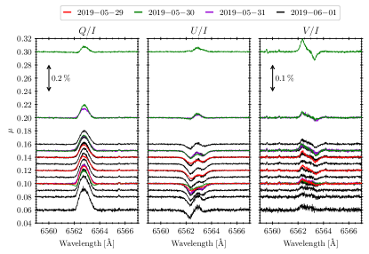
(a)

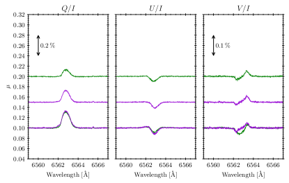
(b)

Figure 1: Center-to-limb variation of the $Q/I$, $U/I$, and $V/I$ profiles of the emergent $\mathrm{H\alpha}\leavevmode\nobreak\$radiation in coronal holes after spatial averaging. Panels (a) and (b) show observations at the North and South limbs, respectively. The vertical axis of the figures shows the $\mu$ position. The vertical row in the $Q/I$ panels indicates the scale of the polarization amplitudes. The noise level, after averaging along the spatial direction of the slit, is about $3\times 10^{-5}$. The reference direction for positive $Q/I$ is the parallel to the nearest limb. The ID of the North limb observations are 01, 02, 03, 05, 06, 07, 08, 23, 24, 25, 28, 29, 30, 31, 32, 33, 34, 35, 36, 37 and 38. The South-limb observations are 09, 10, 26 and 27 (see Table 2).

After averaging all the spatial pixels of the slit covering a region of $0\aas@@fstack{\prime\prime}5\times 200\arcsec$, which correspond to a surface of about 50 Mm² at the disk center, we obtain a single Stokes profile with a noise level lightly above $10^{-5}$. We expect non-zero $Q/I$ signals for an observation near the limb because of the $90^{\circ}$ scattering geometry, as long as the reference direction for $Q>0$ is parallel to the limb. Since the Stokes parameter $U$ does not have any preferred direction, we expect zero $U/I$ signals if the averaged area is large enough to statistically represent the quiet solar atmosphere. The presence of thermal, dynamic and magnetic inhomogeneities will generate non-zero $U/I$ signals. In this subsection we analyze the spatially averaged profiles with the goal of extracting information about the averaged properties of the atmosphere.

Due to the curvature of the solar limb and the $0.5\arcsec$ precision of the limb tracking system, some spatial pixels at the edges of the slit can mix on-disk and off-limb signals, especially for observations very close to the limb. Then, in order to consider spatial pixels fully inside the disk, we select only the pixels that are at least $1\aas@@fstack{\prime\prime}5$ inside the solar disk, which corresponds to pixels at $\mu>0.05$, with $\mu=\cos\theta$ and $\theta$ the heliocentric angle. After removing those pixels, we average the remaining pixels and we obtain one profile for each Stokes parameter at any given limb distance $\mu$.

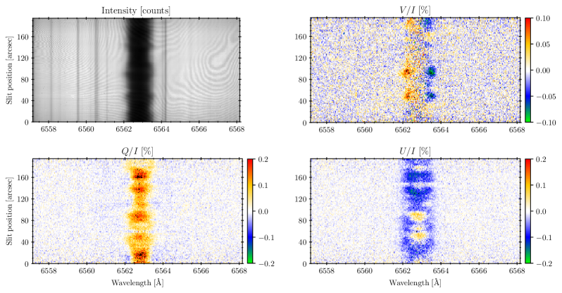
Figure 13: Spectropolarimetric $I$, $V/I$, $Q/I$ and $U/I$ images of th observation with ID 06. The color scale saturates in black at $\pm 0.2\leavevmode\nobreak\ \%$ for $Q/I$ and $U/I$, and $\pm 0.1\leavevmode\nobreak\ \%$ for $V/I$.

Firstly, we analyze the CLV of the linear polarization observed in coronal holes. We took several measurements with the slit parallel to the limb at the North and South poles covering limb distances from $\mu=0.06$ up to $\mu=0.3$. Figure 1 shows the averaged Stokes profiles at different limb distances, from the limb (bottom profile) to the disk center (top profile). Each profile is placed at a position on the vertical axis that corresponds to its $\mu$ value. The different line colors correspond to different observation days (see Table 2). Both, at the North and South limbs, the $Q/I$ profiles are Gaussian-like and their amplitudes decrease with the limb distance. The $U/I$ profiles at the North pole are different from the ones observed at the South pole. The later ones have negative Gaussian-like shapes with similar amplitudes at different $\mu$ values. The profiles at the North limb show two negative lobes, with the blue one larger than the red one, except the ones at $\mu=0.06$ and $0.08$, which present a central positive signal. The three-lobed $U/I$ profiles at the North limb show strong positive bumps at the line-center with negative wings (see Fig. 13). These localized positive bumps are detected in other North-limb observations from different days but not in the observations at the South limb (see 11). Images from the Solar Dynamics Observatory (SDO) do not show any appreciable differences on magnetic activity between both poles, suggesting that these positive bumps in $U/I$ are probably due to localized thermal or dynamic atmospheric conditions. The $V/I$ signals are of the order of $0.02\,\%$ because there is no strong magnetic activity, except at $\mu=0.3$ where the signal is twice as large.

Fig. 2 shows the CLV of the $Q/I$ amplitudes of the profiles in Fig. 1. The North and South limb observations are represented by circles and crosses, respectively. As we saw in Fig. 1, the amplitudes decrease as we approach the disk center. Fig. 2 shows clearly that the amplitudes of the measurements taken on 2019-05-29 (red points, corresponding to the red lines in Fig. 1) are lower than those from 2019-06-01 (black points, corresponding to the black lines in Fig. 1). Fig. 1 shows that the green profile at $\mu=0.1$ has a different shape, with negative wings and a lower line center signal. And in this figure we can clearly see that the amplitude has been reduced by 30% with respect to that of black points. This can be a manifestation of the Hanle effect in the $\mathrm{H\alpha}\leavevmode\nobreak\$line (e.g., Štěpán et al., 2011; Štěpán & Trujillo Bueno, 2011) due to the contribution of the seven fine structure components (see below).

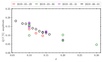
Figure 2: Center-to-limb variation of the $Q/I$ amplitudes of the profiles of Fig. 1. Observations taken at the North and South limbs are indicated by circles and crosses, respectively.

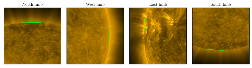
Figure 3: 171 Å SDO intensity images showing the location of the slit of our spectropolarimetric observations (see the green line). The ID of the observations are 01, 09, 12 and 40.

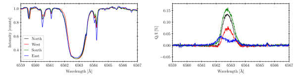
Figure 4: Spatially averaged on-disk observations at $5\arcsec$ inside the limb ($\mu=0.1$) taken in different heliographic limbs. The ID of the observations are: 01, 09, 12 and 40 (see Table 2).

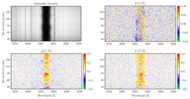
Figure 12: Spectropolarimetric $I$, $V/I$, $Q/I$ and $U/I$ images of th observation with ID 12. The color scale saturates in black at $\pm 0.2\leavevmode\nobreak\ \%$ for $Q/I$ and $UI/$, and $\pm 0.1\leavevmode\nobreak\ \%$ for $V/I$.

It is also interesting to compare spatially averaged $Q/I$ profiles at different solar regions. We consider four observations at $5\arcsec$ ($\mu=0.1$) inside the solar disk. Two observations in the coronal holes at the North and South limbs, one observation at the West limb in a quiet region, and another one in a plage at the East limb. Fig. 3 shows the location of the slit for each observation using SDO images at the 171 Å wavelength. The averaged Stokes profiles at these locations are shown in Fig. 4. The $Q/I$ profiles at the North and South limbs have Gaussian-like shapes with similar amplitudes. At the West limb, the amplitude is twice lower than at the North and South limbs, but the shape remains Gaussian-like. However, the shape of the $Q/I$ profile from the more active East limb is a two-peaked profile, which is similar to the one observed by Gandorfer (2000) but with a more pronounced asymmetry. The lower $Q/I$ amplitude from the quiet West-limb profile can be understood in terms of depolarization by the Hanle effect. In the active East limb, the magnetic field may have larger gradients and may be structured at larger spatial scales than in quiet regions. This may facilitate that the different sensitivity of the overlapping $\mathrm{H\alpha}\leavevmode\nobreak\$transitions to the Hanle effect produce asymmetries in the $Q/I$ core. A physical mechanism leading to the creation of asymmetries in the linear polarization profiles of $\mathrm{H\alpha}\leavevmode\nobreak\$has been proposed by Štěpán & Trujillo Bueno (2010a). For additional developments on the role of magnetic field gradients on the shape of the $\mathrm{H\alpha}\leavevmode\nobreak\$linear polarization profiles, see Štěpán et al. (2011). The spectropolarimetric images of the East limb observation are shown in Fig. 7(b). The other ones can be found in Figs. 10, 11, and 12 of Appendix B.

In addition to the $\mathrm{H\alpha}\leavevmode\nobreak\$line, we have been able to detect faint linear and circular polarization signals in other spectral lines: Ti ii at $6559.56$ Å and Ti i at $6565.50$ Å. $Q/I$ and $V/I$ signals in the Ti ii line are only detected in the regions with strong magnetic fields, where the linear polarization is induced by the Zeeman effect (East limb). We have also detected linear polarization signals in the Ti i line due to scattering with amplitudes of the order of $0.01\,$%, even in regions with strong circular polarization.

3.2 Spatial variation and line shapes

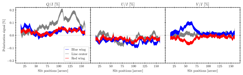
(a)

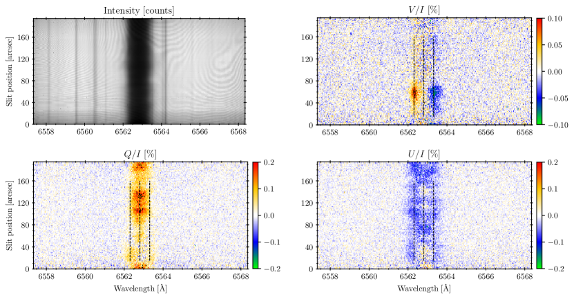
(b)

Figure 5: Panel (a): spatial variation at 3 different wavelengths along a region of the slit of $Q/I$ (left panel), $U/I$ (central panel) and $V/I$ (right panel). The line center wavelength (grey line) is at $\lambda_{0}=6562.81\,$Å. The blue wing (blue line) is at $\lambda_{b}=\lambda_{0}-0.5\,$Å and the red wing (red line) at $\lambda_{r}=\lambda_{0}+0.5\,$Å. The width of the curves indicates the noise level at each spatial pixel. The considered spatial region is shown by the three dashed lines in the panels below. A binning of 2 and 4 pixels along the spatial and spectral dimensions are applied in order to reduce the noise. The spatial resolution of the signals are about $6\arcsec$. Panel (b): spectropolarimetric images. The color scale saturates in black at $\pm 0.2\leavevmode\nobreak\ \%$ for $Q/I$, and $U/I$ and $\pm 0.1\leavevmode\nobreak\ \%$ for $V/I$. Observation taken at the heliospheric North limb, at $\mu=0.14$. The observation ID is 03.

In the previous subsection, we showed how the amplitudes and shapes of the linear polarization spatially averaged profiles change with the limb distance. Such variations allow us to learn about the large-scale structure of the chromosphere at different heights, since the scattering signals of the $\mathrm{H\alpha}\leavevmode\nobreak\$line originate at chromospheric heights Štěpán & Trujillo Bueno (2011). Clearly, small-scale variations are also important in order to decipher how the magnetic and velocity fields change locally.

As we specified in Sect. 2.1, the length of the slit is $200\arcsec$ with a spatial sampling of $1.4\arcsec$. Since the seeing of our observations is not worse than $2\arcsec$, we are limited by the resolution of the CCD, which is twice the spatial sampling (i.e. $\sim 3\arcsec$). This allows us to see relatively small variations on the Stokes profiles along the slit at different regions of the solar disk at the expense of a lower signal-to-noise ratio (SNR). Furthermore, it is important to remember that the integration time of our observations is about 5 to 8 minutes, so that plasma variations can smear or even cancel out the polarization signals (Carlin & Bianda, 2017, and more references therein).

In Fig. 5(a), we show the variation of the polarization signals along the slit from an observation performed in a coronal hole at the North limb, at $\mu=0.14$ with the slit parallel to the limb at three different wavelengths: the line center $\lambda_{0}$ and the near wings at $\lambda_{r,b}=\lambda_{0}\pm 0.5\,$Å. The signals are binned over 2 and 4 spatial and spectral pixels, respectively. Therefore, the spatial resolution is about $6\arcsec$. Figure 5(b) shows the spectropolarimetric images of the same observation to put in context the other figure.

In Fig. 5(a) we can observe several interesting things:

a) The wing signals of the $Q/I$ profiles decrease from $35\arcsec$ to $60\arcsec$, while the $V/I$ amplitudes increase in this region. After this position, the $V/I$ signal decreases until reaching $85\arcsec$ while the $Q/I$ signal wings increase until the $100\arcsec$ slit position. Apparently, the $Q/I$ depolarization in the wings is related to the magnetic fields.

b) The line-core signal of $Q/I$ increases almost linearly from $45\arcsec$ up to $90\arcsec$ along the slit and the $U/I$ signal at the line-center decreases, while the circular polarization signals increase reaching a maximum of $0.1\,\%$ at $60\arcsec$ and then it decreases. The linear polarization at the line core does not seem to be affected by the magnetic fields in this region.

c) It seems that the signal in the wings of $U/I$ remains negative without any significant change in the spatial region where $V/I$ is detected.

d) At $25\arcsec$ slit position, the $Q/I$ signal in the blue wing is twice the signal in the red wing, producing an asymmetric profile. This asymmetry remains visible for $15\arcsec$ along the slit. At these positions, the line-center signal of $U/I$ becomes slightly positive while the wing signals stay negative. At $25\arcsec$ slit position, the $V/I$ signal starts increasing. The asymmetry observed in $Q/I$ is similar to the observed by Gandorfer (2000), although in that case the signal was integrated along a significantly larger spatial region.

e) From $90\arcsec$ slit position to the end, there is no sizable circular polarization. However, we detect two maxima in $Q/I$ at $105\arcsec$ and $130\arcsec$. Near these slit locations, the line-center signal of $U/I$ becomes positive while the blue wing signal slightly decreases. The dynamics of the plasma together with the magnetic field, is capable of modifying the linear polarization signals in a significant way (e.g., Jaume Bestard et al., 2021).

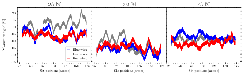
Figure 6: Similar figure to Fig. 5(a), but for another observation at the North limb with ID 06. The spectropolarimetric image of this observation can be found in Fig. 13.

Figure 6 shows the spatial variation of another North-limb observation at $\mu=0.15$, taken during a different day. The $U/I$ signals have 3 positive peaks at the core, at the $50\arcsec$, $65\arcsec$ and $90\arcsec$ positions, keeping a negative signal in the wings. The line-center $Q/I$ signal also presents two peaks at $50\arcsec$ and around $90\arcsec$. The $Q/I$ signals at the wings also increase, but with a slightly larger amplitude in the blue wing of the second peak. These spatial variations of the linear polarization seem to be correlated with the signals detected in $V/I$, reaching amplitudes of $\sim 0.1\%$ at $50\arcsec$ and $95\arcsec$. On the other hand, the $U/I$ signals and the wings of $Q/I$ suddenly vanish at $\sim 150\arcsec$. The $Q/I$ line-center signal does not vanish at this position, but it decreases a factor two with respect to previous and subsequent slit positions, reaching an amplitude of $0.1\%$.

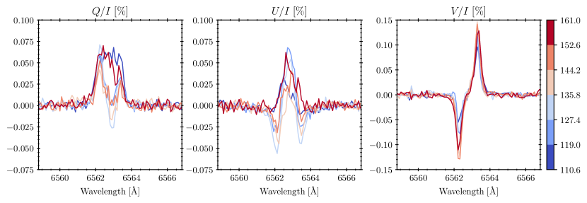
(a)

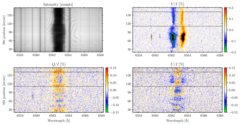
(b)

Figure 7: Panel (a): spatial variation of the $\mathrm{H\alpha}\leavevmode\nobreak\$Stokes profiles shown in Fig. 7(b). We applied a binning of 6 and 10 pixels along the spatial and spectral dimensions, respectively. Each profile, after the spatial binning, covers $8.4\arcsec$ on the slit. The selected region starts at $110.6\arcsec$ and ends at $161\arcsec$ (see the black thin lines in Fig. 7(b)). The ID of the observation used is 40. Panel (b): spectropolarimetric images. The color scale saturates in black at $\pm 0.2\leavevmode\nobreak\ \%$ for $Q/I$, and $U/I$ and $\pm 0.1\leavevmode\nobreak\ \%$ for $V/I$. The black thin lines show the spatial region used in Fig. 7(a). Observation taken at the heliospheric East limb, at $\mu=0.1$. The observation ID is 40.

Figure 7(b) shows similar images but for an observation taken at the East limb. This figure shows the spatial variation of the blue profile of Fig. 4. This observation shows large $V/I$ amplitudes with a maximum at $60\arcsec-80\arcsec$. Along this spatial region of the slit, the linear polarization profiles change several times their sign. This could be an indication of different orientations of the magnetic field. Unfortunately, the spatial resolution is not sufficient for reaching more solid conclusions. However, if we focus on the $Q/I$ signals located between $110\arcsec$ and $160\arcsec$, we see that they become two-peaked profiles with a negative signal in the core. We have an inverted situation in the $U/I$ signals: negative wings with positive signals in the core. In Fig. 7(a) we emphasize the spatial variation within this small region. We have performed a binning of 6 and 10 pixels in the spatial and spectral dimensions, respectively, in order to increase the SNR. The spatial location along the slit is indicated by the color of the profiles, from blue to red. Note that the dark blue linear polarization profile is fully positive and the line core signal is flat, while the $V/I$ profile has the lowest amplitude. As we move along the slit, towards redder profiles, the $Q/I$ line-center signal becomes negative and its profile asymmetric, the wings of the $U/I$ profile become negative and the amplitude of the circular polarization increases, having a maximum at intermediate positions and then it decreases. Interestingly, the reddest $Q/I$ and $U/I$ profiles are similar to the bluest one, while the $V/I$ amplitude is almost twice larger. This spatial variation suggest that the non-symmetric shape of the linear polarization profiles is produced by the magnetic field through the Hanle effect. Note that the averaged blue profile shown in Fig. 4 has this two-peaked shape due to the signals from this region, since outside of it the $Q/I$ signal is practically cancelled out. We want to emphasize that this pattern in the circular and linear polarization signals is detected in other observations (see Fig. 5) and it is almost certainly due to the interplay of the Zeeman and Hanle effects at the different heights of formation of the spectral line wavelengths. While the Zeeman effect is mostly affecting the $V/I$ profile in the deeper atmospheric regions Socas-Navarro & Uitenbroek (2004), the Hanle effect plays a dominant role in the formation of the linear polarization signals in the upper chromosphere (see Fig. 4 of Štěpán & Trujillo Bueno, 2010b).

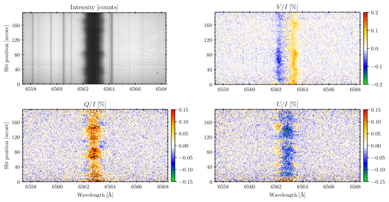
Figure 14: Spectropolarimetric $I$, $V/I$, $Q/I$ and $U/I$ images of th observation with ID 22. The color scale saturates in black at $\pm 0.15\leavevmode\nobreak\ \%$ for $Q/I$ and $UI/$, and $\pm 0.2\leavevmode\nobreak\ \%$ for $V/I$.

The observation shown in Fig. 14 was taken at the same limb, but on 30-05-2019, when the plage region of the East limb was not yet visible. The circular polarization signals indicate the presence of magnetic fields with components parallel to the LOS along the whole slit, without strong variations. On the other hand, the linear polarization signals vary significantly. Note that the wings of the $Q/I$ and $U/I$ profiles also change spatially, something that the previous observations did not show. Furthermore, the sign of both $Q/I$ and $U/I$ profiles seem to be reversed: positive core signals and negative wings in the former, while showing negative core signals and positive wings in $U/I$.

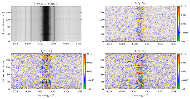
Figure 15: Spectropolarimetric $I$, $V/I$, $Q/I$ and $U/I$ images of th observation with ID 18. The color scale saturates in black at $\pm 0.1\leavevmode\nobreak\ \%$ for $Q/I$, $U/I$ and $V/I$.

The previous images show the Stokes parameters of the $\mathrm{H\alpha}\leavevmode\nobreak\$radiation emerging near the limb, where we expect significant amplitudes due to the scattering geometry. However, Fig. 15 shows an observation taken at $\mu=0.5$ at the West limb (quiet region) with relatively large signals, $\sim 0.1\,\%$, that show an interesting spatial variation along the slit. In this case, the limited spatial resolution and the noise of the signal make it very difficult, nearly impossible, to identify any pattern. Moreover, at our spatial resolution the scattering polarization signals near the disk center are expected to be faint and the current telescopes need large exposure times to gain sufficient SNR.

It is of interest to remark that the high polarimetric sensitivity achieved with ZIMPOL allows us to detect spatial variation of the polarization signals of the Ti ii line at $\lambda=6559.56\,$Å in strongly magnetized regions. In Fig. 7(b), we detect conspicuous Zeeman signals in $Q/I$ and $V/I$. Although the signals are weak, we can distinguish that the circular polarization profiles change their sign at about $100\arcsec$. This means that $B_{||}$ at the formation height of this line changes the sign at this location. Interestingly, the $V/I$ signal of $\mathrm{H\alpha}\leavevmode\nobreak\$does not show any sign change there.

3.3 Net circular polarization

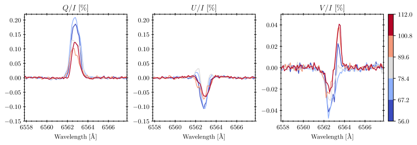
(a)

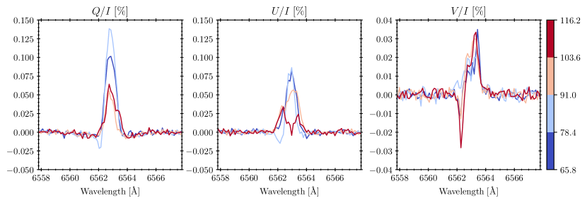
(b)

Figure 8: Panel (a): Stokes profiles at the center of the slit located at $\mu=0.1$. After averaging 8 spatial pixels, each profile covers $11.2\arcsec$ along the slit. The ID of the observation is 09. Panel (b): Stokes profiles at the center of the slit located at $\mu=0.09$. After averaging 9 spatial pixels, each profile covers $12.6\arcsec$ along the slit. The ID of the observation is 11. Spatial variation of the Stokes profiles along the slit for different observations. A binning of 12 pixels in the spectral dimension is applied in both observations.

Net circular polarization (NCP) signals with $V/I$ amplitudes up to $10^{-2}$ in the $\mathrm{H\alpha}\leavevmode\nobreak\$line have been reported in prominences (see López Ariste et al., 2005), although observations carried out by Ramelli et al. (2005) with a different spectropolarimeter (ZIMPOL) could not confirm them. The latter observations could find only NCP of a few times $10^{-4}$, which were considered to be compatible with the alignment to orientation mechanism Landi Degl’Innocenti & Landolfi (2004). Here we report NCP signals in quiet regions near the limb. Observations with ZIMPOL taken near the solar limb have to be considered carefully because the limb tracking precision is limited and the resulting polarization profiles can mix on-disk and off-limb solar disk signals. To avoid this problem, we only selected slit pixels that are located at least $3\arcsec$ inside the solar disk. With this condition, we can assure that the detected polarization signals correspond to on-disk pixels, in spite of possible deviations of the slit position due to occasional bad seeing conditions and the limited limb tracking precision.

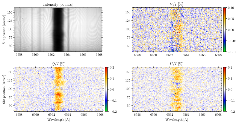
Figure 16: Spectropolarimetric $I$, $V/I$, $Q/I$ and $U/I$ images of th observation with ID 11. The color scale saturates in black at $\pm 0.2\leavevmode\nobreak\ \%$ for $Q/I$ and $UI/$, and $\pm 0.1\leavevmode\nobreak\ \%$ for $V/I$.

Figure 8 shows two observations where NCP is detected, as well as how the amplitudes and shapes change along the slit. In order to improve the SNR, we average 12 spectral pixels, and 8 spatial pixels for the panel (a) and 9 spatial pixels for the panel (b). Actually, the panel (a) shows the same spatially averaged observation of Fig. 4 (green curve; also shown in Fig. 11). In panel (a) we see the reddest $V/I$ profile with an antisymmetric shape, but as we move along the slit (to bluer profiles), the signal becomes fully negative. At the same time, the linear polarization amplitudes increase as the shape of the circular polarization $V/I$ profile becomes a one-lobe profile. At the same time, the wings of the $U/I$ profiles become positive. We see a similar behaviour in panel (b), but with the circular polarization signal fully positive (this observation is also shown in Fig. 16).

3.4 The Weak Field Approximation

The $\mathrm{H\alpha}\leavevmode\nobreak\$line is very broad because the hydrogen is the lightest atom and its Doppler width ($\Delta\lambda_{\mathrm{D}}$) is usually much larger than the Zeeman splitting of the levels ($\Delta\lambda_{B}$). That is one of the necessary conditions for applying the so-called weak field approximation (WFA). The other condition of the WFA validity is that the LOS component of the magnetic field, $B_{||}$, is constant with optical depth. In fact, this is a very strong assumption in the case of the $\mathrm{H\alpha}\leavevmode\nobreak\$line since its formation height spans few thousands of kilometers from the photosphere to the top of the chromosphere. However, the method can provide at least a rough estimate of the magnetic field strength with very little effort. Therefore, we dedicate this section to such quantitative analysis.

A detailed derivation of this approximation can be found in Landi Degl’Innocenti & Landolfi (2004). Under the assumptions mentioned above, the WFA leads to an expression for the Stokes $V$ profile of the form

$$V(\lambda)=-4.6682\times 10^{-13}\,\lambda_{0}^{2}\,\bar{g}_{\mathrm{eff}}\,B_{||}\,\frac{\partial I(\lambda)}{\partial\lambda}\,,$$ (1)

where $\lambda_{0}$ is in Å, $B_{||}$ is the magnetic field component along the LOS and it is in G, and $\bar{g}_{\mathrm{eff}}$ is the effective Landé factor of the $\mathrm{H\alpha}\leavevmode\nobreak\$line which takes the value 1.048 following Casini & Landi Degl’Innocenti (1994). The investigation done by Socas-Navarro & Uitenbroek (2004) calculated the response functions in 1D atmospheric models at $\mu=1$ and found that the $V$ signals are mainly sensitive to photospheric magnetic fields. However, Leenaarts et al. (2012) showed that 1D radiative transfer calculations are not reliable for synthesizing the emergent intensity of this line, and that a 3D treatment is needed to model chromospheric structures (e.g., fibril-like structures) using line-core intensity maps. Nagaraju et al. (2020) applied the WFA to sunspots spectropolarimetric observations in the $\mathrm{H\alpha}\leavevmode\nobreak\$line. It is important to remark that the $\mathrm{H\alpha}\leavevmode\nobreak\$line is the result of seven blended radiative transitions and the applicability of the WFA needs to be carefully investigated. The fact that the synthesized line-core intensity in 3D models traces chromospheric structures does not imply that the retrieved $B_{||}$ through the WFA corresponds to chromospheric heights. In a future theoretical investigation we want to evaluate the reliability of the inferred magnetic fields through the WFA by means of comparing the observations shown here and a detailed 3D radiative transfer modelling. As a first step in this first paper, we apply the WFA to infer and report the estimated magnetic field component along the LOS in different regions of the solar disk with different magnetic activities.

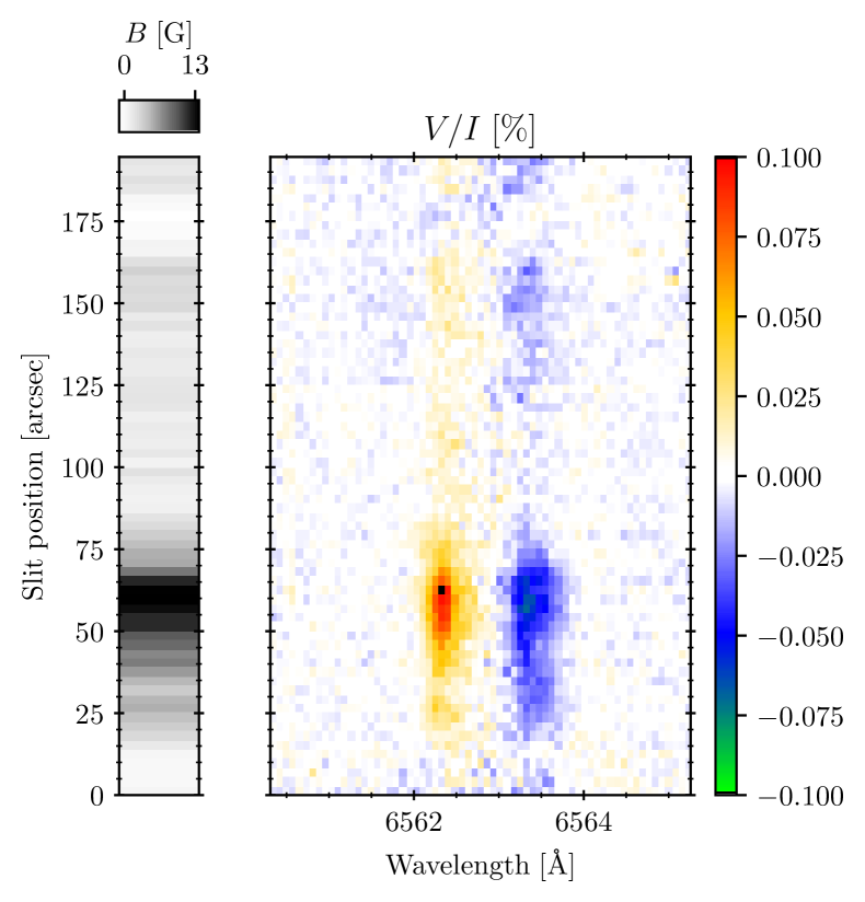
(a)

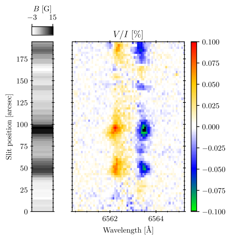
(b)

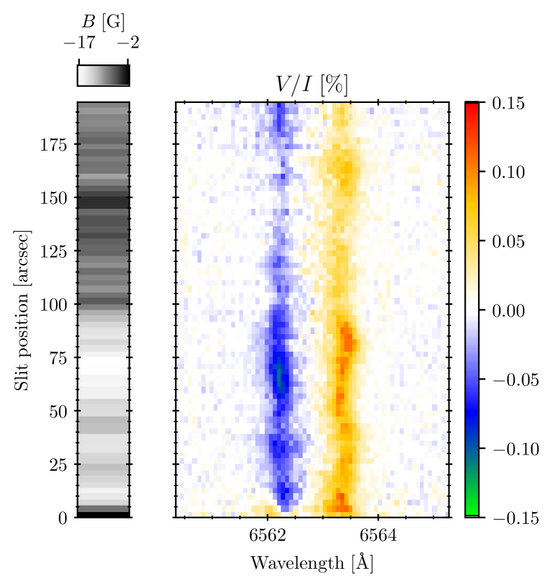
(c)

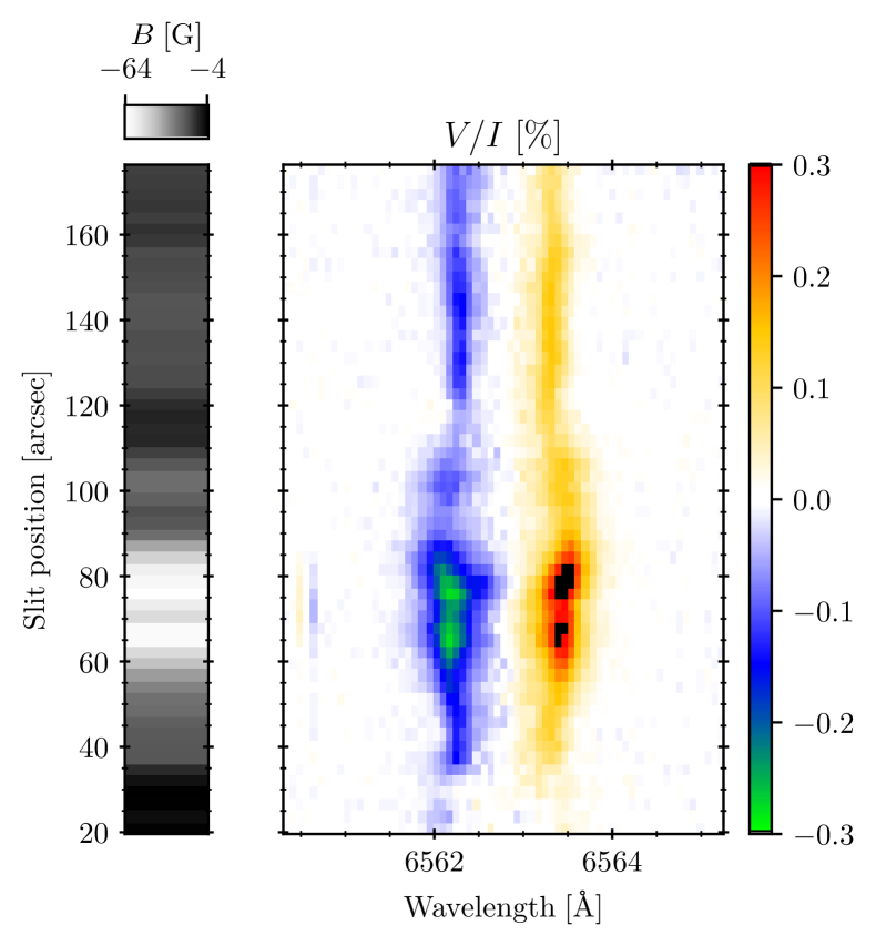
(d)

Figure 9: Panel (a): slit located at North at $\mu=0.14$. Observation ID 03.. Panel (b): slit located at North at $\mu=0.15$. Observation ID 06. Panel (c): slit located at East at $\mu=0.13$. Observation ID 22. Panel (d): slit located at East at $\mu=0.10$. ID 40. Each panel is formed by two subpanels. Left subpanel: retrieved longitudinal component $B_{||}$ of the magnetic field. Right subpanel: the circular polarization signals.

Assuming that the noise of our observations follows a Gaussian distribution, we can apply the equations derived in Martínez González et al. (2012) in order to calculate $B_{||}$. To increase the SNR, we applied a binning of 8 and 2 pixels in the spectral and spatial dimensions, respectively. Moreover, we masked several spectral lines near the $\mathrm{H\alpha}\leavevmode\nobreak\$line that worsened the fit. Such lines and the removed spectral region can be found in Table 1. We have to bear in mind that the spatial resolution is low, and even more after binning. Then, the obtained $B_{||}$ indicates the magnetic flux inside a spatial region of approximately $3\arcsec\times 0.5\arcsec$.

Table 1: Removed spectral lines.

$\lambda_{0}$ [Å]	$\Delta\lambda$ [Å]	Line
6560.57	0.25	Si i
6561.09	0.10	Fe ii
6562.44	0.05	V ii
6563.51	0.15	Co i
6564.15	0.35	Unknown

• Notes. The first and second columns define the spectral region removed before applying the WFA: $\lambda_{0}\pm\Delta\lambda$. We note that $\Delta\lambda$ was set visually, checking the intensity profiles. The third column indicates the element of the transition in case it is known.

If instead of retrieving the magnetic field for spatially averaged profiles we consider the spatial variation of the measured Stokes parameters, we can obtain $B_{||}$ along the slit. Figure 9 shows the obtained $B_{||}$ at each spatial pixel for four observations. The panel (a) and (b) (also shown in Fig. 5(b) and 13) are observations taken at the North limb. At the locations with larger circular polarization signals, with amplitudes of $0.1\,$%, we get $B_{||}\approx 15\,$G, while in regions where the signal is weak but detectable we get magnetic fields of $2-3\,$G. The other two panels, (c) and (d) (shown in Fig. 14 and 7(b)), are observations taken at the East limb. The obtained magnetic field in panel (c) is more or less constant along the slit, reaching a maximum of $18\,$G. On the other hand, we see much stronger circular polarization signals in the panel (d) at some locations, getting $B_{||}\approx 65\,$G. It is important to remember that, as stated above, the obtained values are only estimations of the actual magnetic field and it is not possible to know the error of applying this approximation. The last panel shows an observation taken in a plage region near the limb, and we have to bear in mind that the retrieved magnetic field strengths correspond to the magnetic fields parallel to our LOS. Then, if we make the assumption that the magnetic field permeating the plage is vertical, the $B_{||}$ component is the product of $B$ by $\mu$. Roughly speaking, the retrieved magnetic field along the LOS is one order of magnitude lower than the true magnetic field strength.

4 Conclusions

Motivated by the need to develop new methods to probe the magnetism of the solar chromosphere, we have initiated an observational and theoretical research project aimed at clarifying the diagnostic potential of spectropolarimetry in the hydrogen $\mathrm{H\alpha}\leavevmode\nobreak\$line. In this respect, the $Q/I$ and $U/I$ profiles of this spectral line are of particular interest because they are dominated by scattering processes, and via the Hanle effect the line-center signals are sensitive to the presence of magnetic fields in the upper solar chromosphere (Štěpán & Trujillo Bueno, 2010a). In contrast, the circular polarization signals are dominated by the Zeeman effect, and they probe deeper atmospheric layers.

In this first paper we have presented an overview of our spectropolarimetric observations of close to the limb regions of the solar disk outside sunspots. The observed regions have varying degrees of magnetic activity, and from the application of the WFA to the observed Stokes $I$ and $V$ signals we have estimated the averaged longitudinal field strength over the spatio-temporal resolution element of the observation.

Concerning the scattering polarization signals, we have given particular attention to the CLV curves corresponding to each of the observed regions, since they are of great interest for our future confrontations with the results from radiative transfer modelling in 3D models of the solar atmosphere. A curious finding is that the $U/I$ profiles from the South and North limbs are different, in spite of the fact that our spatial averaging is smearing out all the local variations of the signals, which suggests different physical conditions in the respective coronal holes. The South limb $U/I$ profiles are fully negative, while the North limb ones have negative wings with the line-core close to zero or even positive (see Fig. 1). However, the $Q/I$ profiles from both limbs are practically identical. On the other hand, the amplitudes of the $Q/I$ profiles from both limbs decrease as we approach the disk center (see Fig. 2), getting an amplitude of $0.18\,\%$ at $\mu=0.06$ and of $0.05\,\%$ at $\mu=0.3$. The spatially averaged $Q/I$ signals in Fig. 4 show fingerprints of the presence of magnetic fields via the Hanle effect. The blue curve (corresponding to the more magnetic region, see Fig. 3) has lower amplitude than the others. Moreover, this profile loses the Gaussian shape and becomes a two-peaked profile, being similar to the signal observed by Gandorfer (2000).

We have also analyzed in detail the spatial variation of the Stokes profiles along the direction of the spectrograph’s slit, finding a rich variability in both the linear and circular polarization signals. Such spatial variations are not easy to interpret because the $\mathrm{H\alpha}\leavevmode\nobreak\$line is a multiplet with several overlapped transitions that are formed at slightly different heights in the inhomogeneous plasma of the solar chromosphere. However, we have been able to identify some patterns relating the linear and circular polarization signals, which may be useful for the interpretation of the observations. In most cases, in the presence of significant $V/I$ signals the core of the $Q/I$ profiles are reduced and become a two-peaked profile, or they just loose their Gaussian shape and turn into an asymmetric profile. Some examples can be seen in Fig. 5(b), 7(b) and 13. Štěpán & Trujillo Bueno (2011) performed a 1D radiative transfer investigation of the generation and transfer of the scattering polarization in $\mathrm{H\alpha}\leavevmode\nobreak\$, and concluded that the presence of spatial gradients in the strength of the magnetic field in the upper chromosphere can produce a line-core asymmetry in the $Q/I$ profile, such as that observed by Gandorfer (2000) without spatio-temporal resolution. This possibility could explain the deformation we have observed in the $Q/I$ profile.

Interestingly, in our observations we have detected net circular polarization signals at some positions along the spatial direction of the slit in chromospheric regions. Furthermore, we have been able to detect spatial variations of the linear and circular polarization signals near such locations. In two different observations at different solar limbs, the linear polarization amplitude increases as the circular polarization becomes a one-lobe profile. These variations could put some constraints for deciphering the physical mechanism that creates such NCP signals. The NCP detected in Fig. 11 at $75\arcsec$ is remarkable. Fig. 8(a) shows how the linear polarization amplitude increases as the circular polarization becomes negative. Similar signals are found in Fig. 8(b), which corresponds to the spectropolarimetric images shown in 16. Although the Stokes V signals are still noisy after averaging some pixels and some features cannot be fully trusted, the NCP profiles lie above the noise level and we believe they are real. Given that the densities and temperatures in prominences are similar to those of the upper chromosphere, a theoretical explanation based on the semi-classical impact approximation theory of collisions of hydrogen, protons, and electrons in the presence of magnetic fields could perhaps provide a theoretical explanation of these curious NCP observations (Štěpán & Sahal-Bréchot, 2008). If such a hypothesis is confirmed by close-coupling calculations, it could provide very strong constrains on the plasma density and the magnetic field vector.

The high polarimetric sensitivity of our observations with ZIMPOL at IRSOL has allowed us to detect an extremely rich spatial variability of the scattering polarization of the $\mathrm{H\alpha}\leavevmode\nobreak\$line, in spite of the low spatial resolution of this instrumental setup. This strongly motivates us to continue spectropolarimetric observations of the $\mathrm{H\alpha}\leavevmode\nobreak\$line using the new generation of solar telescopes, namely the Daniel K. Inouye Solar Telescope (DKIST; Rimmele et al., 2020) and the future European Solar Telescope (EST; Collados et al., 2013). Equally important is to theoretically investigate how are the Stokes profiles of the $\mathrm{H\alpha}\leavevmode\nobreak\$line in today’s 3D models of the solar atmosphere, taking into account the joint action of scattering processes and the Hanle and Zeeman effects. This will be the topic of our next paper.

Appendix A Table of observations

Table 2: Information about the observations.

ID	Date (UTC)	Exposure time (s)	$\mu=\cos\theta$	$\sigma_{\mathrm{noise}}[\times 10^{-4}]$	Slit position
01	2019-05-29 - 07:44:23	569	0.10	$1.6$	North
02	2019-05-29 - 08:08:14	569	0.12	$1.8$	North
03	2019-05-29 - 08:18:41	568	0.14	$1.8$	North
04	2019-05-29 - 08:29:42	568	0.00	$2.3$	North
05	2019-05-30 - 07:47:13	569	0.10	$1.6$	North
06	2019-05-30 - 07:58:17	549	0.15	$1.6$	North
07	2019-05-30 - 08:23:39	345	0.20	$2.3$	North
08	2019-05-30 - 08:34:35	324	0.30	$2.3$	North
09	2019-05-30 - 09:20:58	272	0.10	$2.2$	South
10	2019-05-30 - 09:36:21	324	0.20	$2.4$	South
11	2019-05-30 - 15:10:01	344	0.09	$2.3$	West
12	2019-05-30 - 15:16:07	344	0.10	$2.3$	West
13	2019-05-30 - 15:22:12	344	0.11	$2.4$	West
14	2019-05-30 - 15:28:18	344	0.12	$2.4$	West
15	2019-05-30 - 15:35:27	344	0.13	$2.4$	West
16	2019-05-30 - 15:41:41	345	0.14	$2.4$	West
17	2019-05-30 - 15:48:13	345	0.14	$2.4$	West
18	2019-05-30 - 15:57:57	286	0.50	$2.5$	West
19	2019-05-30 - 16:22:28	344	0.10	$2.5$	East
20	2019-05-30 - 16:30:39	344	0.11	$2.6$	East
21	2019-05-30 - 16:37:05	345	0.12	$2.7$	East
22	2019-05-30 - 16:43:21	343	0.13	$2.6$	East
23	2019-05-31 - 09:22:15	344	0.10	$2.2$	North
24	2019-05-31 - 09:30:09	345	0.15	$2.3$	North
25	2019-05-31 - 09:55:03	324	0.20	$2.3$	North
26	2019-05-31 - 10:13:49	344	0.10	$2.6$	South
27	2019-05-31 - 10:21:12	344	0.15	$2.4$	South
28	2019-06-01 - 07:20:21	282	0.06	$2.9$	North
29	2019-06-01 - 07:26:12	282	0.08	$2.7$	North
30	2019-06-01 - 07:31:34	281	0.09	$2.6$	North
31	2019-06-01 - 07:36:58	282	0.10	$2.6$	North
32	2019-06-01 - 07:48:01	282	0.11	$2.6$	North
33	2019-06-01 - 07:53:25	282	0.12	$2.6$	North
34	2019-06-01 - 07:59:35	282	0.13	$2.6$	North
35	2019-06-01 - 08:04:38	281	0.14	$2.5$	North
36	2019-06-01 - 08:16:42	282	0.14	$2.5$	North
37	2019-06-01 - 08:21:51	281	0.15	$2.4$	North
38	2019-06-01 - 08:27:00	282	0.16	$2.4$	North
39	2019-06-02 - 15:39:54	344	0.08	$2.6$	East (plage)
40	2019-06-02 - 15:46:32	344	0.10	$2.6$	East (plage)
41	2019-06-02 - 15:52:57	343	0.12	$2.7$	East (plage)
42	2019-06-02 - 15:59:55	344	0.14	$2.7$	East (plage)
43	2019-06-02 - 16:06:29	344	0.15	$2.6$	East (plage)
44	2019-06-02 - 16:12:52	344	0.16	$2.7$	East (plage)
45	2019-06-02 - 16:21:05	345	0.38	$2.5$	East (faculae)
46	2019-06-02 - 16:29:40	285	0.08	$3.4$	West
47	2019-06-02 - 16:37:40	284	0.10	$3.3$	West

• Notes. First column: identifier of the observation. Second column: date and time of the observation in UTC. Third column: exposure time in seconds for each of the two measurements of each run, $(I,\,Q/I,\,V/I)$ and $(I,\,U/I,\,V/I$). Fourth column: cosine of the heliocentric angle. Fifth column: standard deviations of the noise per pixel in the polarization images. Last column: slit position on the solar disk. The plage at the East limb was not visible until the 31th of May. For this reason, the observations of the 2nd of June has been differentiated from the ones on the 31th of May.

Appendix B Additional figures

Figure 10: Spectropolarimetric $I$, $V/I$, $Q/I$ and $U/I$ images of th observation with ID 01. The color scale saturates in black at $\pm 0.2\leavevmode\nobreak\ \%$ for $Q/I$ and $UI/$, and $\pm 0.1\leavevmode\nobreak\ \%$ for $V/I$.

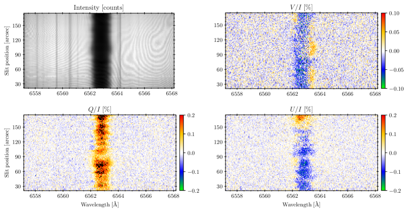
Figure 11: Spectropolarimetric $I$, $V/I$, $Q/I$ and $U/I$ images of th observation with ID 09. The color scale saturates in black at $\pm 0.2\leavevmode\nobreak\ \%$ for $Q/I$ and $UI/$, and $\pm 0.1\leavevmode\nobreak\ \%$ for $V/I$.