Bootstrapping Informative Graph Augmentation via A Meta Learning Approach

Abstract

Recent works explore learning graph representations in a self-supervised manner. In graph contrastive learning, benchmark methods apply various graph augmentation approaches. However, most of the augmentation methods are non-learnable, which causes the issue of generating unbeneficial augmented graphs. Such augmentation may degenerate the representation ability of graph contrastive learning methods. Therefore, we motivate our method to generate augmented graph with a learnable graph augmenter, called MEta Graph Augmentation (MEGA). We then clarify that a ”good” graph augmentation must have uniformity at the instance-level and informativeness at the feature-level. To this end, we propose a novel approach to learning a graph augmenter that can generate an augmentation with uniformity and informativeness. The objective of the graph augmenter is to promote our feature extraction network to learn a more discriminative feature representation, which motivates us to propose a meta-learning paradigm. Empirically, the experiments across multiple benchmark datasets demonstrate that MEGA outperforms the state-of-the-art methods in graph self-supervised learning tasks. Further experimental studies prove the effectiveness of different terms of MEGA. Our codes are available at https://github.com/hang53/MEGA.

1 Introduction

Recently, there has been a surge of interest in learning a graph representation via self-supervised Graph Neural Network (GNN) approaches. GNNs, inheriting the powerful representation capability of neural networks, emerged as benchmark approaches over many graph representation learning tasks. Early works mostly require task-dependent labels to learn a graph representation. However, annotating graphs is a rather challenging task compared to labeling common modalities of data, especially in specialized domains. Therefore, recent research efforts are dedicated to developing self-supervised graph representation learning methods, which can eliminate the dependency of the labels Hu et al. (2020a).

Graph contrastive learning (GCL), one of the most popular self-supervised methods in graph representation learning, is proposed based on GNNs and contrastive learning. Under the learning paradigm of contrastive learning, GCL generates augmented graphs by adopting graph augmentation Hassani and Khasahmadi (2020). After graph encoding, the augmented and original features of the same graph are treated as positives, and the features of different graphs are treated as negatives. The object of GCL is to learn a good graph representation by pulling the positives close and pushing the negatives apart. However, most of the graph augmentation approaches are non-learnable, which causes two issues: 1) the augmentation is excessively weak, e.g., the augmented graph is indistinguishable from the original graph, and the contrastive learning model can hardly mine consistent knowledge from them; 2) the augmentation introduces overmuch noise, and the augmented graph is even more similar to other graphs. The mentioned issues weaken GCL’s ability to learn a discriminative representation. Therefore, we motivate our method to directly learn a graph augmentation, which can assist GCL in generating a good graph representation.

We aim to learn a ”good” graph representation that can have impressive performance on downstream tasks, but what is an exact ”good” representation? From Grill et al. (2020) Ermolov et al. (2021), we notice that, at the instance-level, a good representation naturally has uniformity, e.g., features of different samples are scattered throughout the hidden space instead of collapsing to a point. However, such constraint does not consider the representation’s collapse at the feature-level. For instance, the learned representation has 256 dimensions, but most of them have few differences, which implies that much information learned by the representation is redundant Zbontar et al. (2021). Such redundant information may lead to limited informativeness of the representation and degenerate the representation to model truly discriminative information. Therefore, we motivate our method to learn a ”good” representation with uniformity at the instance-level and informativeness at the feature-level.

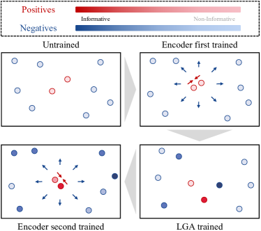
Figure 1: An illustration example of the training process of MEGA. The figure shows the features in hidden space during training. Red points depicts the positive features and blue points depicts the negative features at the instance-level. The gradation of color denotes the informativeness at the feature-level.

To this end, we propose MEta Graph Augmentation (MEGA) to guide the encoder to learn a discriminative and informative graph representation. For training the encoder, we follow the common setting of contrastive learning Chen et al. (2020). The well self-supervised contrastive learning approach leads the features to be scattered in the hidden space. However, in practice, the sufficient self-supervision of the contrastive learning approach demands hard (informative at the instance-level) features of positive and negative samples, e.g., positive features that are relatively far apart and negative features that are relatively close in the hidden space. For instance, Chen et al. (2020) leverages large batch and memory bank to include more hard features, Chuang et al. (2020) explore to emphasize hard features in training. At the instance-level, our motivation is to straightforwardly generate hard graph features by a learnable graph augmenter (LGA), which uses the encoder’s performance in one iteration to generate hard features for the next iteration by updating the graph augmentation. Note that the objective of LGA is not to promote convergence of contrastive loss. On the contrary, we expect LGA to generate an augmented graph that can increase the difficulty of the self-supervision problem (i.e., contrasting). Contrastive learning aims to put the original and augmented features of a graph together and push the features of different graphs away, and LGA aims to degenerate such a process. Therefore, the LGA augmented graph feature must be hard for contrastive learning. To ensure the informativeness of the learned representation at the feature-level, we propose to train LGA to augment the graph so that it can improve the encoder to generate a representation with informativeness at the feature-level. As shown in Figure 1, LGA is like a teacher that shows different hard and informative examples (augmented graphs) to the encoder, and the contrastive loss leads the encoder to learn discriminative knowledge from them.

The reason why we take a meta-learning approach to update LGA is as follows: the learning paradigm of meta-learning ensures that the optimization objective of LGA is improving the encoder to learn representations with uniformity at the instance-level and informativeness at the feature-level from graphs. However, a regular learning paradigm, e.g., directly optimizing LGA by the loss of measuring the uniformity and informativeness of features in hidden space, can only ensure that the features learned from the augmented graph are modified. However, the features learned from the original graph could be collapsed or non-informative. Concretely, the meta-learning paradigm ensures that the encoder learns the knowledge to generate good representations with uniformity at the instance-level and informativeness at the feature-level.

Contributions. The takeaways of this paper are as follows:

• We propose a learnable approach to generate informative graph augmentation, called meta graph augmentation, which boosts the performance of graph contrastive learning.

• We propose an auxiliary meta-learning approach to train the learnable graph augmenter, which guides the encoder to learn a representation with uniformity at the instance-level and informativeness at the feature-level.

• We conduct experiments to compare our method with state-of-the-art graph self-supervised learning approaches on benchmark datasets, and the results prove the superiority of our method.

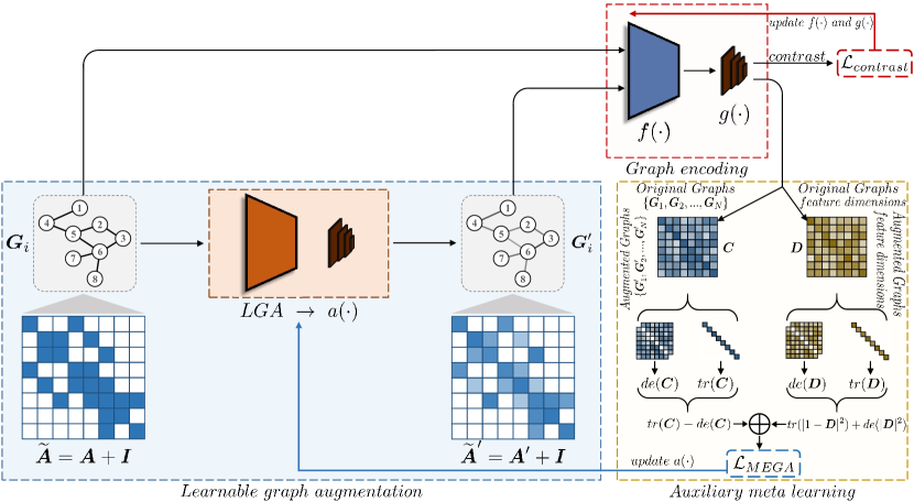
Figure 2: MEGA’s architecture. MEGA uses LGA to generate augmented graph, which and the original graph are encoded together. In one iteration, the encoder and projection head are trained by back-propagating $\mathcal{L}_{contrast}$, and in the next iteration, the LGA is trained by performing the second-derivative technique on $\mathcal{L}_{MEGA}$. The encoder is trained until convergence.

2 Related Works

In this section, we review some representative works on graph neural networks, graph contrastive learning, and meta-learning, which are related to this article.

Graph Neural Networks (GNN).

GNN can learn the low-dimensional representations of graphs by aggregating neighborhood information. These representations can then be applied to various kinds of downstream tasks. Like other neural network structures, GNNs developed many variants. Graph Convolution Networks (GCNs) Kipf and Welling (2016), as an extension of the convolutional neural network on graph-structured data, use convolution operation to transform and aggregate features from a node’s graph neighborhood. Xu et al. (2018) shows that GNNs are at most as powerful as the Weisfeiler-Lehman test in distinguishing graph structures. Based on this idea, Xu et al. (2018) proposed Graph Isomorphism Networks (GINs). Graph Attention Networks (GATs) Veličković et al. (2017) introduces attention mechanisms into graph learning.

Contrastive learning.

Contrastive Learning is a kind of self-supervised learning approach that measures the loss in latent space by contrasting features in hidden space. CMC Tian et al. (2020) uses multi-view data to acquire features for contrasting. In computer vision, many works based on contrastive learning have achieved outstanding results in different kinds of tasks Chen et al. (2020) Zbontar et al. (2021). As in graph learning, contrastive learning also has many applications. For instance, DGI Veličković et al. (2018) learns node representations through contrasting node and graph embeddings. Hassani and Khasahmadi (2020) learns node-level and graph-level representations by contrasting the different structures of a graph.

Meta learning.

The objective of meta-learning is to learn the learning algorithm automatically. Early works Schmidhuber (2014) aim to guide the model (e.g., neural network) to learn prior knowledge about how to learn new knowledge, so that the model can efficiently study new information. Recently, researchers explored using meta-learning to find optimal hyper-parameters and appropriately initialize a neural network for few-shot learning Finn et al. (2017).

3 Methods

In this section, we introduce the proposed MEta Graph Augmentation (MEGA). The architecture of MEGA is depicted in Figure 2. MEGA proposes to learn informative graph augmentation by a meta-learning approach. Guided by the augmented graph, the GNN encoder can mine hidden discriminative knowledge from the original graph.

3.1 Preliminary

We recap necessary preliminary concepts and notations for further exposition. In this paper, we consider attributed graphs $\bm{G}=(\bm{V},\bm{E})$ where $\bm{V}$ is a node set and $\bm{E}$ is the corresponding edge set. For $\bm{G}$, $\{\bm{X_{v}}\in\mathbb{R}^{\bm{V}}|\bm{v}\in\bm{V}\}$ denotes the node attributes.

Learning graph representations.

Given a graph dataset $\mathcal{G}$ including $\bm{G}_{i}$, where $i\in\llbracket{1,N}\rrbracket$. Our objective is to learn an encoder $f(\cdot):\mathcal{G}\to\mathbb{R}^{\bm{D}}$, where $f(\bm{G}_{i})$ is a representation that contains discriminative information of $\bm{G}_{i}$ and can be further used in downstream task. We assume $\bm{G}_{i}$ as a random variable that is sampled i.i.d from distribution $\mathcal{P}\left(\mathcal{G}\right)$ defined over $\mathcal{G}$. To learn such discriminative representation $f(\bm{G}_{i})$, we adopt GNN as the encoder and then perform self-supervised contrastive learning in hidden space.

Graph Neural Networks.

In this paper, we focus on using GNN, message passing GNN in particular, as the encoder $f(\cdot)$. For graph $\bm{G}_{i}=(\bm{V}_{i},\bm{E}_{i})$, we denote $\bm{H}_{\bm{v}}$ as the representation vector, for each node $\bm{v}\in\bm{V}_{i}$. The $k$-th layer GNN can be formulated as:

$${\bm{H}^{(k+1)}_{\bm{v}}}=combine^{(k)}\Big{(}\bm{H}^{k}_{\bm{v}},aggregate^{(k)}(\bm{H}^{k}_{\bm{u}}$$

$$,\forall\bm{u}\in\mathcal{N}(\bm{v}))\Big{)},$$ (1)

where $\mathcal{N}(\bm{v})$ denotes the neighbors of node $\bm{v}$, $\bm{H}^{(k)}$ is the representation vector of the node $\bm{v}$ at layer $k$, and when $k=0$, $\bm{H}^{(0)}$ is initialized with the input node features, which is extracted from $\bm{X}$. $combine$ and $aggregate$ are functions with learnable parameters. After $K$ rounds of massage passing, a readout function will pool the node representations to obtain the graph representation $\bm{h}_{i}$ for $\bm{G}_{i}$:

$${\bm{h}_{i}}=readout\Big{(}\bm{H}_{\bm{v}},\bm{v}\in\bm{V}_{i}\Big{)}.$$ (2)

Contrastive learning.

We follow the preliminaries of contrastive learning Tian et al. (2020): learning an embedding that maximizes agreement between the original and augmented features of the same sample, namely positives, and separates the features of different samples, namely negatives, in latent space. We denote $\bm{G}^{\prime}_{i}$ is the augmented graph of $\bm{G}_{i}$.

To impose contrastive learning, we feed the inputs $\bm{G}_{i}$ and $\bm{G}^{\prime}_{i}$ into the encoder $f(\cdot)$ to learn representations $\bm{h}_{i}$ and $\bm{h}_{i}^{\prime}$, and the representations are further mapped into features $\bm{z}_{i}$ and $\bm{z}_{i}^{\prime}$ by a projection head $g(\cdot)$ Chen et al. (2020). The encoder $f(\cdot)$ and projection head $g(\cdot)$ are trained by contrasting the features, and the loss Oord et al. (2018) is formulated as follows:

$${\mathcal{L}_{contrast}}=-\log\frac{\exp\left(\frac{<\bm{z}^{+}>}{\tau}\right)}{\exp\left(\frac{<\bm{z}^{+}>}{\tau}\right)+\sum{\exp\left(\frac{<\bm{z}^{-}>}{\tau}\right)}}$$ (3)

where $\bm{z}^{+}$ denotes the pair of $\{\bm{z}_{i}^{\prime},\bm{z}_{i}\}$, $\bm{z}^{-}$ is a set of pairs, i.e., $\Big{\{}\{\bm{z}_{j}^{\prime},\bm{z}_{i}\},\{\bm{z}_{i}^{\prime},\bm{z}_{j}\}\Big{|}j\in\llbracket{1,N}\rrbracket,j\neq i\Big{\}}$, $<\cdot>$ denotes a discriminating function to measure the similarity of features, and $\tau$ is the temperature factor Chen et al. (2020). Note that, after training is completed, the projection head $g(\cdot)$ is discarded, and the representations are directly used for downstream tasks.

3.2 Meta Graph Augmentation

Different from benchmark methods that randomly dropping or adding edges to augment a graph Hassani and Khasahmadi (2020) Wan et al. (2020), we motivate our method to impose graph augmentation in an learnable manner Suresh et al. (2021). We rethink the learning paradigm of contrastive learning and find that such an approach relies heavily on hard and informative features in training. Therefore, to boost the performance on downstream tasks of the learned representations, we propose to use a trick of meta-learning to generate informative graph augmentation, which is to guide the encoder to mine discriminative knowledge from graphs.

Learnable graph augmentation.

As the architecture shown in Figure 2, we propose a learnable approach to augment graph. In detail, suppose $\bm{A}$ is the adjacency matrix of $\bm{G}_{i}$ where the initial weights of the connected nodes are set to $1$ and others are valued by $0$. $\widetilde{\bm{A}}=\bm{A}+\bm{I}$, where $\bm{I}$ denotes the self-connection of each node $\bm{e}\in\bm{E}$. We use a neural network $a(\cdot)$, as the LGA (see Appendix for the implementation), to generate the augmented graph $\bm{G}_{i}^{\prime}$ from the original graph $\bm{G}_{i}$, where $\widetilde{\bm{A}}_{i}^{\prime}$ is the adjacency matrix with self-connections $\bm{I}$ of a graph $\bm{G}_{i}^{\prime}$. $\bm{G}_{i}$ and $\bm{G}_{i}^{\prime}$ are then encoded into features $\bm{z}_{i}$ and $\bm{z}_{i}^{\prime}$ by the encoder $f(\cdot)$ and projection head $g{(\cdot)}$.

Method	PROTEINS	MUTAG	DD	COLLAB	RDT-M5K	IMDB-B	IMDB-M
GIN RIU	69.03$\pm 0.33$	87.61$\pm 0.39$	74.22$\pm 0.30$	63.08$\pm 0.10$	27.52$\pm 0.61$	51.86$\pm 0.33$	32.81$\pm 0.57$
InfoGraph	72.57$\pm 0.65$	87.71$\pm 1.77$	75.23$\pm 0.39$	70.35$\pm 0.64$	51.11$\pm 0.55$	71.11$\pm 0.88$	48.66$\pm 0.67$
GraphCL	72.86$\pm 1.01$	88.29$\pm 1.31$	74.70$\pm 0.70$	71.26$\pm 0.55$	53.05$\pm 0.40$	70.80$\pm 0.77$	48.49$\pm 0.63$
AD-GCL	73.46$\pm 0.67$	89.22$\pm 1.38$	74.48$\pm 0.62$	72.90$\pm 0.83$	53.15$\pm 0.78$	71.12$\pm 0.98$	48.56$\pm 0.59$
MEGA-IL	73.89$\pm 0.62$	90.34$\pm 1.20$	75.78$\bf\pm 0.63$	73.54$\pm 0.82$	53.16$\pm 0.65$	71.08$\pm 0.73$	49.09$\pm 0.79$
MEGA	74.20$\bf\pm 0.73$	91.10$\bf\pm 1.34$	75.56$\pm 0.63$	73.96$\bf\pm 0.73$	54.32$\bf\pm 0.79$	71.95$\bf\pm 0.98$	49.52$\bf\pm 0.62$

Table 1: Performance of classification accuracy on datasets from TU Dataset (Averaged accuracy $\pm$ std. over 10 runs). We highlight the best records in bold.

Method	molesol	mollipo	molbbbp	moltox21	molsider
	Regression tasks (RMSE $\downarrow$)		Classification tasks (ROC-AUC % $\uparrow$)
GIN RIU	1.706$\pm 0.180$	1.075$\pm 0.022$	64.48$\pm 2.46$	71.53$\pm 0.74$	62.29$\pm 1.12$
InfoGraph	1.344$\pm 0.178$	1.005$\pm 0.023$	66.33$\pm 2.79$	69.74$\pm 0.57$	60.54$\pm 0.90$
GraphCL	1.272$\pm 0.089$	0.910$\pm 0.016$	68.22$\pm 1.89$	72.40$\pm 1.01$	61.76$\pm 1.11$
AD-GCL	1.270$\pm 0.092$	0.926$\pm 0.037$	68.26$\pm 1.32$	71.08$\pm 0.93$	61.83$\pm 1.14$
MEGA-IL	1.153$\pm 0.103$	0.852$\pm 0.022$	68.34$\pm 1.38$	72.08$\pm 0.82$	63.37$\bf\pm 0.87$
MEGA	1.121$\bf\pm 0.092$	0.831$\bf\pm 0.018$	69.71$\bf\pm 1.56$	72.45$\bf\pm 0.67$	62.92$\pm 0.76$

Table 2: Performance of chemical molecules property prediction in OGB datasets. There are two kinds of tasks, regression tasks and classification tasks. We highlight the best records in bold.

Auxiliary meta-learning.

In contrastive learning, we need hard and informative features to learn discriminative representations. To this end, we build an LGA and train it by a meta-learning approach. In training, we first fix LGA $a_{\sigma}(\cdot)$ and train the encoder $f_{\phi}(\cdot)$ and the projection head $g_{\varphi}(\cdot)$ by back-propagating $\mathcal{L}_{contrast}$, where $\sigma$, $\phi$, and $\varphi$ denote the network parameters of $a(\cdot)$, $f(\cdot)$, and $g(\cdot)$, respectively. Then, $f_{\phi}(\cdot)$ and $g_{\varphi}(\cdot)$ are fixed, and $a_{\sigma}(\cdot)$ is trained by computing its gradients with respect to the performance of $f_{\phi}(\cdot)$ and $g_{\varphi}(\cdot)$, and the meta-learning updating objective is as follows:

$$\mathop{\arg\min}_{\sigma}\bigg{(}\mathcal{L}_{MEGA}\Big{(}g_{\mathring{\varphi}}\big{(}f_{\mathring{\phi}}(\bm{G})\big{)},g_{\mathring{\varphi}}\big{(}f_{\mathring{\phi}}(a_{\sigma}(\bm{G}))\big{)}\Big{)}\bigg{)}$$ (4)

where $g_{\mathring{\varphi}}\big{(}f_{\mathring{\phi}}(\bm{G})\big{)}$ denotes a set of the features extracted from original graphs, $g_{\mathring{\varphi}}\big{(}f_{\mathring{\phi}}(a_{\sigma}(\bm{G}))\big{)}$ denotes a set that includes the features of augmented graphs, and $a_{\sigma}(\bm{G})$ denotes $\bm{G}^{\prime}$. $\mathring{\phi}$ and $\mathring{\varphi}$ represent the corresponding parameters of the encoder and projection head, which are updated with one gradient back-propagation using the contrastive loss defined in Equation 3:

$$\mathring{\phi}=\phi-\ell\nabla_{\phi}\bigg{(}\mathcal{L}_{contrast}\Big{(}g_{\varphi}\big{(}f_{\phi}(\bm{G})\big{)},g_{\varphi}\big{(}f_{\phi}(\bm{G}^{\prime})\big{)}\Big{)}\bigg{)}$$ (5)

$$\mathring{\varphi}=\varphi-\ell\nabla_{\varphi}\bigg{(}\mathcal{L}_{contrast}\Big{(}g_{\varphi}\big{(}f_{\phi}(\bm{G})\big{)},g_{\varphi}\big{(}f_{\phi}(\bm{G}^{\prime})\big{)}\Big{)}\bigg{)}$$

where $\ell$ is the learning rate shared between $\phi$ and $\varphi$. The idea behind the meta updating objective is that we perform the second-derivative trick Liu et al. (2019) to train $a_{\sigma}(\cdot)$. Specifically, a derivative over the derivative (i.e., a Hessian matrix) of $\{\phi,\varphi\}$ is used to update $\sigma$. We compute the derivative with respect to $\sigma$ by using a retained computational graph of $\{\phi,\varphi\}$. Then, $\sigma$ is updated by

$$\sigma=\sigma-\ell^{\prime}\nabla_{\sigma}\bigg{(}\mathcal{L}_{MEGA}\Big{(}g_{\mathring{\varphi}}\big{(}f_{\mathring{\phi}}(\bm{G})\big{)},g_{\mathring{\varphi}}\big{(}f_{\mathring{\phi}}(\widehat{\bm{G}^{\prime}})\big{)}\Big{)}\bigg{)}$$ (6)

where $\ell^{\prime}$ represents the learning rate of $\sigma$, and $\widehat{\bm{G}^{\prime}}$ is the augmented graphs with stop-gradient, which is defined as $\widehat{\bm{G}^{\prime}}=a_{\sigma}(\bm{G}).detach()$. $\mathcal{L}_{MEGA}$ is to train $a_{\sigma}(\cdot)$ to generate hard and informative augmented graphs defined as follows:

$$\mathcal{L}_{MEGA}=\underbrace{tr(\bm{C})-de(\bm{C})}_{instance\ term}+\lambda\underbrace{\left(tr(|\mathbb{1}-\bm{D}|^{2})+de(|\bm{D}|^{2})\right)}_{feature\ term}$$ (7)

where $tr(\cdot)$ denotes the matrix trace function, which is defined as $tr(M)=\sum_{i}M_{ii}$, and $de(\cdot)$ is a matrix calculation function defined as $de(M)=\sum_{i}\sum_{j\neq i}M_{ij}$. $|\cdot|^{2}$ presents a matrix element-wise square function defined as $|M|^{2}=M\times M$ by Hadamard product, and $\mathbb{1}$ presents an identity matrix. $\lambda$ is the coefficient that controls the balance between two terms of $\mathcal{L}_{MEGA}$. Intuitively, the $instance\ term$ aims to lead MEGA to generate instance-level challenging examples for self-supervised learning. Inspired by Zbontar et al. (2021), we design the $feature\ term$ to promote the model to learn dimensionally non-redundant representations, respectively. Concretely, minimizing the proposed $\mathcal{L}_{MEGA}$ by using the second-derivative technique can guide $a_{\sigma}(\cdot)$ to generate hard and informative augmented graphs. $\bm{C}$ denotes the cross-correlation matrix computed between the features of the original graphs and augmented graphs in a batch, as follows:

$$\bm{C}_{ij}=\frac{\bm{z}_{i}\cdot\bm{z}_{j}^{\prime}}{|\bm{z}_{i}|\cdot|\bm{z}^{\prime}_{j}|}$$ (8)

where $i,j\in\llbracket{1,N}\rrbracket$ in a batch $N$ of graphs. $\bm{D}$ is the cross-correlation matrix computed between the multi-dimensional features of the original graphs and the corresponding augmented graphs along the batch, which is defined as:

$$\bm{D}_{pq}=\frac{\sum_{i}(\bm{z}_{i,p}\cdot\bm{z}_{i,q}^{\prime})}{\sqrt{\sum_{i}(\bm{z}_{i,p})^{2}}\cdot\sqrt{\sum_{i}(\bm{z}^{\prime}_{i,q})^{2}}}$$ (9)

where $i\in\llbracket{1,N}\rrbracket$ indexes batch graphs and $p,q\in\llbracket{1,N^{D}}\rrbracket$ index the feature dimension of the original graph and the corresponding augmented graph, and $N^{D}$ denotes the number of feature dimension. $\bm{C}$, $\bm{D}$ aim to train $a_{\sigma}(\cdot)$ to generate hard and informative augmented graphs, respectively. Concretely, the objective of auxiliary meta-learning is to enable LGA to learn augmented graphs that are hard and informative for the encoder, thereby improving the encoder’s learning process for the next iteration.

4 Experiments

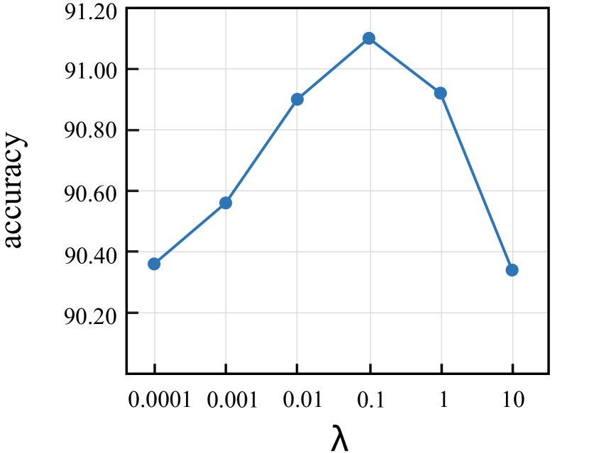
(a) MUTAG

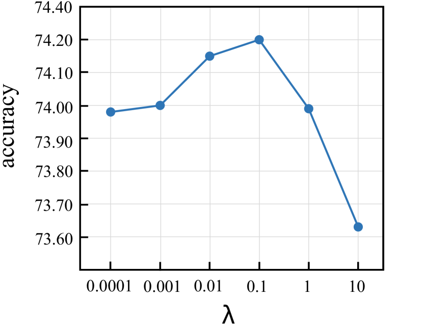
(b) PROTEINS

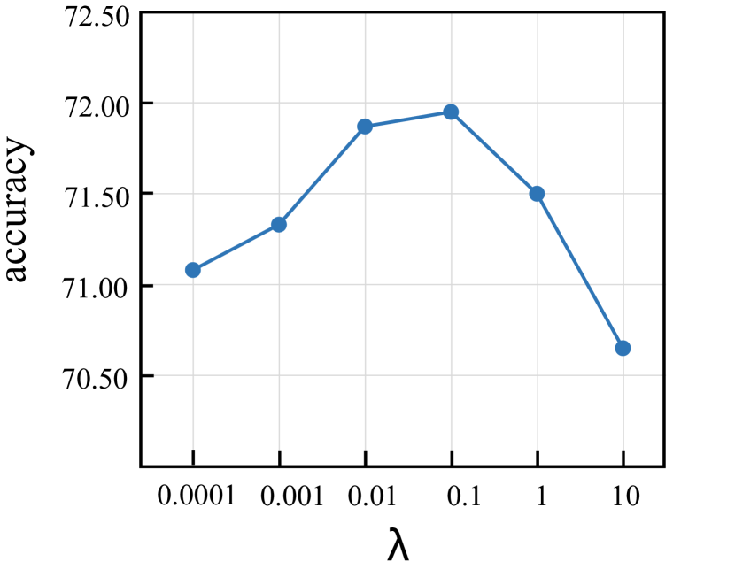
(c) IMDB-B

Figure 3: Results of MEGA’s performance with a range of factor $\lambda$. We perform MEGA on three benchmark datasets: MUTAG, PROTEINS, and IMDB-B. The abscissa axis represents the value of $\lambda$, and the ordinate axis represents the accuracies.

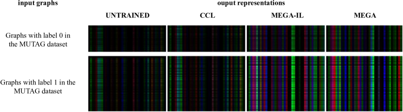
Figure 4: This figure shows the visualized output graph features on the MUTAG dataset. The graph features are projected into a color image in RGB format, where different colors represent different types of features. The abscissa axis represents the output feature dimensions of compared methods, and the ordinate axis represents graphs of different classes.

In this section, we demonstrate the effectiveness of MEGA on various benchmark datasets. Our experiments were conducted in an unsupervised learning setting.

4.1 Comparison with State-of-the-art Methods

Datasets. We evaluate our method on twelve benchmark datasets in two major categories: 1) Social Networks: RDT-M5K, IMDB-B, IMDB-M from TU Dataset Morris et al. . 2) Molecules: PROTEINS, MUTAG, COLLAB and DD from TU Dataset Morris et al. and molesol, mollipo, molbbbp, moltox21 and molsider from Open Graph Benchmark (OGB) Hu et al. (2020b).

Experiment settings.

We compared MEGA with four unsupervised/self-supervised learning baselines, which include randomly initialized untrained GIN (GIN RIU) Xu et al. (2018), InfoGraph Sun et al. (2020), GraphCL You et al. (2020) and AD-GCL Suresh et al. (2021). Experiment results of InfoGraph Sun et al. (2020) and GraphCL You et al. (2020) show that they generally outperform graph kernel and network embedding methods including Kriege et al. (2020), Grover and Leskovec (2016), and Adhikari et al. (2018). As discussed in the method section, the instance-level constrains and feature-level constraints of $\mathcal{L}_{MEGA}$ are balanced by parameter $\lambda$. To study the effects of these constraints, we set $\lambda=0$ for the ablation study, termed MEGA-IL. We followed the experimental protocol of AD-GCL, including the train/validation/test splits. The average classification accuracy with standard deviation on the test results over the last ten runs of training is reported. For a fair comparison, we adopted GIN as the encoder as other baselines do. We adopt the Adam optimizer with a learning rate of $10^{-4}$ for learnable graph augmentation and a learning rate of $10^{-3}$ for graph encoding. We use 50 training epochs on all datasets. All methods adopt a downstream linear classifier or regressor with the same hyper-parameters.

Results.

The results are reported in Table 1 and 2. The results show that MEGA achieves the best results compared with baselines across benchmark datasets. We attribute such performance to MEGA’s abilities to generate both hard and informative augmented graph features. The results show that MEGA outperforms MEGA-IL across most datasets, which proves that the feature-level constraints do improve the network to learn informative representations. MEGA-IL still performs better than most of the baselines that adopt the same encoder and contrastive learning pattern, which means that the instance-level constrains of $\mathcal{L}_{MEGA}$ work well.

4.2 Evaluation of Feature-level Constrains

For further evaluation of feature-level constraints, we change the value of $\lambda$ and observe how the performance changes. We adopt three different datasets, including two molecule datasets and one social network dataset.

The results are reported in Figure 3. The performance changes as the factor $\lambda$ changes. When $\lambda$ takes 0.1, the performance is optimal among all tasks. The results prove that feature-level constraints can enhance the discrimination of features to a certain extent. The feature-level constraints ensure that the generated augmented graph correlates with the original graph, preventing LGA from learning outrageous graph augmentation. However, if we overly increase the impact of feature-level constraints, the generation of hard augmented graph features could be interfered.

4.3 Analyze on Representations

To better understand the quality of the representations learned by MEGA, we visualize the output graph features. For comparison, we conducted experiments on four different networks: (1) UNTRAINED, a randomly initialized GIN encoder without training. (2) CCL, a conventional graph contrastive learning network without our proposed LGA. (3) MEGA-IL, MEGA without feature-level constraints. (4) MEGA.

The results are shown in Figure 4. We intuitively observe the representations of each graph and find that MEGA and MEGA-IL output more ”colorful” results than RI-GIN and CCL, which indicates that their output is more informative. In detail, for MEGA and MEGA-IL, there are many vertical lines of different colors, which means that the difference between the dimensions of the feature is significant. This phenomenon is more evident on MEGA, indicating that the feature-level constraints make the feature dimensions less redundant.

5 Conclusions

This paper proposed a novel meta graph augmentation to boost the representation ability of graph contrastive learning. We apply secondary derivative technique to update a learnable graph augmenter, which is to generate hard and informative augmented graph for contrastive learning. This way, we can yield a representation with uniformity at the instance-level and informativeness at the feature-level.

References

- Adhikari et al. [2018] Bijaya Adhikari, Yao Zhang, Naren Ramakrishnan, and B Aditya Prakash. Sub2vec: Feature learning for subgraphs. In Pacific-Asia Conference on Knowledge Discovery and Data Mining, 2018.
- Chen et al. [2020] Ting Chen, Simon Kornblith, Mohammad Norouzi, and Geoffrey Hinton. A simple framework for contrastive learning of visual representations. In International conference on machine learning. PMLR, 2020.
- Chuang et al. [2020] Ching-Yao Chuang, Joshua Robinson, Lin Yen-Chen, Antonio Torralba, and Stefanie Jegelka. Debiased contrastive learning. arXiv preprint arXiv:2007.00224, 2020.
- Ermolov et al. [2021] Aleksandr Ermolov, Aliaksandr Siarohin, Enver Sangineto, and Nicu Sebe. Whitening for self-supervised representation learning. In International Conference on Machine Learning, pages 3015–3024. PMLR, 2021.
- Finn et al. [2017] Chelsea Finn, Pieter Abbeel, and Sergey Levine. Model-agnostic meta-learning for fast adaptation of deep networks. In Proceedings of the 34th ICML. PMLR, 2017.
- Grill et al. [2020] Jean-Bastien Grill, Florian Strub, Florent Altché, Corentin Tallec, Pierre Richemond, Elena Buchatskaya, Carl Doersch, Bernardo Avila Pires, Zhaohan Guo, Mohammad Gheshlaghi Azar, et al. Bootstrap your own latent-a new approach to self-supervised learning. Advances in Neural Information Processing Systems, 33:21271–21284, 2020.
- Grover and Leskovec [2016] Aditya Grover and Jure Leskovec. node2vec: Scalable feature learning for networks. In Proceedings of the 22nd ACM SIGKDD international conference on Knowledge discovery and data mining, pages 855–864, 2016.
- Hassani and Khasahmadi [2020] Kaveh Hassani and Amir Hosein Khasahmadi. Contrastive multi-view representation learning on graphs. In International Conference on Machine Learning, pages 4116–4126. PMLR, 2020.
- Hu et al. [2020a] W Hu, B Liu, J Gomes, M Zitnik, P Liang, V Pande, and J Leskovec. Strategies for pre-training graph neural networks. In International Conference on Learning Representations (ICLR), 2020.
- Hu et al. [2020b] Weihua Hu, Matthias Fey, Marinka Zitnik, Yuxiao Dong, Hongyu Ren, Bowen Liu, Michele Catasta, and Jure Leskovec. Open graph benchmark: Datasets for machine learning on graphs. Neural Information Processing Systems (NeurIPS), 2020.
- Kipf and Welling [2016] Thomas N Kipf and Max Welling. Semi-supervised classification with graph convolutional networks. arXiv preprint arXiv:1609.02907, 2016.
- Kriege et al. [2020] Nils M Kriege, Fredrik D Johansson, and Christopher Morris. A survey on graph kernels. Applied Network Science, 5(1):1–42, 2020.
- Liu et al. [2019] Shikun Liu, Andrew Davison, and Edward Johns. Self-supervised generalisation with meta auxiliary learning. Advances in Neural Information Processing Systems, 32, 2019.
- [14] Christopher Morris, Nils M Kriege, Franka Bause, Kristian Kersting, Petra Mutzel, and Marion Neumann. Tudataset: A collection of benchmark datasets for learning with graphs. In ICML 2020 Workshop on Graph Representation Learning and Beyond.
- Oord et al. [2018] Aaron van den Oord, Yazhe Li, and Oriol Vinyals. Representation learning with contrastive predictive coding. arXiv preprint arXiv:1807.03748, 2018.
- Schmidhuber [2014] Jürgen Schmidhuber. Learning complex, extended sequences using the principle of history compression. Neural Computation, 4(2):234–242, 2014.
- Sun et al. [2020] Fan-Yun Sun, Jordon Hoffman, Vikas Verma, and Jian Tang. Infograph: Unsupervised and semi-supervised graph-level representation learning via mutual information maximization. In International Conference on Learning Representations, 2020.
- Suresh et al. [2021] Susheel Suresh, Pan Li, Cong Hao, and Jennifer Neville. Adversarial graph augmentation to improve graph contrastive learning. Advances in Neural Information Processing Systems, 34, 2021.
- Tian et al. [2020] Yonglong Tian, Dilip Krishnan, and Phillip Isola. Contrastive multiview coding. In Computer Vision–ECCV 2020: 16th European Conference, Glasgow, UK, August 23–28, 2020, Proceedings, Part XI 16, pages 776–794. Springer, 2020.
- Veličković et al. [2017] Petar Veličković, Guillem Cucurull, Arantxa Casanova, Adriana Romero, Pietro Lio, and Yoshua Bengio. Graph attention networks. arXiv preprint arXiv:1710.10903, 2017.
- Veličković et al. [2018] Petar Veličković, William Fedus, William L Hamilton, Pietro Liò, Yoshua Bengio, and R Devon Hjelm. Deep graph infomax. arXiv preprint arXiv:1809.10341, 2018.
- Wan et al. [2020] Sheng Wan, Shirui Pan, Jian Yang, and Chen Gong. Contrastive and generative graph convolutional networks for graph-based semi-supervised learning. arXiv preprint arXiv:2009.07111, 2020.
- Xu et al. [2018] Keyulu Xu, Weihua Hu, Jure Leskovec, and Stefanie Jegelka. How powerful are graph neural networks? In International Conference on Learning Representations, 2018.
- You et al. [2020] Yuning You, Tianlong Chen, Yongduo Sui, Ting Chen, Zhangyang Wang, and Yang Shen. Graph contrastive learning with augmentations. Advances in Neural Information Processing Systems, 33:5812–5823, 2020.
- Zbontar et al. [2021] Jure Zbontar, Li Jing, Ishan Misra, Yann LeCun, and Stéphane Deny. Barlow twins: Self-supervised learning via redundancy reduction. In International Conference on Machine Learning, pages 12310–12320. PMLR, 2021.