OmniUV: A Multi-Purpose Simulation Toolkit for VLBI Observation

Abstract

We present OmniUV, a multi-purpose simulation toolkit for space and ground VLBI observations. It supports various kinds of VLBI stations, including Earth (ground) fixed, Earth orbit, Lunar fixed, Lunar orbit, Moon-Earth and Earth-Sun Lagrange 1 and 2 points, etc. The main functionalities of this toolkit are: (1) Trajectory calculation; (2) Baseline $uv$ calculation, by taking the availability of each station into account; (3) Visibility simulation for the given $uv$ distribution, source structure and system noise; (4) Image and beam reconstruction. Two scenarios, namely the space VLBI network and the wide field array, are presented as the application of the toolkit at completely different scales. OmniUV is the acronym of “Omnipotent UV”. We hope it could work as a general framework, in which various kinds of stations could be easily incorporated and the functionalities could be further extended. The toolkit has been made publicly available.

1 Introduction

Data simulations are important for the schedule and evaluation of radio interferometric observations (Lanman et al., 2019). RIME (Radio Interferometry Measurement Equation), formulated by Hamaker et al. (1996), provides the basic mathematical framework that links the observed source with the finally recorded signal. Various propagation effects, e.g., phase delays, parallactic angle rotations, receiver gains, beam patterns, could be incorporated into the framework in an elegant and elaborate way (Smirnov, 2011). Since its emergence, most of simulation and calibration tools are developed under this framework: OSKAR (Dulwich et al., 2009) is an interferometer and beam forming simulator package dedicated to the simulation of SKA (Square Kilometer Array, Dewdney et al., 2009). It implements a hierarchical structure, in which both of the antenna field pattern within a station and the station beam are carefully modeled. The use of GPU (Graphics Processing Unit) makes it possible to support the large number of pixels and stations which are required by SKA simulation. pyuvsim (Lanman et al., 2019) is another visibility simulation package with an emphasis on accuracy and design clarity over efficiency and speed, so as to achieve the necessary high level precision for neutral hydrogen studies. It runs on CPU clusters and uses MPI (Message Passing Interface) for parallelization. Besides pyuvsim, the “Radio Astronomy Software Group” also maintains pyuvdata and pyradiosky, which are indispensable for radio interferometry simulations. CASA (the Common Astronomy Software Applications package, Jaeger, 2008) is the primary data processing software for ALMA (the Atacama Large Millimeter/sub-millimeter Array) and VLA (Very Large Array). It also provides tools for visibility simulation based on RIME. CASA is build upon a set of C++ libraries (“CasaCore”) and use Python for its interface, which guarantee both efficiency and user-friendliness. Another tool worth mentioning is MeqTrees (Noordam & Smirnov, 2010). It is designed to be able “to implement an arbitrary measurement equation and to solve for arbitrary sets of its parameters”. To achieve that, a Python-based Tree Definition Language (TDL) is designed and realized. Based on MeqTrees, a new package, MeqSilhouette (Blecher et al., 2017) was developed. It is specifically designed for the accurate simulation of the EHT (Event Horizon Telescope, Akiyama et al., 2019) observation. Based on that, a series of signal corruptions that are important in millimeter wavelength, including troposphere, ISM (Interstellar medium) scattering, and time-variable antenna pointing errors, are taken into account.

All tools mentioned above are intended for ground based telescopes. In principle, if baseline $uv$s are available, those tools could be used for space VLBI simulations as well. However, space VLBI involves calculation of many kinds of trajectories. E.g., Earth orbit, Lunar orbit, Lagrange points, etc. Although all the necessary methods and equations for those calculations are described in the standard textbooks, and all the required ephemeris are publicly available, the actual implementation is still not a trivial task. Moreover, visibility simulation requires not only trajectories, but also the availability of each telescope. For ground based telescopes, availability is mainly determined by the minimum elevation angle. For space telescopes, it also involves the the minimum separation angle between the source and the celestial object being considered. Simulations of space VLBI observations are still in its preliminary stage. Andrianov et al. (2021) demonstrated the improvement of image resolution for the joint observations with Millimetron (Kardashev et al., 2014) and EHT. Palumbo et al. (2019) investigated the possibility of detection for the black hole rapid time variability by expanding the array to include telescopes in LEO (Low Earth Orbit). Also note that the “Fakerat” software package provides support for observation planning, $uv$ calculation and beam/image reconstruction of the RadioAstron mission. However, it is dedicated to that mission only and requires the satellite orbit as input. According to our investigation, at present, no general purpose simulation tools are publicly available for space VLBI observations.

Several space VLBI projects are planned or already under development. China is planning its first Moon-Earth space VLBI experiment in the Chang’E 7 mission. This is based on the 4.2 meter relaying antenna and will perform VLBI observations in X-band. The lunar surface radio telescope is also at discussion. At present, SHAO (Shanghai Astronomical Observatory, Chinese Academy of Sciences) is proposing the Space Low Frequency Radio Observatory, of which two satellites each equipped with a 30 meter radio telescope will be sent to the Earth elliptical orbit (orbit height 2,000 km $\times$ 90,000 km). For the next stage of the Event Horizon Telescope, a very natural extension is to include space radio telescopes, so as to achieve even higher angular resolution. All of those projects require appropriate tools for the simulation of the corresponding VLBI observations.

Keeping this in mind, we develop OmniUV(Liu, 2022), so as to fulfill the requirement of various kinds of VLBI observations. At present, OmniUV provides the following functionalities:

• Trajectory calculation for various kinds of stations;

• $uvw$ and telescope/baseline availability calculation;

• Visibility simulation based on the given source structure and $uvw$, by taking the influence of system noise into account;

• Image and beam pattern reconstruction, so as to provide appropriate tools for the evaluation of observation quality with given configuration.

One thing we want to point out is, for visibility simulation and radio imaging, OmniUV implements both FFT (Fast Fourier Transform) and DFT (Discreate Fourier Transform) methods. The latter one makes it possible to support the $w$ term. For wide field imaging, the variation of phase caused by $w$ term must be taken into account, so as to avoid the distortion of the resulting wide field image. Moreover, FFT method requires gridding, which might introduce errors that are significant for the data processing of 21 cm experiments (Trott et al., 2012). In this work, we will demonstrate the simulation results for configurations of both space VLBI network and wide field array.

This paper is organized as follows: Sec. 2 describes the detailed implementation of the toolkit, including trajectory calculation, $uv$ calculation, visibility simulation and image reconstruction; Sec. 3 demonstrates the application of OmniUV in two typical observation scenarios; Sec. 4 discusses possible future work; Sec. 5 presents the summary.

2 Implementation

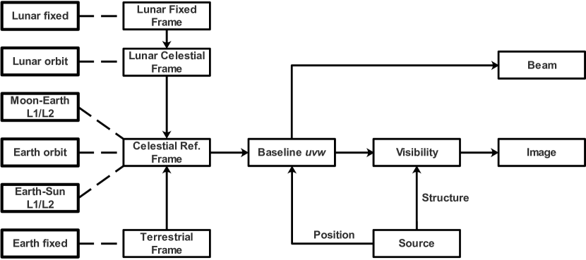
Figure 1: Data flow of the OmniUV toolkit.

Fig. 1 demonstrates the data flow of the OmniUV toolkit. At present, 8 types of stations are supported. For the given trajectory, baseline $uvw$ is calculated. In this process the availability of each telescope is taken into account. Visibilities are calculated for each $uvw$ sampling point. The radio image is constructed accordingly.

2.1 Trajectory calculation

Trajectory calculation involves a series of coordinate transformations. Positions of all kinds of stations are unified in the same frame: the Celestial Reference Frame (CRF). The availability of each station is determined by the angular distances between the source and the celestial objects (Earth, Moon, Sun, etc.). For the Earth/Moon fixed stations, elevation angles are considered as well. In OmniUV, the minimum distance for each object and the minimum elevation angle can be configured explicitly.

2.1.1 Moon stations

OmniUV utilizes the JPL Planetary Ephemeris (version DE-421) Lunar PCKs, which provides the orientation of the Lunar Principal Axis (PA). The Euler angles at the given solar system barycenter Julian date (TDB) are loaded, so as to build the rotation matrices for the conversion from LFF (Lunar Fixed Frame) to LCF (Lunar Celestial Frame). The relative position of the Moon to the Earth is retrieved from the JPL Planetary Ephemeris (version DE-421) SPK. In this way the coordinates of the Moon fixed and the orbit stations in CRF are calculated.

2.1.2 Earth stations

The trajectories of the Earth orbit stations are described with 6 orbital elements and are calculated in CRF. The trajectory calculation of the Earth fixed stations involves translation from TF (Terrestrial Frame) to CRF, which requires the matrices of polar motion (wobble, $\mathbf{W}$), Earth rotation ($\mathbf{R}$), precession and nutation ($\mathbf{PN}$). These calculations require the EOP (Earth Orientation Parameter), which are updated on a daily basis. Since the retrieve of the EOP might not be a trivial task for some users, the input of the EOP is optional. It is the decision of the user to provide EOPs at specific dates to achieve the necessary precision of the trajectory calculation.

2.1.3 Stations at Lagrange points

The location of the L1 point is the solution to the following equation:

$$\frac{M_{1}}{(R-r)^{2}}=\frac{M_{2}}{r^{2}}+\left(\frac{M_{1}}{M_{1}+M_{2}}R-r\right)\frac{M_{1}+M_{2}}{R^{3}},$$ (1)

where $r$ is the distance of the L1 point to the smaller object, $R$ is the distance between the two objects, $M_{1}$ and $M_{2}$ are the masses of the large and the small object, respectively. Given $R$, $M_{1}$ and $M_{2}$, $r$ could be solved numerically.

The location of the L2 point is the solution to the following equation:

$$\frac{M_{1}}{(R+r)^{2}}+\frac{M_{2}}{r^{2}}=\left(\frac{M_{1}}{M_{1}+M_{2}}R+r\right)\frac{M_{1}+M_{2}}{R^{3}},$$ (2)

with parameters defined as that in Eq. 1.

The relative positions of the Moon and the Sun to the Earth are retrieved from the JPL Planetary Ephemeris (version DE-421). Noting that the L1/L2 points lie on the line defined by the two celestial objects, their positions could be derived with the corresponding $r$, as listed in Tab. 1.

Table 1: The L1/L2 $r$ values of the Moon-Earth and the Earth-Sun system. $r$ is given in unit of $R$ (distance between the two celestial objects).

	Moon-Earth		Earth-Sun
	L1	L2	L1	L2
$r$	0.15091	0.16780	0.00997	0.01004

2.2 $uvw$ calculation

Once the trajectory of each station is obtained, the corresponding $u,v,w$ calculations are straightforward. The definition of the $uvw$ system in OmniUV follows that in the standard textbook (Thompson et al., 2001): given the North Pole direction $\vec{n}=(0,0,1)$ and the source direction $\vec{s}_{0}$, $\vec{e}_{w}$ takes the same direction of $\vec{s}_{0}$:

$$\vec{e}_{w}=\vec{s}_{0},$$

$\vec{e}_{u}$ is the direction perpendicular to the plane defined by $\vec{n}$ and $\vec{e}_{w}$:

$$\vec{e}_{u}=\vec{n}\times\vec{e}_{w},$$

$\vec{e}_{v}$ is defined accordingly:

$$\vec{e}_{v}=\vec{e}_{w}\times\vec{e}_{u}.$$

$u,v,w$ of a given baseline are the projections of the baseline vector $\vec{b}$ in the $uvw$ system:

$$(u,v,w)=\vec{b}\cdot(\vec{e}_{u},\vec{e}_{v},\vec{e}_{w}),$$

One thing that must be taken into account is the telescope availability. For Earth and Moon fixed stations, this involves the calculation of the minimum elevation angle. For Space stations, this is determined by the minimum separation angle between the observed source and the celestial object. All parameters mentioned above, together with the celestial objects being considered, could be set in OmniUV. The toolkit will take care of all the necessary calculations.

2.3 Visibility simulation

The mathematical basis that connects the observed visibilities and the intrinsic source brightness is RIME, of which various propagation effects are described by the corresponding Jones matrices (Smirnov, 2011). Among them, the $K$ Jones that describes the phase delay is at the heart of interferometry (Noordam & Smirnov, 2010). In this framework, by assuming the observed source is composed of a series of point sources, the visibility of the given baseline $k$ could be expressed as:

$$V_{k}=\sum_{i}S_{i}e^{-j2\pi(u_{k}l_{i}+v_{k}m_{i}+w_{k}(n_{i}-1))},$$ (3)

where $u_{k},v_{k},w_{k}$ are the projections of the baseline in the $uvw$ coordinate system, $S_{i}$ are the flux intensity of the $i$ th point, $l_{i},m_{i},n_{i}=\sqrt{1-l_{i}^{2}-m_{i}^{2}}$ are the corresponding direction cosines.

OmniUV provides two methods for visibility calculation at each $uvw$ sampling point. The first one is the FFT based method. In this method, the flux intensities of point sources are first mapped to a 2-D array of equally spaced grids in the image plane. The grid size is selected according to the angular resolution of the VLBI network. After that this array is transformed to the $uv$ plane with FFT. Visibilities are obtained at each $uv$ grid. Finally baseline visibilities are reconstructed based on their $uv$ position. In the current treatment of OmniUV, the flux of each point source is assigned to the nearest grid (pixel) in the image plane, and each visibility sampling point takes the value of the nearest grid in the $uv$ plane. The main purpose of gridding is to use FFT, which greatly reduces the computational complexity. This guarantees that the visibility calculation could be performed with limited hardware resources, which were crucial in the past forty years. However, the gridding process involves flux intensity assignment to the grids with certain assignment method, which introduces the assignment window function. This window function convolves with the actual visibility in the $uv$ plane after FFT, which can be regarded as extra noises (artifacts). For certain kind of experiment that requires high precision, this artifact is non-negligible (Trott et al., 2012).

Another method is DFT (Discrete Fourier transform), which is based on Eq. 3. Unlike the FFT method, the influence of $w$ term is incorporated to the visibility calculation, which is important for the simulation of wide field array. Besides that, since it does not require gridding, the artifact of windowing function could be completely avoided. Both of above guarantee a more accurate visibility calculation. However, we have to point out that the DFT method comes at the price of a much larger computational cost, which makes it almost impossible for actual applications without the aid of hardware accelerators.

In OmniUV, for visibility calculation, the effects of thermal noise and antenna gain are taken into account. The implementation follows that in Chael et al. (2018). The full complex visibility is expressed as:

$$V_{ij}=G_{i}~{}G_{j}~{}e^{-j(\phi_{i}-\phi_{j})}(V_{0,ij}+\epsilon_{ij}),$$ (4)

where $V_{0,ij}$ is the simulated visibility according to the theoretical expression in Eq. 3. $G_{i}=\sqrt{1+Y_{i}(t)}$ is the antenna gain of station $i$, $Y_{i}$ is the Gaussian random variable with zero mean, and is drawn each time $uvw$ is sampled. Following Chael et al. (2018), the standard deviation for the Gaussian distribution of $Y_{i}$ is named as gain error, and is regarded as a free parameter. The additional phase at each station depends on the atmospheric coherence time. For high frequency observation, it can be regarded as a uniform distribution in the range $-\pi<\phi<\pi$ and is sampled for each visibility. For low frequency and space observations, the phase is constant. The thermal noise $\epsilon_{ij}$ is calculated for each visibility measurement and is described as a complex random Gaussian with zero mean. Its standard deviation is determined with:

$$\sigma_{ij}=\frac{1}{\eta}\sqrt{\frac{\mathrm{SEFD}_{i}\times\mathrm{SEFD}_{j}}{2~{}B~{}T}},$$ (5)

where $\eta$ is the digital quantization loss, which takes the value 0.88 for 2 bits quantization (Thompson et al., 2001). “SEFD” is the system equivalent flux density, which is a measurement of the antenna performance. $B$ and $T$ are the bandwidth and the integration time of the visibility measurement.

2.4 Image reconstruction

Radio imaging is the reverse process of visibility calculation. Given the visibility measurements of $N$ baselines, the brightness of point source $S_{i}$ is:

$$S_{i}=\sum_{k}V_{k}~{}e^{j2\pi(u_{k}l_{i}+v_{k}m_{i}+w_{k}(n_{i}-1))}/N,$$ (6)

with parameters defined in Eq. 3

OmniUV provides both FFT and DFT methods for radio imaging, which is the same as that for visibility calculations. Moreover, OmniUV is able to generate the beam pattern for the corresponding $uv$ distribution. One can then use the method described in Liu & Zheng (2021) to evaluate the observation quality.

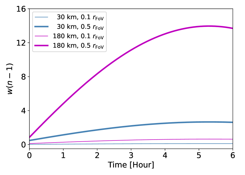
Figure 2: The evolution of $w(n-1)$ term at different parameter combinations. Steel blue and magenta correspond to the baseline lengths of 30 km and 180 km, respectively. Thin and thick lines correspond to the different offsets (as a fraction of FoV radius) to the phase center.

One thing we must pay special attention is the $w$ term. For space VLBI observations that focus on high resolution and are always small field, this term is negligible. However, for wide field imaging, the influence of this term is large and must be taken into account. Fig. 2 demonstrates the contribution of $w$ term to the propagation phase at different distances to the phase center and baseline lengths. For long baselines and large offset (to the phase center), the influence of this term is clearly exhibited. The neglection of $w$ term in FFT method introduces large phase error, which leads to the distortion of the image and the decrease of the dynamic range.

According to Eq. 6, for DFT, it is quite natural to incorporate the contribution of $w$ term into the reconstruction of each pixel and therefore overcomes the difficulties mentioned above. However, compared with FFT method, this method is more computational expensive, which makes it almost unaffordable with a single CPU. Nowadays, with the fast development of modern hardware accelerators, the application of this method in real simulations becomes possible. Moreover, with the aid of modern tensor libraries and computing frameworks, the implementation of the DFT method is rather easy. In the radio imaging part of the current version of OmniUV, Eq. 6 has been implemented using both NumPy and CuPy. The demonstration of this method is presented in Sec. 3.2.

3 Demonstration

The purpose of this section is to demonstrate the capability of OmniUV under different scenarios. Two simulations of quite different scales, namely space VLBI network and wide field array, are presented.

Table 2: Configurations of station for the proposed space VLBI observations in Sec. 3.1. $a$ (semi-major axis), $e$ (eccentricity), $i$ (inclination), $\Omega$ (longitude of the ascending node), $\varpi$ (argument of periapsis) and $M_{0}$ (true anomaly) are the 6 orbital elements for each space telescope.

ID	Station	Description
1	Earth orbit	SEFD =  225 Jy, D =  30 m, $a$ = 6.14$\times 10^{4}$ km, $e$ = 0.73, $i$ =  30∘, $\Omega$ = 0, $\varpi$ = 0, $M_{0}$ = 0
2	Earth orbit	SEFD =  225 Jy, D =  30 m, $a$ = 6.14$\times 10^{4}$ km, $e$ = 0.73, $i$ = -30∘, $\Omega$ = 0, $\varpi$ = 0, $M_{0}$ = 180∘
3	Earth fixed	SEFD =    48 Jy, D =  65 m, TMRT (Tianma Radio Telescope)
4	Earth fixed	SEFD =    20 Jy, D =100 m, Effelsberg Radio Telescope
5	Lunar orbit	SEFD =  507 Jy, D =  20 m, $a$ = 3$\mathrm{R}_{\mathrm{Moon}}$, $e$ = 0, $i$ = 0∘, $\Omega$ = 0, $\varpi$ = 0, $M_{0}$ = 0
6	Lunar fixed	SEFD =2028 Jy, D =  10 m, far side of the Moon
7	Moon-Earth L2	SEFD =  507 Jy, D =  20 m

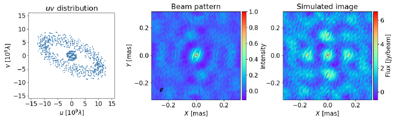
Figure 3: Simulation result for the Moon-Earth network proposed in Sec. 3.1. Left: $uv$ distribution. Middle: beam pattern. Right: reconstructed image. The beam shape derived with TPJ’s algorithm is presented as a black circle in the lower left corner of the middle panel. Beam size: major 0.028 mas, minor 0.011 mas. The input point source distribution is demonstrated in Fig. 5.

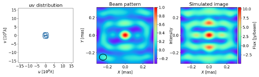
Figure 4: Simulation result for the Earth only network proposed in Sec. 3.1. The meaning of each panel is the same as that in Fig. 3. Beam size: major 0.082 mas, minor 0.070 mas.

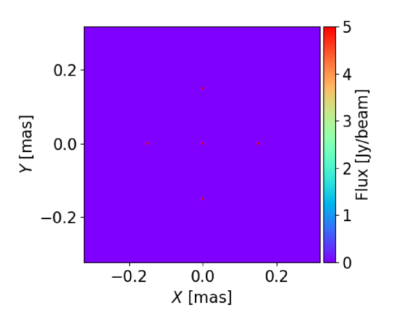
Figure 5: The input structure for space VLBI simulations in Sec. 3.1. 5 point sources with a separation of 0.15 mas are placed in the center of the field of view (FoV). The flux of each point source is set to 5 Jy. Note that the dots in the figure do not indicate the size of ideal “point” sources.

3.1 Space VLBI Network

This simulation demonstrates the improvement of the angular resolution and the image quality with and without the Moon related baselines. The image reconstruction results of the Earth only and the Moon-Earth VLBI network are presented and compared.

The Earth only space VLBI network consists of two ground based and two space stations. For the Moon-Earth network, as a demonstration, three Moon stations, each deployed in the Moon orbit, the farside of the Moon surface and the Moon-Earth L2 point, are included. Tab. 2 presents the detailed configurations of the proposed stations. The main parameters of the observations are: frequency: X band (3.6 cm), phase center: R.A. 180^∘, Dec. 30^∘, bandwidth: 32 MHz, integration time: 2 s, gain error: 0.1.

The source structure is simulated with 5 point sources. The distance between the sources is set such that the source structure could be resolved by both of the Earth only and the Moon-Earth network. As a raw estimation, the baseline length of the Earth only network is in the level of $10^{5}$ km. In the X band, the corresponding angular resolution is about 0.07 mas. As a result, the distance between the sources is set to 0.15 mas.

One thing that we must pay special attention is the schedule of space VLBI observations. For the Earth only network, since there are two ground based stations, to achieve the best $uv$ coverage, the total duration is set to one day, which is the same as the ground only VLBI session. For the Moon-Earth network, we have to realize that the situation is quite different. For one thing, the revolution period of the Moon is one month instead of one day. Moreover, Moon-Earth baselines are much longer than Earth only baselines. Keeping these in mind, we propose the following observation strategy:

• Observations are organized in scans. Each scan lasts for tens of minutes.

• Several scans are arranged within one day.

• Several days are selected for the observation within one month.

This strategy guarantees that the high resolution of Moon-Earth baselines could be fully utilized with relatively good $uv$ coverage. For the observation presented in this section, the configuration is 15 minutes per scan, 2 scans per day with an interval of 12 hours, 28 continuous days.

The input structure is demonstrated in Fig. 5. The simulation results with and without Moon related baselines are presented in Fig. 3 and Fig. 4, respectively. For convenience, the beam size calculated with the TPJ’s algorithm is presented for the beam pattern. Although 5 points could be resolved in both observations, the Moon-Earth network yields much higher angular resolution, and therefore resolves more details. Moreover, the relatively better $uv$ coverage of the Moon-Earth network exhibits smaller side lobe. As a result, the corresponding image is reconstructed with higher quality.

3.2 Wide field array

The simulation of wide field array is based on the planned SKA1-Mid array. For visibility simulation and image construction, DFT method is used, so as to include the contribution of $w$ term and to avoid the artifact of gridding. As pointed out in Sec. 2.3, DFT is computationally expensive. As a result, the number of antennas that take part in observation is constrained: instead of using all antennas in the planned array, 20 out of 190 (15 m diameter) antennas are selected randomly within a radius of 15 km in the central area of the array. The actual size of the array leads to an estimated angular resolution of 13.4 arcsec at 350 MHz. The corresponding pixel size is set to 7.5 arcsec. As a modeling of the neutral hydrogen foreground, 20 point sources with a flux of 1 Jy are placed randomly in the FoV. The main parameters of the observations are: frequency: 350 MHz, phase center: R.A. 180^∘, Dec. -60^∘, bandwidth: 32 MHz, integration time: 2 s, gain error: 0.3, duration: 6 hours.

Fig. 6 presents the simulation result. 20 antennas yield 190 baselines and therefore relatively good $uv$ coverage. We may expect the image quality will be further improved by taking all antennas of SKA1-Mid into account.

One may notice that both scenarios presented in this section are simulations for point sources. Actually we have carried out simulations for diffuse structures as well. The result proves that the source structure could be reconstructed according to the given beam. We hope OmniUV could be used to simulate the 21 cm signal by interferometric observations from HI gas in galaxies in the nearby universe, which is one of the main science goals for SKA1-Mid (Power, 2015). We also realize that since structures smaller than the beam size could not be resolved, the sampling resolution could be set accordingly, so as to reduce the total number of sampling points in the image plane and therefore the amount of computation.

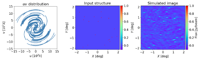
Figure 6: Simulation result for the SKA1-Mid array proposed in Sec. 3.2. Left: $uv$ distribution. Middle: input point source distribution. Right: reconstructed image. Beam size: major 27.9 arcsec, minor 19.6 arcsec. As a modeling of the neutral hydrogen foreground, 20 point sources with a flux of 1 Jy are placed randomly in the FoV. Note that the dots in the middle panel does not indicate the actual size of ideal “point” sources.

4 Future work

As a novel VLBI simulation toolkit, OmniUV is still in its preliminary stage. Several new features are already planned and will be implemented in the near future.

4.1 DRO

With the development of modern space technology, a special kind of orbit, namely DRO (Distant Retrograde Orbit), has obtained more and more attention. DRO is a family of periodic orbits in the circular restricted three-body problem (CR3BP). In the rotating reference frame, it looks like a retrograde orbit around the second body. DRO is proved to be long-term stable, and is therefore regarded as the ideal place for various kinds of space missions. It is necessary to investigate the possibility of the deployment of space VLBI satellite in this orbit. At present, DRO is not yet supported by OmniUV. The main reason is that the object in this orbit is influenced by both the primary and the secondary body, which makes it impossible to derive any analytical solution. As a result, the trajectory of DRO can only be calculated numerically. Zimovan (2017) provides an excellent introduction to DRO and has listed all the possible initial conditions (position and velocity) for the DRO family in the Moon-Earth system. As a next step, a high accuracy numerical integrator will be incorporated to OmniUV, so as to provide the support for the trajectory calculation of DRO and the related visibility and image simulations.

4.2 Performance improvement

The computational complexity of FFT method is low. For most of the space VLBI simulations using this method, the time consumption is already acceptable with only one CPU. However, wide field imaging requires DFT to include the contribution of $w$ term, of which the computational requirement is much higher. The SKA1-Mid simulation presented in Sec. 3.2 takes 5 minutes on 3 GPUs. Note that it includes only 20 antennas within a radius of 15 km in the array center. The actual size of the array is 180 km, which suggests 1 order of magnitude higher angular resolution. The corresponding 2 orders of magnitude increase in the computation requirement is only possible with modern GPU clusters. Therefore, DFT part is planned to be fully parallelized with MPI and accelerated with multiple types of hardware backends.

4.3 Data corruption

A realistic simulation must take various data corruption effects into account. In the current version of OmniUV, the antenna gain and the system noise have been incorporated by following the scheme adopted by Chael et al. (2018). Moreover, for the actual data observation/simulation, the integration over a range of time/frequency will cause the loss of amplitude. This is the well known smearing effect or decoherence. Smirnov (2011) provides a useful first order approximation for this effect. The implementation is relatively easy. However the corresponding time consumption increases significantly. We plan to implement this part when the computation efficiency is not a big issue.

Besides that, at present, the antenna response within the FoV is assumed to be constant. This assumption is reasonable for observations with very long baseline, since the imaging area is significantly smaller than the FoV. However, for wide field array, of which the imaging area is much larger, the variation of antenna response within the FoV must be taken into account, so as to achieve a more realistic result.

5 Summary

In this paper, we present OmniUV, so as to fulfill the requirement of VLBI simulations for both space and ground VLBI observations. It supports various kinds of stations, including Earth (ground) fixed, Earth orbit, Lunar fixed, Lunar orbit, Moon-Earth and Earth-Sun Lagrange 1 and 2 points, etc. The main functionalities of this toolkit are: (1) Trajectory calculation; (2) Baseline $uv$ calculation; (3) Visibility simulation; (4) Image and beam reconstruction.

OmniUV provides two methods for visibility simulation and image reconstruction, namely FFT and DFT. The latter one avoids extra artifacts introduced by the gridding process, so as to achieve the high sensitivity necessary for neutral hydrogen studies. Moreover, $w$ term calculation is naturally supported by this method, which gives OmniUV the ability for simulations of wide field array.

As a demonstration of OmniUV, two scenarios of completely different scales are presented. One is space VLBI, which compares the resolutions of VLBI networks with and without Moon-Earth baselines. Another is ground based SKA1-Mid array, which exhibits the toolkit’s capability of visibility calculation and radio imaging for wide field arrays.

OmniUV is open for access and will be updated continuously. All the necessary documents, examples and packages are publicly available in GitHub repo: https://github.com/liulei/omniuv.

Appendix A Accuracy of $uvw$ calculation

To verify the accuracy of OmniUV $uvw$ calculation, we perform comparison between OmniUV and CALC 9.1. Both calculations are set up for the SKA1-Mid site with identical earth orientation parameters and site coordinate. The result is presented in Fig. 7.

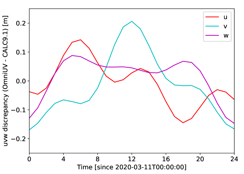
Figure 7: Discrepancy of $uvw$ as a function of time.

According to the figure, the discrepancies are well within 20 cm. We postulate the still existing discrepancy is caused by various types of tide effects which are not taken into account by OmniUV.

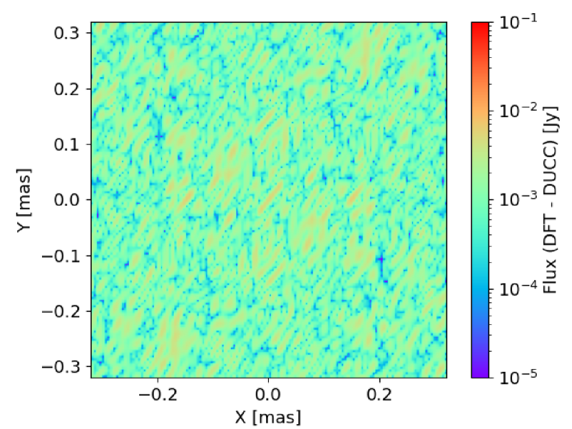
Figure 8: Discrepancy of image reconstruction result between DFT and DUCC lib for the Moon-Earth network simulation in Sec. 3.1.

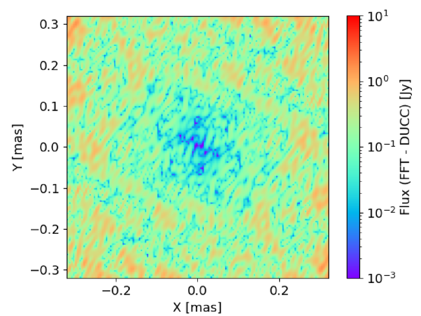
Figure 9: Discrepancy of image reconstruction result between FFT (implemented with nearest neighbour gridding in OmniUV) and DUCC lib for the Moon-Earth network simulation in Sec. 3.1.

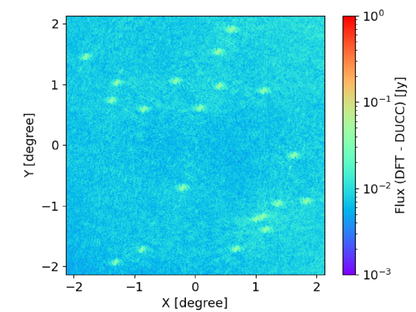
Figure 10: Discrepancy of image reconstruction result between DFT and DUCC lib for the wide field SKA1-Mid simulation in Sec. 3.2.

Appendix B Accuracy of image reconstruction

We compare the image reconstruction results between OmniUV and DUCC lib (Arras et al., 2021). The latter one implements the novel analytical kernel for $uv$ plane gridding, which guarantees high accuracy when transformed to the image plane. The comparisons for the Moon-Earth network are presented in Fig. 8 and 9. Here “FFT” refers to the nearest neighbour gridding method in the current version of OmniUV. Obviously its discrepancy with DUCC lib is much larger than that of the DFT method. The comparison for the SKA1-Mid array is presented in Fig. 10. Compared with the small field imaging in Fig. 8, the discrepancy is relatively larger in the wide field mode. FFT with nearest neighbour gridding is of high efficiency and easy to implement. We keep it in the toolkit to facilitate code development and testing. However, this method is not recommended in the actual application of image reconstruction since its accuracy is low. In general, the accuracy of DUCC lib is as high as DFT, but with less time consumption comparable to FFT (implemented with nearest neighbour gridding in OmniUV) for both small field and wide field imaging. We plan to support DUCC lib in the future release of OmniUV and set it as the default scheme for image reconstruction.

References

- (1)
- Arras et al. (2021) Arras, P., Reinecke, M., Westermann, R., et al. 2021, A&A, 646, A58. doi:10.1051/0004-6361/202039723
- Akiyama et al. (2019) Event Horizon Telescope Collaboration, Akiyama, K., Alberdi, A., et al. 2019, ApJ, 875, L1. doi:10.3847/2041-8213/ab0ec7
- Andrianov et al. (2021) Andrianov, A. S., Baryshev, A. M., Falcke, H., et al. 2021, MNRAS, 500, 4866. doi:10.1093/mnras/staa2709
- Blecher et al. (2017) Blecher, T., Deane, R., Bernardi, G., et al. 2017, MNRAS, 464, 143. doi:10.1093/mnras/stw2311
- Chael et al. (2018) Chael, A. A., Johnson, M. D., Bouman, K. L., et al. 2018, ApJ, 857, 23. doi:10.3847/1538-4357/aab6a8
- Dewdney et al. (2009) Dewdney, P. E., Hall, P. J., Schilizzi, R. T., et al. 2009, IEEE Proceedings, 97, 1482. doi:10.1109/JPROC.2009.2021005
- Dulwich et al. (2009) Dulwich, F., Mort, B. J., Salvini, S., et al. 2009, Wide Field Astronomy & Technology for the Square Kilometre Array, 31
- Hamaker et al. (1996) Hamaker, J. P., Bregman, J. D., & Sault, R. J. 1996, A&AS, 117, 137
- Jaeger (2008) Jaeger, S. 2008, Astronomical Data Analysis Software and Systems XVII, 394, 623
- Kardashev et al. (2014) Kardashev, N. S., Novikov, I. D., Lukash, V. N., et al. 2014, Physics Uspekhi, 57, 1199-1228. doi:10.3367/UFNe.0184.201412c.1319
- Lanman et al. (2019) Lanman, A., Hazelton, B., Jacobs, D., et al. 2019, The Journal of Open Source Software, 4, 1234. doi:10.21105/joss.01234
- Liu (2022) Liu, L. 2022, OmniUV: A Multi-Purpose Simulation Toolkit for VLBI Observation, v1.04, doi:10.5281/zenodo.6619021
- Liu & Zheng (2021) Liu, L. & Zheng, W.-M. 2021, Research in Astronomy and Astrophysics, 21, 037. doi:10.1088/1674-4527/21/2/37
- Noordam & Smirnov (2010) Noordam, J. E. & Smirnov, O. M. 2010, A&A, 524, A61. doi:10.1051/0004-6361/201015013
- Palumbo et al. (2019) Palumbo, D. C. M., Doeleman, S. S., Johnson, M. D., et al. 2019, ApJ, 881, 62. doi:10.3847/1538-4357/ab2bed
- Power (2015) Power, C., Lagos, C., Qin, B., et al. 2015, Advancing Astrophysics with the Square Kilometre Array (AASKA14), 133
- Shepherd (1997) Shepherd, M. C. 1997, Astronomical Data Analysis Software and Systems VI, 125, 77
- Smirnov (2011) Smirnov, O. M. 2011, A&A, 527, A106. doi:10.1051/0004-6361/201016082
- Thompson et al. (2001) Thompson, A. R., Moran, J. M., & Swenson, G. W., Jr. 2001, “Interferometry and synthesis in radio astronomy by A. Richard Thompson, James M. Moran, and George W. Swenson, Jr. 2nd ed. New York : Wiley, c2001.xxiii, 692 p. : ill. ; 25 cm. ”A Wiley-Interscience publication.“ Includes bibliographical references and indexes. ISBN : 0471254924”
- Trott et al. (2012) Trott, C. M., Wayth, R. B., & Tingay, S. J. 2012, ApJ, 757, 101. doi:10.1088/0004-637X/757/1/101
- Zimovan (2017) Zimovan, E. M., 2017, Characteristics and design strategies for near rectilinear halo orbits within the Earth-Moon system (Master dissertation, Purdue University).