Separability of the Hamilton-Jacobi equation and equatorial circular photon orbit in Kerr-Sen-Taub-NUT spacetime

Delvydo Melvernaldo

Center for Theoretical Physics, Department of Physics,

Parahyangan Catholic University, Bandung 40141, Indonesia

In this paper, we show the additive separation of the Hamilton-Jacobi equation, present the 4-velocity of the test particles, and attempt to find the equatorial circular photon orbit (ECPO) in the Kerr-Sen-Taub-NUT (KSTN) solution of the low energy limit of heterotic string theory. In the process of trying to find the ECPO, we instead encounter a ring singularity that could be outside the horizon of the KSTN black hole.

1 Introduction

The Kerr-Sen-Taub-NUT (KSTN) spacetime describes a rotating electrically charged mass with NUT parameter as predicted in the low energy limit of heterotic string theory which is analogous to the Kerr-Newman-Taub-NUT solution of Einstein-Maxwell theory. The author of [1] employed the Hassan-Sen [2] transformation on the Kerr-Taub-NUT (KTN) solution to get the KSTN solution. The Hassan-Sen transformation has been used to map any stationary and axial symmetric spacetime that solves the vacuum Einstein equation to a new solution in the low energy limit of heterotic string theory. The Kerr-Sen solution, which is the solution one would get if the NUT parameter of the KSTN spacetime vanishes, was obtained by Ashoke Sen [3] by applying the Hassan-Sen transformation on the Kerr solution.

In the process of analyzing the behavior of a test particle in a spacetime, the Hamilton-Jacobi formulation is often used to obtain the equations of motion of the test particle [4]. This formulation is particularly useful in finding a conserved quantity in the equations of motion which then can be utilized to simplify the equations. The additive separability of the Hamilton-Jacobi equation (HJE) is critical in finding these conserved quantities. However, Ref. [1] noted that the HJE isn’t likely to be separable due to the presence of a cross-term in the denominator. This impedes the process of calculating the behavior of a test particle in this spacetime.

The organization of this paper is as the followings. In Sect. 2, we provide a short summary of the KSTN solution. In Sect. 3, we separate the HJE of the KSTN solution, find the corresponding conserved quantity, and obtain the 4-velocity of electrically neutral test particles. In Sect. 4, we attempt to find the equatorial circular photon orbit.

2 Kerr-Sen-Taub-NUT spacetime

Using coordinates $x^{\mu}=[t,r,x,\phi]$ where $x=\cos\theta$ in Boyer-Lindquist coordinates, the metric of KSTN spacetime in Einstein frame can be expressed as [1]

$$\begin{split}ds^{2}=&-\frac{\Xi}{\Sigma}\left[\text{d}t-\frac{2M(\Delta_{r}l(1-x)-a\Delta_{x}((M-b)r+l^{2}+al))}{(M-b)\Xi}\text{d}\phi\right]^{2}\\ &+\Sigma\left[\frac{\text{d}r^{2}}{\Delta_{r}}+\frac{\text{d}x^{2}}{\Delta_{x}}+\frac{\Delta_{r}\Delta_{x}\text{d}\phi^{2}}{\Xi}\right]\end{split}$$ (2.1)

with

$$\begin{split}\Sigma&=r(r+2b)+(l+ax)^{2}+\frac{2bl(l+ax)}{M-b},\\ \Xi&=r^{2}-2(M-b)r+a^{2}x^{2}-l^{2},\\ \Delta_{r}&=r^{2}-2(M-b)r+a^{2}-l^{2},\\ \Delta_{x}&=1-x^{2},\end{split}$$ (2.2)

where $M$ is the mass of the gravitating object, $a$ is the rotational parameter, $l$ is the NUT parameter, and the electric charge $Q$ is represented by $b$ with the relation $b=Q^{2}/(2M)$.

The low energy effective action for heterotic string in Einstein frame used for this solution is [5]

$$S=\int d^{4}x\sqrt{-g}\left[R(g)-\frac{1}{2}\nabla_{\mu}\Phi\nabla^{\mu}\Phi-\frac{e^{-\Phi}}{8}F_{\mu\nu}F^{\mu\nu}-\frac{e^{-2\Phi}}{12}H_{\mu\nu\lambda}H^{\mu\nu\lambda}\right]$$ (2.3)

with [1]

$$\begin{split}A_{\mu}\text{d}x^{\mu}=&\ \frac{\sqrt{2}Q}{\sqrt{\Sigma}(M-b)}\left[(alx+l^{2}+(M-b)r)\text{d}t-a\Delta_{x}((M-b)r+l^{2}+al)\text{d}\phi\right],\\ H_{\alpha\beta\mu}=&\ \partial_{\alpha}B_{\beta\mu}+\partial_{\mu}B_{\alpha\beta}+\partial_{\beta}B_{\mu\alpha}-\frac{1}{4}(A_{\alpha}F_{\beta\mu}+A_{\mu}F{\alpha\beta}+A_{\beta}F_{\mu\alpha}),\\ \Phi=&-2\ln\sqrt{\frac{\Sigma}{r^{2}+(l+ax)^{2})}},\end{split}$$ (2.4)

where $A_{\mu}$ is the Maxwell field which gives the field strength tensor $F_{\mu\nu}=\partial_{\mu}A_{\nu}-\partial_{\nu}A_{\mu}2$, $\Phi$ is the dilaton field, $B_{\mu\nu}$ is the second-rank anti-symmetric tensor field, and $H_{\alpha\beta\mu}$ is a Chern-Simons term in the absence of $B_{\mu\nu}$. The non-zero components of $B_{\mu\nu}$ is

$$B_{t\phi}=-B_{\phi t}=\frac{2b}{\sqrt{\Sigma}(M-b)}\left[l\Delta_{r}(1-x)-a\Delta_{x}[(M-b)r+l^{2}+al]\right].$$ (2.5)

Setting $l=0$ reduces the set of fields solutions (2.4) to that of Kerr-Sen [3] and the solution becomes the Kerr-Taub-NUT solution after setting $Q=0$.

Just as Taub-NUT or Kerr-Taub-NUT solutions have conical singularities at the poles where the metric tensor becomes non-invertible [6], the metric (2.1) also has such singularity at $x=-1$. Whether or not the KSTN spacetime has well defined black holes due to this conical defect, one can still find the metric singularities at $\Delta_{r}=0$, i.e.

$$r_{\pm}=M-b\pm\sqrt{(M-b)^{2}+l^{2}-a^{2}}.$$ (2.6)

The frame dragging effect can also be seen in this spacetime where the angular velocity of an observer with constant $r$ and $x$ is

$$\Omega=-\frac{g_{t\phi}}{g_{\phi\phi}}=\frac{-2M\Xi(M-b)\left[a\Delta_{x}[(M-b)r+l^{2}+al]-l\Delta_{r}(1-x)\right]}{4M^{2}\left[a\Delta_{x}[(M-b)r+l^{2}+al]-l\Delta_{r}(1-x)\right]^{2}-\Sigma^{2}(M-b)^{2}\Delta_{r}\Delta_{x}}$$ (2.7)

which at the outermost metric singularity $r_{+}$ reduces to

$$\Omega_{+}=\frac{a(M-b)}{2M(r_{+}(M-b)+l^{2}+al)}.$$ (2.8)

The area covered by the sphere with radius $r_{+}$ can be computed as

$$\mathcal{A}=\int^{2\pi}_{0}\int^{1}_{-1}\sqrt{g_{xx}g_{\phi\phi}}\ \text{d}x\ \text{d}\phi=\frac{8\pi M\left[r_{+}(M-b)+l^{2}+al\right]}{M-b}.$$ (2.9)

3 Hamilton-Jacobi equation separation and equations of motion

Let us consider the Lagrangian

$$2\mathscr{L}=g_{\mu\nu}\dot{x}^{\mu}\dot{x}^{\nu}$$ (3.1)

where the overdot denotes differentiation with respect to an affine parameter $\lambda$ with the normalization condition is $g_{\mu\nu}\dot{x}^{\mu}\dot{x}^{\nu}=\delta$ where one can substitute $\delta=0$ for the null case and $\delta=-1$ for the timelike case. The Hamilton-Jacobi equation (HJE) is

$$g^{\mu\nu}\partial_{\mu}S\partial_{\nu}S=\delta$$ (3.2)

with the Jacobi action ansatz

$$S=-Et+L\phi+S_{r}(r)+S_{x}(x),$$ (3.3)

where $E$ and $L$ are respectively the energy and angular momentum for massless particles but are respectively the specific energy and specific angular momentum for timelike particles. Here, $S_{r}$ and $S_{x}$ are respectively arbitrary functions that depend only on $r$ and $x$. Also notice that

$$\partial_{\mu}S=P_{\mu}=\dot{x}_{\mu}.$$ (3.4)

With that relation, we have

$$E=-g_{t\mu}\dot{x}^{\mu}=\frac{\Xi}{\Sigma}\dot{t}-\frac{2M\left[\Delta_{r}l(1-x)-a\Delta_{x}((M-b)r+l^{2}+al)\right]}{\Sigma(M-b)}\dot{\phi},$$ (3.5)

and

$$\begin{split}L=g_{\phi\mu}\dot{x}^{\mu}=&\frac{2M\left[\Delta_{r}l(1-x)-a\Delta_{x}((M-b)r+l^{2}+al)\right]}{\Sigma(M-b)}\dot{t}\\ &+\left[\frac{\Sigma\Delta_{x}\Delta_{r}}{\Xi}-\frac{4M^{2}\left[\Delta_{r}l(1-x)-a\Delta_{x}((M-b)r+l^{2}+al)\right]^{2}}{\Sigma\Xi(M-b)^{2}}\right]\dot{\phi}.\end{split}$$ (3.6)

Solving equations (3.5) and (3.6), we obtain

$$\begin{split}\dot{t}=&\frac{E}{\Xi}\left[\Sigma-\frac{4M^{2}\left[\Delta_{r}l(1-x)-a\Delta_{x}((M-b)r+l^{2}+al)\right]^{2}}{\Sigma\Delta_{r}\Delta_{x}(M-b)^{2}}\right]\\ &+\frac{2M\left[\Delta_{r}l(1-x)-a\Delta_{x}((M-b)r+l^{2}+al)\right]}{\Sigma\Delta_{x}\Delta_{r}(M-b)}L,\end{split}$$ (3.7)

and

$$\dot{\phi}=\frac{\Xi L}{\Sigma\Delta_{x}\Delta_{r}}-\frac{2M\left[\Delta_{r}l(1-x)-a\Delta_{x}((M-b)r+l^{2}+al)\right]}{\Sigma\Delta_{x}\Delta_{r}(M-b)}E.$$ (3.8)

With the Jacobi action ansatz (3.3), the metric (2.1), and the additive separation of variables algorithm explained in appendix A, the HJE (3.2) becomes

$$\begin{split}\Sigma\ \delta=&\Delta_{r}\left(\partial_{r}S_{r}(r)\right)^{2}+\Delta_{x}\left(\partial_{x}S_{x}(x)\right)^{2}+\left[\frac{1}{\Delta_{x}}-\frac{a^{2}}{\Delta_{r}}\right]L^{2}\\ &-2\left[\frac{F_{x}}{\Delta_{x}}-\frac{F_{r}}{\Delta_{r}}\right]EL+\left[\frac{\psi_{x}}{\Delta_{x}}-\frac{\psi_{r}}{\Delta_{r}}\right]E^{2}\end{split}$$ (3.9)

where

$$\begin{split}F_{x}=&\frac{2Ml(1-x)}{M-b}-\Delta_{x}\left[\frac{2Ml}{M-b}\right],\\ F_{r}=&\frac{2Ma[(M-b)r+l^{2}+al]}{M-b}-\Delta_{r}\left[\frac{2Ml}{M-b}\right],\\ \psi_{x}=&\frac{8M^{2}l^{2}(1-x)x}{(M-b)^{2}}-\Delta_{x}\left[a^{2}x^{2}+\frac{4Malx}{M-b}\right],\\ \psi_{r}=&4M^{2}\left[2r\left(M-b+\frac{l^{2}+al}{M-b}\right)-(a^{2}-l^{2})+\left(\frac{a+l}{M-b}\right)^{2}l^{2}\right]\\ &+\Delta_{r}\left[r^{2}+2r(M+b)+4M^{2}-\left(\frac{M+b}{M-b}\right)^{2}l^{2}\right].\end{split}$$ (3.10)

The separability of the HJE implies the existence of a conserved quantity termed as the Carter constant $K$ [7] where

$$\Delta_{x}(\partial_{x}S_{x})^{2}+\frac{x^{2}}{\Delta_{x}}L^{2}-\frac{2F_{x}}{\Delta_{x}}EL+\frac{\psi_{x}}{\Delta_{x}}E^{2}-\left[\frac{2Malx}{M-b}+a^{2}x^{2}\right]\delta=K,$$ (3.11)

and

$$\Delta_{r}(\partial_{r}S_{r})^{2}+\left[1-\frac{a^{2}}{\Delta_{r}}\right]L^{2}+\frac{2F_{r}}{\Delta_{r}}EL-\frac{\psi_{r}}{\Delta_{r}}E^{2}-\left[r(r+2b)+\frac{l^{2}(M+b)}{M-b}\right]\delta=-K.$$ (3.12)

Using the relation (3.4), we get

$$\Sigma\dot{x}=\pm\sqrt{\mathcal{X}},$$ (3.13)

$$\Sigma\dot{r}=\pm\sqrt{\mathcal{R}},$$ (3.14)

with

$$\mathcal{X}=\mathcal{X}(x)= -x^{2}L^{2}+F_{x}EL-\psi_{x}E^{2}+\Delta_{x}\left[K+\left(\frac{2Malx}{M-b}+a^{2}x^{2}\right)\delta\right],$$ (3.15)

$$\mathcal{R}=\mathcal{R}(r)= a^{2}L^{2}-F_{r}EL+\psi_{r}E^{2}-\Delta_{r}\left[K+L^{2}-\left(r(r+2b)+\frac{l^{2}(M+b)}{M-b}\right)\delta\right].$$ (3.16)

The $\pm$ signs in equations (3.13) and (3.14) are independent from each other but must stay consistent once the signs are chosen. The $+$($-$) sign in equation (3.14) denotes the outgoing(ingoing) geodesics. Just as in [8, 9, 10], one can introduce a new time parameter $\sigma$ such that

$$\frac{\text{d}\sigma}{\text{d}\lambda}=\frac{1}{\Sigma}.$$ (3.17)

With this new parameter and equations (3.13) and (3.14), we can use $\mathcal{R}$ and $\mathcal{X}$ as the effective potentials in $r$ and $x$

$$\left(\frac{\text{d}r}{\text{d}\sigma}\right)^{2}= \ \mathcal{R}(r),$$ (3.18)

$$\left(\frac{\text{d}x}{\text{d}\sigma}\right)^{2}= \ \mathcal{X}(x).$$ (3.19)

The effective potential $\mathcal{R}(r)$ can also be written in the polynomial form

$$\mathcal{R}(r)=f_{4}r^{4}+f_{3}r^{3}+f_{2}r^{2}+f_{1}r+f_{0}$$ (3.20)

where

$$f_{4}= \ E^{2}+\delta,$$ (3.21)

$$f_{3}= \ 2\left[2bE^{2}-(M-2b)\delta\right],$$ (3.22)

$$\begin{split}f_{2}=&\ E^{2}\left(4b^{2}-2l^{2}+a^{2}\right)+4lLE-K-\frac{4bl^{2}E^{2}}{M-b}-\left[\frac{2blE}{M-b}-L\right]^{2}\\ &\ +\left[a^{2}+\frac{2bl^{2}}{M-b}-4b(M-b)\right]\delta,\end{split}$$ (3.23)

$$\begin{split}f_{1}=&\ 2(M-b)\left[(L-aE-2El)^{2}+K\right]+4b\left[a^{2}E^{2}+(4al+5l^{2})E^{2}-(a+2l)LE\right]\\ &\ +\frac{8b^{2}l(a+2l)E^{2}}{M-b}+2\left[b(a^{2}-3l^{2})-l^{2}(M-b)\right]\delta,\end{split}$$ (3.24)

$$\begin{split}f_{0}=&\ \left[(a+l)(3a+5l)E^{2}-4(a+l)LE+L^{2}+K\right]l^{2}-Ka^{2}+\frac{8b^{2}l^{3}(a+l)E^{2}}{(M-b)^{2}}\\ &\ +\frac{4bl^{2}E(a+l)}{M-b}\left[3lE+aE-L\right]+l^{2}(a^{2}-l^{2})\left[\frac{M+b}{M-b}\right]\delta.\end{split}$$ (3.25)

By looking at the coefficient of the highest order of $r$, notice that the motion can be unbounded ($r\to\infty$) if $E^{2}>-\delta$. For $E^{2}<-\delta$, the motion is bounded and cannot diverge to infinity. For the case $E^{2}=-\delta$, whether the motion is finite or infinite depends on the other parameters for the allowed regions and is said to be marginally bounded.

4 Equatorial circular photon orbit

Since we will be discussing photons, let us immediately use $\delta=0$ for the rest of this section. I will first consider the constraints necessary for a photon to move over the equatorial plane $x=0$, namely

$$\mathcal{X}|_{x=0}=K=0$$ (4.1)

and

$$\left.\frac{\text{d}\mathcal{X}}{\text{d}x}\right|_{x=0}=\frac{\left[8M^{2}lE^{2}+4ME(aE-L)\right]l}{(M-b)^{2}}=0.$$ (4.2)

One can see that the constraint (4.2), which corresponds to the acceleration in $x$, is satisfied for zero NUT parameter. For non-zero NUT parameter, we have an additional constrain for the energy and angular momentum of the particle. The value of the particle’s angular momentum $L$ that satisfies the latter constraint, i.e. Eq. (4.2), is

$$L=aE+\frac{2EMl}{M-b}.$$ (4.3)

I will use these values for $K$ and $L$ from equations (4.1) and (4.3) for the rest of this section. Since the inequality

$$\left.\frac{\text{d}^{2}\mathcal{X}}{\text{d}x^{2}}\right|_{x=0}=-\frac{8M^{2}l^{2}E^{2}}{(M-b)^{2}}<0$$ (4.4)

is satisfied, this motion over the equatorial plane is stable, i.e. small perturbations in the $x$ direction will not throw the particle away from the equator.

Next, let us consider the constraints for circular motion, namely

$$\mathcal{R}|_{r=r_{c}}=E^{2}\left[r_{c}(r_{c}+2b)+\frac{l^{2}(M+b)}{(M-b)}\right]^{2}=0$$ (4.5)

and

$$\left.\frac{\text{d}\mathcal{R}}{\text{d}r}\right|_{r=r_{c}}=4E^{2}(r_{c}+b)\left[r_{c}(r_{c}+2b)+\frac{l^{2}(M+b)}{M-b}\right]=0.$$ (4.6)

Notice that the expression inside the bracket on both equations (4.5) and (4.6) is in fact $\Sigma|_{x=0,r=r_{c}}$. From the Kretchmann scalar $R_{\alpha\beta\mu\nu}R^{\alpha\beta\mu\nu}$ at the equatorial plane, which is

$$\left.R_{\alpha\beta\mu\nu}R^{\alpha\beta\mu\nu}\right|_{x=0}=\frac{\mathcal{O}(r^{6})}{\left[(M-b)\Sigma|_{x=0}\right]^{6}},$$ (4.7)

one can see that $\Sigma|_{x=0}=0$ would make the curvature scalar singular. Looking into this further, if we solve Eq. (4.5) for $r_{c}$ with $E\neq 0$ regardless of the curvature singularity, we get

$$r_{c}=-b\pm\sqrt{b^{2}-\frac{l^{2}(M+b)}{M-b}}.$$ (4.8)

It is interesting to notice that $r_{c}$ is positive if and only if $M<b$ and this can theoretically be achieved while still maintaining the reality of the horizon $r_{+}$. We can also find a set of parameters that satisfies $r_{c}>r_{+}$.

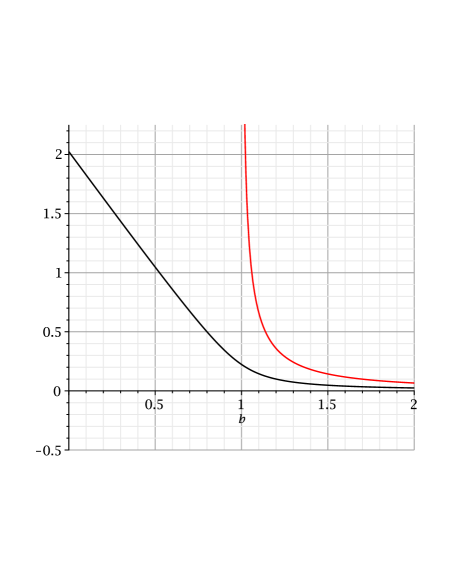
Figure 1: Plot of $r_{c}$ (red) and the outter horizon $r_{+}$ (black) with varying values of $b$ with $M=1$, $l=0.3$, and $a=0.2$.

As an example, figure 1 shows the plot of $r_{c}$ alongside the outter horizon $r_{+}$ with varying $b$, where the spacetime parameters being used are $M=1$, $l=0.3$, and $a=0.2$. This means there could be a ring singularity at the equator with $r=r_{c}$ outside the horizon $r_{+}$ if $M<b$. This could be another condition for the ”cosmic censorship hypothesis” to be aware of in KSTN spacetime other than the $r_{+}\in\mathbb{R}$ condition, at least for $x=0$ case. Also, it can be seen that, in a case of extremal KSTN black hole, the horizon radius $r_{+}$ is negative if $M<b$ is satisfied. Although as interesting as it is, further discussion on the nature of the singularities in this spacetime is outside the scope of this paper.

5 Conclusion

In this paper, we obtain another conserved quantity known as the Carter constant by separating the Hamilton-Jacobi Equation for the Kerr-Sen-Taub-NUT spacetime. This metric was obtained and its properties were originally studied in [1].

In Sect. 4, we also searched for equatorial circular photon orbits (ECPO) utilizing the Carter constant obtained in Sect. 3. In the process, we instead found another ring singularity that could appear outside the horizon $r_{+}$ if $M<b$, which is needed for the ECPO to be outside the horizon as well. Analyzing the geodesics in KSTN spacetime as well as examining the Banados-Silk-West [11, 12] effect in KSTN spacetime are the future projects that can be done related to the KSTN solution.

Appendix A Additive separation of variables algorithm

Here I will discuss the algorithm used to do an additive separation of variables on a multivariate function, in particular, a function that depends on two variables. Suppose we have the function $F(x,y)$ which we want to rewrite as

$$F(x,y)=f(x)+g(y).$$ (A.1)

As the author of [13] showed, the relation

$$\partial_{x}\partial_{y}F(x,y)=\partial_{y}\partial_{x}F(x,y)=0$$ (A.2)

must be true. Using the fact that a function can be expressed as

$$f(x)=\int{\frac{\text{d}f(x)}{\text{d}x}\text{d}x}+C,$$ (A.3)

and

$$\begin{split}\partial_{x}F(x,y)=\frac{\text{d}f(x)}{\text{d}x},\\ \partial_{y}F(x,y)=\frac{\text{d}g(y)}{\text{d}y},\end{split}$$ (A.4)

the function $F(x,y)$ can be written as

$$F(x,y)=\int{\partial_{x}F(x,y)\text{d}x}+\int{\partial_{y}F(x,y)\text{d}y}+C$$ (A.5)

where the first term and the second term are respectively functions that only depend on $x$ and $y$, achieving the additive separation of variables. The appropriate constant $C$ is chosen to make the relation (A.5) true.

References

[1]
H. M. Siahaan,
Eur. Phys. J. C 80 (2020),
doi:10.1140/epjc/s10052-020-08561-z.
[2]
S. Hassan and A. Sen,
Nuclear Physics B 375, 103 (1992),
doi:10.1016/0550-3213(92)90336-a.
[3]
A. Sen,
Phys. Rev. Lett. 69, 1006 (1992),
doi:10.1103/physrevlett.69.1006.
[4]
C. Dewitt and B. S. Dewitt,
Black Holes (Les Astres Occlus) (1973).
[5]
C. V. Johnson and R. C. Myers,
Phys. Rev. D 50, 6512 (1994),
doi:10.1103/physrevd.50.6512.
[6]
Y. C. Ong,
Journal of Cosmology and Astroparticle Physics 2017, 001
(2017),
doi:10.1088/1475-7516/2017/01/001.
[7]
B. Carter,
Commun.Math. Phys. 10, 280 (1968),
doi:10.1007/bf03399503.
[8]
H. Cebeci, N. Özdemir, and S. Şentorun,
Gen Relativ Gravit 51, 85 (2019),
doi:10.1007/s10714-019-2569-3.
[9]
A. F. Zakharov,
Monthly Notices of the Royal Astronomical Society 269, 283
(1994),
doi:10.1093/mnras/269.2.283.
[10]
Y. Mino,
Phys. Rev. D 67 (2003),
doi:10.1103/physrevd.67.084027.
[11]
M. Bañados, J. Silk, and S. M. West,
Phys. Rev. Lett. 103, 111102 (2009),
doi:10.1103/physrevlett.103.111102.
[12]
A. Zakria and M. Jamil,
J. High Energ. Phys. 2015, 147 (2015),
doi:10.1007/jhep05(2015)147.
[13]
Y. Cherniavsky,
International Journal of Mathematical Education in Science and
Technology 42, 129 (2011),
doi:10.1080/0020739x.2010.519793.