Higher order graded mesh scheme for time fractional differential equations

Abstract

In this article, we propose a $\left(3-\alpha\right)^{\text{th}},\alpha\in(0,1)$ order approximation to Caputo fractional (C-F) derivative using graded mesh and standard central difference approximation for space derivatives, in order to obtain the approximate solution of time fractional partial differential equations (TFPDE). The proposed approximation for C-F derivative tackles the singularity at origin effectively and is easily applicable to diverse problems. The stability analysis and truncation error bounds of the proposed scheme are discussed, along with this, analyzed the required regularity of the solution. Few numerical examples are presented to support the theory.

MSC: 65L05
Keywords: Graded mesh, Fractional differential equations, nonlinear problem, Initial value problems, L1 scheme

1 Introduction

The study of time fractional differential equations is very intense in the past decade due to its applications in various interdisciplinary areas, a detailed review has been presented in [1]. For the sake of presentation, in the following we study the constant coefficient TFPDE, which is of the form:

$${}_{0}^{C}D_{t}^{\alpha}y(x,t)=a\dfrac{\partial^{2}y(x,t)}{\partial x^{2}}+cy(x,t)+f(x,t),\quad\left(x,t\right)\in\left(0,X\right)\times(0,T],\,\alpha\in\left(0,1\right),a>0,c\leq 0$$ (1.1)

$$y(x,0)=\phi(x),\ x\in\left(0,X\right)$$ (1.2)

$$y(0,t)=\psi_{0}(t),\;y(X,t)=\psi_{X}(t),\ t\in(0,T].$$ (1.3)

Well adapted approximation of C-F derivative in the study of FDE is the standard L1 scheme [2, 3] which is a $\left(2-\alpha\right)^{\text{th}}$ order approximation, the authors of [4] discussed an extension to standard L1 scheme which is a $\left(3-\alpha\right)^{\text{th}}$ order approximation. The authors in [2, 3, 4], while approximating the C-F derivative, did not consider the weak singularity occurring at origin for the study of convergence of the numerical scheme. Stynes et al., [5] discussed the numerical solution of TFPDE using standard L1 approximation on graded mesh. This is one of the earliest articles to discuss the convergence analysis of the method taking into consideration the initial weak singularity. Very recently, Ren et al. in their article [6] constructed a scheme based on the L1-type formula on graded mesh in time and the direct discontinuous Galerkin in space directions for solving TFPDE. Zheng et al. in [7] presented a scheme for solving the 2D multi-term time-fractional diffusion equation with non-smooth solutions, where L1-type formula is derived on graded mesh for approximating the C-F time derivative and Legendre spectral approximation is used for the space derivatives.

In the following, we first state in brief the regularity requirement for the solution of (1.1)-(1.3), i.e., in section 2. In section 3, a numerical scheme is proposed based on the approximation of the C-F derivative using second order non-uniform finite differences and standard central differences for space derivatives. Stability analysis and truncation error bounds are studied in section 4. Scrutinized few examples for the applicability of the scheme in section 5.

2 Regularity

The series solution of TFPDE (1.1)-(1.3) is well discussed in [8] by using the variable separable technique, the associated Strum-Liouville problem is

$$\mathcal{L}p:=\left(-a\dfrac{d^{2}}{dx^{2}}-c\right)p=\lambda p;p(0)=0=p(X)$$

Let $\lambda_{l}(>0)\text{ and }\theta_{l},l=1,2,\cdots$ be the eigen values and normalised eigen functions respectively of this problem.

Based on the concepts of fractional sectorial operators, the domain of $\mathcal{L^{\gamma}}$ is defined as

$$D\left(\mathcal{L}^{\gamma}\right):=\left\{f\in L_{2}\left(0,X\right):\sum_{l=1}^{\infty}\lambda_{l}^{2\gamma}\left|\left\langle f,\theta_{l}\right\rangle\right|^{2}<\infty\right\}.$$

Let us define $\left\|f\right\|_{\mathcal{L}^{\gamma}}:=\left({\displaystyle\sum_{l=1}^{\infty}}\lambda_{l}^{2\gamma}\left|\left\langle f,\theta_{l}\right\rangle\right|^{2}\right)^{\frac{1}{2}}.$ Here $\left\langle.,.\right\rangle$ represents the standard scalar product in $L_{2}\left(0,X\right).$

The series solution for (1.1)-(1.3) with homogeneous boundary conditions is given by

$$y(x,t)=\sum_{l=1}^{\infty}\left[\left\langle\phi,\theta_{l}\right\rangle E_{\alpha,1}\left(-\lambda_{l}t^{\alpha}\right)+\int_{0}^{t}s^{\alpha-1}E_{\alpha,\alpha}\left(-\lambda_{l}t^{\alpha}\right)f_{l}(t-s)ds\right]\theta_{l}\left(x\right),$$

where $f_{l}(s):=\left\langle f\left(\cdot,s\right),\theta_{l}\left(\cdot\right)\right\rangle$ and $E_{\alpha,\beta}$ is the Mittag-Leffler function defined by

$$E_{\alpha,\beta}\left(s\right):={\displaystyle\sum_{k=0}^{\infty}}\dfrac{s^{k}}{\Gamma\left(\alpha k+\beta\right)}.$$

In what follows, we state the theorem pertaining to the regularity of the solution of (1.1)-(1.3). The proof of this theorem can be obtained on similar lines to the proof of Theorem 2.1 of [5].

Theorem 2.1

Suppose $\phi\in D\left(\mathcal{L}^{7/2}\right)$, $f\in D\left(\mathcal{L}^{5/2}\right),$ $f_{t},f_{tt}\in D\left(\mathcal{L}^{1/2}\right)$ and

$$\left\|f\left(.,t\right)\right\|_{\mathcal{L}^{5/2}}+\left\|f_{t}\left(.,t\right)\right\|_{\mathcal{L}^{1/2}}+\left\|f_{tt}\left(.,t\right)\right\|_{\mathcal{L}^{1/2}}+t^{\mu}\left\|f_{ttt}\left(.,t\right)\right\|_{\mathcal{L}^{1/2}}\leq K_{1},$$

for all $t\in(0,T].$ Here, constant $K_{1}$ is not dependent on $t$ and $\mu<1$ is an arbitrary constant. Then, the TFPDE with homogeneous boundary conditions (1.1)-(1.3) has a unique solution $y(x,t)$ (satisfies the the differential equation and the initial condition, point-wise), and $\exists\ K_{2}$ a constant $\ni$

$$\begin{split}\left|\dfrac{\partial^{p}y}{\partial x^{p}}\left(x,t\right)\right|&\leq K_{2},\ p=0,1,2,3,4,\\ \left|\dfrac{\partial^{p}y}{\partial t^{p}}\left(x,t\right)\right|&\leq K_{2}\left(1+t^{\alpha-p}\right),\ p=0,1,2,3,\end{split}\ \forall\left(x,t\right)\in[0,X]\times(0,T].$$

3 Numerical scheme

Suppose $M,N\in\mathbb{\mathbb{Z}^{+}}/\{0\}$ be the number of sub-intervals in space and time direction respectively of the domain $\left(0,X\right)\times(0,T].$ The points in space are equidistant and in time direction are graded. Let $\left(x_{m},t_{j}\right)$ be the discrete point in the domain, we took $x_{0}=0,x_{m}=mh,x_{M}=X,t_{0}=0,t_{j}=\left(\frac{j}{N}\right)^{\beta}T,t_{N}=T.$ Here $\beta\in\mathbb{R^{+}}/\{0\}.$

First we take note on the approximation of C-F time derivative.

3.1 Approximation of C-F derivative

A higher order approximation for C-F derivative to the function $u(t)$ is obtained using a modification to the standard L1 scheme. From the definition of C-F derivative to $u(t)$ at $t=t_{j},$ we’ve

$$\begin{split}{}_{0}^{C}D_{t}^{\alpha}u(t_{j})&=\frac{1}{\Gamma(1-\alpha)}{\displaystyle\int_{0}^{t_{j}}}(t_{j}-\eta)^{-\alpha}u^{\prime}(\eta)d\eta=\sum_{k=0}^{j-1}{\displaystyle\int_{t_{k}}^{t_{k+1}}}\dfrac{(t_{j}-\eta)^{-\alpha}}{\Gamma(1-\alpha)}u^{\prime}(\eta)d\eta=:\sum_{k=0}^{j-1}S_{k,j}.\end{split}$$ (3.1)

Considering the second order nonuniform finite difference approximation for $u^{\prime}(t_{k}),u^{\prime\prime}(t_{k})$ in the Taylor’s expansion for $u^{\prime}$ taken as

$$u^{\prime}(\eta)=u^{\prime}(t_{k})+\frac{(\eta-t_{k})}{1!}u^{\prime\prime}(t_{k})+\frac{(\eta-t_{k})^{2}}{2!}u^{\prime\prime\prime}(t_{k})+\mathcal{O}\left((\eta-t_{k})^{3}\right),\quad t_{k}\leq\eta\leq t_{k+1},$$

upon simplifying we get

$$S_{k,j}= \frac{1}{\Gamma(1-\alpha)}{\displaystyle\int_{t_{k}}^{t_{k+1}}}(t_{j}-\eta)^{-\alpha}\Bigg{(}\dfrac{u\left(t_{k+1}\right)-u\left(t_{k-1}\right)}{\tau_{k+1}+\tau_{k}}-\dfrac{\tau_{k+1}-\tau_{k}}{2}u^{\prime\prime}(t_{k})$$

$$+2(\eta-t_{k})\left[\dfrac{u\left(t_{k+1}\right)}{\tau_{k+1}\left(\tau_{k+1}+\tau_{k}\right)}-\dfrac{u\left(t_{k}\right)}{\tau_{k+1}\tau_{k}}+\dfrac{u\left(t_{k-1}\right)}{\tau_{k}\left(\tau_{k+1}+\tau_{k}\right)}\right]\Bigg{)}d\eta+Tr_{k,j},$$

$$=2\delta_{k,j}\left[\dfrac{u^{k+1}}{\tau_{k+1}\left(\tau_{k+1}+\tau_{k}\right)}-\dfrac{u^{k}}{\tau_{k+1}\tau_{k}}+\dfrac{u^{k-1}}{\tau_{k}\left(\tau_{k+1}+\tau_{k}\right)}\right]+\gamma_{k,j}\left[\dfrac{u^{k+1}-u^{k-1}}{\tau_{k+1}+\tau_{k}}\right]+Tr_{k,j},$$ (3.2)

where $Tr_{k,j}$ is the truncation error, $u^{k}\approxeq u\left(t_{k}\right)$, $\tau_{k}=t_{k}-t_{k-1}$. Observe that for $k=0$ in equation (3.2) we lack the information for $u^{-1},$ to avoid this scenario $S_{0,j}$ is approximated separately. Initially for approximating $S_{0,1}$, to be of order $\left(3-\alpha\right)$ the interval $\left[0,t_{1}\right]$ is divided into $\overline{N}$ sub intervals such that $\overline{N}^{\alpha-2}\approx N^{\alpha-3}t_{1},$ with $0=\overline{t}_{0}<\overline{t}_{1}<\overline{t}_{2}<\cdots<\overline{t}_{\overline{N}}=t_{1},$ and using the graded standard L1 approximation

$$\begin{split}S_{0,1}&={\displaystyle\sum_{k=0}^{\overline{N}-1}{\displaystyle\int_{\overline{t}_{k}}^{\overline{t}_{k+1}}}}\dfrac{(t_{1}-\eta)^{-\alpha}}{\Gamma(1-\alpha)}u^{\prime}(\eta)d\eta=-\zeta_{0,\overline{N}}u^{(0)}+\sum_{k=1}^{\overline{N}-1}u^{(k)}\left(\zeta_{k-1,\overline{N}}-\zeta_{k,\overline{N}}\right)+\zeta_{\overline{N}-1,\overline{N}}u^{(\overline{N})}+Tr_{1},\end{split}$$

where $u^{(k)}\approxeq u\left(\overline{t}_{k}\right)$ and $\zeta_{k,\overline{N}}=\frac{\left(\overline{t}_{\overline{N}}-\overline{t}_{k}\right)^{1-\alpha}-\left(\overline{t}_{\overline{N}}-\overline{t}_{k+1}\right)^{1-\alpha}}{\Gamma(2-\alpha)\left(\overline{t}_{k+1}-\overline{t}_{k}\right)}.$

Similarly, $S_{0,j},j\geq 2$ occurring in (3.1) is also approximated using the graded standard L1 scheme as above. Now,

$${}_{0}^{C}D_{t}^{\alpha}u(t_{j}) =S_{0,j}+\sum_{k=1}^{j-1}S_{k,j}=-\xi_{0,j}u^{(0)}+\sum_{k=1}^{\overline{N}-1}u^{(k)}\left(\xi_{k-1,j}-\xi_{k,j}\right)+\xi_{\overline{N}-1,j}u^{(\overline{N})}$$

$$+\sum_{k=1}^{j-1}\left(\gamma_{k,j}\left[\dfrac{u^{k+1}-u^{k-1}}{\tau_{k+1}+\tau_{k}}\right]+2\delta_{k,j}\left[\dfrac{u^{k+1}}{\tau_{k+1}\left(\tau_{k+1}+\tau_{k}\right)}-\dfrac{u^{k}}{\tau_{k+1}\tau_{k}}+\dfrac{u^{k-1}}{\tau_{k}\left(\tau_{k+1}+\tau_{k}\right)}\right]\right)+Tr_{j},$$

where $\xi_{k,j}=\frac{\left(t_{j}-\overline{t}_{k}\right)^{1-\alpha}-\left(t_{j}-\overline{t}_{k+1}\right)^{1-\alpha}}{\Gamma(2-\alpha)\left(\overline{t}_{k+1}-\overline{t}_{k}\right)}.$

3.2 Derivation of the method

Consider the discrete equation of (1.1) at $\left(x_{m},t_{j}\right)$

$${}_{0}^{C}D_{t}^{\alpha}y(x_{m},t_{j})=a\dfrac{\partial^{2}y(x_{m},t_{j})}{\partial x^{2}}+cy(x_{m},t_{j})+f(x_{m},t_{j}),\ 1\leq m\leq M-1,1\leq j\leq N.$$

Replacing the approximation of the C-F derivative as discussed in the previous subsection, central difference approximation for the space derivative and upon simplification we get at $t=t_{1}$

$$\begin{split}&-y\left(x_{m-1},t_{1}\right)\dfrac{a}{h^{2}}+y\left(x_{m},t_{1}\right)\left[\zeta_{\overline{N}-1,\overline{N}}+\dfrac{2a}{h^{2}}-c\right]-y\left(x_{m+1},t_{1}\right)\dfrac{a}{h^{2}}\\ =&\zeta_{0,\overline{N}}y\left(x_{m},\overline{t}_{0}\right)+\sum_{k=1}^{\overline{N}-1}y\left(x_{m},\overline{t}_{k}\right)\left(\zeta_{k,\overline{N}}-\zeta_{k-1,\overline{N}}\right)+f\left(x,t_{1}\right)+Tr_{1}+\mathcal{O}\left(h^{2}\right)\end{split}$$ (3.3)

and for $t=t_{j},\ j\geq 2$

$$-y\left(x_{m-1},t_{j}\right)\dfrac{a}{h^{2}}+y\left(x_{m},t_{j}\right)\left[d_{j,j}+\dfrac{2a}{h^{2}}-c\right]-y\left(x_{m+1},t_{j}\right)\dfrac{a}{h^{2}}$$

$$= \xi_{0,j}y\left(x_{m},\overline{t}_{0}\right)+\sum_{k=1}^{\overline{N}-1}y\left(x_{m},\overline{t}_{k}\right)\left(\xi_{k,j}-\xi_{k-1,j}\right)-\xi_{\overline{N}-1,j}y\left(x_{m},\overline{t}_{\overline{N}}\right)+\sum_{k=0}^{j-1}d_{k,j}y\left(x_{m},t_{k}\right)+f\left(x_{m},t_{j}\right)+\mathcal{O}\left(h^{2}\right)+Tr_{j}.$$

4 Stability analysis

We discuss the stability of the proposed scheme for solving TFPDE using Von-Neumann stability analysis. To do so, considered $\delta_{m}^{(J)}=z_{m}^{(J)}-y_{m}^{(J)}\text{ and }\ \delta_{m}^{j}=z_{m}^{j}-y_{m}^{j}$ $\ 0\leq m\leq M,\ 0\leq J\leq\overline{N}\ 0\leq j\leq N$ respectively the difference between the perturbed and approximate solutions (perturbation is due to a small variation in the initial condition) of the proposed scheme as given in (3.3) and (3.2). Replacing $\delta_{m}^{(J)}=\mu^{(J)}e^{i\rho mh}$ and $\delta_{m}^{j}=\mu^{j}e^{i\rho mh}$ where $\rho$ is the spatial wave number, $\mu$ is the amplitude and $i^{2}=-1,$ in (3.3) and (3.2) respectively, we get

$$\mu^{(\overline{N})}\overline{D}_{\overline{N}}=\zeta_{0,\overline{N}}\mu^{(0)}+\sum_{k=1}^{\overline{N}-1}\mu^{(k)}\left(\zeta_{k,\overline{N}}-\zeta_{k-1,\overline{N}}\right),$$

$$\mu^{j}D_{j}=\sum_{k=0}^{j-1}d_{k,j}\mu^{k}+\xi_{0,j}\mu^{(0)}+\sum_{k=1}^{\overline{N}-1}\mu^{(k)}\left(\xi_{k,j}-\xi_{k-1,j}\right)-\xi_{\overline{N}-1,j}\mu^{(\overline{N})}.$$ (4.1)

Further, for the stability of the scheme at $t=\overline{t}_{\overline{N}}=t_{1},$ one needs to analyze the intermediate calculations leading to (3.3) for which we have

$$\mu^{(J)}\overline{D}_{J}=\zeta_{0,j}\mu^{(0)}+\sum_{k=1}^{J-1}\mu^{(k)}\left(\zeta_{k,J}-\zeta_{k-1,J}\right).$$ (4.2)

Where $D_{j}=d_{j,j}-c+\dfrac{a\sin^{2}\left(\rho h/2\right)}{h^{2}},\ 1\leq j\leq N,$ $\overline{D}_{J}=\zeta_{J-1,J}-c+\dfrac{a\sin^{2}\left(\rho h/2\right)}{h^{2}},\ 1\leq J\leq\overline{N}.$

Note that $\overline{D}_{J}\geq\zeta_{J-1,J}\ \text{and\ }D_{j}\geq d_{j,j},$ holds true.

Lemma 4.1

$\left(a\right)$ For every $J\geq 1,$ $\zeta_{k-1,J}$$\leq\zeta_{k,J},$ $\forall k<J.$ $\left(b\right)$ For every $j\geq 2,$ ${\displaystyle\sum_{k=0}^{j-1}}d_{k,j}=d_{j,j}.$

Theorem 4.1

For every $1\leq J\leq\overline{N}$ and for $2\leq j\leq N$ respectively we have

$$\left|\mu^{(J)}\right|\leq\left|\mu^{0}\right|\text{ and }\left|\mu^{j}\right|\leq\left|\mu^{0}\right|.$$ (4.3)

Proof: Define $\overline{\zeta}_{J}=\dfrac{\zeta_{0,J}+{\displaystyle\sum_{k=1}^{J-1}}\left(\zeta_{k,J}-\zeta_{k-1,J}\right)\overline{\zeta_{k}}}{\overline{D}_{J}},$ then equation (4.2) takes the form

$$\mu^{(J)}=\mu^{0}\overline{\zeta}_{J},\ 1\leq J\leq\overline{N.}$$ (4.4)

It is easy to see that to prove first part of (4.3) we need to show that $\overline{\zeta}_{J}\leq 1,$ for which we use the principal of mathematical induction. Note that $\overline{\zeta}_{1}=\dfrac{\zeta_{0,1}}{\overline{D}_{1}}\leq 1.$ For induction hypothesis, let $\overline{\zeta}_{J}\leq 1,\ \forall J\leq K-1.$ Substituting this in the definition of $\overline{\zeta}_{J}$ at $J=K$ and using lemma 4.1 gives

$$\begin{split}\overline{\zeta}_{K}=&\dfrac{\zeta_{0,K}+{\displaystyle\sum_{k=1}^{K-1}}\left(\zeta_{k,K}-\zeta_{k-1,K}\right)\overline{\zeta}_{k}}{\overline{D}_{K}}\leq\dfrac{\zeta_{0,K}+{\displaystyle\sum_{k=1}^{K-1}}\left(\zeta_{k,K}-\zeta_{k-1,K}\right)}{\overline{D}_{K}}=\dfrac{\zeta_{K-1,K}}{\overline{D}_{K}}\leq 1.\end{split}$$

This implies $\overline{\zeta}_{J}\leq 1,\ \forall 1\leq J\leq\overline{N}.$

Now we prove the second part of (4.3). From equation (4.1) we have

$$\begin{split}\mu^{j}=&\dfrac{{\displaystyle\sum_{k=0}^{j-1}}d_{k,j}\mu^{k}+\xi_{0,j}\mu^{(0)}+{\displaystyle\sum_{k=1}^{\overline{N}-1}}\mu^{(k)}\left(\xi_{k,j}-\xi_{k-1,j}\right)-\xi_{\overline{N}-1,j}\mu^{(\overline{N})}}{D_{j}}\\ =&\dfrac{d_{1,j}+{\displaystyle\sum_{k=2}^{j-1}}d_{k,j}\overline{d}_{1,k}-\xi_{\overline{N}-1,j}}{D_{j}}\mu^{1}+\dfrac{d_{0,j}+{\displaystyle\sum_{k=2}^{j-1}}d_{k,j}\overline{d}_{0,k}+\xi_{\overline{N}-1,j}}{D_{j}}\mu^{0}=:\overline{d}_{1,j}\mu^{1}+\overline{d}_{0,j}\mu^{0}.\end{split}$$ (4.5)

From the result in equation (4.4) at $J=\overline{N},$ the equation (4.5) reduces to

$$\mu^{j}\leq\left(\overline{d}_{1,j}+\overline{d}_{0,j}\right)\mu^{0}.$$ (4.6)

One can see that from (4.6) the proof of second part of (4.3) follows by showing $\overline{d}_{1,j}+\overline{d}_{0,j}\leq 1,$ for which we use the principal of mathematical induction. Note that for $j=2$

$$\overline{d}_{1,2}+\overline{d}_{0,2}=\dfrac{d_{0,2}+\xi_{\overline{N}-1,2}}{D_{2}}+\dfrac{d_{1,2}-\xi_{\overline{N}-1,2}}{D_{2}}=\dfrac{d_{2,2}}{D_{2}}\leq 1.$$

For induction hypothesis, let $\overline{d}_{1,j}+\overline{d}_{0,j}\leq 1,\ \forall 3\leq j\leq K-1.$ Substituting this in the definition of $\overline{d}_{0,K},\ \overline{d}_{1,K}$, with the help of lemma 4.1 yields

$$\begin{split}\overline{d}_{0,K}+\overline{d}_{1,K}=&\dfrac{d_{0,K}+{\displaystyle\sum_{k=2}^{K-1}}d_{k,K}\overline{d}_{0,k}-\xi_{\overline{N}-1,K}}{D_{K}}+\dfrac{d_{1,K}+{\displaystyle\sum_{k=2}^{K-1}}d_{k,K}\overline{d}_{1,k}+\xi_{\overline{N}-1,K}}{D_{K}}\\ =&\dfrac{d_{0,K}+d_{1,K}+{\displaystyle\sum_{k=2}^{K-1}}d_{k,K}\left(\overline{d}_{0,k}+\overline{d}_{1,k}\right)}{D_{K}}\leq\dfrac{{\displaystyle\sum_{k=0}^{K-1}}d_{k,K}}{D_{K}}=\dfrac{d_{K,K}}{D_{K}}\leq 1.\end{split}$$

This implies $\overline{d}_{1,j}+\overline{d}_{0,j}\leq 1,\ \forall 1\leq j\leq N.$ $\Box$

5 Truncation error bounds

The truncation error in time direction with $N$ mesh points is given by

$$\left|Tr\right|=\left|\sum_{k=1}^{N-1}Tr_{k}\right|\leq\left|Tr_{1}\right|+\left|\sum_{k=2}^{N-1}{\displaystyle\int_{t_{k}}^{t_{k+1}}}\dfrac{(t_{j}-x)^{-\alpha}}{\Gamma\left(1-\alpha\right)}y^{\prime\prime\prime}(t_{k})\left\{\frac{(x-t_{k})^{2}}{2}-(x-t_{k})\dfrac{\tau_{k+1}-\tau_{k}}{3}-\dfrac{\tau_{k+1}\tau_{k}}{6}\right\}dx\right|.$$ (5.1)

Simplifying the above equation and from Theorem 2.1 we have

$$\begin{split}\left|Tr\right|\leq&\sum_{k=2}^{N-1}\dfrac{\left(k^{\beta}\right)^{\alpha-3}}{36\Gamma\left(4-\alpha\right)}\Bigg{|}\left(N^{\beta}-k^{\beta}\right)^{1-\alpha}\biggl{\{}\left(\alpha-2\right)\left(\alpha-3\right)\left(k+1\right)^{\beta}\left(k-1\right)^{\beta}-\alpha\left(1-\alpha\right)k^{2\beta}\\ &+\alpha\left(3-\alpha\right)k^{\beta}\left(\left(k+1\right)^{\beta}+\left(k-1\right)^{\beta}\right)-2N^{\beta}\left(\left(3-\alpha\right)\left(\left(k+1\right)^{\beta}+\left(k-1\right)^{\beta}\right)+2k^{\beta}-3N^{\beta}\right)\biggr{\}}\\ &-\left(N^{\beta}-\left(k+1\right)^{\beta}\right)^{1-\alpha}\biggl{\{}\left(\alpha-2\right)\left(\alpha-3\right)k^{\beta}\left(k-1\right)^{\beta}+\alpha\left(3-\alpha\right)\left(k+1\right)^{\beta}\left(k^{\beta}+\left(k-1\right)^{\beta}\right)\\ &-\alpha\left(1-\alpha\right)\left(k+1\right)^{2\beta}-2N^{\beta}\left(\left(3-\alpha\right)\left(k^{\beta}+\left(k-1\right)^{\beta}\right)+2\left(k+1\right)^{\beta}-3N^{\beta}\right)\biggr{\}}\Bigg{|}+\min\left\{\overline{N}^{\alpha-2},\overline{N}^{-\beta\alpha}\right\}\\ \leq&\min\left\{N^{\alpha-3},N^{-\beta\alpha}\right\}.\end{split}$$ (5.2)

As a consequence of equation (5.2) along with the theorem 4.1 one can have

Theorem 5.1

The solution of numerical scheme $y_{i}^{j},$ satisfies

$$\left|y_{i}^{j}-y\left(x_{i},t_{j}\right)\right|\leq C\left(h^{2}+N^{\min\left\{\alpha-3,-\beta\alpha\right\}}\right)$$ (5.3)

6 Numerical illustrations

In this section we present three diverse examples: First a fractional delay differential equation with non-smooth solution, then a time fractional diffusion equation and nonlinear TFPDE, to understand the applicability of the proposed method. All the examples exhibit weak initial singularity. A comparison between the proposed scheme and the L1 scheme is also shown. In all the following results the optimal value for $\beta$ is considered.

Example 6.1

Consider the following fractional delay differential equation with nonsmooth solution

$${}_{0}^{C}D_{t}^{\frac{1}{2}}y(t)=y(t-1)-t,\quad t\in\left[0,2\right]$$

$$y(t)=t,\quad t\in[-1,0]$$

whose analytical solution is given in detail in [9]

$L_{\infty}$ errors obtained by HL1 scheme for the of the above example with non-smooth solution are given in table 1 which shows that even with few mesh points the error obtained using graded mesh is much better than uniform mesh. The exact and approximate solutions at $t=1$ (where the solution is not smooth) are plotted in the figure 1, it can be seen that the HL1 scheme gives a good resolution.

Table 1: $L_{\infty}$ errors of example 6.1

$N$	Uniform mesh		Graded mesh with $\beta=5$
	$L_{\infty}$ error	EOC	$L_{\infty}$ error	EOC
$2^{6}$	$8.90\times 10^{-3}$		$3.61\times 10^{-3}$
$2^{7}$	$7.31\times 10^{-3}$	$0.284$	$6.39\times 10^{-4}$	$2.500$
$2^{8}$	$5.63\times 10^{-3}$	$0.377$	$1.13\times 10^{-4}$	$2.500$
$2^{9}$	$4.21\times 10^{-3}$	$0.420$	$1.99\times 10^{-5}$	$2.500$
$2^{10}$	$3.08\times 10^{-3}$	$0.451$	$3.53\times 10^{-6}$	$2.500$

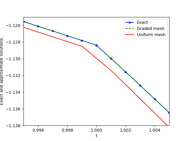
Figure 1: Plot for the results in Ex. 6.1

Example 6.2

Consider the fractional diffusion equation of the form (1.1)-(1.3) with $a=1,c=0,X=\pi,T=1.$ whose exact solution is given by $y(x,t)=\left(t^{3}+t^{\alpha}\right)\sin(x).$

The tables 2, 3 display the maximum absolute errors (MAE) for this example . It is clear from these tables that the numerical results match the theoretical estimates for graded meshes. A comparison between L1 and HL1 in graded meshes shows that HL1 gives better results. This can also be understood through figure 2( for $M=256=N$ and $\alpha=0.6$). One can observe from this figure that high absolute error occurring at $t=0$ diminishes significantly using the proposed scheme.

Table 2: Maximum absolute errors for example 6.2 using HL1 scheme on uniform mesh

$M=N$	$\alpha=0.4$		$\alpha=0.6$		$\alpha=0.8$
	MAE	EOC	MAE	EOC	MAE	EOC
$2^{5}$	$1.04\times 10^{-2}$		$5.45\times 10^{-3}$		$2.42\times 10^{-3}$
$2^{6}$	$8.69\times 10^{-3}$	$0.26$	$4.14\times 10^{-3}$	$0.40$	$1.58\times 10^{-3}$	$0.61$
$2^{7}$	$7.21\times 10^{-3}$	$0.27$	$3.00\times 10^{-3}$	$0.46$	$9.99\times 10^{-4}$	$0.66$
$2^{8}$	$5.79\times 10^{-3}$	$0.31$	$2.11\times 10^{-3}$	$0.50$	$6.08\times 10^{-4}$	$0.72$
$2^{9}$	$4.59\times 10^{-3}$	$0.34$	$1.45\times 10^{-3}$	$0.54$	$3.61\times 10^{-4}$	$0.75$

Table 3: Maximum absolute errors for example 6.2 using

$M=N$	HL1 scheme with $\beta=(3-\alpha)/\alpha$
	$\alpha=0.4$		$\alpha=0.6$		$\alpha=0.8$
	MAE	EOC	MAE	EOC	MAE	EOC
$2^{6}$	$1.35\times 10^{-3}$		$6.43\times 10^{-4}$		$7.00\times 10^{-4}$
$2^{7}$	$2.24\times 10^{-4}$	$2.59$	$1.36\times 10^{-4}$	$2.24$	$1.60\times 10^{-4}$	$2.13$
$2^{8}$	$3.69\times 10^{-5}$	$2.60$	$2.86\times 10^{-5}$	$2.24$	$3.62\times 10^{-5}$	$2.14$
$2^{9}$	$6.09\times 10^{-6}$	$2.60$	$6.08\times 10^{-6}$	$2.25$	$8.20\times 10^{-6}$	$2.14$
$2^{10}$	$1.11\times 10^{-6}$	$2.60$	$1.31\times 10^{-6}$	$2.25$	$1.86\times 10^{-6}$	$2.14$

L1 scheme with $\beta=(2-\alpha)/\alpha$
$\alpha=0.4$		$\alpha=0.6$		$\alpha=0.8$
MAE	EOC	MAE	EOC	MAE	EOC
$4.14\times 10^{-3}$		$5.12\times 10^{-3}$		$7.98\times 10^{-3}$
$1.45\times 10^{-3}$	$1.51$	$1.98\times 10^{-3}$	$1.37$	$3.47\times 10^{-3}$	$1.20$
$5.01\times 10^{-4}$	$1.54$	$7.60\times 10^{-4}$	$1.38$	$1.51\times 10^{-3}$	$1.20$
$1.70\times 10^{-4}$	$1.55$	$2.90\times 10^{-4}$	$1.39$	$6.56\times 10^{-4}$	$1.20$
$5.75\times 10^{-5}$	$1.56$	$1.11\times 10^{-4}$	$1.39$	$2.85\times 10^{-4}$	$1.20$

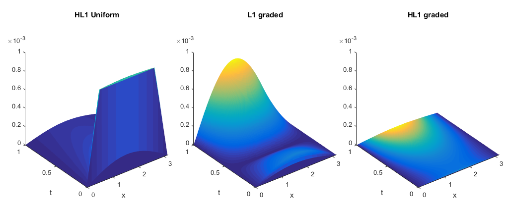
Figure 2: Absolute point-wise error plots for example 6.2

Example 6.3

Consider the following nonlinear TFPDE [10]

$${}_{0}^{C}D_{t}^{\alpha}y(x,t)=\dfrac{\partial^{2}y(x,t)}{\partial x^{2}}-y(x,t)\left(1-y(x,t)\right)+f(x,t),x\in(0,1),t>0,$$

with side conditions

$$y(x,0)=1,x\in[0,1];\quad y(0,t)=1,\;y(1,t)=1+\dfrac{t^{\alpha}}{\Gamma\left(1+\alpha\right)}\sin(1),t\geq 0.$$

The source term is evaluated by taking $y(x,t)=1+\dfrac{t^{\alpha}}{\Gamma\left(1+\alpha\right)}\sin(x),$ as an exact solution. Here the nonlinear example is converted into linearized system of equations using Newton’s quasi-linearization method. Table 4 displays the maximum absolute errors for this example at $\alpha=0.4,0.6,0.8$ and it can be seen that the expected order of convergence (EOC) is achieved. This example was discussed to show the applicability of HL1 scheme to nonlinear problems.

Table 4: Maximum absolute errors for example 6.3 using graded mesh with $\beta=(3-\alpha)/\alpha$

$M=N$	$\alpha=0.4$		$\alpha=0.6$		$\alpha=0.8$
	MAE	EOC	MAE	EOC	MAE	EOC
$2^{4}$	$5.28\times 10^{-2}$		$1.05\times 10^{-2}$		$3.47\times 10^{-3}$
$2^{5}$	$9.18\times 10^{-3}$	$2.524$	$2.11\times 10^{-3}$	$2.254$	$9.06\times 10^{-4}$	$1.940$
$2^{6}$	$1.53\times 10^{-3}$	$2.588$	$4.87\times 10^{-4}$	$2.372$	$2.14\times 10^{-4}$	$2.081$
$2^{7}$	$2.52\times 10^{-4}$	$2.598$	$7.73\times 10^{-5}$	$2.395$	$4.86\times 10^{-5}$	$2.139$
$2^{8}$	$4.16\times 10^{-5}$	$2.600$	$1.46\times 10^{-5}$	$2.399$	$1.08\times 10^{-5}$	$2.170$

7 Conclusion

In this article, we presented the HL1 scheme on graded mesh ($\beta$ the mesh ratio) by taking into consideration the initial singularity arising in the time fractional derivative. Stability analysis and truncation error bounds for the proposed scheme are discussed. The scheme using graded mesh has the order of accuracy to be $\min\left\{\beta\alpha,3-\alpha\right\}.$ It is evident from the numerical examples that the graded mesh scheme resolves the singularity with high resolution by attaining the desired order of accuracy.

References

• [1] H. G. Sun, Y. Zhang, D. Baleanu, W. Chen, Y. Q. Chen, A new collection of real world applications of fractional calculus in science and engineering, Commun. Nonlinear Sci. Numer. Simulat. 64, 213-231 (2018).
• [2] T. A. M. Langlands, B. I. Henry, The accuracy and stability of an implicit solution method for the fractional diffusion equation. J. Comput. Phys. 205, 719-736 (2005).
• [3] B. Jin and Z. Zhou, An analysis of Galerkin proper orthogonal decomposition for sub diffusion, ESAIM Math. Model. Numer. Anal., 51,89-113 (2017).
• [4] G. Naga Raju, H. Madduri: Higher order numerical schemes for the solution of fractional delay differential equations, J. Comput. Appl. Math. DOI: 10.1016/j.cam.2021.113810 (2021).
• [5] M. Stynes, E. O’ Riorden, J. L. Gracia, Error analysis of a finite difference method on graded meshes for a time fractional diffusion equation, SIAM J. Numer. Anal. 55 (2), 1057-1079 (2017).
• [6] J. Ren, C. Huang, N. An, Direct discontinuous Galerkin method for solving nonlinear time fractional diffusion equation with weak singularity solution, Appl. Math. Lett. 102, 106111 (2020).
• [7] R. Zheng, F. Liu, X. Jiang, A Legendre spectral method on graded meshes for the two-dimensional multi-term time-fractional diffusion equation with non-smooth solutions, Appl. Math. Lett. 104, 106247 (2020).
• [8] Y. Luchko, Initial boundary value problems for the one-dimensional time-fractional diffusion equation, Fract. Calc. Appl. Anal., 15, 141-160 (2012).
• [9] M. L. Morgado, N. J. Ford, P. M. Lima, Analysis and numerical methods for fractional differential equations with delay. J. Comput. Appl. Math. 252, 159-168 (2013).
• [10] V. K. Baranwal, R. K. Pandey, M. P. Tripathi, O. P. Singh, An analytic algorithm for time fractional nonlinear reaction–diffusion equation based on a new iterative method. Commun. Nonlinear Sci. Numer. Simulat. 17, 3906-3921 (2012).