New evidence and analysis of cosmological-scale asymmetry in galaxy spin directions

Abstract

In the past several decades, multiple cosmological theories that are based on the contention that the Universe has a major axis have been proposed. Such theories can be based on the geometry of the Universe, or multiverse theories such as black hole cosmology. The contention of a cosmological-scale axis is supported by certain evidence such as the dipole axis formed by the CMB distribution. Here I study another form of cosmological-scale axis, based on the distribution of the spin direction of spiral galaxies. Data from four different telescopes is analyzed, showing nearly identical axis profiles when the distribution of the redshifts of the galaxies is similar.

lshamir@mtu.edu

1 January 20151 January 2015

12.3456/s78910-011-012-3 #### 000 0000 1– 1

1 Introduction

While the Cosmological Principle has been the common working assumption for most cosmological theories, accumulating evidence suggest that the Universe is not necessarily isotropic. Probes that show cosmological-scale anisotropy include the cosmic microwave background (Eriksen et al.,, 2004; Cline et al.,, 2003; Gordon and Hu,, 2004; Campanelli et al.,, 2007; Zhe et al.,, 2015), short gamma ray bursts (Mészáros,, 2019), radio sources (Ghosh et al.,, 2016; Tiwari and Jain,, 2015; Tiwari and Nusser,, 2016), LX-T scaling (Migkas et al.,, 2020), Ia supernova (Javanmardi et al.,, 2015; Lin et al.,, 2016), galaxy morphology types (Javanmardi and Kroupa,, 2017), dark energy (Adhav et al.,, 2011; Adhav,, 2011; Perivolaropoulos,, 2014; Colin et al.,, 2019), polarization of quasars (Hutsemékers et al.,, 2005; Secrest et al.,, 2021), and high-energy cosmic rays (Aab et al.,, 2017).

In particular, the anisotropy of the CMB shows certain evidence of an axis of a cosmological scale (Abramo et al.,, 2006; Mariano and Perivolaropoulos,, 2013; Land and Magueijo,, 2005; Ade et al.,, 2014; Santos et al.,, 2015; Dong et al.,, 2015; Gruppuso et al.,, 2018). A Hubble-scale axis has been also proposed by the anisotropy in cosmological acceleration rates (Perivolaropoulos,, 2014).

These observations can be viewed as a shift from the standard cosmological models (Pecker,, 1997; Perivolaropoulos,, 2014; Bull et al.,, 2016; Velten and Gomes,, 2020). Possible explanations include double inflation (Feng and Zhang,, 2003), contraction prior to inflation (Piao et al.,, 2004), primordial anisotropic vacuum pressure (Rodrigues,, 2008), moving dark energy (Beltran Jimenez and Maroto,, 2007), multiple vacua (Piao,, 2005), or spinor-driven inflation (Bohmer and Mota,, 2008). Other theories can be based on the geometry of the Universe, such as ellipsoidal universe (Campanelli et al.,, 2006, 2007, 2011; Gruppuso,, 2007; Cea,, 2014), geometric inflation (Arciniega et al., 2020a, ; Edelstein et al.,, 2020; Arciniega et al., 2020b, ; Jaime,, 2021), or supersymmetric flows (Rajpoot and Vacaru,, 2017). A cosmological-scale axis is also related to the theory of rotating universe. While early rotating universe theories were based on a static universe (Gödel,, 1949), more recent theories are based on an expanding universe (Ozsváth and Schücking,, 1962; Ozsvath and Schücking,, 2001; Sivaram and Arun,, 2012; Chechin,, 2016; Seshavatharam and Lakshminarayana, 2020a, ; Campanelli,, 2021). In these models, a cosmological-scale axis is expected.

The existence of a cosmological-scale axis can also be linked to holographic big bang (Pourhasan et al.,, 2014; Altamirano et al.,, 2017), and black hole cosmology (Pathria,, 1972; Easson and Brandenberger,, 2001; Chakrabarty et al.,, 2020). These theories can explain cosmic inflation without the assumption of dark energy. Black holes spin (Gammie et al.,, 2004; Mudambi et al.,, 2020; Reynolds,, 2021), and the spin of a black hole is inherited from the spin of the star from which it was created (McClintock et al.,, 2006). If the Universe was formed in a black hole, and the black hole spins, the Universe should have a preferred direction inherited from the spin direction of the black hole (Popławski,, 2010; Seshavatharam,, 2010; Seshavatharam and Lakshminarayana, 2020b, ), leading to an axis (Seshavatharam and Lakshminarayana, 2020a, ). Such black hole universe might not be aligned with the cosmological principle (Stuckey,, 1994). It has also been shown that holography can impact the entropy of a hierarchy of the large-scale structure (Sivaram and Arun,, 2013).

This paper analyzes the possibility of a cosmological-scale axis as predicted by some of these models. A spiral galaxy is an extra-galactic object that its visual appearance changes based on the perspective of the observer. The spin directions of galaxies are aligned within cosmic web filaments (Kraljic et al.,, 2021), and alignment in the spin directions of spiral galaxies have been observed among galaxies that are too far from each other to have gravitational interaction (Lee et al., 2019a, ; Lee et al., 2019b, ). Other studies suggested a correlation between the cosmic initial conditions and the spin direction of spiral galaxies, proposing the contention that galaxy spin direction can be used as a probe to study the early Universe (Motloch et al.,, 2021).

The correlation between the location of spiral galaxies and their spin direction cannot be explained by gravity in its standard form, and was therefore defined as “mysterious” (Lee et al., 2019b, ). Evidence of non-random distribution has been proposed by numerous previous studies (Longo,, 2007, 2011; Shamir,, 2012, 2013, 2016; Shamir, 2017b, ; Shamir, 2017c, ; Shamir, 2017a, ; Shamir,, 2019; Shamir, 2020a, ; Shamir, 2020c, ; Shamir, 2020b, ; Lee et al., 2019a, ; Lee et al., 2019b, ; Shamir, 2021a, ; Shamir, 2021b, ). These observations include several different telescopes such as the Sloan Digial Sky Survey (Shamir,, 2012; Shamir, 2020c, ; Shamir, 2021a, ), the Panoramic Survey Telescope and Rapid Response System (Shamir, 2020c, ), the Hubble Space Telescope (Shamir, 2020a, ), and the Dark Energy Camera (Shamir, 2021b, ). The different telescopes show very similar patterns regardless of the telescope being used, and regardless of whether the galaxies images were analyzed manually or automatically (Shamir, 2021b, ).

This study is based on data from four different telescopes – the Panoramic Survey Telescope and Rapid Response System (PAN-STARRS), the Dark Energy Camera (DECam), the Sloan Digial Sky Survey (SDSS), and the Hubble Space Telescope (HST). The SDSS galaxies also have redshift, which allows to study whether the location of the most likely axis changes with the redshift. Dependence between the location of the most likely axis and the redshift might indicate that the axis, if exists, does not necessarily go through Earth.

2 Galaxy data

The primary dataset used in this study is a dataset of spectroscopic objects identified as galaxies from SDSS. However, to test the consistency of the observations across different telescopes, data from three other telescopes was also used. These telescope include Pan-STARRS, DECam, and HST.

2.1 SDSS data

The SDSS galaxies were taken from (Shamir, 2020c, ). The dataset includes 63,693 galaxies classified with the Ganalyzer algorithm as discussed in Section 2.6. The unique feature of the dataset is that all galaxies have spectra, taken from SDSS DR14. Figure 1 shows the redshift and g magnitude distribution of the objects in the dataset. Figure 2 shows the distribution of the galaxy population in different RA ranges. The full details about the dataset are available in (Shamir, 2020c, ).

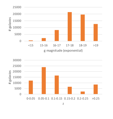
Figure 1: Redshift and g magnitude distribution of the SDSS galaxies. All galaxies have spectra.

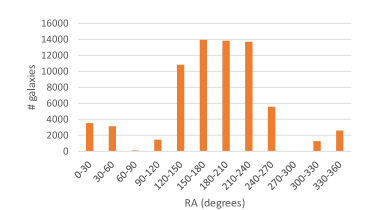
Figure 2: Distribution of the SDSS galaxies across different RA ranges.

2.2 DECam data

The dark energy camera (DECam) of the Blanco 4 meter telescope (Diehl et al.,, 2012; Flaugher et al.,, 2015) covers $\sim 9\cdot 10^{3}$ deg², mostly from the Southern hemisphere. The DECam image data was retrieved through the DESI Legacy Survey API (Dey et al.,, 2019). The description of the dataset and the way it was acquired and annotated is provided in (Shamir, 2021b, ).

In summary, the initial list of objects was taken from Data Release 8 of the DESI Legacy Survey, and included all objects imaged by DECam identified as galaxies, and had magnitude of 19.5 or less in either the g, r or z band. A set of 22,987,246 objects met these criteria. The images of these objects were downloaded by using the cutout service of the DESI Legacy Survey. Each image is a 256$\times$256 JPEG image, and the Petrosian radius was used to scale the image so that the object fits in the frame. All images were downloaded by the exact same computer, to avoid any differences in the way the files were handled by the system. Downloading such a high number of galaxies naturally required nine months, from June 4th 2020 to March 4th, 2021. The data is described in (Shamir, 2021b, ).

As also discussed in Section 2.6, most galaxies are not spiral galaxies or do not have an identifiable spin direction. Therefore, most galaxies were rejected from the analysis and were not assigned with a spin direction. That left a set of 836,451 galaxies in the dataset that were assigned with identifiable spin direction. Some of these galaxies are close satellite galaxies or other large extended objects inside a larger galaxy. To remove such objects, objects that had another object within less than 0.01^o were removed. After removing neighboring objects, 807,898 galaxies were left in the dataset. More information about that dataset is provided in (Shamir, 2021b, ).

Table 1 shows the RA distribution of the DECam galaxies. The DECam galaxies do not have redshift, and therefore the distribution of the redshift was determined by using a subset of 17,027 galaxies that are also included in 2dF (Cole et al.,, 2005). Table 2 shows the redshift distribution of the DECam galaxies.

RA	# galaxies
(degrees)
0-30	155,628
30-60	133,683
60-90	80,134
90-120	21,086
120-150	52,842
150-180	59,660
180-210	58,899
210-240	58,112
240-270	36,490
270-300	2,602
300-330	64,869
330-360	83,893

Table 1: The number of DECam galaxies in different 30^o RA slices.

z	# galaxies
0-0.05	2,089
0.05-0.1	5,487
0.1-0.15	4,226
0.15 - 0.2	1,927
0.2-0.25	784
0.25 - 0.3	621
$>$0.3	1,893

Table 2: The number of DECam galaxies in different redshift ranges. The distribution is determined by a subset of 17,027 galaxies included in the 2dF data release.

2.3 Pan-STARRS data

Pan-STARRS data includes 33,028 galaxies from Pan-STARRS DR1 (Shamir, 2020c, ). The initial set included 2,394,452 Pan-STARRS objects identified as extended sources by all color bands, and g magnitude brighter than 19 (Timmis and Shamir,, 2017). These galaxies were annotated automatically as described in Section 2.6. Most objects in the initial list are too small to allow the identification of their morphology, and therefore just 33,028 with identifiable spin patterns were included in the final dataset.

Figure 3 shows the distribution of Pan-STARRS galaxies. Since Pan-STARRS galaxies do not have redshift, the distribution was determined by a subset of 12,186 galaxies that had redshift through SDSS.

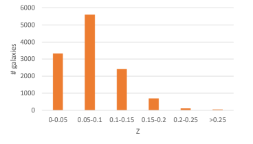
Figure 3: The redshift distribution of 12,186 Pan-STARRS galaxies with spectra in SDSS.

2.4 HST data

While HST cannot provide a dataset of galaxies comparable in size to any of the other digital sky surveys, it has two primary advantages. First of all, the images are not impacted by an atmospheric effect. Although there is no atmospheric effect that can make a galaxy seem to spin in the opposite way, space-based observations can ensure that no unknown atmospheric effect can impact the data. The other advantage is the far deeper field that HST can provide compared to the Earth-based telescope. Because the asymmetry can change with the redshift, using the much more distant HST galaxies can provide information that cannot be provided by the ground-based digital sky surveys.

The dataset of HST galaxies is based on the Hubble Space Telescope (HST) Cosmic Assembly Near-infrared Deep Extragalactic Legacy Survey (Grogin et al.,, 2011; Koekemoer et al.,, 2011). The dataset and the annotation of the galaxies is described in detail in (Shamir, 2020a, ).

The dataset was taken from several fields: the Cosmic Evolution Survey (COSMOS), the Great Observatories Origins Deep Survey North (GOODS-N), the Great Observatories Origins Deep Survey South (GOODS-S), the Ultra Deep Survey (UDS), and the Extended Groth Strip (EGS). The initial set included 114,529 galaxies (Shamir, 2020a, ). The image of each galaxy was extracted by using mSubimage tool (Berriman et al.,, 2004), and converted into 122$\times$122 TIF (Tagged Image File) image format.

Unlike the galaxies of the other telescopes, the HST galaxies were classified by their spin direction manually through a long labor-intensive process. During that process, a random half of the images were mirrored for the first cycle of annotation, and then all images were mirrored for a second cycle of annotation as described in (Shamir, 2020a, ) to offset a possible perceptional bias. That process led to a clean dataset of 8,690 galaxies (Shamir, 2020a, ). Naturally, the HST galaxies are more distant than the galaxies imaged by the other telescopes. Figure 4 shows a histogram of the distribution of the photometric redshift of the HST galaxies. The photometric redshift is highly inaccurate, but even when considering the expected inaccuracy of the photometric redshift it can be safely assumed that the HST galaxies are more distant from Earth compared to the galaxies imaged by the ground-based telescopes. Table 3 shows the number of galaxies taken from each field.

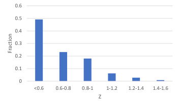
Figure 4: The distribution of the photometric redshift of HST galaxies, as a fraction of the total number in each redshift range.

Table 3: The number of galaxies in each of the five HST fields.

Field	Field	# galaxies	Annotated
	center		galaxies
COSMOS	$150.12^{o},2.2^{o}$	84,424	6,081
GOODS-N	$189.23^{o},62.24^{o}$	5,931	769
GOODS-S	$53.12^{o},-27.81^{o}$	5,024	540
UDS	$214.82^{o},52.82^{o}$	14,245	616
EGS	$34.41^{o},-5.2^{o}$	4,905	684

2.5 Distribution of the galaxy population

The HST galaxies are concentrated in five relatively small fields, making the distribution of these galaxies simple. The other sky surveys cover far larger footprints. Although the footprints are large, they cover merely part of the sky. Moreover, the density of the galaxy population within the footprint of each sky survey is not uniform. Table 1 shows the distribution of the galaxies in different RA ranges in DECam, and Figure 2 displays the distribution of the galaxy population in SDSS, showing that the distribution is not uniform.

Figure 5 shows the galaxy population density in each part of the sky in each of the ground-based telescopes. The distribution is determined by the number of galaxies in each $5^{o}\times 5^{o}$ field of the sky. To avoid bias due to the different surface area covered by pixels closer to the celestial poles, the Hierarchical Equal Area isoLatitude Pixelization (HEALpix) was used. That analysis shows the differences in the density of galaxies in different parts of the sky and in different telescopes. As expected, the different sky surveys have different footprints, and different galaxy distribution within their footprints.

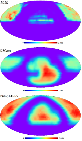
Figure 5: The density of the galaxy population in SDSS, Pan-STARRS and DECam. The galaxy population density in each $5^{o}\times 5^{o}$ field of the sky is determined by the number of galaxies in that $5^{o}\times 5^{o}$ field divided by the total number of galaxies from that telescope.

The different telescopes are not different just in the parts of the sky they cover, but also in the redshift of the galaxies they can image. Obviously, the space-based HST is far deeper than any existing ground-based telescope, and the redshift distribution as shown in Figure 4 is not comparable to any of the ground-based telescopes. The redshift distribution of the three other telescopes is shown in Figure 6.

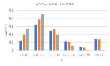
Figure 6: The distribution of the redshift in SDSS, DECam, and Pan-STARRS.

2.6 Galaxy annotation

The HST galaxies were annotated manually, as explained in Section 2.4 and in (Shamir, 2020a, ). The other datasets were far too large to analyze manually, and therefore automatic analysis was needed.

In the recent years, pattern recognition, and especially deep convolutional neural networks (DCNNs), have been becoming very common in classification of galaxy images (Sharma and Baral,, 2018; Ćiprijanović et al.,, 2020). While DCNNs are powerful tools that provide strong classification accuracy for supervised machine learning tasks, they are based on non-intuitive data-driven rules that are difficult to conceptualize. Because these rules are complex and non-intuitive, it is very difficult to ensure their symmetricity. Even a seemingly unimportant aspect such as the order of the training images can lead to a different DCNN and impact the way it works. As shown in (Shamir, 2021a, ), even subtle bias in the classification algorithm can lead to very strong asymmetry in the analysis. Since the asymmetry or other biases in DCNNs are difficult to control or profile, these algorithms are not suitable for identifying subtle asymmetries.

To analyze the galaxy images in a controlled and fully symmetric annotation, the Ganalyzer algorithm was used (Shamir,, 2011). Ganalyzer is not based on any aspect of machine learning, deep learning, or pattern recognition. Instead, it is a model-driven algorithm that follows mathematically defined rules. Ganalyzer first transforms each galaxy image into its radial intensity plot, which is a 360$\times$35 image that reflects the changes of pixel intensity relative to the center of the image. Each pixel $(x,y)$ in the radial intensity plot is the median value of the 5$\times$5 pixels around coordinates $(O_{x}+\sin(\theta)\cdot r,O_{y}-\cos(\theta)\cdot r)$ in the original galaxy image, where r is the radial distance measured in percent of the galaxy radius, $\theta$ is the polar angle, and $(O_{x},O_{y})$ are the pixel coordinates of the center of the galaxy.

Pixels on the galaxy arms are expected to be brighter than pixels that are not on the arm of the galaxy at the same radial distance from the galaxy center. Therefore, peaks in the radial intensity plot are expected to correspond to pixels on the arms of the galaxy at different distances from the galaxy center. A peak detection algorithm (Morháč et al.,, 2000) applied to the lines in the radial intensity plot allows to identify the peaks. Linear regression is then applied to the peaks in adjunct lines. The slope of the lines formed by the peaks reflects the curves of the arms, and consequently the spin direction of the galaxy.

Figure 7 shows examples of galaxy images, their radial intensity plots, and the peaks identified in the radial intensity plots. As the figure shows, each arm is reflected by a vertical line of peaks. The slope of that line indicates the curve of the arms, and consequently the spin directions of the galaxies. More information about Ganalyzer and detailed performance analysis can be found in (Shamir,, 2011; Dojcsak and Shamir,, 2014; Shamir, 2017c, ; Shamir, 2017a, ; Shamir, 2017b, ; Shamir,, 2019; Shamir, 2020c, ; Shamir, 2021b, ).

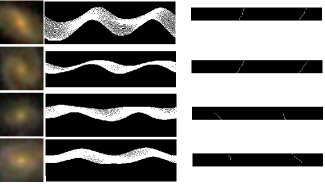
Figure 7: Galaxy images, their radial intensity plots, and the peaks of the radial intensity plots of four different SDSS galaxies.

Since not all galaxies are spiral galaxies, and since not all spiral galaxies have an identifiable spin direction, it is clear that the majority of the galaxies cannot be used for the analysis. Therefore, only galaxies that have at least 30 identified peaks in the radial intensity plot aligned at the same direction are used. Galaxies that do not meet that criterion are rejected regardless of the sign of the linear regression of their peaks. As mentioned above, the primary feature of the algorithm is that it is fully symmetric, and works by clear defined rules.

3 Analysis method

A dipole axis in the distribution of spin directions of galaxies means that the number of spiral galaxies spinning clockwise is higher than the number of galaxies spinning counterclockwise in one hemisphere, but lower in the opposite hemisphere. A simple method is to separate the sky into two hemispheres, and count the number of clockwise and counterclockwise galaxies in each part of the sky. A simple binomial distribution can then provide the statistical significance of the asymmetry.

The advantage of the method is that it is simple, and allows a straightforward statistical analysis. An inverse asymmetry in the two opposite hemispheres indicates on possible asymmetry, but also shows that the asymmetry cannot be driven by a bias in the annotation, as such bias is expected to be consistent throughout the entire sky. That will be discussed thoroughly in Section 5 The downside of this approach is that none of the sky surveys covers the entire sky. Also, the density of the population of the galaxies imaged by each sky survey changes in different parts of the sky, and is not consistent or equally distributed. Ground-based sky surveys can only cover one hemisphere, but in practice cover just a portion of the hemisphere they can observe. That can naturally lead to substantial inconsistencies between different telescopes, as different sky surveys that cover different parts of the sky.

To analyze a dipole axis in a manner that can handle different parts of the sky, a possible axis in the galaxy spin directions of the galaxies can be determined by applying $\chi^{2}$ statistics to fit the spin direction distribution to cosine dependence, as was done in (Shamir,, 2012, 2019; Shamir, 2020a, ; Shamir, 2020c, ). From each possible $(\alpha,\delta)$ combination in the sky, the angular distance $\phi_{i}$ between $(\alpha,\delta)$ and each galaxy i in the dataset was computed. The $\chi^{2}$ from each $(\alpha,\delta)$ was determined by Equation 1

$$\chi^{2}_{\alpha,\delta}=\Sigma_{i}\frac{(d_{i}\cdot|\cos(\phi_{i})|-\cos(\phi_{i}))^{2}}{\cos(\phi_{i})},$$ (1)

where $d_{i}$ is the spin direction of galaxy i such that $d_{i}$ is 1 if the galaxy i spins clockwise, and -1 if the galaxy i spins counterclockwise.

The $\chi^{2}$ is computed using the actual spin directions of the galaxies. Then, the $\chi^{2}$ computed with the actual spin directions is compared to the average $\chi^{2}$ computed in $10^{3}$ runs such that $d_{i}$ of each galaxy i is assigned with a random number within {-1,1}. The standard deviation of the $\chi^{2}$ of the $10^{3}$ runs is also computed. Then, the $\sigma$ difference between the $\chi^{2}$ computed with the actual spin directions and the $\chi^{2}$ computed with the random spin directions provided the probability to have a dipole axis in that $(\alpha,\delta)$ combination by chance.

Repeating that process from each possible $(\alpha,\delta)$ provides a full map of likelihood to have a dipole axis at each point in the sky. Mollweide projection is then used with the Matplotlib library to visualize the results. As will be discussed in Section 5, the measurement used in this study is a relative measurement rather than an absolute measurement. That is, the measurement is not based on differences in the number of galaxies in different parts of the sky. Instead, the measurement is based on the ratio between galaxies with opposite spin directions. Because the number of galaxies spinning clockwise in any field is expected to be within the same order of magnitude of the number of galaxies spinning counterclockwise, non-uniform distribution of the number of galaxies in the sky cannot lead to signal unless the ratio between clockwise and counterclockwise galaxies is indeed statistically different than 1:1. Detailed explanation and experimental results are described in Section 5.1.

Since the analysis attempts to find the best fit into cosine dependence, and since the measurement is relative and not absolute, it is not dependent on the part of the sky being covered, or on the distribution of the galaxy population in the dataset. Because the measurement is relative and not absolute, it is also allows to avoid the assumption of uniform sky coverage, as done in analysis of probes such as CMB. For instance, the obstruction of the Milky Way is expected to affect the number of clockwise galaxies in the same way it affects the number counterclockwise galaxies in the potentially obstructed field, and therefore the effect on both types of galaxies is offset. The analysis method is also described in (Shamir,, 2012, 2019; Shamir, 2020a, ; Shamir, 2020c, ; Shamir, 2021a, ).

4 Results

As a very simple first experiment, the sky was divided into two simple hemispheres by the RA. The first hemisphere was the RA range of $(0^{o}-180^{o})$, and opposite hemisphere $(180^{o}-360^{o})$. The number of galaxies spinning clockwise and the number of galaxies spinning counterclockwise can be compared. Tables 4 and 5 show the number of galaxies spinning clockwise and counterclockwise in the two hemispheres in DECam and SDSS, respectively.

As Table 4 shows, DECam have an excessive number of galaxies spinning clockwise in the $(0^{o}-180^{o})$ hemisphere, and more galaxies spinning counterclockwise in the opposite $(180^{o}-360^{o})$ hemisphere. In both cases the differences are statistically significant. DECam mostly covers the Southern hemisphere. In SDSS, which covers mostly the Northern hemisphere, the asymmetry is inverse. In SDSS a higher number counterclockwise galaxies is observed in the $(0^{o}-180^{o})$ hemisphere, and more clockwise galaxies in the opposite hemisphere. These differences are also statistically significant according to binomial distribution when assuming that the probability of a galaxy to spin clockwise or counterclockwise is 0.5.

Hemisphere	# cw	# ccw	$\frac{cw-ccw}{cw+ccw}$	P
	galaxies	galaxies
$(0^{o}-180^{o})$	252,478	250,555	0.0038	0.0033
$(180^{o}-360^{o})$	151,948	152,917	-0.0033	0.039

Table 4: Number of clockwise and counterclockwise galaxies in opposite hemispheres in DECam. The P values are the binomial distribution probability to have such difference or stronger by chance when assuming 0.5 probability for a galaxy to spin clockwise or counterclockwise.

Hemisphere	# cw	# ccw	$\frac{cw-ccw}{cw+ccw}$	P
	galaxies	galaxies
$(0^{o}-180^{o})$	14,403	15,101	-0.024	0.00002
$(180^{o}-360^{o})$	17,263	16,926	0.01	0.035

Table 5: Number of clockwise and counterclockwise galaxies in opposite hemispheres in SDSS.

While the separation of the sky into two hemispheres is very simple, it relies on a basic and straightforward statistical analysis. To better profile the existence of a dipole axis in the distribution of spin directions of spiral galaxies, the method described in Section 3 was applied. Figure 8 shows a Mollweide projection of the probability of a dipole axis in each integer $(\alpha,\delta)$ combination in the datasets acquired from SDSS, Pan-STARRS, and DECam as described in Section 2.

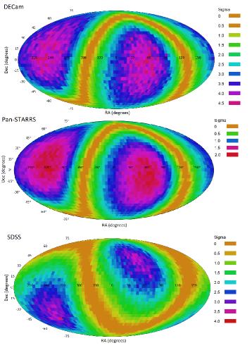
Figure 8: Mollweide projection of the probability of a dipole axis in galaxy spin directions from different $(\alpha,\delta)$ combinations in SDSS, Pan-STARRS, and DECam.

As the figure shows, DECam and Pan-STARRS show a nearly identical profile of asymmetry. The most likely axis in DECam data is identified at $(\alpha=57^{+35^{o}}_{-35^{o}},\delta=-10^{+66^{o}}_{-29^{o}})$, with statistical signal of $4.66\sigma$ (Shamir, 2021b, ). That axis is very close to the most likely axis identified with the Pan-STARRS data, at $(\alpha=47^{o},\delta=-1^{o})$, with statistical significance of 1.87$\sigma$ (Shamir, 2020c, ). It is interesting that the axis is close to the CMB cold spot at $(\alpha=49,\delta=-19^{o})$.

When assigning the galaxies with random spin directions, the signal is immediately lost (Shamir, 2021a, ), and no profile can be identified in any of the telescopes (Shamir, 2020c, ; Shamir, 2021b, ). For instance, Figure 9 shows the profile of asymmetry in the DECam galaxies such that each galaxy was assigned with a random spin direction. A more detailed analysis of “sanity tests” will be discussed in Section 5.

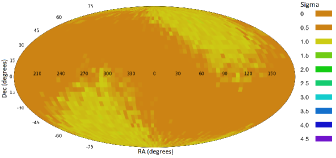
Figure 9: The probability of a dipole axis in galaxy spin directions in DECam data such that the galaxies are assigned with random spin directions.

The analysis done with the SDSS galaxies shows an axis that is close but not identical to DECam and Pan-STARRS. The axis peaks at $(\alpha=69^{+38^{o}}_{-50^{o}},\delta=56^{+21^{o}}_{-31^{o}})$, with statistical significance of 4.63$\sigma$. While that axis is not identical to the axis identified with the DECam data, it is still within 1$\sigma$ from it. While the axes are still within 1$\sigma$ from each other, the SDSS galaxies have different redshift distribution compared to DECam. For instance, 14.7% of the DECam galaxies have redshift greater than 0.25, while in SDSS just 13.5% of the galaxies are in the redshift range. To make a better comparison between the sky surveys, the SDSS galaxy dataset was reduced to a dataset of 38,264 such that the distribution of the redshifts of the galaxies fits the distribution of the redshift of the DECam galaxies. Since all SDSS galaxies have redshift, the normalization of the dataset was done by adding galaxies into the different redshift bins in random order, and excluding a galaxy if the fraction of the galaxies out of the total number of galaxies in its redshift bin is greater than the fraction of that bin in the DECam galaxies. That process leads to a dataset that might be smaller than the original dataset, but its redshift distribution is similar to the dataset it is compared with. Obviously, the process is only possible in datasets were all galaxies have spectra. More information about that process is provided in (Shamir, 2020c, ).

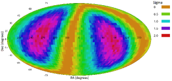
Figure 10: The probability of a dipole axis in galaxy spin directions from different $(\alpha,\delta)$ combinations in SDSS when the redshift distribution is similar to the redshift distribution of the DECam galaxies.

Figure 10 shows the probabilities of a dipole axis from the different $(\alpha,\delta)$ combinations. As the figure shows, when normalizing the distribution of the redshift of the SDSS galaxies, the profile is very similar to the profile of the DECam galaxies. The most likely axis identified in the dataset normalized $(\alpha=78^{o},\delta=-12^{o})$, close to the most likely axis identified in DECam and Pan-STARRS data. In any case, these axes are all within the 1$\sigma$ error, and show good agreement between the different telescopes.

4.1 Analyzing the impact of the redshift distribution

As discussed above, the redshift of the galaxies have an impact on the location of the most likely axis. As a space-based instrument, HST can image deeper objects than the ground-based telescopes. The mean redshift of HST galaxies as approximated by the photometric redshift is 0.58 (Shamir, 2020a, ). Although the photometric redshift is highly inaccurate, it can be safely assumed that the HST galaxies have higher redshift than the SDSS galaxies. The dipole axis formed by HST galaxies was compared to the dipole axis formed by the 15,863 SDSS galaxies with $z>0.15$. Figures 11 shows the probabilities of the axes from each possible integer $(\alpha,\delta)$ combination.

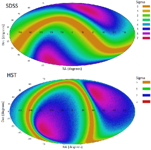
Figure 11: The probability of a dipole axis in galaxy spin directions from different integer $(\alpha,\delta)$ combinations in HST and SDSS when the galaxies are limitied to z$>$0.15.

As the figure shows, when the redshift of the galaxies is high, the axes observed in the two telescopes are in close agreement. The most likely dipole axis identified in the HST galaxies is at $(\alpha=78^{o},\delta=47^{o})$. That is in very close proximity to the most likely dipole axis in the SDSS galaxies with $z>0.15$, peaking at $(\alpha=71^{o},\delta=61^{o})$ as also shown in (Shamir, 2020a, ). The statistical signal of the axis observed with HST galaxies is 2.8$\sigma$, and the SDSS axis probability is 7.4$\sigma$. That difference in the statistical significance can be explained by the fact that the HST galaxies are not distributed in the sky as the SDSS galaxies, but are concentrated in five fields. These five fields might not be located where the asymmetry necessarily peaks. For instance, the most populated HST field is COSMOS, centered around $(\alpha=150^{o},\delta=2^{o})$, where according to the SDSS galaxies the asymmetry exists but does not peak. Table 6 shows the distribution of the galaxies in the COSMOS field of HST, and in the $10^{o}\times 10^{o}$ centered around COSMOS in the other telescopes. All fields show the same direction of the asymmetry, but the asymmetry in the populated fields of HST and DECam is just $\sim$2%.

Sky	# Clockwise	# Counterclockwise	P
survey	galaxies	galaxies	value
COSMOS (HST)	3,116	2,965	0.027
Pan-STARRS	222	190	0.06
SDSS	461	440	0.24
DECam	2,640	2,498	0.025

Table 6: The number of clockwise and counterclockwise galaxies in the HST COSMOS field, and in the $10^{o}\times 10^{o}$ field of SDSS, Pan-STARRS, and DECam centered at COSMOS. The P values are the one-tail binomial probabilities of having asymmetry equal or greater than the observed asymmetry when the probability of a galaxy to spin in a certain direction is 0.5.

4.2 Change of the axis as a function of the redshift

The most likely location of the dipole axis changes with the redshift. That change can be profiled with the SDSS dataset, as all galaxies in that dataset have redshift. For instance, Figure 12 shows the profiles of the asymmetry in several different redshift ranges of $(x<z<x+0.1)$. The figure shows that the location of the most likely axis changes consistently with the redshift. One immediate explanation to the change in the position of the most likely location of the axis with the redshift is that the axis does not necessarily go through Earth.

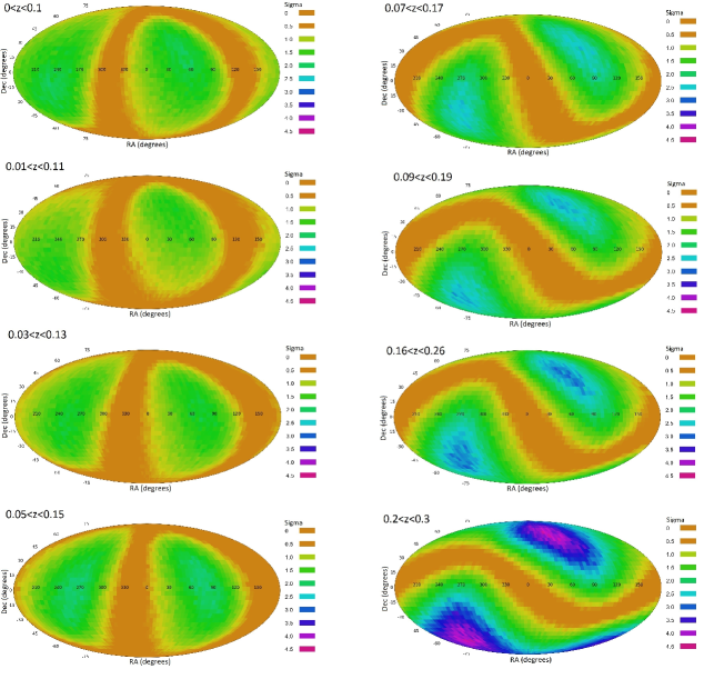
Figure 12: The profile of asymmetry axes in different redshift ranges.

For the analysis, the most likely dipole axis was determined with the SDSS galaxies limited to a 0.1 redshift interval. That was done to all redshift ranges between 0.01$<$z$<$0.11, to 0.16$<$z$<$0.26, where the number of galaxies becomes low. Table 7 show the location of the most likely axis in different redshift ranges. The error of the RA and declination are the low and high 1$\sigma$ error range of the most likely possible axis. Figure 13 displays the change in the RA and declination of the most likely axis in the different redshift ranges. The x-axis shows the mean redshift in each redshift range. Figure 14 shows a similar analysis such that the galaxies are separated into non-overlapping redshift bins. The most distant bin is made of HST galaxies.

z	# galaxies	RA	Dec	$\sigma$
		(degrees)	(degrees)
0.03-0.13	38,938	246$\pm$(56,49)	-20$\pm$(65,33)	1.88
0.04-0.14	38,264	258$\pm$(43,52)	-5$\pm$(61,30)	1.97
0.05-0.15	36,889	266$\pm$(50,45)	8$\pm$(73,28)	2.13
0.06-0.16	34,810	278$\pm$(62,38)	-5$\pm$(44,39)	2.18
0.07-0.17	31,573	270$\pm$(43,33)	-15$\pm$(31,37)	2.42
0.08-0.18	27,500	270$\pm$(52,38)	-21$\pm$(31,21)	2.54
0.09-0.19	23,705	266$\pm$(59,32)	-32$\pm$(23,42)	2.62
0.1-0.2	20,928	269$\pm$(62,29)	-35$\pm$(26,42)	2.50
0.11-0.21	18,018	262$\pm$(51,62)	-38$\pm$(29,40)	2.35
0.12-0.22	14,895	267$\pm$(43,55)	-36$\pm$(30,39)	2.2
0.13-0.23	12,315	265$\pm$(56,45)	-37$\pm$(35,43)	2.4
0.14-0.24	9,957	261$\pm$(63,45)	-40$\pm$(39,39)	2.7
0.15-0.25	8,134	265$\pm$(30,49)	-36$\pm$(46,38)	3.3
0.16-0.26	5,601	267$\pm$(67,32)	-40$\pm$(45,44)	3.2

Table 7: The most likely axis identified in SDSS galaxies when limited to different redshift ranges.

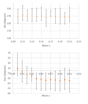
Figure 13: The RA (top) and declination of the most likely axis when the redshift range changes. The error bars show the 1$\sigma$ error of the most likely location of the axis.

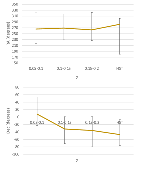
Figure 14: The RA and declination of the most likely axis when the galaxies are separated into non-overlapping redshift bins.

The figures show that the RA of the most likely axis does not change substantially in the examined redshift ranges. The declination, however, changes consistently with the redshift, until it stabilizes at around z$>$0.15. Figure 15 visualizes the most likely axis points in a 3D space such that the distance d is determined by converting the mean redshift of the galaxies in each redshift range to the distance, measured in Mpc. The 3D transformation is then performed simply by Equation LABEL:transformation. As expected, the points are aligned in a manner that forms a 3D axis.

$$x=\cos(\alpha)\cdot d\cdot\cos(\delta)\\ y=\sin(\alpha)\cdot d\cdot\cos(\delta)\\ z=d\cdot sin(\delta)\\$$ (2)

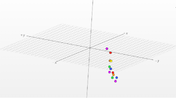
Figure 15: 3D visualization of the points in Table 7.

To approximate the 3D direction of the axis, a simple 3D analysis between two points a and b in a 3D space can be used as shown by Equation LABEL:az_alt_from_3D. The two points from which the direction of the axis was determined are the two most distant points from each other, which are also to two points with the lowest and highest redshift shown in Table 7. The closet point to Earth shown in Table 7 is at $(\alpha=266^{o},\delta=10^{o})$, and 310 Mpc away (z$\simeq$0.07). An observer in that point would see an axis in $(\alpha=268^{o},\delta=-29^{o})$, and the other end of that axis in $(\alpha=88^{o},\delta=29^{o})$.

$$\alpha=atan2(y_{a}-y_{b},\sqrt{(x_{a}-x_{b})^{2}+(z_{a}-z_{b})^{2}})\\ \delta=atan2(-(x_{a}-x_{b}),-(z_{a}-z_{b}))\\$$ (3)

The analysis shown in Table 7 and Figure 12 shows weak signal in $z<0.1$. The $z<0.1$ range might be dominated by galaxies from the local neighborhood, and therefore the presence or absence of alignment of galaxy angular momentum in that redshift range might not provide an observation that can be considered of cosmological scale. Galaxies within clusters are aligned (Tovmassian,, 2021), and galaxies inside the local filament might be aligned in their spin direction (Tempel and Libeskind,, 2013; Pahwa et al.,, 2016; Antipova et al.,, 2021). Therefore a possible cosmological-scale alignment in spin direction might be saturated by alignment inside the Galaxy local neighborhood.

The SDSS galaxies have spectra, and therefore allow to analyze higher redshift range by excluding galaxies with low redshift. That analysis can also be done by using the HST galaxies. Figure 11 shows that both telescopes have similar profiles when the redshift is greater than 0.15. Assuming that $z>0.1$ is considered outside of any local filament, Figure 16 shows the distribution of the spin directions of SDSS galaxies such that $z>0.1$, meaning that all galaxies used are outside of the local neighborhood. The figure shows maximum statistical significance of $\sim 3.2\sigma$ at $(\alpha=49^{+66^{o}}_{-42^{o}},\delta=56^{+28^{o}}_{-34^{o}})$.

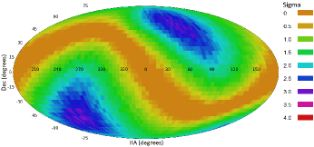
Figure 16: Probability of a dipole axis in different $(\alpha,\delta)$ in SDSS galaxies limited to $z>0.1$.

That provides indication that the signal can be of cosmological scale, and not necessarily a feature of the local neighborhood. The RA of the most likely axis does not change significantly when $z>0.1$, making it difficult to make conclusions about the impact of the change of the RA. The declination changes consistently until $z\simeq 0.15$, where it is stabilizes. The change outside of the local neighborhood might provide a certain indication of cosmological scale axis that does not go directly through Earth, but further research with larger datasets of high-redshift galaxies will be required to study it further. Instruments such as the Dark Energy Spectroscopic Instrument (DESI), when become available, can be combined with optical data such as the DECam data used here to allow further analysis.

Another interesting observation, that can also be seen in Table 7, is that the signal increases as the redshift gets stronger. The observed trend of increasing signal with higher redshift is in agreement with the alignment in the polarization of radio sources, that also gets stronger at higher redshifts (Tiwari and Jain,, 2013).

5 Error analysis and “sanity check”

Naturally, it is important to ensure that the results are not driven by an error. The spin direction of a galaxy is a crude binary variable, and there is no atmospheric or other effect that can flip the spin direction of a galaxy as seen from Earth. While it is difficult to think of an error in the telescope system that can lead to the observation, the fact that four different telescopes show the same profile with a nearly identical profile indicates that it is unlikely that the observation is driven by some unknown error in the telescopes.

Rarely, galaxies can be counter-winding (Grouchy et al.,, 2008), and their actual spin direction is not aligned with the curve of the arms. However, these case are rare, and in any case counter-winding galaxies are equally distributed between galaxies that spin clockwise and galaxies that spin counterclockwise.

The algorithm used for annotating the galaxies (Shamir,, 2011) is fully symmetric. It works by clear and defined rules that are completely symmetric, and the algorithm is not based on pattern recognition, machine learning, or deep learning methods that rely on data-driven non-intuitive rules. Therefore, inaccurate annotation is expected to impact both clockwise and counterclockwise galaxies. That was also tested empirically by mirroring the galaxy images (Shamir, 2021a, ). In all datasets, mirroring the galaxy images led to exactly inverse results (Shamir,, 2012; Shamir, 2020c, ; Shamir, 2020a, ; Shamir, 2021b, ). A more detailed explanation about mirroring the galaxy images is available in (Shamir, 2021a, ).

Also, a bias in the annotation algorithm is expected to lead to similar bias in all parts of the sky, rather than “flip” in opposite hemispheres. The observations in all datasets from all four telescopes show inverse asymmetry in opposite hemispheres. Since each galaxy image is analyzed separately, if a consistent error in the annotation algorithm existed, it would have led to the same asymmetry in all parts of the sky, but not to opposite asymmetry in opposite hemispheres.

If the galaxy annotation algorithm had a certain error in the annotation of the galaxies, the asymmetry A can be defined by Equation 4.

$$A=\frac{(N_{cw}+E_{cw})-(N_{ccw}+E_{ccw})}{N_{cw}+E_{cw}+N_{ccw}+E_{ccw}},$$ (4)

where $E_{cw}$ is the number of Z galaxies incorrectly annotated as S galaxies, and $E_{ccw}$ is the number of S galaxies incorrectly annotated as Z galaxies. Because the algorithm is symmetric, the number of S galaxies incorrectly annotated as Z is expected to be roughly the same as the number of Z galaxies missclassified as S galaxies, and therefore $E_{cw}\simeq E_{ccw}$ (Shamir, 2021a, ). Therefore, the asymmetry A can be defined by Equation 5.

$$A=\frac{N_{cw}-N_{ccw}}{N_{cw}+E_{cw}+N_{ccw}+E_{ccw}}$$ (5)

Since $E_{cw}$ and $E_{ccw}$ cannot be negative, a higher rate of incorrectly annotated galaxies is expected to make A lower. Therefore, when the algorithm is symmetric, incorrect annotation of the galaxies is not expected to lead to asymmetry, and can only make the asymmetry weaker rather than stronger. That has also been tested empirically and showed that error makes the signal weaker rather than stronger, unless the error is asymmetric (Shamir, 2021a, ). For that reason, algorithms that are based on pattern recognition, machine learning, or deep learning cannot be used for this purpose, as they are based on complex data-driven rules that they symmetricity is very difficult to verify.

An empirical experiment (Shamir, 2021a, ) of intentionally annotating some of the galaxies incorrectly showed that even when an error is added, the results do not change significantly even when as many as 25% of the galaxies are assigned with incorrect spin directions, as long as the error is added to both clockwise and counterclockwise galaxies (Shamir, 2021a, ). But if the error is added in an asymmetric manner, even a small asymmetry of 2% leads to a very strong axis that peaks exactly at the celestial pole (Shamir, 2021a, ).

It should be also mentioned that the HST galaxies were annotated manually, with no intervention of any algorithm (Shamir, 2020a, ). Other datasets that were prepared manually were used in (Shamir,, 2016; Shamir, 2017b, ) The asymmetry profile is consistent regardless of the method of annotation, further showing that a computer error is not a likely explanation to the asymmetry.

5.1 Analysis of the distribution of the galaxy population

Obviously, no Earth-based telescope can cover the entire sky, and the footprint of the sky covered by any Earth-based telescope is merely a portion of the entire sky. As discussed in Section 2.5, the galaxies in the sky surveys are not distributed uniformly inside their footprints. Such non-uniform distribution can in some cases lead to a shift in the location of the most likely axis. For instance, Tiwari et al., (2019) showed that the TGSS ADR1 catalog of radio sources might not be suitable for observing large-scale or moderate scale anisotropy also due to non-uniform distribution of the sources throughout the sky.

What makes the probe of spin direction distribution of spiral galaxies different from other probes is that the spin direction is a comparative measurement, rather than an absolute measurement. Absolute measurements such as CMB or the number of radio sources can be impacted by the distribution of the measurements, as well as by other effects such as Milky Way obstruction. For instance, if the Milky Way obstructs some of the sky, the change in the temperature in that part of the sky can lead to certain anisotropy. When counting radio sources, an anisotropy can be driven by differences in the coverage of different parts of the sky Tiwari et al., (2019).

The ratio between galaxies that spin in opposite directions is a comparative scale, meaning that it is not determined by the number of galaxies in a certain field, but by the difference between the number of galaxies spinning clockwise and the number of galaxies spinning counterclockwise in that field. In each given field, the number of clockwise galaxies is balanced by a roughly similar number of counterclockwise galaxies. The cosine dependence analysis described in Section 3 identifies the best axis that fits the distribution of the clockwise and counterclockwise spiral galaxies. Because the measurement is relative, it is expected to be less sensitive to the distribution of the absolute number of galaxies, as each field that used in the analysis has a roughly similar number of galaxies that spin in each direction. Therefore, four different telescopes with four different footprints provide very similar location of the most likely axis.

To test the effect of the non-uniform distribution of the galaxies empirically, the galaxies from the four telescopes were combined into a single dataset. In order not to use the same galaxy more than once, galaxies that appear in two or more telescopes were removed, leading to a dataset of 935,155 galaxies. To create a dataset of galaxies that are distributed uniformly within the footprint, the 935,155 galaxies were added in random order into a new dataset such that before adding a galaxy to the dataset, the number of galaxies with 5^o radius from that galaxy was counted. If 500 or more galaxies are present within a distance of 5^o, the galaxy is not added to the dataset. Otherwise, the galaxy is added. The algorithm for creating that dataset U from the dataset D of 935,155 galaxies can be summarized as follows:

1. U $\leftarrow$ {}
2. For each galaxy d in D
3.       galaxy_counter $\leftarrow$ 0
4.       For each galaxy u in U
5.           if distance(d,u)$<5^{o}$
6.               galaxy_counter $\leftarrow$ galaxy_counter +1
7.       if galaxy_counter$<$500
8.           add galaxy d to U

Then, isolated galaxies in dataset U that do not have 500 galaxies within 5^o are removed from U. When the galaxies in D are iterated in random order, that process leads to a dataset U of 193,368 galaxies that are distributed uniformly inside the combined footprint. Figure 17 shows the distribution of the galaxy population in different parts of the sky. The dataset is smaller than the DECam dataset, but spreads much more uniformly in the sky compared to the other sky surveys. Figure 18 shows the probability for a dipole axis in each $(\alpha,\delta)$ combination. The most likely axis is at $(\alpha=63^{o},delta=-16^{o})$.

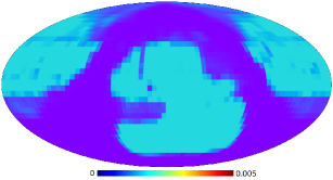
Figure 17: The density of the galaxy population in the combined dataset with uniform distribution of the galaxies inside the combined footprint. The galaxy population density in each point of the sky is determined by the number of galaxies within 5^o from that point, divided by the total number of galaxies.

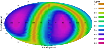
Figure 18: The probability of the most likely axis from each $(\alpha,\delta)$ combinations. The number of galaxies is similar in the different populated parts of the sky.

As the figure shows, when the distribution of the galaxies is uniform, and no certain parts of the sky are overpopulated or underpopulated, the profile of the asymmetry is in agreement with the profile determined by DECam or Pan-STARRS when the galaxy population is not normalized. Considering the ratio in each part of the sky as temperature, the HEALPix library (Zonca et al.,, 2019) can also be used to profile the dipole, showing a dipole at $(\alpha=45^{o},\delta=-23^{o})$.

As mentioned above, there is no Earth-based telescope that can cover the entire sky. Even when combining the footprints of all telescopes, substantial parts of the sky are not covered. The relative measurement used here is expected to lead to the same profile of best cosine fitness regardless of the parts of the sky that are covered, given that the sky coverage is sufficiently large to allow fitness. However, the non-uniform distribution of the parts of the sky that need to be covered should be tested empirically. For that purpose, an experiment was performed such that only two parts of the sky were used, in two exactly opposite hemispheres. The two parts of the sky were $(0^{o}<\alpha<60^{o},-45^{o}<\delta<0^{o})$, and the exact same part of the sky in the opposite hemisphere $(180^{o}<\alpha<240^{o},0^{o}<\delta<45^{o})$. These are two exact opposite parts of the sky, and therefore an asymmetry profile is not expected to be driven by non-uniform distribution of the galaxies in the sky. That dataset included 282,252 galaxies. Figure 19 show the results, with the most likely axis peaking with 5.4$\sigma$ at $(\alpha=41^{o},\delta=-12^{o})$, well within the 1$\sigma$ error of the analysis when using the entire dataset.

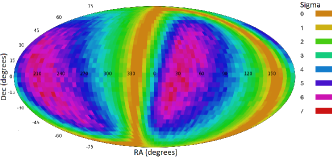
Figure 19: The probability of the most likely axis from each $(\alpha,\delta)$ combinations. The parts of the sky used in the analysis are of similar size in exact opposite hemispheres.

6 Conclusions

Multiple sky surveys have shown certain patterns of asymmetry between clockwise and counterclockwise galaxies. These sky surveys include SDSS (Shamir,, 2012; Shamir, 2020c, ), Pan-STARRS (Shamir, 2020c, ), DECam (Shamir, 2021b, ), and HST (Shamir, 2020a, ). These observations include different ways of annotating the galaxies, observations from both the the Northern and Southern hemispheres, and observations from ground-based and space-based instruments. All observations are in very good agreement. As multiple probes have shown disagreement with the cosmological isotropy assumption, the contention that the Universe is oriented around an axis is in agreement with several existing cosmological theories such as black hole cosmology, elliptodial universe, rotating universe, and other cosmological models that provide an alternative to the standard model.

One of the possible weaknesses of the analysis is that the footprint does not cover the entire sky. As no Earth-based sky survey can cover the entire sky, an experiment that provides 100% sky coverage is not possible. The use of a comparative measurement and not an absolute measurement makes the analysis more robust to cases of non-uniform distribution. Several empirical experiments were also performed to analyze the impact of the asymmetric shape of the footprint, showing consistent results, although no experiment that covers the entire sky can be done, as the sky surveys do not provide full sky coverage.

The observations show that the location of the most likely axis changes with the redshift at $z>0.1$. That can be viewed as an indication that if such axis exists, it does not necessarily go directly through Earth. The general location of the axis at $(\alpha=\sim 260^{o},\delta=\sim-40^{o})$ is roughly aligned with the axis formed by the isotropy of the accelerating cosmological expansion rate at $(\alpha=223^{o},\delta=-76.2^{o})$ as explained in (Perivolaropoulos,, 2014). The Shapely supercluster (Sheth and Diaferio,, 2011) is also not far at $(\alpha=202^{o},\delta=-30^{o})$.

As the evidence of cosmological-scale anisotropy are accumulating, theories that provide alternatives or expansions to the standard cosmology model are being proposed (Arun et al.,, 2017; Nadathur et al.,, 2012; Narlikar et al.,, 2007; Perivolaropoulos,, 2014; Bull et al.,, 2016; López-Corredoira,, 2017; Scott,, 2018; Tatum et al.,, 2018; Neves,, 2020; Nojiri et al.,, 2019; López-Corredoira,, 2017; Freedman,, 2017; Fiscaletti,, 2018; Tatum et al.,, 2018; Guo et al.,, 2019; Li,, 2021). Such cosmological-scale alignment between galaxies can also be related to alternative gravitational theories that shift from the Newtonian model (Bekenstein and Milgrom,, 1984; Milgrom,, 2009; Deser and Tekin,, 2007; Alkaç and Tekin,, 2018; Sivaram et al.,, 2020; Sivaram et al., 2021b, ; Sivaram et al., 2021a, ), where gravity span is far greater than assumed by the existing models of gravity (Amendola et al.,, 2020; Falcon,, 2021). Such gravity models have impact on cosmology (Sivaram,, 1994), and can also explain other anomalies that disagree with the standard model such as the Keenan–Barger–Cowie (KBC) void (Haslbauer et al.,, 2020) and the El Gordo (ACT-CL J0102-4915) massive galaxy cluster (Asencio et al.,, 2020). It is therefore important to continue to explore different probes and different observations that can provide more information about the structure of the Universe. Clearly, further research will be required to fully profile the nature of the asymmetry.

References

- Aab et al., (2017) Aab, A., Abreu, P., Aglietta, M., Al Samarai, I., Albuquerque, I., Allekotte, I., Almela, A., Castillo, J. A., Alvarez-Muñiz, J., Anastasi, G. A., et al. (2017). Observation of a large-scale anisotropy in the arrival directions of cosmic rays above 8 1018 ev. Science, 357(6357):1266–1270.
- Abramo et al., (2006) Abramo, L. R., Sodré Jr, L., and Wuensche, C. A. (2006). Anomalies in the low cmb multipoles and extended foregrounds. Physical Review D, 74(8):083515.
- Ade et al., (2014) Ade, P. A., Aghanim, N., Armitage-Caplan, C., Arnaud, M., Ashdown, M., Atrio-Barandela, F., Aumont, J., Baccigalupi, C., Banday, A. J., Barreiro, R., et al. (2014). Planck 2013 results. xxiii. isotropy and statistics of the cmb. Astronomy & Astrophysics, 571:A23.
- Adhav et al., (2011) Adhav, K., Bansod, A., Wankhade, R., and Ajmire, H. (2011). Kantowski-sachs cosmological models with anisotropic dark energy. Open Physics, 9(4):919–925.
- Adhav, (2011) Adhav, K. S. (2011). Lrs bianchi type-i universe with anisotropic dark energy in lyra geometry. International Journal of Astronomy and Astrophysics, 1(4):204–209.
- Alkaç and Tekin, (2018) Alkaç, G. and Tekin, B. (2018). Holographic c-theorem and born-infeld gravity theories. Physical Review D, 98(4):046013.
- Altamirano et al., (2017) Altamirano, N., Gould, E., Afshordi, N., and Mann, R. B. (2017). Cosmological perturbations in the 5d holographic big bang model. arXiv preprint arXiv:1703.00954.
- Amendola et al., (2020) Amendola, L., Bettoni, D., Pinho, A. M., and Casas, S. (2020). Measuring gravity at cosmological scales. Universe, 6(2):20.
- Antipova et al., (2021) Antipova, A., Makarov, D., and Bizyaev, D. (2021). Orientation of the spins of flat galaxies relative to filaments of a large-scale structure of the universe. Astrophysical Bulletin, 76(3):248–254.
- (10) Arciniega, G., Bueno, P., Cano, P. A., Edelstein, J. D., Hennigar, R. A., and Jaime, L. G. (2020a). Geometric inflation. Physics Letters B, 802:135242.
- (11) Arciniega, G., Edelstein, J. D., and Jaime, L. G. (2020b). Towards geometric inflation: the cubic case. Physics Letters B, 802:135272.
- Arun et al., (2017) Arun, K., Gudennavar, S., and Sivaram, C. (2017). Dark matter, dark energy, and alternate models: A review. Advances in Space Research, 60(1):166–186.
- Asencio et al., (2020) Asencio, E., Banik, I., and Kroupa, P. (2020). A massive blow for cdm- the high redshift, mass, and collision velocity of the interacting galaxy cluster el gordo contradicts concordance cosmology. Monthly Notices of the Royal Astronomical Society, 500(4):5249–5267.
- Bekenstein and Milgrom, (1984) Bekenstein, J. and Milgrom, M. (1984). Does the missing mass problem signal the breakdown of newtonian gravity? The Astrophysical Journal, 286:7–14.
- Beltran Jimenez and Maroto, (2007) Beltran Jimenez, J. and Maroto, A. L. (2007). Cosmology with moving dark energy and the cmb quadrupole. Physical Review D, 76(2):023003.
- Berriman et al., (2004) Berriman, G. B., Good, J. C., Laity, A. C., Bergou, A., Jacob, J., Katz, D. S., Deelman, E., Kesselman, C., Singh, G., Su, M.-H., et al. (2004). Montage: a grid enabled image mosaic service for the national virtual observatory. In Astronomical Data Analysis Software and Systems (ADASS) XIII, volume 314, page 593.
- Bohmer and Mota, (2008) Bohmer, C. G. and Mota, D. F. (2008). Cmb anisotropies and inflation from non-standard spinors. Physics Letters B, 663(3):168–171.
- Bull et al., (2016) Bull, P., Akrami, Y., Adamek, J., Baker, T., Bellini, E., Jimenez, J. B., Bentivegna, E., Camera, S., Clesse, S., Davis, J. H., et al. (2016). Beyond cdm: Problems, solutions, and the road ahead. Physics of the Dark Universe, 12:56–99.
- Campanelli, (2021) Campanelli, L. (2021). A conjecture on the neutrality of matter. Foundations of Physics, 51:56.
- Campanelli et al., (2011) Campanelli, L., Cea, P., Fogli, G., and Tedesco, L. (2011). Cosmic parallax in ellipsoidal universe. Modern Physics Letters A, 26(16):1169–1181.
- Campanelli et al., (2006) Campanelli, L., Cea, P., and Tedesco, L. (2006). Ellipsoidal universe can solve the cosmic microwave background quadrupole problem. Physical Review Letters, 97(13):131302.
- Campanelli et al., (2007) Campanelli, L., Cea, P., and Tedesco, L. (2007). Cosmic microwave background quadrupole and ellipsoidal universe. Physical Review D, 76(6):063007.
- Cea, (2014) Cea, P. (2014). The ellipsoidal universe in the planck satellite era. Monthly Notices of the Royal Astronomical Society, 441(2):1646–1661.
- Chakrabarty et al., (2020) Chakrabarty, H., Abdujabbarov, A., Malafarina, D., and Bambi, C. (2020). A toy model for a baby universe inside a black hole. European Physical Journal C, 80(1909.07129):1–10.
- Chechin, (2016) Chechin, L. (2016). Rotation of the universe at different cosmological epochs. Astronomy Reports, 60(6):535–541.
- Ćiprijanović et al., (2020) Ćiprijanović, A., Snyder, G. F., Nord, B., and Peek, J. E. (2020). Deepmerge: Classifying high-redshift merging galaxies with deep neural networks. Astronomy and Computing, 32:100390.
- Cline et al., (2003) Cline, J. M., Crotty, P., and Lesgourgues, J. (2003). Does the small cmb quadrupole moment suggest new physics? Journal of Cosmology and Astroparticle Physics, 2003(09):010.
- Cole et al., (2005) Cole, S., Percival, W. J., Peacock, J. A., Norberg, P., Baugh, C. M., Frenk, C. S., Baldry, I., Bland-Hawthorn, J., Bridges, T., Cannon, R., et al. (2005). The 2df galaxy redshift survey: power-spectrum analysis of the final data set and cosmological implications. Monthly Notices of the Royal Astronomical Society, 362(2):505–534.
- Colin et al., (2019) Colin, J., Mohayaee, R., Rameez, M., and Sarkar, S. (2019). Evidence for anisotropy of cosmic acceleration. Astronomy & Astrophysics, 631:L13.
- Deser and Tekin, (2007) Deser, S. and Tekin, B. (2007). New energy definition for higher-curvature gravities. Physical Review D, 75(8):084032.
- Dey et al., (2019) Dey, A., Schlegel, D. J., Lang, D., Blum, R., Burleigh, K., Fan, X., Findlay, J. R., Finkbeiner, D., Herrera, D., Juneau, S., et al. (2019). Overview of the desi legacy imaging surveys. Astronomical Journal, 157(5):168.
- Diehl et al., (2012) Diehl, T., Collaboration, D. E. S., et al. (2012). The dark energy survey camera (decam). Physics Procedia, 37:1332–1340.
- Dojcsak and Shamir, (2014) Dojcsak, L. and Shamir, L. (2014). Quantitative analysis of spirality in elliptical galaxies. New Astronomy, 28:1–8.
- Dong et al., (2015) Dong, Z., Ming-Hua, L., Ping, W., and Zhe, C. (2015). Inflation in de sitter spacetime and cmb large scale anomaly. Chinese Physics C, 39(9):095101.
- Easson and Brandenberger, (2001) Easson, D. A. and Brandenberger, R. H. (2001). Universe generation from black hole interiors. Journal of High Energy Physics, 2001(06):024.
- Edelstein et al., (2020) Edelstein, J. D., Rodríguez, D. V., and López, A. V. (2020). Aspects of geometric inflation. Journal of Cosmology and Astroparticle Physics, 2020(12):040.
- Eriksen et al., (2004) Eriksen, H. K., Hansen, F. K., Banday, A. J., Gorski, K. M., and Lilje, P. B. (2004). Asymmetries in the cosmic microwave background anisotropy field. Astrophysical Journal, 605(1):14.
- Falcon, (2021) Falcon, N. (2021). A large-scale heuristic modification of newtonian gravity as alternative approach to the dark energy and dark matter. Journal of Astrophysics and Astronomy, 42(102).
- Feng and Zhang, (2003) Feng, B. and Zhang, X. (2003). Double inflation and the low cmb quadrupole. Physics Letters B, 570(3-4):145–150.
- Fiscaletti, (2018) Fiscaletti, D. (2018). Towards a non-local timeless quantum cosmology for the beyond standard model physics. Bulgarian Journal of Physics, 45(4).
- Flaugher et al., (2015) Flaugher, B., Diehl, H., Honscheid, K., Abbott, T., Alvarez, O., Angstadt, R., Annis, J., Antonik, M., Ballester, O., Beaufore, L., et al. (2015). The dark energy camera. The Astronomical Journal, 150(5):150.
- Freedman, (2017) Freedman, W. L. (2017). Cosmology at a crossroads. Nature Astronomy, 1(5):1–3.
- Gammie et al., (2004) Gammie, C. F., Shapiro, S. L., and McKinney, J. C. (2004). Black hole spin evolution. The Astrophysical Journal, 602(1):312.
- Ghosh et al., (2016) Ghosh, S., Jain, P., Kashyap, G., Kothari, R., Nadkarni-Ghosh, S., and Tiwari, P. (2016). Probing statistical isotropy of cosmological radio sources using square kilometre array. Journal of Astrophysics and Astronomy, 37(4):1–21.
- Gödel, (1949) Gödel, K. (1949). An example of a new type of cosmological solutions of einstein’s field equations of gravitation. Reviews of Modern Physics, 21(3):447.
- Gordon and Hu, (2004) Gordon, C. and Hu, W. (2004). Low cmb quadrupole from dark energy isocurvature perturbations. Physical Review D, 70(8):083003.
- Grogin et al., (2011) Grogin, N. A., Kocevski, D. D., Faber, S., Ferguson, H. C., Koekemoer, A. M., Riess, A. G., Acquaviva, V., Alexander, D. M., Almaini, O., Ashby, M. L., et al. (2011). Candels: the cosmic assembly near-infrared deep extragalactic legacy survey. Astrophysical Journal Supplement Series, 197(2):35.
- Grouchy et al., (2008) Grouchy, R., Buta, R., Salo, H., Laurikainen, E., and Speltincx, T. (2008). Counter-winding spiral structure in eso 297-27. The Astronomical Journal, 136(3):980.
- Gruppuso, (2007) Gruppuso, A. (2007). Complete statistical analysis for the quadrupole amplitude in an ellipsoidal universe. Physical Review D, 76(8):083010.
- Gruppuso et al., (2018) Gruppuso, A., Kitazawa, N., Lattanzi, M., Mandolesi, N., Natoli, P., and Sagnotti, A. (2018). The evens and odds of cmb anomalies. Physics of the Dark Universe, 20:49–64.
- Guo et al., (2019) Guo, R.-Y., Zhang, J.-F., and Zhang, X. (2019). Can the h0 tension be resolved in extensions to cdm cosmology? Journal of Cosmology and Astroparticle Physics, 2019(02):054.
- Haslbauer et al., (2020) Haslbauer, M., Banik, I., and Kroupa, P. (2020). The kbc void and hubble tension contradict cdm on a gpc scale- milgromian dynamics as a possible solution. Monthly Notices of the Royal Astronomical Society, 499(2):2845–2883.
- Hutsemékers et al., (2005) Hutsemékers, D., Cabanac, R., Lamy, H., and Sluse, D. (2005). Mapping extreme-scale alignments of quasar polarization vectors. Astronomy & Astrophysics, 441(3):915–930.
- Jaime, (2021) Jaime, L. G. (2021). On the viability of the evolution of the universe with geometric inflation. Physics of the Dark Universe, page 100887.
- Javanmardi and Kroupa, (2017) Javanmardi, B. and Kroupa, P. (2017). Anisotropy in the all-sky distribution of galaxy morphological types. Astronomy & Astrophysics, 597:A120.
- Javanmardi et al., (2015) Javanmardi, B., Porciani, C., Kroupa, P., and Pflam-Altenburg, J. (2015). Probing the isotropy of cosmic acceleration traced by type ia supernovae. Astrophysical Journal, 810(1):47.
- Koekemoer et al., (2011) Koekemoer, A. M., Faber, S., Ferguson, H. C., Grogin, N. A., Kocevski, D. D., Koo, D. C., Lai, K., Lotz, J. M., Lucas, R. A., McGrath, E. J., et al. (2011). Candels: The cosmic assembly near-infrared deep extragalactic legacy survey—the hubble space telescope observations, imaging data products, and mosaics. Astrophysical Journal Supplement Series, 197(2):36.
- Kraljic et al., (2021) Kraljic, K., Duckworth, C., Tojeiro, R., Alam, S., Bizyaev, D., Weijmans, A.-M., Boardman, N. F., and Lane, R. R. (2021). Sdss-iv manga: 3d spin alignment of spiral and s0 galaxies. Monthly Notices of the Royal Astronomical Society.
- Land and Magueijo, (2005) Land, K. and Magueijo, J. (2005). Examination of evidence for a preferred axis in the cosmic radiation anisotropy. Physical Review Letters, 95(7):071301.
- (60) Lee, J. H., Pak, M., Lee, H.-R., and Song, H. (2019a). Galaxy rotation coherent with the motions of neighbors: Discovery of observational evidence. Astrophysical Journal, 872(1):78.
- (61) Lee, J. H., Pak, M., Song, H., Lee, H.-R., Kim, S., and Jeong, H. (2019b). Mysterious coherence in several-megaparsec scales between galaxy rotation and neighbor motion. Astrophysical Journal, 884(2):104.
- Li, (2021) Li, Z. (2021). Meta-interaction physics between supergravity and dark energy behind super-inflating universe. Journal of Astrophysics and Astronomy, 42(2):1–40.
- Lin et al., (2016) Lin, H.-N., Li, X., and Chang, Z. (2016). The significance of anisotropic signals hiding in the type ia supernovae. Monthly Notices of the Royal Astronomical Society, 460(1):617–626.
- Longo, (2007) Longo, M. J. (2007). Is the cosmic” axis of evil” due to a large-scale magnetic field. arXiv preprint astro-ph/0703694.
- Longo, (2011) Longo, M. J. (2011). Detection of a dipole in the handedness of spiral galaxies with redshifts z 0.04. Physics Letters B, 699(4):224–229.
- López-Corredoira, (2017) López-Corredoira, M. (2017). Tests and problems of the standard model in cosmology. Foundations of Physics, 47(6):711–768.
- Mariano and Perivolaropoulos, (2013) Mariano, A. and Perivolaropoulos, L. (2013). Cmb maximum temperature asymmetry axis: Alignment with other cosmic asymmetries. Physical Review D, 87(4):043511.
- McClintock et al., (2006) McClintock, J. E., Shafee, R., Narayan, R., Remillard, R. A., Davis, S. W., and Li, L.-X. (2006). The spin of the near-extreme kerr black hole grs 1915+ 105. Astrophysical Journal, 652(1):518.
- Mészáros, (2019) Mészáros, A. (2019). An oppositeness in the cosmology: Distribution of the gamma ray bursts and the cosmological principle. Astronomical Notes, 340(7):564–569.
- Migkas et al., (2020) Migkas, K., Schellenberger, G., Reiprich, T., Pacaud, F., Ramos-Ceja, M., and Lovisari, L. (2020). Probing cosmic isotropy with a new x-ray galaxy cluster sample through the lx–t scaling relation. Astronomy & Astrophysics, 636:A15.
- Milgrom, (2009) Milgrom, M. (2009). Bimetric mond gravity. Physical Review D, 80(12):123536.
- Morháč et al., (2000) Morháč, M., Kliman, J., Matoušek, V., Veselskỳ, M., and Turzo, I. (2000). Identification of peaks in multidimensional coincidence -ray spectra. Nuclear Instruments and Methods in Physics Research Section A: Accelerators, Spectrometers, Detectors and Associated Equipment, 443(1):108–125.
- Motloch et al., (2021) Motloch, P., Yu, H.-R., Pen, U.-L., and Xie, Y. (2021). An observed correlation between galaxy spins and initial conditions. Nature Astronomy, 5(3):283–288.
- Mudambi et al., (2020) Mudambi, S. P., Rao, A., Gudennavar, S., Misra, R., and Bubbly, S. (2020). Estimation of the black hole spin in lmc x-1 using astrosat. Monthly Notices of the Royal Astronomical Society, 498(3):4404–4410.
- Nadathur et al., (2012) Nadathur, S., Hotchkiss, S., and Sarkar, S. (2012). The integrated sachs-wolfe imprint of cosmic superstructures: a problem for cdm. Journal of Cosmology and Astroparticle Physics, 2012(06):042.
- Narlikar et al., (2007) Narlikar, J. V., Burbidge, G., and Vishwakarma, R. (2007). Cosmology and cosmogony in a cyclic universe. Journal of Astrophysics and Astronomy, 28(2):67–99.
- Neves, (2020) Neves, J. (2020). Proposal for a degree of scientificity in cosmology. Foundations of Science, 25(3):857–878.
- Nojiri et al., (2019) Nojiri, S., Odintsov, S. D., and Saridakis, E. N. (2019). Modified cosmology from extended entropy with varying exponent. The European Physical Journal C, 79(3):1–10.
- Ozsváth and Schücking, (1962) Ozsváth, I. and Schücking, E. (1962). Finite rotating universe. Nature, 193(4821):1168–1169.
- Ozsvath and Schücking, (2001) Ozsvath, I. and Schücking, E. (2001). Approaches to gödel’s rotating universe. Classical and Quantum Gravity, 18(12):2243.
- Pahwa et al., (2016) Pahwa, I., Libeskind, N. I., Tempel, E., Hoffman, Y., Tully, R. B., Courtois, H. M., Gottlöber, S., Steinmetz, M., and Sorce, J. G. (2016). The alignment of galaxy spin with the shear field in observations. Monthly Notices of the Royal Astronomical Society, 457(1):695–703.
- Pathria, (1972) Pathria, R. (1972). The universe as a black hole. Nature, 240(5379):298–299.
- Pecker, (1997) Pecker, J.-C. (1997). Some critiques of the big bang cosmology. Journal of Astrophysics and Astronomy, 18(4):323–333.
- Perivolaropoulos, (2014) Perivolaropoulos, L. (2014). Large scale cosmological anomalies and inhomogeneous dark energy. Galaxies, 2(1):22–61.
- Piao, (2005) Piao, Y.-S. (2005). Possible explanation to a low cmb quadrupole. Physical Review D, 71(8):087301.
- Piao et al., (2004) Piao, Y.-S., Feng, B., and Zhang, X. (2004). Suppressing the cmb quadrupole with a bounce from the contracting phase to inflation. Physical Review D, 69(10):103520.
- Popławski, (2010) Popławski, N. J. (2010). Cosmology with torsion: An alternative to cosmic inflation. Physics Letters B, 694(3):181–185.
- Pourhasan et al., (2014) Pourhasan, R., Afshordi, N., and Mann, R. B. (2014). Out of the white hole: a holographic origin for the big bang. Journal of Cosmology and Astroparticle Physics, 2014(04):005.
- Rajpoot and Vacaru, (2017) Rajpoot, S. and Vacaru, S. I. (2017). On supersymmetric geometric flows and r2 inflation from scale invariant supergravity. Annals of Physics, 384:20–60.
- Reynolds, (2021) Reynolds, C. S. (2021). Observational constraints on black hole spin. Annual Review of Astronomy and Astrophysics, 59:117–154.
- Rodrigues, (2008) Rodrigues, D. C. (2008). Anisotropic cosmological constant and the cmb quadrupole anomaly. Physical Review D, 77(2):023534.
- Santos et al., (2015) Santos, L., Cabella, P., Villela, T., and Zhao, W. (2015). Influence of planck foreground masks in the large angular scale quadrant cmb asymmetry. Astronomy & Astrophysics, 584:A115.
- Scott, (2018) Scott, D. (2018). The Standard Model of cosmology: A skeptic’s guide.
- Secrest et al., (2021) Secrest, N. J., von Hausegger, S., Rameez, M., Mohayaee, R., Sarkar, S., and Colin, J. (2021). A test of the cosmological principle with quasars. The Astrophysical Journal Letters, 908(2):L51.
- Seshavatharam, (2010) Seshavatharam, U. (2010). Physics of rotating and expanding black hole universe. Progress in Physics, 2:7–14.
- (96) Seshavatharam, U. and Lakshminarayana, S. (2020a). An integrated model of a light speed rotating universe. International Astronomy and Astrophysics Research Journal, pages 74–82.
- (97) Seshavatharam, U. and Lakshminarayana, S. (2020b). Light speed expansion and rotation of a primordial black hole universe having internal acceleration. International Astronomy and Astrophysics Research Journal, pages 9–27.
- Shamir, (2011) Shamir, L. (2011). Ganalyzer: A tool for automatic galaxy image analysis. Astrophysical Journal, 736(2):141.
- Shamir, (2012) Shamir, L. (2012). Handedness asymmetry of spiral galaxies with z¡ 0.3 shows cosmic parity violation and a dipole axis. Physics Letters B, 715(1-3):25–29.
- Shamir, (2013) Shamir, L. (2013). Color differences between clockwise and counterclockwise spiral galaxies. Galaxies, 1(3):210–215.
- Shamir, (2016) Shamir, L. (2016). Asymmetry between galaxies with clockwise handedness and counterclockwise handedness. Astrophysical Journal, 823(1):32.
- (102) Shamir, L. (2017a). Colour asymmetry between galaxies with clockwise and counterclockwise handedness. Astrophysics & Space Science, 362(2):33.
- (103) Shamir, L. (2017b). Large-scale photometric asymmetry in galaxy spin patterns. Publications of the Astronomical Society of Australia, 34:e44.
- (104) Shamir, L. (2017c). Photometric asymmetry between clockwise and counterclockwise spiral galaxies in sdss. Publications of the Astronomical Society of Australia, 34:e011.
- Shamir, (2019) Shamir, L. (2019). Large-scale patterns of galaxy spin rotation show cosmological-scale parity violation and multipoles. arXiv, page 1912.05429.
- (106) Shamir, L. (2020a). Galaxy spin direction distribution in hst and sdss show similar large-scale asymmetry. Publications of the Astronomical Society of Australia, 37:e053.
- (107) Shamir, L. (2020b). Large-scale asymmetry between clockwise and counterclockwise galaxies revisited. Astronomical Notes, 341(3):324.
- (108) Shamir, L. (2020c). Patterns of galaxy spin directions in sdss and pan-starrs show parity violation and multipoles. Astrophysics & Space Science, 365:136.
- (109) Shamir, L. (2021a). Analysis of the alignment of non-random patterns of spin directions in populations of spiral galaxies. Particles, 4(1):11–28.
- (110) Shamir, L. (2021b). Large-scale asymmetry in galaxy spin directions: evidence from the southern hemisphere. Publications of the Astronomical Society of Australia, 38:e37.
- Sharma and Baral, (2018) Sharma, P. and Baral, A. (2018). Galaxy classification using neural networks: a review. In 2018 International Conference on Audio, Language and Image Processing (ICALIP), pages 179–183. IEEE.
- Sheth and Diaferio, (2011) Sheth, R. K. and Diaferio, A. (2011). How unusual are the shapley supercluster and the sloan great wall? Monthly Notices of the Royal Astronomical Society, 417(4):2938–2949.
- Sivaram, (1994) Sivaram, C. (1994). Some aspects of mond and its consequences for cosmology. Astrophysics and Space science, 215(2):185–189.
- Sivaram and Arun, (2012) Sivaram, C. and Arun, K. (2012). Primordial rotation of the universe, hydrodynamics, vortices and angular momenta of celestial objects. Open Astronomy, 5:7–11.
- Sivaram and Arun, (2013) Sivaram, C. and Arun, K. (2013). Holography, dark energy and entropy of large cosmic structures. Astrophysics and Space Science, 348(1):217–219.
- (116) Sivaram, C., Arun, K., Prasad, A., Rebecca, L., et al. (2021a). Non-detection of dark matter particles: A case for alternate theories of gravity. Journal of High Energy Physics, Gravitation and Cosmology, 7(02):680.
- Sivaram et al., (2020) Sivaram, C., Arun, K., and Rebecca, L. (2020). Mond, mong, morg as alternatives to dark matter and dark energy, and consequences for cosmic structures. Journal of Astrophysics and Astronomy, 41(1):1–6.
- (118) Sivaram, C., Arun, K., and Rebecca, L. (2021b). The hubble tension: Change in dark energy or a case for modified gravity? Indian Journal of Physics, pages 1–4.
- Stuckey, (1994) Stuckey, W. (1994). The observable universe inside a black hole. American Journal of Physics, 62(9):788–795.
- Tatum et al., (2018) Tatum, E. T. et al. (2018). Why flat space cosmology is superior to standard inflationary cosmology. Journal of Modern Physics, 9(10):1867.
- Tempel and Libeskind, (2013) Tempel, E. and Libeskind, N. I. (2013). Galaxy spin alignment in filaments and sheets: observational evidence. The Astrophysical Journal Letters, 775(2):L42.
- Timmis and Shamir, (2017) Timmis, I. and Shamir, L. (2017). A catalog of automatically detected ring galaxy candidates in panstarss. Astrophysical Journal Supplement Series, 231(1):2.
- Tiwari et al., (2019) Tiwari, P., Ghosh, S., and Jain, P. (2019). The galaxy power spectrum from tgss adr1 and the effect of flux calibration systematics. The Astrophysical Journal, 887(2):175.
- Tiwari and Jain, (2013) Tiwari, P. and Jain, P. (2013). Polarization alignment in jvas/class flat spectrum radio surveys. International Journal of Modern Physics D, 22(12):1350089.
- Tiwari and Jain, (2015) Tiwari, P. and Jain, P. (2015). Dipole anisotropy in integrated linearly polarized flux density in nvss data. Monthly Notices of the Royal Astronomical Society, 447(3):2658–2670.
- Tiwari and Nusser, (2016) Tiwari, P. and Nusser, A. (2016). Revisiting the nvss number count dipole. Journal of Cosmology and Astroparticle Physics, 2016(03):062.
- Tovmassian, (2021) Tovmassian, H. (2021). On the problem of the galaxy alignment with groups and clusters. Astrophysics, 64:141–149.
- Velten and Gomes, (2020) Velten, H. and Gomes, S. (2020). Is the hubble diagram of quasars in tension with concordance cosmology? Physical Review D, 101(4):043502.
- Zhe et al., (2015) Zhe, C., Xin, L., and Sai, W. (2015). Quadrupole-octopole alignment of cmb related to the primordial power spectrum with dipolar modulation in anisotropic spacetime. Chinese Physics C, 39(5):055101.
- Zonca et al., (2019) Zonca, A., Singer, L. P., Lenz, D., Reinecke, M., Rosset, C., Hivon, E., and Gorski, K. M. (2019). healpy: equal area pixelization and spherical harmonics transforms for data on the sphere in python. Journal of Open Source Software, 4(35):1298.